Variational Inference for Stochastic Block Models from Sampled Data

Abstract

This paper deals with non-observed dyads during the sampling of a network and consecutive issues in the inference of the Stochastic Block Model (SBM). We review sampling designs and recover Missing At Random (MAR) and Not Missing At Random (NMAR) conditions for the SBM. We introduce variants of the variational EM algorithm for inferring the SBM under various sampling designs (MAR and NMAR) all available as an R package. Model selection criteria based on Integrated Classification Likelihood are derived for selecting both the number of blocks and the sampling design. We investigate the accuracy and the range of applicability of these algorithms with simulations. We explore two real-world networks from ethnology (seed circulation network) and biology (protein-protein interaction network), where the interpretations considerably depends on the sampling designs considered.

Stochastic Block Model $\cdot$ Variational inference $\cdot$ Missing data $\cdot$ Sampled network

1 Introduction

Networks arise in many fields of application for providing an intuitive way to represent interactions between entities. In this paper, a network is composed by a fixed set of nodes, and an interaction between a pair of nodes (dyad) is called an edge. We consider undirected binary networks with no loop, which can be represented by symmetric adjacency matrices filled with zeros and ones.

Various statistical models exist for depicting the probability distribution of the adjacency matrix (see, e.g. Goldenberg et al., 2010, Snijders, 2011, for a survey). A highly desirable feature is their capability to describe the heterogeneity of real-world networks. In this perspective, the family of models endowed with a latent structure (reviewed in Matias and Robin, 2014) offers a natural way to introduce heterogeneity. Within this family the Stochastic Block Model (in short SBM, see Frank and Harary, 1982, Holland et al., 1983) describes a broad variety of network topologies by positing a latent structure (or a clustering) on the nodes, then making the probability distribution of the adjacency matrix dependent on this latent structure. In order to estimate SBMs, Bayesian approaches were first developed (Snijders and Nowicki, 1997, Nowicki and Snijders, 2001) prior to variational approaches (Daudin et al., 2008, Latouche et al., 2012). On the theoretical side, Celisse et al. (2012) study the conditions for identifiability and the consistency of the variational estimators; Bickel et al. (2013) prove their asymptotic normality. Several generalizations are possible such as weighted or directed variants (Mariadassou et al., 2010), mixed-membership and overlapping SBM (Airoldi et al., 2008, Latouche et al., 2011), degree-corrected SBM (Karrer and Newman, 2011), dynamic SBM (Matias and Miele, 2016), or multiplex SBM (Barbillon et al., 2015).

This paper deals with inference in the SBM when the network is not fully observed. We consider cases where all the nodes are observed but information regarding the presence/absence of an edge is missing for some dyads. In other words the adjacency matrix contains missing values, a situation often met with real-world networks. For instance in social sciences, network data consists in interactions between individuals: the set of individuals is fixed, possibly known from a census. Information about the presence/absence of an edge is only available when at least one of the two individuals is available for an interview, otherwise it is missing. See Thompson and Frank (2000), Thompson and Seber (1996), Kolaczyk (2009), Handcock and Gile (2010) for a review of network sampling techniques. Even though some papers deal with SBM inference under missing data condition (Aicher et al., 2014, Vinayak et al., 2014), the sampling mechanism responsible for the missing values is overlooked in the inference, contrary to the approach developed in our paper.

Our contributions.

A typology of sampling designs is introduced in Section 2.2. We adapt the theory developed in Rubin (1976), Little and Rubin (2014) to the SBM by splitting the sampling designs into the three usual classes of missing data:

1. Missing Completely At Random (MCAR), where the sampling does not depend on the data, neither on the observed nor on the unobserved part of the network.

2. Missing At Random (MAR), where the probability of being sampled is independent on the value of the missing data. For network data, the sampling does not depend on the presence/absence of an edge of an unobserved (or missing) dyad. MCAR is a particular case of MAR.

3. Not Missing At Random (NMAR), where the sampling scheme is guided by unobserved dyads in some way.

Section 2.3 introduces several examples of sampling designs (MAR and NMAR) for which we derive conditions for identifiability of the SBM parameters.

Estimation of the SBM in the MAR cases can be handled with the Variational EM (VEM) of Daudin et al. (2008) by conducting the inference only on the observed part of the network (Section 3.1). NMAR is more difficult to deal with as the sampling design must be taken into account in the inference. We introduce in Section 3.2 a general variational algorithm (Jordan et al., 1998) to deal with NMAR cases when the sampling design relies on a probability distribution which is explicitly known. Our variational approach is based on a double mean-field approximation applied to the latent distribution of the clustering and to the distribution of the missing dyads. We implement VEM algorithms that produce unbiased estimators for three natural NMAR sampling designs: a dyad-centered strategy, a node-centered strategy, and a block-centered strategy. We also derive an Integrated Classification Likelihood criterion (ICL, Biernacki et al., 2000) for selecting the number of blocks. Although it is not possible to distinguish whether the sampling is MAR or NMAR (Molenberghs et al., 2008), the ICL can also be used to select which sampling design is the best fit for the data.

In Section 4.2 we show the good performance of our VEM algorithms on simulations for both MAR (Section 4.1) and NMAR conditions. Finally we investigate two very different real-world networks with missing values, namely a Kenyan seed exchange network (Section 5.1), and a protein-protein interaction (PPI) network (Section 5.2).

Related works.

In the few papers dealing with missing data for networks, the sampling design is rarely discussed. Even if not explicitly stated they all assume MAR conditions. Aicher et al. (2014) propose a weighted SBM modeling simultaneously the presence/absence of an edge and its weight. Missing data are handled by dropping the corresponding terms in the likelihood and the inference is conducted by a variational algorithm. In Vincent and Thompson (2015) a Bayesian augmentation procedure is introduced to estimate simultaneously the size of the population and the clustering when the sampling design is a one-wave snowball. Apart from the SBM, the exponential random graph model has been studied in the MAR setting in Handcock and Gile (2010).

The matrix completion literature brings additional insights since SBM inference can be seen as a low-rank matrix estimation. Vinayak et al. (2014) introduce a convex program for the matrix completion problem where the underlying matrix has a simple affiliation structure defined via an SBM. The entries are sampled independently with the same probability, corresponding to a MAR case. In Davenport et al. (2014) the case of noisy 1-bit observations is studied and a likelihood-based strategy is developed with theoretical justifications ensuring good matrix completion. Chatterjee (2015) proves strong results for large matrices with noisy entries estimation, by means of a universal singular value thresholding.

Another related question is when the status of some dyads (absence/presence) is not clear in errorfully observed graph. Such uncertainties can be taken into account (Priebe et al., 2015, Balachandran et al., 2017). The latter reference studies the error propagation made by using estimators computed on observed sub-graphs, in order to estimate the number of existing edges in the real underlying graph.

2 Statistical framework

2.1 Stochastic Block Model

In an SBM, nodes from a set $\mathcal{N}\triangleq\{1,\dots,n\}$ are distributed among a set $\mathcal{Q}\triangleq\{1,\dots,Q\}$ of hidden blocks that model the latent structure of the graph. The blocks are described by the latent random vectors $\big{(}Z_{i\,\begin{picture}(-1.0,1.0)(-1.0,-1.5)\circle*{2.0}\end{picture}\ }=(Z_{i1},\ldots,Z_{iQ})\big{)}_{i\in\mathcal{N}}$ with multinomial distribution $\mathcal{M}(1,\alpha=(\alpha_{1},\dots,\alpha_{Q}))$. The probability of an edge between any dyad in $\mathcal{D}\triangleq\mathcal{N}\times\mathcal{N}$ only depends on the blocks the two nodes belong to. Hence, the presence of an edge between $i$ and $j$, indicated by the binary variable $Y_{ij}$, is independent on the other edges conditionally on the latent blocks:

$$Y_{ij}\ |\ Z_{iq}=1,Z_{j\ell}=1\sim^{\text{ind}}\mathcal{B}(\pi_{q\ell}),\qquad\forall(i,j)\in\mathcal{D},\quad\forall(q,\ell)\in\mathcal{Q}\times\mathcal{Q},$$

where $\mathcal{B}$ stands for the Bernoulli distribution. In the following, $\pi=\left(\pi_{q\ell}\right)_{(q,\ell)\in\mathcal{Q}\times\mathcal{Q}}$ is the $Q\times Q$ matrix of connectivity probabilities, $Y=(Y_{ij})_{(i,j)\in\mathcal{D}}$ is the $n\times n$ adjacency matrix of the random graph, $Z=(Z_{iq})_{i\in\mathcal{N},q\in\mathcal{Q}}$ is the $n\times Q$ matrix of the latent blocks and $\theta=(\alpha,\pi)$ are the unknown parameters. In the undirected binary case, $Y_{ij}=Y_{ji}$ for all $(i,j)\in\mathcal{D}$ and $Y_{ii}=0$ for all $i\in\mathcal{N}$. Similarly, $\pi_{q\ell}=\pi_{\ell q}$ for all $(q,\ell)\in\mathcal{Q}\times\mathcal{Q}$.

2.2 Sampled data in the SBM framework

The sampled data is an $n\times n$ matrix with entries in $\{0,1,\texttt{NA}\}$. It corresponds to the adjacency matrix $Y$ where unobserved dyads have been replaced by NA’s. More formally, let $R$ be the $n\times n$ sampling matrix recording the data sampled during this process, such that $R_{ij}=1$ if $Y_{ij}$ is observed and $0$ otherwise; also define $\mathcal{D}^{o}=\{(i,j):R_{ij}=1\}$, $\mathcal{D}^{m}=\{(i,j):R_{ij}=0\}$, $Y^{\text{\rm o}}=\{Y_{ij}:(i,j)\in\mathcal{D}^{o}\}$ and $Y^{\text{\rm m}}=\{Y_{ij}:(i,j)\in\mathcal{D}^{m}\}$ to denote the sets of variables respectively associated with the observed and missing data. The number of nodes $n$ is assumed to be known. The sampling design is the description of the stochastic process that generates $R$. It is assumed that the network exists before the sampling design acts upon it. Moreover, the sampling design is fully characterized by the conditional distribution $p_{\psi}(R|Y)$, the parameters of which are such that $\psi$ and $\theta$ live in a product space $\Theta\times\Psi$. Hence the joint probability density function of the observed data satisfies

$$p_{\theta,\psi}(Y^{\text{\rm o}},R)=\int\int p_{\theta}(Y^{\text{\rm o}},Y^{\text{\rm m}},Z)p_{\psi}(R|Y^{\text{\rm o}},Y^{\text{\rm m}},Z)dY^{\text{\rm m}}dZ.$$ (1)

Simplifications may occur in (1) depending on the sampling design, leading to the three usual types of missingness (MCAR, MAR and NMAR). This typology depends on the relations between the adjacency matrix $Y$, the latent structure $Z$ and the sampling $R$, so that the missingness is characterized by four directed acyclic graphs displayed in Figure 1.

(a)	(b)
(c)	(d)

Figure 1: DAGs of relationships between $Y,Z$ and $R$ in the framework of missing data for SBM. DAG where $R$ is a parent node are not reviewed since the network exists before the sampling design acts upon it. The systematic edge between $Z$ and $Y$ is due to the definition of the SBM. Note that the DAG $(b)$ may correspond to MAR or NMAR samplings.

On the basis of these DAGs, the sampling design is MCAR if $R\ \rotatebox[origin={c}]{90.0}{$\models$}\ (Y^{\text{\rm m}},Z,Y^{\text{\rm o}})$, MAR if $R\ \rotatebox[origin={c}]{90.0}{$\models$}\ (Y^{\text{\rm m}},Z)\ |\ Y^{\text{\rm o}}$, and NMAR otherwise. We derive Proposition 1 from these definitions.

Proposition 1.

If the sampling is MCAR or MAR then $i)$ $\mathop{\mathrm{arg\ max}}_{\theta}p_{\theta,\psi}(Y^{\text{\rm o}},R)=\mathop{\mathrm{arg\ max}}_{\theta}p_{\theta}(Y^{\text{\rm o}})$ for any $\psi$ such that $p_{\theta,\psi}(Y^{\text{\rm o}},R)\not=0$ and $ii)$ the sampling design necessary satisfies DAG $(a)$ or $(b)$.

Proof.

To prove $i)$, if $R$ satisfies MAR conditions, then $p_{\psi}(R|Y^{\text{\rm o}},Y^{\text{\rm m}},Z)=p_{\psi}(R|Y^{\text{\rm o}})$. Moreover, $\theta$ and $\psi$ lie in a product space so that (1) factorizes into $p_{\theta,\psi}(Y^{\text{\rm o}},R)=p_{\theta}(Y^{\text{\rm o}})p_{\psi}(R|Y^{\text{\rm o}}).$ This corresponds to the ignorability condition of Rubin (1976), Handcock and Gile (2010). The proof of $ii)$ is postponed to the supplementary materials. ∎

2.3 Sampling design examples

2.3.1 MAR examples

Definition 1 (Random-dyad sampling).

Each dyad $(i,j)\in\mathcal{D}$ has the same probability $\mathbb{P}(R_{ij}=1)=\rho$ to be observed independently of the others.

This design is trivially MCAR because each dyad is sampled with the same probability $\rho$ which does not depend on $Y$.

Definition 2 (Star and snowball sampling).

The star sampling consists in selecting uniformly a set of nodes, then observing corresponding rows of matrix $Y$. Snowball sampling is initialized by a star sampling which gives a first "wave" of nodes. The second wave is composed by the neighbors of the first. Successive waves can then be obtained. The final set of observed dyads corresponds to all dyads involving at least one of these nodes.

These two designs are node-centered and MAR. Indeed, selecting nodes independently in star sampling or in the first wave of snowball sampling corresponds to MCAR sampling. Successive waves are then MAR since they are built on the basis of the previously observed part of $Y$. Expressions of the corresponding distributions $p_{\psi}(R|Y^{\text{\rm o}})$ are given in Handcock and Gile (2010).

Identifiability of random-dyad and star sampling designs.

Since random-dyad and star samplings are MCAR, the identifiability is assessed in two steps by proving the identifiability of, first, the sampling parameter $\psi=\rho$ and second, the SBM parameters $\theta=(\alpha,\pi)$ given $\rho$. Our proofs, postponed to the supplementary materials, follow Celisse et al. (2012) who established the identifiability of the SBM without missing data.

Proposition 2.

The sampling parameter $\rho>0$ of random-dyad (resp. star) sampling is identifiable w.r.t. the sampling distribution.

Theorem 1.

Let $n\geq 2Q$ and assume that for any $1\leq q\leq Q$, $\rho>0$, $\alpha_{q}>0$ and that the coordinates of $\pi\alpha$ are pairwise distinct. Then, under random-dyad (resp. star) sampling, SBM parameters are identifiable w.r.t. the distribution of the observed part of the SBM up to label switching.

2.3.2 NMAR examples

Definition 3 (Double standard sampling).

Let $\rho_{1},\rho_{0}\in[0,1]$. Double standard sampling consists in observing dyads with probabilities

$$\mathbb{P}(R_{ij}=1|Y_{ij}=1)=\rho_{1},\qquad\mathbb{P}(R_{ij}=1|Y_{ij}=0)=\rho_{0}.$$ (2)

Denote $S^{\text{\rm o}}=\sum_{(i,j)\in\mathcal{D}^{\text{\rm o}}}Y_{ij},\ \bar{S}^{\text{\rm o}}=\sum_{(i,j)\in\mathcal{D}^{\text{\rm o}}}(1-Y_{ij})$ and similarly for $S^{m},\bar{S}^{m}$. In this dyad-centered sampling design satisfying DAG $(b)$, the log-likelihood is

$$\log p_{\psi}(R|Y)=S^{\text{\rm o}}\log\rho_{1}+\bar{S}^{\text{\rm o}}\log\rho_{0}+S^{\text{\rm m}}\log(1-\rho_{1})+\bar{S}^{\text{\rm m}}\log(1-\rho_{0}),\quad\text{with }\psi=(\rho_{0},\rho_{1}).$$ (3)

Definition 4 (Star sampling based on degrees – Star degree sampling).

Star degree sampling consists in observing all dyads corresponding to nodes selected with probabilities $\{\rho_{1},\dots,\rho_{n}\}$ such that $\rho_{i}={\rm logistic}(a+bD_{i})$ for all $i\in\mathcal{N}$ where $(a,b)\in\mathbb{R}^{2}$, $D_{i}=\sum_{j}Y_{ij}$ and ${\rm logistic}(x)=(1+e^{-x})^{-1}$.

In this node-centered sampling design satisfying DAG $(b)$, the log-likelihood is

$$\log p_{\psi}(R|Y)=\sum_{i\in\mathcal{N}^{\text{\rm o}}}\log\rho_{i}+\sum_{i\in\mathcal{N}^{\text{\rm m}}}\log(1-\rho_{i}),\qquad\text{with }\psi=(a,b).$$ (4)

Definition 5 (Class sampling).

Class sampling consists in observing all dyads corresponding to nodes selected with probabilities $\{\rho_{1},\dots,\rho_{Q}\}$ such that $\rho_{q}=\mathbb{P}(i\in\mathcal{N}^{\text{\rm o}}\ |\ Z_{iq}=1)$ for all $(i,q)\in\mathcal{N}\times\mathcal{Q}$.

In this node-centered sampling design satisfying DAG $(d)$, the log-likelihood is

$$\log p_{\psi}(R|Z)=\sum_{i\in\mathcal{N}^{\text{\rm o}}}\sum_{q\in\mathcal{Q}}Z_{iq}\log\rho_{q}+\sum_{i\in\mathcal{N}^{\text{\rm m}}}\sum_{q\in\mathcal{Q}}Z_{iq}\log(1-\rho_{q}),\qquad\text{with }\psi=(\rho_{1},\dots,\rho_{Q}).$$ (5)

Identifiability of class sampling.

Theorem 2 establishes the identifiability of the SBM sampled under NMAR class sampling design (see the supplementary materials for the proof). Note that the identifiability of the sampling parameters $\psi=(\rho_{1},\dots,\rho_{Q})$ and of the SBM parameters must be proved jointly because of the dependence between the network and the sampling. It is worth mentioning that both $\alpha_{q}$ and $\rho_{q}$ are identifiable and not only their product. Although somewhat counter-intuitive, this fact is supported by the inference algorithm for class sampling in Section 3.3, which weights the recovery of the latent clusters by taking the unbalanced sampling into account.

Theorem 2.

Let $n\geq 2Q$ and assume that for any $1\leq q\leq Q$, $\rho_{q}>0$, $\alpha_{q}>0$, and that the coordinates of $o=\pi\alpha$ and $t=(\sum_{k=1}^{Q}\pi_{1k}\rho_{k}\alpha_{k},\ldots,\sum_{k=1}^{Q}\pi_{Qk}\rho_{k}\alpha_{k})$ are pairwise distinct. Then, under class sampling, SBM and class sampling parameters are identifiable w.r.t. the distributions of the SBM and the sampling up to label switching.

3 Variational Inference

Derivations of the practical variational algorithms considerably change depending on the missing data condition at play. We start by MAR to gently introduce the variational principle for SBM, then develop algorithms in a series of NMAR conditions

3.1 MAR inference

By Proposition 1 part $(i)$, inference in the MAR case is conducted on $Y^{\text{\rm o}}$. The EM algorithm is unfeasible since it requires the evaluation of the conditional mean of the complete log-likelihood $\mathbb{E}_{Z|Y^{\text{\rm o}}}\left[\log p_{\theta}(Y^{\text{\rm o}},Z)\right]$ which is intractable when $Y$ comes from an SBM. The variational approach circumvents this limitation by maximizing a lower bound of the log-likelihood based on an approximation $\tilde{p}_{\tau}$ of the true conditional distribution $p_{\theta}(Z|Y^{\text{\rm o}})$,

$$\log p_{\theta}(Y^{\text{\rm o}})\geq J_{\tau,\theta}(Y^{\text{\rm o}}) \triangleq\log(p_{\theta}(Y^{\text{\rm o}}))-\text{KL}[\tilde{p}_{\tau}(Z)||p_{\theta}(Z|Y^{\text{\rm o}})],$$ (6)

$$=\mathbb{E}_{\tilde{p}_{\tau}}\left[\log(p_{\theta}(Y^{\text{\rm o}},Z))\right]-\mathbb{E}_{\tilde{p}_{\tau}}[\log\tilde{p}_{\tau}(Z)],$$

where $\tau$ are some variational parameters and KL is the Kullback-Leibler divergence. The approximated distribution is chosen so that the integration over the latent variables simplifies by factorization. Recall from Section 2.1 that the latent vectors $\big{(}Z_{i\,\begin{picture}(-1.0,1.0)(-1.0,-1.5)\circle*{2.0}\end{picture}\ }=(Z_{i1},\ldots,Z_{iQ})\big{)}_{i\in\mathcal{N}}$ are independent with a multinomial prior distribution. Thus, in order to factorize the likelihood in a convenient way, a natural variational counterpart to $p_{\theta}(Z|Y^{\text{\rm o}})$ is $\tilde{p}_{\tau}({Z})=\prod_{i\in\mathcal{N}}m(Z_{i\,\begin{picture}(-1.0,1.0)(-1.0,-1.5)\circle*{2.0}\end{picture}\ };\tau_{i})$, where $\tau_{i}=(\tau_{i1},\ldots,\tau_{iQ})$, and $m(\cdot;\tau_{i})$ is the multinomial probability density function with parameters $\tau_{i}$. The VEM sketched in Algorithm 1 consists in alternatively maximizing $J$ w.r.t. $\tau=\{\tau_{1},\dots,\tau_{n}\}$ (the variational E-step) and w.r.t. $\theta$ (the M-step). The two maximization problems are solved straightforwardly following Daudin et al. (2008):

1. The parameters $\theta=(\alpha,\pi)$ maximizing $J_{\theta}(Y^{\text{\rm o}})$ when $\tau$ is held fixed are

   $$\hat{\alpha}_{q}=\frac{\sum_{i\in\mathcal{N}^{\text{\rm o}}}\hat{\tau}_{iq}}{\text{\rm card}\left(\mathcal{N}^{\text{\rm o}}\right)},\qquad\hat{\pi}_{q\ell}=\frac{\sum_{(i,j)\in\mathcal{D}^{\text{\rm o}}}\hat{\tau}_{iq}\hat{\tau}_{j\ell}Y_{ij}}{\sum_{(i,j)\in\mathcal{D}^{\text{\rm o}}}\hat{\tau}_{iq}\hat{\tau}_{j\ell}}.$$

2. The variational parameters $\tau$ maximizing $J_{\tau}(Y^{\text{\rm o}})$ when $\theta$ is held fixed are obtained with the following fixed point relation:

   $$\hat{\tau}_{iq}\propto\alpha_{q}\left(\prod_{(i,j)\in\mathcal{D}^{\text{\rm o}}}\prod_{\ell\in\mathcal{Q}}b(Y_{ij};\pi_{q\ell})^{\hat{\tau}_{j\ell}}\right),$$

   where $b(x,\pi)=\pi^{x}(1-\pi)^{1-x}$ the Bernoulli probability density function.

Initialization: Set up $\tau^{(0)}$ with some clustering algorithm

repeat

      

$$\begin{array}[]{lcl@{\hspace{1cm}}r}\theta^{(h+1)}&=&\displaystyle\mathop{\mathrm{arg\ max}}_{\theta}J\left(Y^{\text{\rm o}};\tau^{(h)},\theta\right)\hfil\hskip 28.45274pt&\textbf{M-step}\\ \tau^{(h+1)}&=&\displaystyle\mathop{\mathrm{arg\ max}}_{\tau}J\left(Y^{\text{\rm o}};\tau,\theta^{(h+1)}\right)\hfil\hskip 28.45274pt&\textbf{variational E-step}\\ \end{array}$$

until $\left\|\theta^{(h+1)}-\theta^{(h)}\right\|<\varepsilon$

Algorithm 1 Variational EM for MAR inference in SBM

Algorithm 1 generates a sequence $\{\tau^{(h)},\theta^{(h)};h\geqslant 0\}$ with increasing $J(Y^{\text{\rm o}};\tau^{(h)},\theta^{(h)})$. Since there is no guarantee for convergence to the global maximum, we run the algorithm from several different initializations to finally retain the best solution.

Model selection of the number of blocks.

The Integrated Classification Likelihood (ICL) criterion of Biernacki et al. (2000) is relevant for latent variable models where the likelihood – and thus BIC – is intractable. Daudin et al. (2008) derive a variational ICL for the SBM which we adapt to missing data conditions: if $\hat{\theta}=\mathop{\mathrm{arg\ max}}\log p_{\theta}(Y^{\text{\rm o}},Z)$ then

$$\mathrm{ICL}(Q)=-2\mathbb{E}_{\tilde{p}_{\tau}}\left[\log p_{\hat{\theta}}(Y^{\text{\rm o}},Z;Q)\right]+\frac{Q(Q+1)}{2}\log\text{\rm card}\left(\mathcal{D}^{\text{\rm o}}\right)+(Q-1)\log\text{\rm card}\left(\mathcal{N}^{\text{\rm o}}\right).$$

Note that each dyad is only counted once since we work with symmetric networks.

3.2 NMAR inference: the general case

In contrast to the MAR case, conducting inference on the observed dyads only may bias the estimates in the NMAR case. In fact, all observed data (including the sampling matrix $R$ in addition to $Y^{\text{\rm o}}$) must be taken into account. The likelihood of the observed data is thus $\log p_{\theta,\psi}(Y^{\text{\rm o}},R)$ and the corresponding completed likelihood has the following decomposition:

$$\log p_{\theta,\psi}(Y^{\text{\rm o}},R,Y^{\text{\rm m}},Z)=\log p_{\psi}(R|Y^{\text{\rm o}},Y^{\text{\rm m}},Z)+\log p_{\theta}(Y^{\text{\rm o}},Y^{\text{\rm m}},Z),$$ (7)

where an explicit form of $p_{\psi}(R|Y^{\text{\rm o}},Y^{\text{\rm m}},Z)$ requires further specification of the sampling. The joint distribution $p_{\theta}(Y^{\text{\rm o}},Y^{\text{\rm m}},Z)$ has a form similar to the MAR case. Now, the approximation is required both on latent blocks $Z$ and missing dyads $Y^{\text{\rm m}}$ to approximate $p_{\theta}(Z,Y^{\text{\rm m}}|Y^{\text{\rm o}})$. We suggest a variational distribution where complete independence is forced on $Z$ and $Y^{\text{\rm m}}$, using a multinomial (resp. Bernoulli ) distribution for $Z$ (resp. for $Y^{\text{\rm m}}$):

$$\tilde{p}_{\tau,\nu}(Z,Y^{\text{\rm m}})=\tilde{p}_{\tau}(Z)\ \tilde{p}_{\nu}(Y^{\text{\rm m}})=\prod_{i\in\mathcal{N}}m(Z_{i\cdot};\tau_{i})\prod_{(i,j)\in\mathcal{D}^{\text{\rm m}}}b(Y_{ij};\nu_{ij}),$$ (8)

where $\tau$ and $\nu=\{\nu_{ij},(i,j)\in\mathcal{D}^{\text{\rm m}}\}$ are two sets of variational parameters respectively associated with $Z$ and $Y^{\text{\rm m}}$. This leads to the following lower bound for $\log p_{\theta,\psi}(Y^{\text{\rm o}},R)$:

$$J_{\tau,\nu,\theta,\psi}(Y^{\text{\rm o}},R)=\mathbb{E}_{\tilde{p}_{\tau,\nu}}\left[\log p_{\theta,\psi}(Y^{\text{\rm o}},R,Y^{\text{\rm m}},Z)\right]-\mathbb{E}_{\tilde{p}_{\tau,\nu}}\left[\log\tilde{p}_{\tau,\nu}(Z,Y^{\text{\rm m}})\right].$$

By means of Decomposition (7) of the completed log-likelihood, variational approximation (8) and entropies of multinomial and Bernoulli distributions, one has

$$J_{\tau,\nu,\theta,\psi}(Y^{\text{\rm o}},R)=\mathbb{E}_{\tilde{p}_{\tau,\nu}}\left[\log p_{\psi}(R|Y^{\text{\rm o}},Y^{\text{\rm m}},Z)\right]\\ +\sum_{(i,j)\in\mathcal{D}^{\text{\rm o}}}\sum_{(q,\ell)\in\mathcal{Q}^{2}}\tau_{iq}\tau_{j\ell}\log b(Y_{ij},\pi_{q\ell})+\sum_{(i,j)\in\mathcal{D}^{\text{\rm m}}}\sum_{(q,\ell)\in\mathcal{Q}^{2}}\tau_{iq}\tau_{j\ell}\log b(\nu_{ij},\pi_{q\ell})\\ +\sum_{i\in\mathcal{N}}\sum_{q\in\mathcal{Q}}\tau_{iq}\log(\alpha_{q}/\tau_{iq})-\sum_{(i,j)\in\mathcal{D}^{\text{\rm m}}}\nu_{ij}\log(\nu_{ij})+(1-\nu_{ij})\log(1-\nu_{ij}).$$ (9)

In (9), $\mathbb{E}_{\tilde{p}_{\tau,\nu}}\left[\log p_{\psi}(R|Y^{\text{\rm o}},Y^{\text{\rm m}},Z)\right]$ can be integrated over the variational distribution $\tilde{p}_{\tau,\nu}(Z,Y^{\text{\rm m}})$, as expected. The practical computations depend on the sampling design.

The general VEM algorithm used to maximize (9) is sketched in its main lines in Algorithm 2. Both the E-step and the M-step split into two parts: the maximization must be performed on the SBM parameters $\theta$ and the sampling design parameters $\psi$ respectively. The variational E-step is performed on the parameters $\tau$ of the latent block $Z$ and on the parameters $\nu$ of the missing data $Y^{\text{\rm m}}$ .

Initialisation: set up $\tau^{(0)}$, $\boldsymbol{\nu}^{(0)}$ and $\psi^{(0)}$

repeat

      

$$\begin{array}[]{lclr}\theta^{(h+1)}&=&\mathop{\mathrm{arg\ max}}_{\theta}J\left(Y^{\text{\rm o}},R;\ \tau^{(h)},\nu^{(h)},\psi^{(h)},\theta\right)&\text{{M-step a)}}\\ \psi^{(h+1)}&=&\mathop{\mathrm{arg\ max}}_{\psi}J\left(Y^{\text{\rm o}},R;\ \tau^{(h)},\nu^{(h)},\psi,\theta^{(h+1)}\right)&\text{{M-step b)}}\\ \tau^{(h+1)}&=&\mathop{\mathrm{arg\ max}}_{\tau}J\left(Y^{\text{\rm o}},R;\ \tau,\nu^{(h)},\psi^{(h+1)},\theta^{(h+1)}\right)&\text{{VE-step a)}}\\ \nu^{(h+1)}&=&\mathop{\mathrm{arg\ max}}_{\nu}J\left(Y^{\text{\rm o}},R;\tau^{(h+1)},\nu,\psi^{(h+1)},\theta^{(h+1)}\right)&\text{{VE-step b)}}\end{array}$$

until $\left\|\theta^{(h+1)}-\theta^{(h)}\right\|<\varepsilon$

Algorithm 2 Variational EM for NMAR inference in SBM

Interestingly, resolution of the two steps concerned with the optimization of the parameters related with the SBM – that is to say, $\theta$ and $\tau$ – can be stated almost independently of any further specification of the sampling design.

Proposition 3.

Consider the lower bound $J_{\tau,\nu,\theta,\psi}(Y^{\text{\rm o}},R)$ given by (9).

1. The parameters $\theta=(\alpha,\pi)$ maximizing (9) when all others are held fixed are

   $$\hat{\alpha}_{q}=\frac{1}{n}\sum_{i\in\mathcal{N}}\hat{\tau}_{iq},\qquad\hat{\pi}_{q\ell}=\frac{\sum_{(i,j)\in\mathcal{D}^{\text{\rm o}}}\hat{\tau}_{iq}\hat{\tau}_{j\ell}Y_{ij}+\sum_{(i,j)\in\mathcal{D}^{\text{\rm m}}}\hat{\tau}_{iq}\hat{\tau}_{j\ell}\hat{\nu}_{ij}}{\sum_{(i,j)\in\mathcal{D}}\hat{\tau}_{iq}\hat{\tau}_{j\ell}}.$$

2. The optimal $\tau$ in (9) when all other parameters are held fixed verifies

   $$\hat{\tau}_{iq}\propto\lambda_{iq}\alpha_{q}\left(\prod_{(i,j)\in\mathcal{D}^{\text{\rm o}}}\prod_{\ell\in\mathcal{Q}}b(Y_{ij};\pi_{q\ell})^{\hat{\tau}_{j\ell}}\right)\left(\prod_{(i,j)\in\mathcal{D}^{\text{\rm m}}}\prod_{\ell\in\mathcal{Q}}b(\nu_{ij};\pi_{q\ell})^{\hat{\tau}_{j\ell}}\right)$$

   with $\lambda_{iq}$ a simple constant depending on the sampling design.

Proof.

These results are simply obtained by differentiation of (9). ∎

The two steps concerned with $\psi$ and $\nu$ are specific to the sampling designs used to describe $R$. Further details are provided below for the designs presented in Section 2.3.2.

3.3 NMAR: specificities related to the choice of the sampling

In light of Figure 1, NMAR conditions specified by DAGs $(b),(c)$ or $(d)$ induce different simplifications for the conditional distribution of the sampling design $R$:

DAG (b)

$p_{\psi}(R|Y^{\text{\rm o}},Y^{\text{\rm m}},Z)=p_{\psi}(R|Y^{\text{\rm o}},Y^{\text{\rm m}})$,

DAG (c)

$p_{\psi}(R|Y^{\text{\rm o}},Y^{\text{\rm m}},Z)=p_{\psi}(R|Y^{\text{\rm o}},Y^{\text{\rm m}},Z)$,

DAG (d)

$p_{\psi}(R|Y^{\text{\rm o}},Y^{\text{\rm m}},Z)=p_{\psi}(R|Z)$.

This induces different evaluations of $\mathbb{E}_{\tilde{p}_{\tau,\nu}}\left[\log p_{\theta,\psi}(Y^{\text{\rm o}},R,Y^{\text{\rm m}},Z)\right]$ in the lower bound (9) for double standard sampling, star degree sampling and class sampling. We obtain below explicit formulas of $\psi$ and $\nu$ by differentiation of the corresponding variational lower bounds. The computations are tedious but straightforward and thus eluded in the following.

Double-standard sampling.

Let $s^{\text{\rm m}}=\sum_{(i,j)\in\mathcal{D}^{\text{\rm m}}}\nu_{ij},\ \bar{s}^{\text{\rm m}}=\sum_{(i,j)\in\mathcal{D}^{\text{\rm m}}}(1-\nu_{ij})$ be the variational counterparts of $S^{\text{\rm m}}$ and $\bar{S}^{\text{\rm m}}$. From (3) we have

$$\mathbb{E}_{\tilde{p}}\log p_{\psi}(R|Y)=S^{\text{\rm o}}\log\rho_{1}+\bar{S}^{\text{\rm o}}\log\rho_{0}+s^{\text{\rm m}}\log(1-\rho_{1})+\bar{s}^{\text{\rm m}}\log(1-\rho_{0}).$$

Proposition 4 (double standard sampling).

1. The parameters $\psi=(\rho_{0},\rho_{1})$ maximizing (9) when all others are held fixed are

   $$\hat{\rho}_{0}=\frac{\bar{S}^{\text{\rm o}}}{\bar{S}^{\text{\rm o}}+\bar{s}^{\text{\rm m}}},\qquad\hat{\rho}_{1}=\frac{S^{\text{\rm o}}}{S^{\text{\rm o}}+s^{\text{\rm m}}}.$$ (10)

2. The optimal $\nu$ in (9) when all other parameters are held fixed are

   $$\hat{\nu}_{ij}=\mathrm{logistic}\left(\log\left(\frac{1-\rho_{1}}{1-\rho_{0}}\right)+\sum_{(q,\ell)\in\mathcal{Q}^{2}}\tau_{iq}\tau_{j\ell}\log\left(\frac{\pi_{q\ell}}{1-\pi_{q\ell}}\right)\right).$$

Moreover, $\lambda_{iq}=1\ \forall(i,q)\in\mathcal{N}\times\mathcal{Q}$ for optimization of $\tau$ in Proposition 3.b).

Class sampling.

According to (5) we have

$$\mathbb{E}_{\tilde{p}}\log p_{\psi}(R|Y)=\sum_{i\in\mathcal{N}^{\text{\rm o}}}\sum_{q\in\mathcal{Q}}\tau_{iq}\log(\rho_{q})+\sum_{i\in\mathcal{N}^{\text{\rm m}}}\sum_{q\in\mathcal{Q}}\tau_{iq}\log(1-\rho_{q}).$$

Proposition 5 (class sampling).

1. The parameters $\psi=(\rho_{1}...\rho_{Q})$ maximizing (9) when all others are held fixed are

   $$\hat{\rho}_{q}=\frac{\sum_{i\in\mathcal{N}^{\text{\rm o}}}\tau_{iq}}{\sum_{i\in\mathcal{N}}\tau_{iq}}.$$ (11)

2. The optimal $\nu$ in (9) when all other parameters are held fixed verify

   $$\hat{\nu}_{ij}=\mathrm{logistic}\left(\sum_{(q,\ell)\in\mathcal{Q}^{2}}\tau_{iq}\tau_{j\ell}\log\left(\frac{\pi_{q\ell}}{1-\pi_{q\ell}}\right)\right).$$

Moreover $\lambda_{iq}=\rho_{q}^{\mathds{1}_{\{i\in\mathcal{N}^{\text{\rm o}}\}}}(1-\rho_{q})^{{}^{\mathds{1}_{\{i\in\mathcal{N}^{\text{\rm m}}\}}}}$ for optimization of $\tau$ in Proposition 3.b).

Star degree sampling.

From Expression (4) of the likelihood, one has

$$\mathbb{E}_{\tilde{p}}\log p_{\psi}(R|Y)=-\sum_{i\in\mathcal{N}^{\text{\rm m}}}\left(a+b\tilde{D}_{i}\right)+\sum_{i\in\mathcal{N}}\mathbb{E}_{\tilde{p}}\left[-\log(1+e^{-(a+bD_{i})})\right],$$

where $\tilde{D}_{i}=\mathbb{E}_{\tilde{p}}\left[D_{i}\right]=\sum_{i\in\mathcal{N}^{\text{\rm m}}}\nu_{ij}+\sum_{i\in\mathcal{N}^{\text{\rm o}}}Y_{ij}$ is the approximation of the degrees. Because $\mathbb{E}_{\tilde{p}}\left[-\log(1+e^{-(a+bD_{i})})\right]$ has no explicit form, an additional variational approximation is needed (Jordan et al., 1998). This technique was recently used in random graph framework (Latouche et al., 2017). It relies on the following approximation of the logistic function:

$$g(x)\geq g(\zeta)+\frac{x-\zeta}{2}+h(\zeta)(x^{2}-\zeta^{2}),\quad h(\zeta)=\frac{-1}{2\zeta}\left[\text{logistic}(\zeta)-\frac{1}{2}\right]$$ (12)

for all $(x,\zeta)\in\mathbb{R}\times\mathbb{R}^{+}$. This leads to a lower bound of the initial lower bound:

$$\log p_{\theta,\psi}(Y^{\text{\rm o}},R)\geq J_{\tau,\nu,\theta,\psi}(Y^{\text{\rm o}},R)\geq J_{\tau,\nu,\zeta,\theta,\psi}(Y^{\text{\rm o}},R),$$ (13)

with $\zeta=\left(\zeta_{i},i\in\mathcal{N}\right)$ such that $\zeta_{i}>0$ is an additional set of variational parameters used to approximate $-\log(1+e^{-x})$. The second lower bound $J_{\tau,\nu,\zeta,\theta,\psi}$ is derived from Equation (12) and given in the supplementary materials for completeness . At the end of the day, we have an additional set of variational parameters to optimize, and a corresponding additional step in Algorithm 2. Expression of all the parameters specific to star degree sampling by differentiating $J_{\tau,\nu,\zeta,\theta,\psi}$.

Proposition 6 (star degree sampling).

Let $\widetilde{D^{2}_{i}}=\mathbb{E}_{\tilde{p}}\left[{D_{i}}^{2}\right]$ and $\tilde{D}_{k}^{-\ell}=\tilde{D}_{k}-\nu_{k\ell}$.

1. The parameters $\psi=(a,b)$ maximizing $J_{\tau,\nu,\zeta,\theta,\psi}(Y^{\text{\rm o}},R)$ when others are held fixed are

   $$\hat{b} =\frac{2\left(\frac{n}{2}-\text{\rm card}\left(\mathcal{N}^{\text{\rm m}}\right)\right)\sum_{i\in\mathcal{N}}(h(\zeta_{i})\tilde{D}_{i})-\left(\frac{1}{2}\sum_{i\in\mathcal{N}}\tilde{D}_{i}-\sum_{i\in\mathcal{N}^{\text{\rm m}}}\tilde{D}_{i}\right)\times\sum_{i\in\mathcal{N}}h(\zeta_{i})}{2\sum_{i\in\mathcal{N}}(h(\zeta_{i})\widetilde{D_{i}^{2}})\times\sum_{i\in\mathcal{N}}h(\zeta_{i})-{\left(2\sum_{i\in\mathcal{N}}h(\zeta_{i})\tilde{D}_{i}\right)}^{2}},$$

   $$\hat{a} =-\frac{\hat{b}\sum_{i\in\mathcal{N}}\left(h(\zeta_{i})\tilde{D}_{i}\right)+\frac{n}{2}-\text{\rm card}\left(\mathcal{N}^{\text{\rm m}}\right)}{\sum_{i\in\mathcal{N}}h(\zeta_{i})}.$$

2. The parameters $\zeta$ maximizing $J_{\tau,\nu,\zeta,\theta,\psi}(Y^{\text{\rm o}},R)$ when others are held fixed are

   $$\hat{\zeta}_{i}=\sqrt{a^{2}+b^{2}\widetilde{D_{i}^{2}}+2ab\tilde{D}_{i}},\ \forall i\in\mathcal{N}.$$

3. The optimal $\nu$ in $J_{\tau,\nu,\zeta,\theta,\psi}(Y^{\text{\rm o}},R)$ when all other parameters are held fixed verify

   $$\hat{\nu}_{ij}=\mathrm{logistic}\Bigg{(}\sum_{(q,\ell)\in\mathcal{Q}^{2}}\tau_{iq}\tau_{j\ell}\log\left(\frac{\pi_{q\ell}}{1-\pi_{q\ell}}\right)-b\\ +2h(\zeta_{i})\left(ab+b^{2}(1+\tilde{D}_{i}^{-j})\right)+2h(\zeta_{j})\left(ab+b^{2}(1+\tilde{D}_{j}^{-i})\right)\Bigg{)}.$$ (14)

Moreover, $\lambda_{iq}=1\ \forall(i,q)\in\mathcal{N}\times\mathcal{Q}$ for optimization of $\tau$ in Proposition 3.b).

Model selection.

In NMAR cases, ICL can be useful not only to select the appropriate number of blocks but also for selecting the most appropriate sampling design when it is unknown. Contrary to the MAR case, ICL is no longer a straightforward generalization of Daudin et al. (2008). Indeed, the complete likelihood and thus the penalization needs to take into account the sampling design. Let us consider a model with $Q$ blocks and a sampling design with $K$ parameters (i.e. the dimension of $\psi$). The ICL criterion is a Laplace approximation of the complete likelihood $p(Y^{\text{\rm o}},Y^{\text{\rm m}},R,Z|Q,K)$ with $p(\theta,\psi|Q,K)$ the prior distributions on the parameters such that

$$p(Y^{\text{\rm o}},Y^{\text{\rm m}},R,Z|Q,K)=\int_{\Theta\times\Psi}p_{\theta,\psi}(Y^{\text{\rm o}},Y^{\text{\rm m}},R,Z|Q,K)p(\theta,\psi|Q,K)d\theta d\psi.$$

Proposition 7.

For a model with $Q$ blocks, a sampling design with a vector of parameters $\psi\in\mathbb{R}^{K}$ and $(\hat{\theta},\hat{\psi})=\mathop{\mathrm{arg\ max}}_{(\theta,\psi)}\log p_{\theta,\psi}(Y^{\text{\rm o}},Y^{\text{\rm m}},R,Z)$, then

$$\mathrm{ICL}(Q)=-2\mathbb{E}_{\tilde{p}_{\tau,\nu};\hat{\theta},\hat{\psi}}\left[\log p_{\hat{\theta},\hat{\psi}}(Y^{\text{\rm o}},Y^{\text{\rm m}},R,Z|Q,K)\right]+\mathrm{pen}_{\text{ICL}}(Q),$$

$$\mathrm{pen}_{\text{ICL}}=\left\{\begin{array}[]{ll}\left(K+\frac{Q(Q+1)}{2}\right)\log\left(\frac{n(n-1)}{2}\right)+(Q-1)\log(n)&\text{for dyad-centered sampling}\\ \frac{Q(Q+1)}{2}\log\left(\frac{n(n-1)}{2}\right)+(K+Q-1)\log(n)&\text{for node-centered sampling}\\ \end{array}\right.$$

Note that an ICL criterion for MAR sampling designs can be constructed in the same fashion for the purpose of comparison with NMAR sampling designs.

4 Simulation study

In this section, we illustrate the relevance of our approaches on network data simulated under the SBM and sampled under MAR and NMAR conditions. The quality of the inference is assessed by computing the distance between the estimated and the true connectivity matrices $\pi$ in terms of Frobenius norm. The quality of the clustering recovery is measured with the adjusted Rand index (ARI, Rand, 1971) between the true classification and the clustering obtained by maximum posterior probabilities for each $\tau_{i}$.

4.1 MAR condition

Algorithm 1 for MAR samplings is tested on affiliation networks with $3$ blocks. The number of blocks is assumed to be known. For this topology the probability of connection within a block is $\eta$ and is ten times stronger than the probability of connections between nodes from different blocks. We generate networks with $n=200$ nodes and marginal probabilities of belonging to blocks $\alpha=(1/3,1/3,1/3)$. The sampling design is chosen as a random-dyad sampling with a varying $\rho$. The difficulty is controlled by two parameters: the sampling effort $\rho$ and the overall connectivity in matrix $\pi$, defined by $c=\sum_{q\ell}\alpha_{q}\alpha_{\ell}\pi_{q\ell}$, which is directly related to the choice of $\eta$: the lower the $\eta$, the sparser the network and the harder the inference. The simulation is repeated 500 times for each configuration $(c,\rho)$. Figure 2 displays the results in terms of estimation of $\pi$ and of classification recovery, for varying connectivity $c$ and sampling effort $\rho$. Our method achieves good performances even with a low sampling effort provided that the connectivity is not too low.

$\|\hat{\pi}-\pi\|_{F}/\|\pi\|_{F}$	Adjusted Rand Index
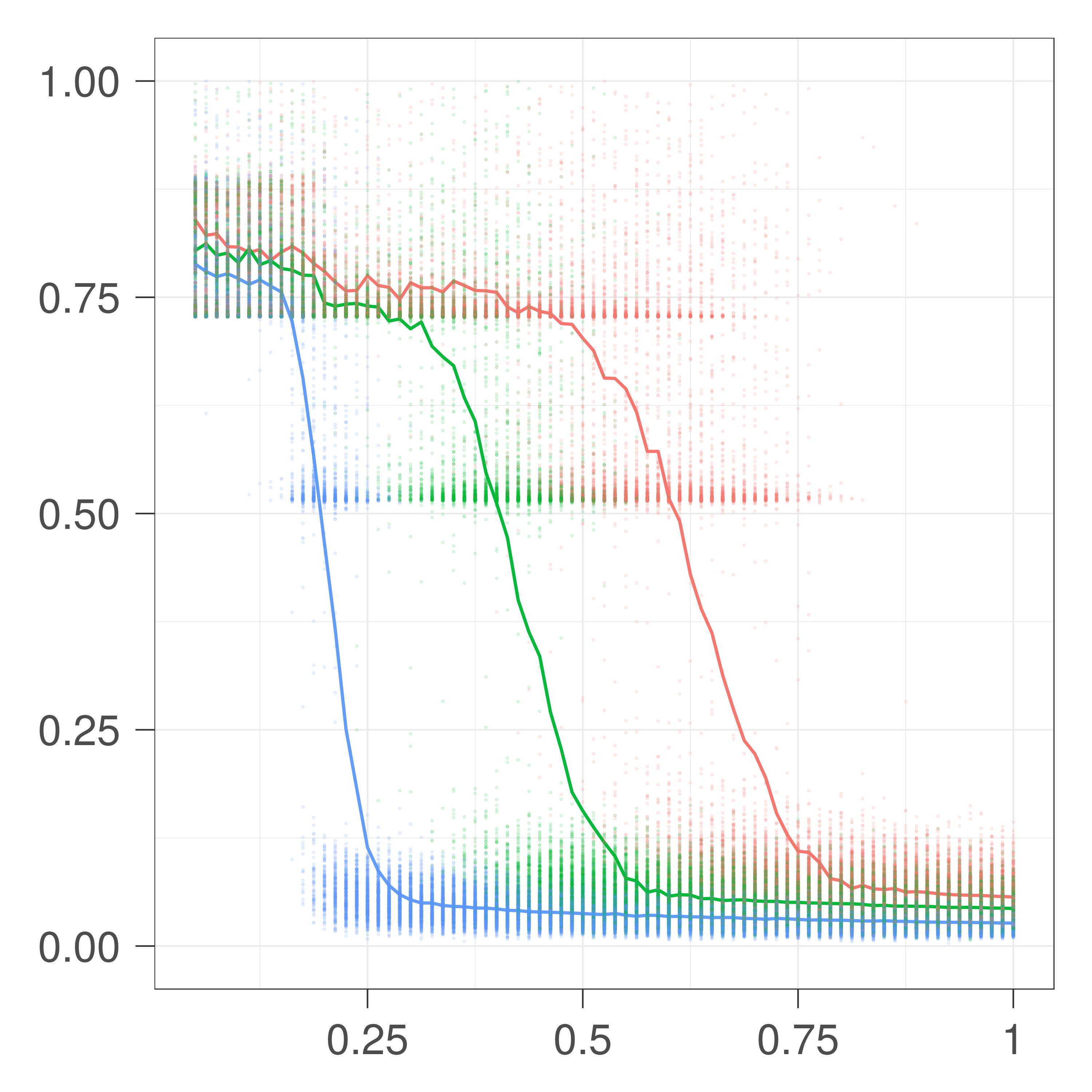
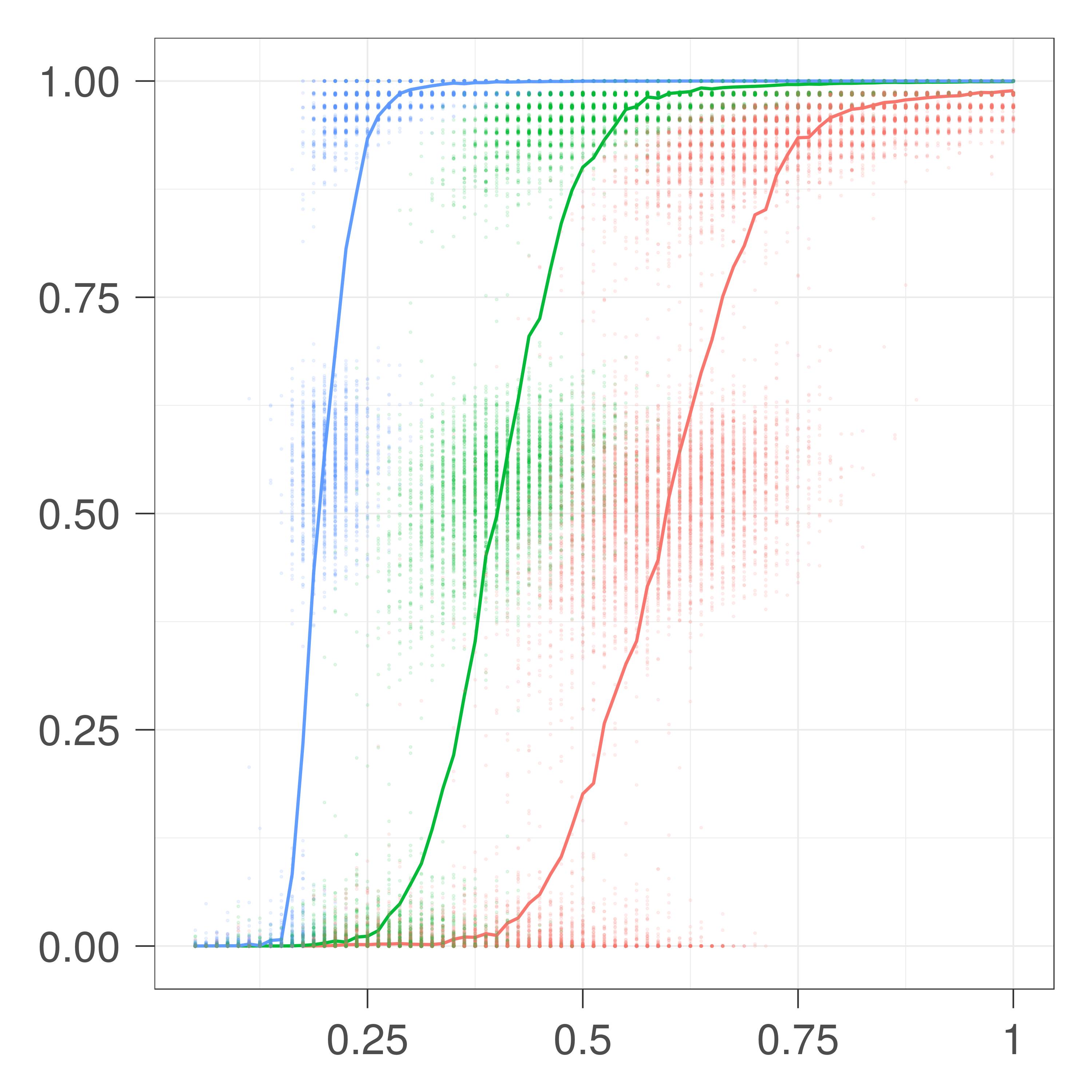
proportion of observed dyads

Figure 2: Estimation error of $\pi$ and Adjusted Rand Index averaged over 500 simulations in the MAR setting. The adjacency matrix $Y$ is generated under random-dyad sampling strategy for various connectivity $c=\sum_{q\ell}\alpha_{q}\alpha_{\ell}\pi_{q\ell}$.

4.2 NMAR condition

Under NMAR conditions we conduct an extensive simulation study by considering various network topologies (namely affiliation, star and bipartite), the connectivity matrix of which are given in Figure 3. We use a common tuning parameter $\epsilon$ to control the connectivity of the networks in each topology: the lower the $\epsilon$, the more contrasted the topology.

$\begin{pmatrix}1-\epsilon&\epsilon&\epsilon\\ \epsilon&1-\epsilon&\epsilon\\ \epsilon&\epsilon&1-\epsilon\\ \end{pmatrix}$

(a) affiliation

$\begin{pmatrix}1-\epsilon&1-\epsilon&0&0\\ 1-\epsilon&0&\epsilon&0\\ 0&\epsilon&1-\epsilon&1-\epsilon\\ 0&0&1-\epsilon&0\\ \end{pmatrix}$

(b) star

$\begin{pmatrix}\epsilon&1-\epsilon&\epsilon&\epsilon\\ 1-\epsilon&\epsilon&\epsilon&\epsilon\\ \epsilon&\epsilon&\epsilon&1-\epsilon\\ \epsilon&\epsilon&1-\epsilon&\epsilon\\ \end{pmatrix}$

(c) bipartite

Figure 3: Matrix $\pi$ in different topologies with inter/intra block probabilities.

Among the three schemes developed in Section 2.3.2, we investigate thoroughly the double standard sampling, for which we exhibit a large panel of situations where the gap is large between the performances of the algorithms designed for MAR or NMAR cases. Other sampling designs are explored in the supplementary materials.

Simulated networks have $n=100$ nodes, with $\epsilon$ varying in $\{0.05,0.15,0.25\}$. Prior probabilities $\alpha$ are chosen specifically for affiliation, star and bipartite topologies, respectively $(1/3,1/3,1/3)$, $(1/6,1/3,1/6,1/3)$ and $(1/4,1/4,1/4,1/4)$. The exploration of the sampling parameters $\psi=(\rho_{0},\rho_{1})$ is done on a grid $[0.1,0.9]\times[0.1,0.9]$ discretized by steps of $0.1$. Algorithm 2 is initialized with several random initializations and spectral clustering.

In Figure 4, the estimation error is represented as a function of the difference between the sampling design parameters $(\rho_{0},\rho_{1})$: the closer this difference to zero, the closer to the MAR case. As expected, Algorithm 1 designed for MAR only performs well when $\rho_{1}-\rho_{0}\approx 0$. Algorithm 2 designed for NMAR double-standard sampling shows relatively flat curves which means that its performances are roughly constant no matter the sampling condition.

	$\|\hat{\pi}-\pi\|_{F}/\|\pi\|_{F}$	ARI$(Z,\hat{Z})$
affiliation
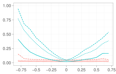
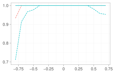
bipartite
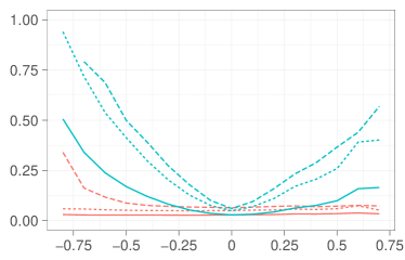
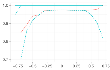
star
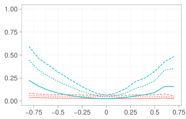
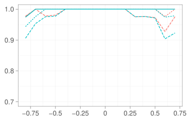
	$\rho_{1}-\rho_{0}$

Figure 4: Double standard setting: estimation error of $\pi$ and adjusted Rand index averaged over 500 simulations for affiliation, bipartite and star topologies.

$|\hat{\rho}_{0}-\rho_{0}|/|\rho_{0}|$	$|\hat{\rho}_{1}-\rho_{1}|/|\rho_{1}|$
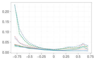
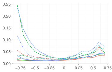
$\rho_{1}-\rho_{0}$

Figure 5: Double standard setting: estimation error of $\rho_{0}$ and $\rho_{1}$ averaged over 500 simulations for affiliation, bipartite and star topologies.

Figure 5 reports estimation accuracy for the sampling parameters $\rho_{0}$ and $\rho_{1}$. Results show a good ability of the VEM to estimate these parameters. As expected, performances deteriorate for uncontrasted topologies with low sampling rate.

Model selection.

Simulations are also conducted to study the performances of ICL. We compare results for the different topologies described in Figure 3 for $\epsilon=0.05$. Rates of correct answers for selecting the number of blocks $Q$ under a double standard sampling with different sampling rates are displayed in Table 1. The ARI is also provided. The ICL shows a satisfactory ability to select the true $Q$ even if the selection task obviously needs a larger sampling effort than the estimation task. It is worth mentioning that a whole block may not be sampled, which leads the ICL to select a lower number of blocks. In such a case the ARI is a meaningful additional information to demonstrate that the clustering remains coherent with the true one.

sampling rate	affiliation	bipartite	star
(0.154, 0.405]	0.58/0.96	0.46/0.84	0.45/0.84
(0.405, 0.656]	0.95/0.99	0.87/0.98	0.90/0.98
(0.656, 0.908]	1/1	0.99/1	0.99/1

Table 1: Performance of the ICL criterion: rates of correct answers when choosing the number of blocks and Adjusted Rand Indexes. Tested configurations are different sampling rates and three topologies (affiliation, bipartite and star) under a double standard sampling. Each configuration is simulated 500 times.

In Table 2, results concern the rates of correct selections of the sampling design when the two designs in competition are the random-dyad and the double standard samplings. As expected, the rate of correct answers increases with the sampling rate.

sampling rate	sampling	affiliation	bipartite	star
(0.096, 0.367]	MAR	0.73	0.67	0.63
	NMAR	0.72	0.75	0.75
(0.367, 0.638]	MAR	1	1	1
	NMAR	0.91	0.78	0.82
(0.638, 0.909]	MAR	1	1	1
	NMAR	0.91	0.8	0.95

Table 2: Rates of correct answers of the ICL criterion when choosing between Random-dyad sampling (MAR) and double standard sampling (NMAR) in each of the 18 configurations. A configuration is the combination of a topology (affiliation, bipartite and star), a sampling rate and a sampling design. Each configuration is simulated 500 times.

5 Importance of accouting for missing values in real networks

5.1 Seed exchange network in the region of Mount Kenya

In a context of subsistence farming, studies which investigate the relationships between crop genetic diversity and human cultural diversity patterns have shown that seed exchanges are embedded in farmers’ social organization. Data on seed exchanges of sorghum in the region of Mount Kenya were collected and analyzed in Labeyrie et al. (2016, 2014). The sampling is node-centered since the exchanges are documented by interviewing farmers who are asked to declare to whom they gave seeds and from whom they receive seeds. Since an interview is time consuming, the sampling is not exhaustive. A limited space area was defined where all the farmers were interviewed. The network is thus collected with missing dyads since information on the potential links between two farmers who were cited but not interviewed is missing. With the courtesy of Vanesse Labeyrie, we analyzed the Mount Kenya seed exchange network involving $568$ farmers among which $155$ were interviewed. Although other farmers in this region might be connected to non-interviewed farmers, we focus on this closed network of $568$ nodes.

Since we only know that the sampling is node-centered, we fit SBM under the three node-centered sampling designs presented in Section 2.2 (star (MAR), class and star degree sampling). The ICL criterion is minimal for $10$ blocks under the star degree sampling and for $11$ blocks under the class degree sampling. The clusterings between the SBMs obtained with either class or star degree sampling remain close from each other (ARI: $0.6$) and both unravel a strong community structure. The model selected by ICL for MAR sampling is composed by $11$ blocks. The ARIs between MAR clustering and the two other clusterings are lower (around $0.4$). Finally, note that interviewed and non-interviewed farmers are mixed up in the blocks of the three selected models. The ICL criteria computed for the three sampling designs are a slightly in favor of the MAR sampling.

On top of network data, categorical variables are available for discriminating the farmers such as the ntora they belong to ($10$ main ntoras plus $1$ grouping all the others) and the dialect they speak ($4$ dialects). In Figure 6, we compute ARIs between the ntoras (left panel), the dialects (right panel) and the clusterings obtained with the SBM under the three node-centered sampling designs for a varying number of blocks. Even though the ARIs remain low, the clusterings from class or star degree sampling seem to catch a non negligible fraction of the social organization, larger than the one caught by the clustering from the MAR sampling. These two categorical variables, reflecting some aspects of the social organization, could partially explain the structure of the exchange network.

ARI
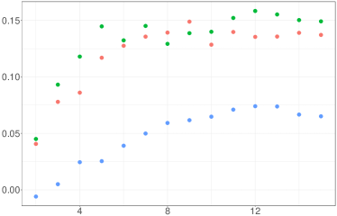
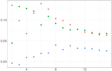
number of blocks

Figure 6: ARIs computed between the clusterings given by an SBM under class, star degree and MAR samplings with a varying number of blocks $Q$ and ntora of farmers (left-hand-side) or dialect spoken by farmers (right-hand-side)

5.2 ER (ESR1) Protein-Protein Interaction network in breast cancer

Estrogen receptor 1 (ESR1) is a gene that encodes an estrogen receptor protein (ER), a central actor in breast cancer. Uncovering its relations with other proteins is essential for a better understanding of the disease. To this end, various bioinformatics tools are available to centralize knowledge about possible relations between proteins into networks known as Protein-Protein Interaction (PPI) networks. The platform string (Szklarczyk et al., 2015) accessible via http://www.string-db.org is one of the most popular tools for this task. Given a set of one (or several) initial protein(s) provided by the user, it is possible to recover a valued network between all proteins connected to the initial set. The value of an edge in this network corresponds to a score obtained by aggregating different types of knowledge (wet-lab experiments, textmining, co-expression data, etc…), reflecting a level of confidence. Thus, it is possible for a given protein – we choose ER here – to recover the PPI network between all proteins involved. Our ambition is to rely on a SBM with missing data to finely analyze such networks: we rather describe a dyad as missing (thus not choosing between 0 or 1) if its level of confidence is too low.

The PPI network in the neighborhood of ER is composed by 741 proteins connected by edges with values in $(0,1]$. We remove ER from this set of proteins, as well as the zinc finger protein 44. Indeed, they were both connected to most of the other proteins and would thus only blur the underlying clustering structure. We denote $\omega_{ij}$ the weight associated with dyad $(i,j)$. By means of a tuning parameter $\gamma$ reflecting the level of confidence, the adjacency matrix is defined as follows:

$$\mathbf{A}^{\gamma}=\left(A^{\gamma}\right)_{ij}=\left\{\begin{array}[]{ll}1&\text{if }\omega_{ij}>1-\gamma,\\ \texttt{NA}&\text{if }\gamma\leq\omega_{ij}\leq 1-\gamma,\\ 0&\text{if }\omega_{ij}<\gamma.\\ \end{array}\right.$$ (15)

In order to analyze the ER-centered network, Algorithm 1 (random-dyad MAR sampling) and Algorithm 2 (double-standard NMAR sampling) were applied on $\mathbf{A}^{\gamma}$ for $\gamma$ varying in $\{.15,.25,.35\}$, hence taking the uncertainties on the missing dyads into account with various thresholds. The ICL criterion in Figure 7 systematically chooses the NMAR modeling against the MAR modeling, whatever the value of $\gamma$.

	$\gamma=.15$	$\gamma=.25$	$\gamma=.35$
ICL
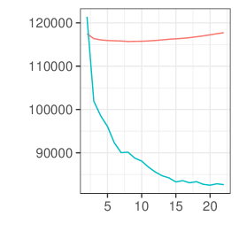
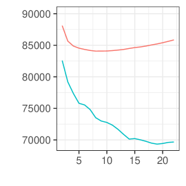
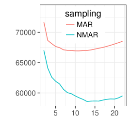
		number of blocks

Figure 7: ICL criteria for SBMs with random-dyad MAR sampling and double-standard NMAR sampling in the thresholded ER network.

We study the best MAR and NMAR models associated with $\gamma=0.35$, which value exhibits a clearer choice of the ICL than for $\gamma=\{.15,.25\}$ for both MAR and NMAR modelings. The two corresponding SBMs have 11 clusters for MAR sampling and 13 clusters for NMAR sampling. The ARI between the two clusterings is around $0.39$: this is mainly due to a large block in the random-dyad MAR clustering which contains much more nodes than any of the blocks in the NMAR clustering. The latter dispatches many of these nodes in four blocks (see the supplementary materials for a more detailed exposition of results). To prove that this finest clustering of the nodes is more relevant from the biological point of view, we propose a validation based on external biological knowledge. To this end, we rely on the Gene Ontology (GO) annotation (Ashburner et al., 2000) which provides a DAG of ontologies to which genes are annotated if the proteins encoded by these genes are involved in a known biological process. Here, we use GO to perform enrichment analysis (that is to say identifying classes of genes that are over-represented in a large set of genes, via a simple hypergeometric test) on genes corresponding to the proteins present in the large block for MAR, and the corresponding four blocks for NMAR. Interestingly, at a significance level of $1\%$, we find a single significant biological process for MAR modeling while 13 are found significant in the NMAR case. We check that it is not due to a simple threshold effect by looking at the ranks of the $p$-values of the 13 NMAR significant processes in the 100 first most significant terms found in the MAR model: only 5 of the NMAR processes are found, with high ranks (24, 33, 39, 56 and 77) far from the smallest MAR $p$-values.

6 Conclusion

This paper shows how to deal with missing data on dyads in the SBM. We study MAR and NMAR sampling designs motivated by network data and propose variational approaches to perform inference under this series of designs, accompanied with model selection criteria. Relevance of the method is illustrated on numerical experiments both on simulated and real-world networks. An R-package is available at https://github.com/jchiquet/missSBM. .

This work focuses on undirected binary networks. However, it can be adapted to other SBMs, in particular those developed in Mariadassou et al. (2010) for (un)directed valued networks with a distribution of weights belonging to the exponential family. It could also be adapted to the degree-corrected SBM (Karrer and Newman, 2011), where the sampling design would depend on the degree correction parameters. This should lead to a design close to the star degree sampling. In future works, we plan to investigate the consistency of the variational estimators of SBM under missing data conditions, looking for similar results as the ones obtained in Bickel et al. (2013) for fully observed networks. Another path of research is to consider missing data where we cannot distinguish between a missing dyad and the absence of an edge like in Priebe et al. (2015), Balachandran et al. (2017).

Acknowledgment.

The authors thank Sophie Donnet (INRA-MIA, AgroParisTech) and Mahendra Mariadassou (INRA-MaIAGE, Jouy-en-Josas) for their helpful remarks and suggestions. We also thank all members of MIRES for fruitful discussions on network sampling designs and for providing the original problems from social science. In particular, we thank Vanesse Labeyrie (CIRAD-Green) for sharing the seed exchange data and for related discussions on the analysis.

This work is supported by the INRA MetaProgram « GloFoods » through the project « SEARS » and by two public grants overseen by the French National research Agency (ANR): first as part of the « Investissement d’Avenir » program, through the « IDI 2017 » project funded by the IDEX Paris-Saclay, ANR-11-IDEX-0003-02, and second by the « EcoNet » project.

References

- Aicher et al. (2014) C. Aicher, A. Z. Jacobs, and A. Clauset. Learning latent block structure in weighted networks. J. Compl. Net., 3.2:221–248, 2014.
- Airoldi et al. (2008) E. M. Airoldi, D. M. Blei, S. E. Fienberg, and E. P. Xing. Mixed membership stochastic blockmodels. J. Mach. Learn. Res., 9(Sep):1981–2014, 2008.
- Ashburner et al. (2000) M. Ashburner, C. A. Ball, J. A. Blake, D. Botstein, H. Butler, J. M. Cherry, A. P. Davis, K. Dolinski, S. S. Dwight, J. T. Eppig, et al. Gene ontology: tool for the unification of biology. Nat. Genet., 25(1):25, 2000.
- Balachandran et al. (2017) P. Balachandran, E. D. Kolaczyk, and W. D. Viles. On the propagation of low-rate measurement error to subgraph counts in large networks. Journal of Machine Learning Research, 18(61):1–33, 2017.
- Barbillon et al. (2015) P. Barbillon, S. Donnet, E. Lazega, and A. Bar-Hen. Stochastic block models for multiplex networks: an application to networks of researchers. J. R. Stat. Soc. C-Appl., 2015.
- Bickel et al. (2013) P. Bickel, D. Choi, X. Chang, H. Zhang, et al. Asymptotic normality of maximum likelihood and its variational approximation for stochastic blockmodels. Ann. Stat., 41(4):1922–1943, 2013.
- Biernacki et al. (2000) C. Biernacki, G. Celeux, and G. Govaert. Assessing a mixture model for clustering with the integrated completed likelihood. IEEE Trans. Pattern Anal. Mach. Intell., 22(7):719–725, 2000.
- Celisse et al. (2012) A. Celisse, J.-J. Daudin, L. Pierre, et al. Consistency of maximum-likelihood and variational estimators in the stochastic block model. Electron. J. Stat., 6:1847–1899, 2012.
- Chatterjee (2015) S. Chatterjee. Matrix estimation by universal singular value thresholding. The Annals of Statistics, 43(1):177–214, 2015.
- Daudin et al. (2008) J.-J. Daudin, F. Picard, and S. Robin. A mixture model for random graphs. Stat. comp., 18(2):173–183, 2008.
- Davenport et al. (2014) M. A. Davenport, Y. Plan, E. van den Berg, and M. Wootters. 1-bit matrix completion. Information and Inference: A Journal of the IMA, 3(3):189–223, 2014.
- Frank and Harary (1982) O. Frank and F. Harary. Cluster inference by using transitivity indices in empirical graphs. J. Am. Stat. Soc., 77(380):835–840, 1982.
- Goldenberg et al. (2010) A. Goldenberg, A. X. Zheng, S. E. Fienberg, E. M. Airoldi, et al. A survey of statistical network models. Foundations and Trends® in Machine Learning, 2(2):129–233, 2010.
- Handcock and Gile (2010) M. S. Handcock and K. J. Gile. Modeling social networks from sampled data. The Annals of Applied Statistics, 4(1):5–25, 2010.
- Holland et al. (1983) P. W. Holland, K. B. Laskey, and S. Leinhardt. Stochastic blockmodels: First steps. Social networks, 5(2):109–137, 1983.
- Jordan et al. (1998) M. I. Jordan, Z. Ghahramani, T. S. Jaakkola, and L. K. Saul. An introduction to variational methods for graphical models. In Learning in graphical models, pages 105–161. Springer, 1998.
- Karrer and Newman (2011) B. Karrer and M. E. J. Newman. Stochastic blockmodels and community structure in networks. Phys. Rev. E, 83:016107, Jan 2011.
- Kolaczyk (2009) E. D. Kolaczyk. Statistical analysis of network data, methods and models. Springer, 2009.
- Labeyrie et al. (2014) V. Labeyrie, M. Deu, A. Barnaud, C. Calatayud, M. Buiron, P. Wambugu, S. Manel, J.-C. Glaszmann, and C. Leclerc. Influence of ethnolinguistic diversity on the sorghum genetic patterns in subsistence farming systems in eastern kenya. PLoS One, 9(3):e92178, 2014.
- Labeyrie et al. (2016) V. Labeyrie, M. Thomas, Z. K. Muthamia, and C. Leclerc. Seed exchange networks, ethnicity, and sorghum diversity. P. Natl. Acad. Sci., 113(1):98–103, 2016.
- Latouche et al. (2011) P. Latouche, É. Birmelé, and C. Ambroise. Overlapping stochastic block models with application to the french political blogosphere. Ann. Appl. Stat., pages 309–336, 2011.
- Latouche et al. (2012) P. Latouche, É. Birmelé, and C. Ambroise. Variational bayesian inference and complexity control for stochastic block models. Stat. Modelling, 12(1):93–115, 2012.
- Latouche et al. (2017) P. Latouche, S. Robin, and S. Ouadah. Goodness of fit of logistic models for random graphs. Technical report, 2017. URL https://arxiv.org/abs/1508.00286.
- Little and Rubin (2014) R. J. Little and D. B. Rubin. Statistical analysis with missing data. John Wiley & Sons, 2014.
- Mariadassou et al. (2010) M. Mariadassou, S. Robin, and C. Vacher. Uncovering latent structure in valued graphs: A variational approach. Ann. Appl. Stat., 4(2):715–742, 06 2010.
- Matias and Miele (2016) C. Matias and V. Miele. Statistical clustering of temporal networks through a dynamic stochastic block model. J. R. Stat. Soc. B-Met., 2016.
- Matias and Robin (2014) C. Matias and S. Robin. Modeling heterogeneity in random graphs through latent space models: a selective review. ESAIM Proc. Sur., 47:55–74, 2014.
- Molenberghs et al. (2008) G. Molenberghs, C. Beunckens, C. Sotto, and G. M. Kenward. Every missing not at random model has got a missing at random counterpart with equal fit. J. R. Stat. Soc. B-Met., 2008.
- Nowicki and Snijders (2001) K. Nowicki and T. A. B. Snijders. Estimation and prediction for stochastic blockstructures. J. Am. Stat. Soc., 96(455):1077–1087, September 2001.
- Priebe et al. (2015) C. E. Priebe, D. L. Sussman, M. Tang, and J. T. Vogelstein. Statistical inference on errorfully observed graphs. Journal of Computational and Graphical Statistics, 24(4):930–953, 2015.
- Rand (1971) W. M. Rand. Objective criteria for the evaluation of clustering methods. J. Am. Stat. Soc., 66(336):846–850, 1971.
- Rubin (1976) D. B. Rubin. Inference and missing data. Biometrika, 63(3):581–592, 1976.
- Snijders (2011) T. A. Snijders. Statistical models for social networks. Annual Review of Sociology, 37:131–153, 2011.
- Snijders and Nowicki (1997) T. A. Snijders and K. Nowicki. Estimation and prediction for stochastic blockmodels for graphs with latent block structure. J. class., 14(1):75–100, 1997.
- Szklarczyk et al. (2015) D. Szklarczyk, A. Franceschini, S. Wyder, K. Forslund, D. Heller, J. Huerta-Cepas, M. Simonovic, A. Roth, A. Santos, K. P. Tsafou, et al. String v10: protein–protein interaction networks, integrated over the tree of life. Nucleic. Acids Res., 43, 2015.
- Thompson and Frank (2000) S. K. Thompson and O. Frank. Model-based estimation with link-tracing sampling designs. Survey Methodology, 26(1):87–98, 2000.
- Thompson and Seber (1996) S. K. Thompson and G. Seber. Adaptive Sampling. New-York : Wiley, 1996.
- Vinayak et al. (2014) R. K. Vinayak, S. Oymak, and B. Hassibi. Graph clustering with missing data: Convex algorithms and analysis. Adv. Neu. In., 2014.
- Vincent and Thompson (2015) K. Vincent and S. Thompson. Estimating the size and distribution of networked populations with snowball sampling. Technical report, 2015. URL http://arxiv.org/abs/1402.4372v2.