Material Optimization in Transverse Electromagnetic Scattering Applications

Abstract

A class of algorithms for the solution of discrete material optimization problems in electromagnetic applications is discussed. The idea behind the algorithm is similar to that of the sequential programming. However, in each major iteration a model is established on the basis of an appropriately parametrized material tensor. The resulting nonlinear parametrization is treated on the level of the sub-problem, for which, globally optimal solutions can be computed due to the block separability of the model. Although global optimization of non-convex design problems is generally prohibitive, a well chosen combination of analytic solutions along with standard global optimization techniques leads to a very efficient algorithm for most relevant material parametrizations. A global convergence result for the overall algorithm is established. The effectiveness of the approach in terms of both computation time and solution quality is demonstrated by numerical examples, including the optimal design of cloaking layers for a nano-particle and the identification of multiple materials with different optical properties in a matrix.

35Q60, 35R30, 90C26, 90C35, 90C90

1 Introduction

Problems of material optimization governed by Maxwell’s equation have recently been studied in the literature. In particular, for time-harmonic electromagnetic fields we refer to [5], where an optimal distribution of two materials with distinct properties was computed based on the so-called SIMP approach [1]. This approach was originally developed for the topology optimization of elastic structures and is based on interpolation between the desired material properties and an appropriate penalization scheme rendering undesired intermediate material properties unattractive with respect to the particular cost function. A similar technique has been applied to the transient problem discussed, for example in [10]. Again the goal here was to find an optimal distribution of two isotropic materials. Potential applications of structural optimization techniques in the context of electromagnetics range from inverse problems, where distribution of material is reconstructed by the information given by the scattered electromagnetic fields [13], to optimal material layout to improve the properties of optical devices [3] or nanoparticles [18].

In this paper we are interested in a more general class of material optimization problems, in the framework of which a complex-valued permittivity tensor for a given point in the design domain is specified by a function of a finite number of parameters. Particular realizations have led to problems of free material optimization [28, 8, 1, 19], which have so far been studied solely in the context of linear elasticity, to optimal material orientation problems, see e.g. [17], and to so called discrete multi-material optimization as treated in literature by so called DMO methods, see, e.g. [23, 11]. Rather than formulating the optimization problems directly in the design parameters and using a derivative based optimization algorithm like SNOPT [7] or MMA [25] in a “black box” way, in this article, a new algorithmic concept for the solution of the envisaged class of design problems is developed. The motivation for the development of this new solution approach is the fact that the material tensors typically depend on the design parameters in a non-linear way and thus the parametrization may result in numerous poor local optima, see [17], in which algorithms applied in a black-box way may become trapped.

In order to prevent this, the following concept is suggested: the principal idea is to formulate the design problem directly in terms of the material tensors, while the associated parametrization is hidden in the definition of the admissible set. Then, in the course of a sequential approximation algorithm, FMO-type models (see [24]) of the objective as a function of the material tensors are derived and are used to generate a sequence of sub-problems. Due to the potentially non-convex parametrization each sub-problem is a constrained non-linear optimization problem, which may exhibit an unknown number of local optima. We show that based on the properties of the particular approximations these sub-problems can be solved to global optimality with a reasonable effort, partially with the analytical solution, for important classes of parametrizations.

The manuscript is structured as follows: In Section 2 the Helmholtz-type state equation, based on the time-harmonic Maxwells equation, is given in its weak formulation and the dependency on the material tensor is highlighted. Then, in Section 3 the class of optimization problems of interest is stated, including a detailed description of the general structure of the objective function as well as the structure of the set of admissible materials, which is based on a graph. The discussion is continued with a short note on the discretization of the state and the optimization problem as well as regularization issues. Section 4 constitutes the heart of this article. Based on convex first-order hyperbolic approximation as well as a so-called sequential global programming technique, an optimization algorithm is stated for which a global convergence result can be established. Subsequently, parametrization-dependent solutions to the sub-problems taking the graph-structure of the admissible set into account are derived. To show the capabilities of the algorithm, two examples are discussed in Section 5. These include both the design of a cloaking for a scatterer made from an increasing number of anisotropic materials and the tomographic reconstruction of an unknown material distribution consisting of a background material, a dielectric and an absorbing material.

Throughout this paper, we indicate by $\mathbb{S}_{\mathds{C}}$ the space of symmetric, two-dimensional and complex-valued tensors. The term $\langle A,B\rangle:=\operatorname{Re}(\operatorname{tr}(A^{H}B))$ denotes the standard scalar product in $\mathbb{S}_{\mathds{C}}$ and $\|A\|^{2}_{F}=\langle A,A\rangle$ denotes the induced Frobenius norm.

For a real-valued continuously differentiable function $v:\mathbb{S}_{\mathds{C}}\to\mathds{R}$ we define the derivative of $v$ in a direction $Y\in\mathbb{S}_{\mathds{C}}$ with respect to $B$ as

$$\frac{\partial v(B)}{\partial B}[Y]:=\lim_{\nu\to 0}\frac{v(B+\tau Y)-v(B)}{\nu}.$$

We note that for the tuple ${\boldsymbol{B}}\in\mathbb{S}^{{K}}_{\mathds{C}}$ with ${K}\in\mathds{N}$ and a real-valued continuously differentiable function $v:\mathbb{S}^{{K}}_{\mathds{C}}\to\mathds{R}$, the directional derivative of $v$ in direction $\boldsymbol{Y}\in\mathbb{S}^{{K}}_{\mathds{C}}$ with respect to ${\boldsymbol{B}}$ is given as

$$\frac{\partial v({\boldsymbol{B}})}{\partial{\boldsymbol{B}}}[\boldsymbol{Y}]=\sum_{i=1}^{K}\frac{\partial v({\boldsymbol{B}})}{\partial({\boldsymbol{B}})_{i}}[(\boldsymbol{Y})_{i}].$$

Finally, we define the extended norm $\|{\boldsymbol{B}}\|^{2}_{F^{K}}:=\sum_{i=1}^{K}\|({\boldsymbol{B}})_{i}\|^{2}_{F}$ for ${\boldsymbol{B}}\in\mathbb{S}^{{K}}_{\mathds{C}}$.

2 Prerequisites

The propagation of electromagnetic waves is described by Maxwell’s equation [12]. In this paper we restrict ourselves to the time-harmonic propagation of so-called transverse magnetic waves (TM) for a given wavenumber $\omega$, where we assume that the electromagnetic field is given by a scalar function depending only on two spatial dimensions. With these assumptions, Maxwell’s equation simplifies to the Helmholtz equation for the magnetic field.

The relative permittivity $\varepsilon$, which in this article is the material property of interest, is a complex- and tensor-valued function of space. For modeling purposes an additional tensor valued function $B$ is introduced, whose values are given by the inverse of the permittivity at each point. In general, we assume that the material tensor at a point is symmetric, i. e. $B:\mathds{R}^{2}\to\mathbb{S}_{\mathds{C}}$. For scattering applications an incident magnetic field $u_{I}:\mathds{R}^{2}\to\mathds{C}$ is given, which solves Maxwell’s equation for the given background material $B_{b}:\mathds{R}^{2}\to\mathbb{S}_{\mathds{C}}$. The Helmholtz equation is actually defined on the whole of $\mathds{R}^{2}$, thus we introduce a perfectly matched layer (PML) [2] surrounding the domain of interest, including the scattering object.

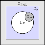
Figure 1: General geometrical setting: PML, background and design domain

The computational domain $\Omega=\Omega_{D}\cup\Omega_{C}\subset\mathds{R}^{2}$ is subdivided into a design domain $\Omega_{D}$ and a non-design domain $\Omega_{C}$. The non-design domain $\Omega_{C}=\Omega_{\text{PML}}\cup\Omega_{b}\cup\Omega_{P}$ in turn consists of three subdomains. The perfectly matched layer $\Omega_{\text{PML}}$ completely encloses the background domain $\Omega_{b}$ and both are equipped with background material tensor-valued function $B_{b}$. Moreover, the scatterer domain $\Omega_{P}$ and the design domain $\Omega_{D}$ are both embedded in the background domain $\Omega_{b}$ (see Fig. 1). The tensor valued function $B_{P}:\Omega_{P}\to\mathbb{S}_{\mathds{C}}$ in the scatterer domain is assumed to be independent of the design, whereas the tensor function $B:\Omega_{D}\to\mathbb{S}_{\mathds{C}}$ associated with the design domain $\Omega_{D}$ will be subject to optimization. For the sake of notation, we combine both functions to the piecewise tensor-valued function $B_{C}:\Omega_{C}\to\mathbb{S}_{\mathds{C}}$ with

$$B_{C} =\begin{cases}B_{b}&\text{ in }\Omega_{b}\cup\Omega_{\text{PML}},\\ B_{P}&\text{ in }\Omega_{P}.\end{cases}$$

Using this, we state the Helmholtz equation in weak form:

$${\text{Find }u\in H^{1}_{0}(\Omega,\mathds{C})\ \operatorname{s.t.}} a(B;u,\varphi)+a_{C}(u,\varphi)=l(B;\varphi)+l_{C}(\varphi)\quad\text{ for all }\varphi\in H^{1}_{0}(\Omega).$$

Here, we explicitly point out the dependency on $B$ and note the subdivision of the bilinear and linear forms into design domain contributions

$$a(B;u,\varphi) =\int_{\Omega_{D}}B\nabla u\cdot\nabla\varphi-\omega^{2}u\varphi\,\mathrm{d}x, l(B;\varphi) =-\int_{\Omega_{D}}B\nabla u_{I}\cdot\nabla\varphi\,\mathrm{d}x$$

and non-design domain contributions

$$a_{C}(u,\varphi) =\int_{\Omega_{C}}B_{C}A^{\omega}_{\varepsilon}\nabla u\cdot\nabla\varphi-\omega^{2}A^{\omega}_{\mu}u\varphi\,\mathrm{d}x,$$

$$l_{C}(\varphi) =\int_{\Omega}B_{b}\nabla u_{I}\cdot\nabla\varphi\,\mathrm{d}x-\int_{\Omega_{C}}B_{C}\nabla u_{I}\cdot\nabla\varphi\,\mathrm{d}x.$$

By the definition of $B_{C}$ we observe that the right hand side of (2) vanishes in $\Omega_{b}\cup\Omega_{\text{PML}}$. The functions $A^{\omega}_{\varepsilon}$ and $A^{\omega}_{\mu}$ describe the wavelength dependent PML [16] based on a squared layer with distance $d$ from the origin and are defined as follows:

$$A^{\omega}_{\epsilon}(x,y) =\begin{pmatrix}\frac{s(y)}{s(x)}&0&\\ 0&\frac{s(x)}{s(y)}\end{pmatrix}, A^{\omega}_{\mu}(x,y) =s(x)s(y), s(t) =1-\frac{\sigma_{0}\max(0,|t|-d)}{\imath\omega}.$$

Particular choices of the positive scalar $\sigma_{0}$ and $d$ depend on the particular application, see Section 5. The definition of $s$ implies that $A^{\omega}_{\epsilon}\equiv\mathds{1}$ and $A^{\omega}_{\mu}\equiv 1$ in $\Omega\setminus\Omega_{\text{PML}}$.

3 A general material optimization problem

Figure 2: Example graph of admissible set $\mathcal{G}$

We start with the description of the set of admissible material tensors $\mathcal{G}$, which is structured by a graph $(V,E)$ with vertices $V$ and edges $E=\{e_{1},\dotsc,e_{N_{E}}\}\subset V\times V$. We assume that every vertex $v\in V$ is part of at least one edge and is associated with a predefined material tensor $B^{(v)}\in\mathbb{S}_{\mathds{C}}$, cf. Fig. 2. We further define $\mathcal{N}:=\{B^{(v)}\mid v\in V\}$, $\mathcal{I}_{E}:=\{1,\dotsc,{N_{E}}\}$ and introduce the following parametrization:

Definition 3.1 (parametrization of $\mathcal{G}$).

We call the mapping $\psi:\mathcal{I}_{E}\times[0,1]\to\mathbb{S}_{\mathds{C}}$ parametrization of $\mathcal{G}$ iff the following holds:

• $\psi$ is twice continuously differentiable with respect to the second variable.

• interpolation property:

  $$\psi(l,0)=B^{e_{l}^{(1)}}\text{ and }\psi(l,1)=B^{e_{l}^{(2)}}\quad\forall l\in\mathcal{I}_{E},$$

  where $e_{l}^{(1)}$ and $e_{l}^{(2)}$ denote the first and second node of the $l$-th edge, respectively.

• $\psi$ is injective on $\mathcal{I}_{E}\times(0,1)$, i. e.

  $$\forall(k,s),(l,t)\in\mathcal{I}_{E}\times(0,1):\psi(k,s)=\psi(l,t)\Rightarrow(k,s)=(l,t).$$

We denote the image generated by the parametrization on the $l$-th edge by $\mathcal{E}_{l}$, i. e.

$$\mathcal{E}_{l}=\{\psi(l,\delta)\mid\delta\in[0,1]\},\quad\forall l\in\mathcal{I}_{E}.$$

Thus the set of admissible material tensors can be written as

$$\mathcal{G}=\{\psi(l,\delta)\mid(l,\delta)\in\mathcal{I}_{E}\times[0,1]\}=\mathcal{E}_{1}\cup\dotsb\cup\mathcal{E}_{N_{E}}$$

and the set $\mathrm{G}$ of admissible tensor-valued material distribution reads as

$$\mathrm{G}=\{B:\Omega_{D}\to\mathbb{S}_{\mathds{C}}\mid B(x)\in\mathcal{G}\text{ for }x\in\Omega_{D}\}.$$

Particular choices of $\mathrm{G}$ are given in Section 5. In the following, we use the notation $\psi_{l}(\delta):=\psi(l,\delta)$ for all $l\in\mathcal{I}_{E},\delta\in[0,1]$. Using this, we state an optimal design problem of tensor-valued coefficients over a Helmholtz-type equation in the domain $\Omega$ as follows:

(1) $$\left\{\quad\begin{aligned} \min_{B\in\mathrm{G}}~{}&J^{p}(B,u)+\eta J^{r}(B)+\gamma J^{g}(B)\\ \operatorname{s.t.}~{}&u\in H^{1}_{0}(\Omega,\mathds{C})\text{ is the solution of }&\\ &\begin{multlined}a(B;u,\varphi)+a_{C}(u,\varphi)=l(B;\varphi)+l_{C}(\varphi)\quad\text{ for all }\varphi\in H^{1}_{0}(\Omega)\end{multlined}a(B;u,\varphi)+a_{C}(u,\varphi)=l(B;\varphi)+l_{C}(\varphi)\quad\text{ for all }\varphi\in H^{1}_{0}(\Omega)\end{aligned}\right.$$

The real-valued function $J^{p}$ is called the objective functional and is assumed to be Gateaux-differentiable on $\mathrm{G}\times H^{1}_{0}(\Omega,\mathds{C})$ with respect to both the complex- and tensor-valued material distribution $B$ and the state variable $u$.

Moreover, $J^{r}$ and $J^{g}$ are Gateaux-diffentiable functionals that penalize irregular and undesired material distributions $B$, respectively, and $\eta$ and $\gamma$ are non-negative scalars. We refer to Sections 3.2 and 4.3 for precise definitions.

3.1 Discretization

Let $\boldsymbol{T}$ be a regular triangulation of $\Omega$ with ${N_{T}}$ triangular elements $T_{i}$, $1\leq i\leq{N_{T}}$, where the first ${K}$ triangles are located in the design domain $\Omega_{D}$. We assume that all subdomains in $\Omega$ are exactly approximated by the triangulation.

The tensor-valued function $B$ is assumed to be constant on each triangle $T_{i}$, $i\in\mathcal{I}_{D}:=\{1,\dotsc,{K}\}$ of the design domain, i. e. $B(x)|_{\Omega_{D}}=B_{h}(x):=\sum_{i=1}^{K}({\boldsymbol{B}})_{i}\chi_{T_{i}}(x)$ with a tuple ${\boldsymbol{B}}\in\mathbb{S}^{{K}}_{\mathds{C}}$ and the characteristic function $\chi_{T_{i}}$ of triangle $T_{i}$. Furthermore, the state $u:\Omega\to\mathds{C}$ is approximated by $u_{h}(x):=\sum_{i=1}^{N_{p}}({\boldsymbol{u}})_{i}\varphi_{i}(x)$ with ${N_{p}}$ degrees of freedom entering the coefficient vector ${\boldsymbol{u}}\in\mathds{C}^{N_{p}}$. In summary, the optimization problem (1) is approximated by

(2) $$\left.\begin{aligned} \min_{{\boldsymbol{B}}\in\mathcal{B}}~{}&J^{p}_{h}({\boldsymbol{B}},{\boldsymbol{u}})+\eta J^{r}_{h}({\boldsymbol{B}})+\gamma J^{g}_{h}({\boldsymbol{B}})\\ \operatorname{s.t.}~{}&(S({\boldsymbol{B}})+S_{C}){\boldsymbol{u}}=(H({\boldsymbol{B}})+H_{C})\end{aligned}\qquad\right.$$

with the admissible set $\mathcal{B}:=(\mathcal{G})^{K}$ and discretized versions of the objective functional $J^{p}_{h}({\boldsymbol{B}},{\boldsymbol{u}}):=J^{p}(B_{h},u_{h})$, regularization functional $J^{r}_{h}({\boldsymbol{B}}):=J^{r}(B_{h})$ and penalization functional $J^{g}_{h}({\boldsymbol{B}}):=J^{g}(B_{h})$. The PDE constraint is approximated by a system of equations with the symmetric matrices $S({\boldsymbol{B}}),S_{C}\in\mathds{C}^{{N_{p}}\times{N_{p}}}$, which are defined entry-wise by

$$(S({\boldsymbol{B}}))_{ij} =\sum_{k=1}^{K}\int_{T_{k}}B_{k}\nabla\varphi_{i}\cdot\nabla\varphi_{j}-\omega^{2}\varphi_{i}\varphi_{j}\,\mathrm{d}x, \text{for all }1\leq i,j\leq{N_{p}}$$

$$(S_{C})_{ij} =\int_{\Omega_{C}}B_{C}A^{\omega}_{\epsilon}\nabla\varphi_{i}\cdot\nabla\varphi_{j}-\omega^{2}A^{\omega}_{\mu}\varphi_{i}\varphi_{j}\,\mathrm{d}x \text{for all }1\leq i,j\leq{N_{p}}.$$

Finally, the right hand side vectors $H({\boldsymbol{B}}),H_{C}\in\mathds{C}^{N_{p}}$ are defined by

$$(H({\boldsymbol{B}}))_{i} =\sum_{k=1}^{K}\int_{T_{k}}B_{k}\nabla u_{I}\cdot\nabla\varphi_{i}\,\mathrm{d}x \text{for all }1\leq i\leq{N_{p}}$$

$$(H_{C})_{i} =\int_{\Omega_{C}}B_{C}\nabla u_{I}\cdot\nabla\varphi_{i}\,\mathrm{d}x-\int_{\Omega}B_{b}\nabla u_{I}\cdot\nabla\varphi_{i}\,\mathrm{d}x \text{for all }1\leq i,j\leq{N_{p}}.$$

We note that the solution ${\boldsymbol{u}}$ of the discretized state problem

(3) $$(S({\boldsymbol{B}})+S_{C}){\boldsymbol{u}}=H({\boldsymbol{B}})+H_{C}$$

is uniquely defined by the material tuple ${\boldsymbol{B}}\in\mathcal{B}$ and thus we can rewrite the discretized optimization problem (2) as

($$P^{\gamma}_{h} \min_{{\boldsymbol{B}}\in\mathcal{B}}~{}\mathcal{J}({\boldsymbol{B}})$$)

with the objective functional $\mathcal{J}({\boldsymbol{B}}):=J^{p}_{h}({\boldsymbol{B}},{\boldsymbol{u}}({\boldsymbol{B}}))+\eta J^{r}_{h}({\boldsymbol{B}})+\gamma J^{g}_{h}({\boldsymbol{B}})$, where ${\boldsymbol{u}}({\boldsymbol{B}})$ is the unique solution of LABEL:{eqn:state:algebraic}. For later use, we define $f({\boldsymbol{B}}):=J^{p}_{h}({\boldsymbol{B}},{\boldsymbol{u}}({\boldsymbol{B}}))+\eta J^{r}_{h}({\boldsymbol{B}})$ and briefly note that the derivative of $J^{p}_{h}({\boldsymbol{B}},\boldsymbol{u}({\boldsymbol{B}}))$ with respect to ${\boldsymbol{B}}$ can be computed by adjoint calculus or using the implicit function theorem.

3.2 Regularizations

In this section we present a possible regularization on the material distribution $B:\Omega_{D}\to\mathbb{S}_{\mathds{C}}$. To do this, we define the filtered material distribution

$$\tilde{B}(x):=\frac{\int_{\Omega_{D}}\kappa(x-y)B(y)\,\mathrm{d}y}{\int_{\Omega_{D}}\kappa(x-y)\,\mathrm{d}y}$$

with a filter kernel $\kappa:\mathds{R}^{2}\to\mathds{R}$. For instance $\kappa$ can be defined as a "circular filter" $x\mapsto\max(0,r_{0}-\|x\|)$ with filter radius $r_{0}$. In this way, we define a tracking-type filter regularization term on the design domain $\Omega_{D}$

$$J^{r}(B)=\int_{\Omega_{D}}\big{\|}B(x)-\tilde{B}(x)\big{\|}_{F}^{2}\,\mathrm{d}x.$$

After discretization, the regularization term can be expressed in quadratic form

$$J^{r}_{h}({\boldsymbol{B}})=\sum_{i,j=1}^{2}{\boldsymbol{B}}_{ij}^{H}M{\boldsymbol{B}}_{ij}$$

where ${\boldsymbol{B}}_{ij}:=((({\boldsymbol{B}})_{1})_{ij},\dotsc,(({\boldsymbol{B}})_{K})_{ij})$. The particular form of the symmetric matrix $M\in\mathds{R}^{{K}\times{K}}$ depends on $\kappa$ and on the chosen quadrature rule. Again for later use, the directional derivative with $\boldsymbol{Y}\in\mathbb{S}^{{K}}_{\mathds{C}}$ and ${\boldsymbol{B}}\in\mathbb{S}^{{K}}_{\mathds{C}}$ of the discretized regularization term reads for all $k\in\mathcal{I}_{D}$

$$\frac{\partial J^{r}_{h}({\boldsymbol{B}})}{\partial({\boldsymbol{B}})_{k}}[(\boldsymbol{Y})_{k}]=2\operatorname{Re}\left(\sum_{i,j=1}^{2}((\boldsymbol{Y})_{k})_{ij}\sum_{l=1}^{K}M_{kl}(({\boldsymbol{B}})_{l})_{ij}\right).$$

It is well known that for the existence of a solution of (1) in infinite dimensions, an $L^{2}$-regularization is generally not, sufficient. Nevertheless, we see the desired regularization effect in the discretized setting, compare also with Section 5. We finally note that we do not apply a standard filter scheme as in [9, 21], because the filtered material distribution $\tilde{B}$ is typically not contained in the admissible set $\mathcal{G}$.

4 Optimization Algorithm

Throughout this section we would like to derive an optimization algorithm which takes the specific structure of problem Eq. 2 into consideration. We proceed as follows: we first define suitable separable approximations of the non-separable functions $f({\boldsymbol{B}})$ defined in the previous section. On the basis of these we define a series of sub-problems and the so-called sequential global programming algorithm. We then derive a global convergence result for the latter and show how we can efficiently solve non-convex separable sub-problems for two specific material parametrization schemes.

We begin with some additional notation: let $v:\mathbb{S}^{{K}}_{\mathds{C}}\to\mathds{R}$ be continuously differentiable on a subset $\mathcal{B}\subset\mathbb{S}^{{K}}_{\mathds{C}}$. For all $i\in\mathcal{I}_{D}$ we define real and imaginary differential operators entry-wise by

$$(\nabla^{i,R}v({\boldsymbol{B}}))_{k,l} :=\frac{\partial v({\boldsymbol{B}})}{\partial({\boldsymbol{B}})_{i}}[\boldsymbol{e}_{k}\boldsymbol{e}_{l}^{T}], (\nabla^{i,I}v({\boldsymbol{B}}))_{k,l} :=\frac{\partial v({\boldsymbol{B}})}{\partial({\boldsymbol{B}})_{i}}[\imath(\boldsymbol{e}_{k}\boldsymbol{e}_{l}^{T})]\quad\forall 1\leq k,l\leq 2,$$

where $\boldsymbol{e}_{l}$ denotes the $l$-th standard basis vector.

We use the notation $Y^{R}=\operatorname{Re}(Y)$ and $Y^{I}=\operatorname{Im}(Y)$ for any complex-valued tensor $Y$. This together with the differentiability of $f$ yields the directional derivative in direction $\boldsymbol{Y}\in\mathbb{S}^{{K}}_{\mathds{C}}$ at ${\boldsymbol{B}}\in\mathbb{S}^{{K}}_{\mathds{C}}$ of the reduced functional $f$

$$\frac{\partial f({\boldsymbol{B}})}{\partial{\boldsymbol{B}}}[\boldsymbol{Y}]=\sum_{i=1}^{K}\langle\nabla^{i,R}f({\boldsymbol{B}}),(\boldsymbol{Y})_{i}^{R}\rangle+\langle\nabla^{i,I}f({\boldsymbol{B}}),(\boldsymbol{Y})_{i}^{I}\rangle.$$

4.1 Generalized Convex Approximation

We briefly recapitulate a number of results from [24], starting with the definition of a convex first-order approximation.

Definition 4.1 (convex first-order approximation).

We call an approximation $g:\mathbb{S}^{{K}}_{\mathds{C}}\to\mathds{R}$ of a continuously differentiable function $f:\mathbb{S}^{{K}}_{\mathds{C}}\to\mathds{R}$ a convex first-order approximation at $\bar{\boldsymbol{B}}=(\bar{B}_{1},...,\bar{B}_{K})\in\mathbb{S}^{{K}}_{\mathds{C}}$, if the following assumptions are satisfied

1. $g(\bar{\boldsymbol{B}})=f(\bar{\boldsymbol{B}})$

2. $\frac{\partial g(\bar{\boldsymbol{B}})}{\partial B_{i}}=\frac{\partial f(\bar{\boldsymbol{B}})}{\partial B_{i}}$ for all $i\in\mathcal{I}_{D}$

3. $g$ is convex

Definition 4.2 (hyperbolic approximation).

Let $f:\mathbb{S}^{{K}}_{\mathds{C}}\to\mathds{R}$ be continuously differentiable on $\mathcal{B}\subset\mathbb{S}^{{K}}_{\mathds{C}}$ and $\bar{{\boldsymbol{B}}}=(\bar{B}_{1},\ldots\bar{B}_{K})\in\mathcal{B}$. Moreover, let asymptotes $L=l\mathds{1}\in\mathbb{S}_{\mathds{C}}$ and $U=u\mathds{1}\in\mathbb{S}_{\mathds{C}}$ be given such that

$$\operatorname{Re}(L)\prec\operatorname{Re}(Y)\prec\operatorname{Re}(U)\quad\text{and}\quad\operatorname{Im}(L)\prec\operatorname{Im}(Y)\prec\operatorname{Im}(U)$$

for all $Y\in\mathcal{G}$. Let $\tau$ be a non-negative real parameter. Then we define the hyperbolic approximation $f^{\tau}_{\bar{\boldsymbol{B}}}$ of $f$ at $\bar{{\boldsymbol{B}}}$ as

(4) $$f^{\tau}_{\bar{\boldsymbol{B}}}({\boldsymbol{B}}):= f(\bar{{\boldsymbol{B}}})+\sum_{i=1}^{K}f^{i,\tau}_{\bar{\boldsymbol{B}},R}(({\boldsymbol{B}})_{i}^{R})-c^{i}_{\bar{\boldsymbol{B}},R}+f^{i,\tau}_{\bar{\boldsymbol{B}},I}(({\boldsymbol{B}})_{i}^{I})-c^{i}_{\bar{\boldsymbol{B}},I}$$

where the contributions of the real and imaginary part of $B$ are defined for $s\in\{R,I\}$ as

$$f^{i,\tau}_{\bar{\boldsymbol{B}},s}(({\boldsymbol{B}})_{i}^{s}) :=\Big{\langle}(U^{s}-\bar{B}^{s}_{i})\nabla^{i,s}_{+}f(\bar{{\boldsymbol{B}}})(U^{s}-\bar{B}^{s}_{i})+\tau(B^{s}_{i}-\bar{B}^{s}_{i})^{2},(U^{s}-B^{s}_{i})^{-1}\Big{\rangle}$$

$$\qquad+\Big{\langle}(L^{s}-\bar{B}^{s}_{i})\nabla^{i,s}_{-}f(\bar{{\boldsymbol{B}}})(L^{s}-\bar{B}^{s}_{i})-\tau(({\boldsymbol{B}})^{s}_{i}-\bar{B}^{s}_{i})^{2},(L^{s}-({\boldsymbol{B}})^{s}_{i})^{-1}\Big{\rangle}$$

$$c^{i}_{\bar{\boldsymbol{B}},s} :=\Big{\langle}\nabla^{i,s}_{+}f(\bar{{\boldsymbol{B}}}),(U^{s}-\bar{B}^{s}_{i})\Big{\rangle}+\Big{\langle}\nabla^{i,s}_{-}f(\bar{{\boldsymbol{B}}}),(L^{s}-\bar{B}^{s}_{i})\Big{\rangle}.$$

Here $\nabla^{i,s}_{+}f(\bar{\boldsymbol{B}})$ and $\nabla^{i,s}_{-}f(\bar{\boldsymbol{B}})$ are the projections of $\nabla^{i,s}f(\bar{\boldsymbol{B}})$ onto $\mathbb{S}_{+}$ and $\mathbb{S}_{-}$, i. e. the space of symmetric positive definite and symmetric negative definite tensors, respectively.

Definition 4.3 (separable function on $\mathbb{S}^{{K}}_{\mathds{C}}$).

A function $v:\mathbb{S}^{{K}}_{\mathds{C}}\to\mathds{R}$ is called separable on $\mathbb{S}^{{K}}_{\mathds{C}}$ iff there exist $\bar{\boldsymbol{B}}\in\mathbb{S}^{{K}}_{\mathds{C}}$ and $\bar{v}_{i}:\mathbb{S}_{\mathds{C}}\to\mathds{R}$ for all $i\in\mathcal{I}_{D}$ such that

$$v({\boldsymbol{B}})=v(\bar{{\boldsymbol{B}}})+\sum_{i=1}^{K}\bar{v}_{i}(({\boldsymbol{B}})_{i})\quad\forall{\boldsymbol{B}}\in\mathbb{S}^{{K}}_{\mathds{C}}.$$

Theorem 4.4.

The hyperbolic approximation $f^{\tau}_{\bar{\boldsymbol{B}}}$ of $f$ given in Definition 4.2 is a convex first-order approximation according to Definition 4.1 and separable on $\mathbb{S}^{{K}}_{\mathds{C}}$ according to Definition 4.3.

Proof 4.5.

The theorem is a straightforward extension of [24, Theorem 3.4] to the case of complex-valued material tensors.

Remark 4.6 (Proximal point terms).

The terms $\tau\langle(B^{s}_{i}-\bar{B}^{s}_{i})^{2},(U^{s}-B^{s}_{i})^{-1}\rangle$ and $\tau\langle(({\boldsymbol{B}})^{s}_{i}-\bar{B}^{s}_{i})^{2},(L^{s}-({\boldsymbol{B}})^{s}_{i})^{-1}\rangle$ in Definition 4.2 act as proximal point terms; accordingly the parameter $\tau$ takes the role of a proximal point parameter. As shown for the real-valued case in [24], for $\tau>0$ the hyperbolic approximations introduced above become uniformly convex with a modulus of the type $c_{0}+\tau c_{1}$, where $c_{0}\in\mathds{R}_{\geq 0}$ and $c_{1}\in\mathds{R}_{>0}$ are appropriate constants.

To establish a solution scheme for ($P^{\gamma}_{h}$), we define the model problem

($$P^{\tau,\gamma}_{h,\bar{\boldsymbol{B}}} \min_{{\boldsymbol{B}}\in\mathcal{B}}{} \mathcal{J}^{\tau}_{\bar{\boldsymbol{B}}}({\boldsymbol{B}})$$)

with the objective functional $\mathcal{J}^{\tau}_{\bar{\boldsymbol{B}}}({\boldsymbol{B}}):=f^{\tau}_{\bar{\boldsymbol{B}}}({\boldsymbol{B}})+\gamma J^{g}_{h}({\boldsymbol{B}})$, i.e. we have applied the hyperbolic approximation (4.2) to the non-separable functional $f$.

We are now in the position to state the so-called sequential global programming algorithm, see Algorithm 1. We note that in each major iteration, a finite number of sub-problems of type Eq. $P^{\tau,\gamma}_{h,\bar{\boldsymbol{B}}}$ are solved. The inner loop realizes a globalization strategy: whenever the solution of the sub-problem does not provide sufficient descent for the objective of the original problem, the proximal point parameter $\tau$ is increased. Of course, in practice the stopping criterion of the outer loop is relaxed by a small positive constant.

Algorithm 1 Sequential Global Programming

Choose ${\boldsymbol{B}}^{1}\in\mathcal{B}$, $j\leftarrow 1$, $\theta>1$, $\delta>0$, $\gamma\geq 0$

loop

     Choose $\tau$

     $\bar{\boldsymbol{B}}\leftarrow{\boldsymbol{B}}^{j}$

     loop

         Solve ($P^{\tau,\gamma}_{h,\bar{\boldsymbol{B}}}$) $\rightarrow{\boldsymbol{B}}^{+}$ to global optimality

         if $\mathcal{J}({\boldsymbol{B}}^{+})<\mathcal{J}^{\tau}_{\bar{\boldsymbol{B}}}({\boldsymbol{B}}^{j})-\delta\|{\boldsymbol{B}}^{+}-{\boldsymbol{B}}^{j}\|_{F^{K}}^{2}$ 

              ${\boldsymbol{B}}^{j+1}\leftarrow{\boldsymbol{B}}^{+}$, break inner loop

         end

         $\tau\leftarrow\theta\tau$

     end

     if $\|{\boldsymbol{B}}^{j+1}-{\boldsymbol{B}}^{j}\|_{F^{K}}^{2}=0$ 

         ${\boldsymbol{B}}^{*}\leftarrow{\boldsymbol{B}}^{j+1}$, break outer loop

     end

     $j\leftarrow j+1$

end

4.2 Convergence theory

In order to be able to prove a global convergence result for Algorithm 1, we need a few technical definitions and assumptions. This is because standard optimality conditions do not apply due to the potential non-smoothness of the grayness term and the structure of the feasible set in Eq. 2.

Definition 4.7 (tangential cone).

Let $l\in\mathcal{I}_{E}$ and $Y\in\mathcal{G}$, ${\boldsymbol{B}}\in\mathcal{B}$, then we define the following tangential cones:

$$\mathcal{T}^{l}_{Y} :=\Big{\{}D\in\mathbb{S}_{\mathds{C}}\mid\exists(E^{n})_{n\in\mathds{N}}\subset\mathcal{E}_{l},(t^{n})_{n\in\mathds{N}}\subset\mathds{R}_{>0},E^{n}\rightarrow Y,t^{n}\searrow 0:\frac{E^{n}-Y}{t^{n}}\rightarrow D\Big{\}},$$

$$\mathcal{T}^{l}_{\boldsymbol{B}} :=\Big{\{}\boldsymbol{D}\in\mathbb{S}^{{K}}_{\mathds{C}}\mid(\boldsymbol{D})_{k}\in\mathcal{T}^{l}_{({\boldsymbol{B}})_{k}},\forall k\in\mathcal{I}_{D}\Big{\}}.$$

Assumption 4.8 (Assumptions on $\mathcal{J}$ and $\mathcal{J}^{\tau}_{\bar{\boldsymbol{B}}}$).

The functions $\mathcal{J}:\mathcal{B}\to\mathds{R}$ and $\mathcal{J}^{\tau}_{\bar{\boldsymbol{B}}}:\mathcal{B}\to\mathds{R}$ are twice continuously directionally differentiable at any ${\boldsymbol{B}}\in\mathcal{B}$ in any direction of the tangential cone $\mathcal{T}^{l}_{{\boldsymbol{B}}}$ and for all $\bar{\boldsymbol{B}}\in\mathcal{B}$.

We note that it is a simple exercise to show that the assumption on $\mathcal{J}^{\tau}_{\bar{\boldsymbol{B}}}$ is satisfied for the grayness term and parametrizations discussed later in this section. Moreover, the smoothness assumption on $\mathcal{J}$ is satisfied if the physical objective functional $J^{p}_{h}$ is twice continuously differentiable.

Remark 4.9 (Inequalities for the objective functional and its approximation).

Due to 4.8 and the compactness of the set of admissible tensors $\mathcal{G}$ as well as the properties of the proximal point term discussed in Remark 4.6, there exist $c_{0}\in\mathds{R}_{\geq 0}$ and $c_{1},c_{2},c_{3},c_{4}\in\mathds{R}_{>0}$ s.t. the following holds:

(5) $$\frac{\partial^{2}\mathcal{J}^{\tau}_{\bar{\boldsymbol{B}}}}{\partial^{2}({\boldsymbol{B}})_{k}}[Y,Z] \geq(c_{0}+c_{1}\tau)\|Y\|_{F}\|Z\|_{F} \forall{\boldsymbol{B}}\in\mathcal{B},\forall Y,Z\in\mathcal{T}_{({\boldsymbol{B}})_{k}}^{l}$$

(6) $$\Big{|}\frac{\partial\mathcal{J}({\boldsymbol{B}})}{\partial({\boldsymbol{B}})_{k}}[Y]\Big{|} \leq c_{2}\|Y\|_{F} \forall{\boldsymbol{B}}\in\mathcal{B},\forall Y\in\mathcal{T}_{({\boldsymbol{B}})_{k}}^{l}$$

(7) $$\Big{|}\frac{\partial^{2}\mathcal{J}({\boldsymbol{B}})}{\partial^{2}({\boldsymbol{B}})_{k}}[Y,Z]\Big{|} \leq c_{3}\|Y\|_{F}\|Z\|_{F} \forall{\boldsymbol{B}}\in\mathcal{B},\forall Y,Z\in\mathcal{T}_{({\boldsymbol{B}})_{k}}^{l}$$

(8) $$|\mathcal{J}^{\tau}_{\bar{\boldsymbol{B}}}({\boldsymbol{B}})-\mathcal{J}({\boldsymbol{B}})| \leq(c_{4}+c_{1}\tau)\|\bar{\boldsymbol{B}}-{\boldsymbol{B}}\|_{F^{K}}^{2} \forall{\boldsymbol{B}}\in\mathcal{B}$$

(9) $$\frac{\partial\mathcal{J}^{\tau}_{\bar{\boldsymbol{B}}}({\boldsymbol{B}})}{\partial({\boldsymbol{B}})_{k}}[Y] =\frac{\partial\mathcal{J}({\boldsymbol{B}})}{\partial({\boldsymbol{B}})_{k}}[Y] \forall Y\in\mathcal{T}_{({\boldsymbol{B}})_{k}}^{l}$$

for all $(l,k,\tau)\in\mathcal{I}_{E}\times\mathcal{I}_{D}\times\mathds{R}_{\geq 0}$ and $\bar{\boldsymbol{B}}\in\mathcal{B}$.

Thus we can prove the following:

Lemma 4.10 (finite number of inner iterations).

The inner loop terminates after a finite number of iterations.

Proof 4.11.

There exists $\tau_{\max}\in\mathds{R}$ s.t.

$$\mathcal{J}^{\tau}_{\bar{\boldsymbol{B}}}({\boldsymbol{B}})\geq\mathcal{J}({\boldsymbol{B}})\qquad\forall{\boldsymbol{B}},\bar{\boldsymbol{B}}\in\mathcal{B},\tau>\tau_{\max}$$

and thus for $\hat{\tau}_{\max}:=\tau_{\max}+\delta$ the stopping criterion of the inner loop of Algorithm 1 is fulfilled for all $\tau>\hat{\tau}_{\max}$. This directly results from properties a) and b) in Definition 4.1 which hold for $\mathcal{J}^{\tau}_{\bar{\boldsymbol{B}}}({\boldsymbol{B}})$, boundedness of the second derivative of $\mathcal{J}$ on the compact set $\mathcal{B}$ and the lower bound on the second derivative of $\mathcal{J}^{\tau}_{\bar{\boldsymbol{B}}}$ depending on $\tau$ obtained from Eq. 5, i. e. $\tau_{\max}=(c_{3}-c_{0})(c_{1})^{-1}$.

Theorem 4.12 (convergence results).

Let $(\tau^{m},{\boldsymbol{B}}^{m})_{m\in\mathds{N}}$ be a sequence generated by Algorithm 1 and let 4.8 be satisfied. Then there exists $\mathcal{J}^{*}\in\mathds{R}$ and ${\boldsymbol{B}}^{*}\in\mathcal{B}$ such that the following holds:

1. convergence of function values: $\quad\mathcal{J}({\boldsymbol{B}}^{m})\rightarrow\mathcal{J}^{*}$

2. convergence of material tensors:

   • For $\delta>0$: $\quad{\boldsymbol{B}}^{m}\rightarrow{\boldsymbol{B}}^{*}$

   • For $\delta=0$: $\quad{\boldsymbol{B}}^{m_{n}}\rightarrow{\boldsymbol{B}}^{*}\quad$ for subsequence $(m_{n})_{n\in\mathds{N}}$.

Proof 4.13.

1. Due to the monotonicity of $\mathcal{J}({\boldsymbol{B}}^{m})$, the continuity of $\mathcal{J}$ and the boundedness of the admissible set $\mathcal{B}$, we clearly have convergence of the function values.

2. The boundedness of $\mathcal{B}$ leads directly to the existence of a convergent subsequence. If $\delta>0$, then the stopping criterion of the inner loop of Algorithm 1 leads to $\mathcal{J}({\boldsymbol{B}}^{m+1})\leq\mathcal{J}({\boldsymbol{B}}^{m})-\delta\|{\boldsymbol{B}}^{m}-{\boldsymbol{B}}^{m+1}\|^{2}_{F^{K}}$ and implies $\big{|}\mathcal{J}({\boldsymbol{B}}^{m})-\mathcal{J}({\boldsymbol{B}}^{m+1})\big{|}\geq\delta\|{\boldsymbol{B}}^{m}-{\boldsymbol{B}}^{m+1}\|^{2}_{F^{K}}$. Together with the convergence of the objective functional values, i. e. $|\mathcal{J}({\boldsymbol{B}}^{m})-\mathcal{J}({\boldsymbol{B}}^{m+1})|\rightarrow 0$, we get

   $$\|{\boldsymbol{B}}^{m}-{\boldsymbol{B}}^{m+1}\|^{2}_{F^{K}}\rightarrow 0.$$

   Together with the convergence along the subsequence to ${\boldsymbol{B}}^{*}$ we obtain convergence of the whole sequence $({\boldsymbol{B}}^{m})_{m\in\mathds{N}}$.

Now, first order optimality conditions based on the tangential cone defined in Definition 4.7 can be written as:

Definition 4.14 (first order optimality).

A material distribution ${\boldsymbol{B}}\in\mathcal{B}$ is called first order optimal to $\mathcal{J}$ iff

$$\frac{\partial\mathcal{J}({\boldsymbol{B}})}{\partial({\boldsymbol{B}})_{k}}[(\boldsymbol{Y})_{k}]\geq 0\qquad\forall(l,k)\in\mathcal{I}_{E}\times\mathcal{I}_{D},\boldsymbol{Y}\in\mathcal{T}^{l}_{\boldsymbol{B}}.$$

Theorem 4.15 (first order optimality of ${\boldsymbol{B}}^{*}$).

Any accumulation point ${\boldsymbol{B}}^{*}$ of the sequence $({\boldsymbol{B}}^{k})_{k\in\mathds{N}}$ generated by Algorithm 1 is first order optimal to $\mathcal{J}$.

Proof 4.16.

We will argue by contradiction and assume ${\boldsymbol{B}}^{*}$ is not first order optimal. Then there exists an element index $k\in\mathcal{I}_{D}$, edge index $l\in\mathcal{I}_{E}$ and $(\boldsymbol{Y})_{k}\in\mathcal{T}^{l}_{({\boldsymbol{B}}^{*})_{k}}$ such that

(10) $$\frac{\partial\mathcal{J}({\boldsymbol{B}}^{*})}{\partial({\boldsymbol{B}}^{*})_{k}}[(\boldsymbol{Y})_{k}]=-\nu<0.$$

Thus there exist sequences $(E^{n})_{n\in\mathds{N}}$ and $(t^{n})_{n\in\mathds{N}}$ as in Definition 4.7 of the tangential cone $\mathcal{T}^{l}_{({\boldsymbol{B}}^{*})_{k}}$ with $E^{n}\rightarrow({\boldsymbol{B}}^{*})_{k}$ and $N_{1}\in\mathds{N}$ large enough that the following holds:

$$\frac{\partial\mathcal{J}({\boldsymbol{B}}^{*})}{\partial({\boldsymbol{B}}^{*})_{k}}[E^{n}-({\boldsymbol{B}}^{*})_{k}]-\frac{\partial\mathcal{J}({\boldsymbol{B}}^{*})}{\partial({\boldsymbol{B}}^{*})_{k}}[(\boldsymbol{Y})_{k}]t^{n} <\tfrac{1}{2}t^{n}\nu \forall n>N_{1}.$$

Together with (10), we obtain:

(11) $$\frac{\partial\mathcal{J}({\boldsymbol{B}}^{*})}{\partial({\boldsymbol{B}}^{*})_{k}}[E^{n}-({\boldsymbol{B}}^{*})_{k}] <-\tfrac{1}{2}t^{n}\nu \forall n>N_{1}.$$

Note that the existence of $N_{1}$ fulfilling this inequality is given by the properties of the tangential cone. To continue the proof, we derive an estimate for the directional derivative in the direction of $E^{n}$ for a small change in the expansion point ${\boldsymbol{B}}^{m}$, i. e.

$$\Big{|}\frac{\partial\mathcal{J}({\boldsymbol{B}}^{m})}{\partial({\boldsymbol{B}}^{m})_{k}}[E^{n}-({\boldsymbol{B}}^{m})_{k}]-\frac{\partial\mathcal{J}({\boldsymbol{B}}^{*})}{\partial({\boldsymbol{B}}^{*})_{k}}[E^{n}-({\boldsymbol{B}}^{*})_{k}]\Big{|}$$

$$\quad=\Big{|}\frac{\partial\mathcal{J}({\boldsymbol{B}}^{m})}{\partial({\boldsymbol{B}}^{m})_{k}}[E^{n}-({\boldsymbol{B}}^{m})_{k}+({\boldsymbol{B}}^{*})_{k}-({\boldsymbol{B}}^{*})_{k}]$$

$$\qquad-\frac{\partial\mathcal{J}({\boldsymbol{B}}^{*})}{\partial({\boldsymbol{B}}^{*})_{k}}[E^{n}-({\boldsymbol{B}}^{m})_{k}+({\boldsymbol{B}}^{*})_{k}-({\boldsymbol{B}}^{*})_{k}]-\frac{\partial\mathcal{J}({\boldsymbol{B}}^{*})}{\partial({\boldsymbol{B}}^{*})_{k}}[({\boldsymbol{B}}^{m})_{k}-({\boldsymbol{B}}^{*})_{k}]\Big{|}$$

$$\quad\leq c_{2}\|{\boldsymbol{B}}^{*}-{\boldsymbol{B}}^{m}\|_{F^{K}}+c_{3}\|{\boldsymbol{B}}^{*}-{\boldsymbol{B}}^{m}\|_{F^{K}}\Big{(}\|\boldsymbol{E}^{n}-{\boldsymbol{B}}^{*}\|_{F^{K}}+\|{\boldsymbol{B}}^{*}-{\boldsymbol{B}}^{m}\|_{F^{K}}\Big{)}$$

where we have used Eq. 6 and Eq. 7. As ${\boldsymbol{B}}^{m}\rightarrow{\boldsymbol{B}}^{*}$ and $n\in\mathds{N}$ is fixed, based on the latter estimate we can choose $M_{1}(t^{n})\in\mathds{N}$ sufficiently large s.t.

(12) $$\Big{|}\frac{\partial\mathcal{J}({\boldsymbol{B}}^{m})}{\partial({\boldsymbol{B}}^{m})_{k}}[E^{n}-({\boldsymbol{B}}^{m})_{k}]-\frac{\partial\mathcal{J}({\boldsymbol{B}}^{*})}{\partial({\boldsymbol{B}}^{*})_{k}}[E^{n}-({\boldsymbol{B}}^{*})_{k}]\Big{|}<\tfrac{1}{4}t^{n}\nu\quad\forall m>M_{1}(t^{n}).$$

If ${\boldsymbol{B}}^{m}$ converges only along a sub-sequence, we redefine $({\boldsymbol{B}}^{m})_{m\in\mathds{N}}$ by a sub-sequence thereof, i. e. ${\boldsymbol{B}}^{m}:={\boldsymbol{B}}^{m_{n}}$ and continue with the same arguments. Thus by (11) and (12), for a slight change of the expansion point the directional derivative remains negative, i. e.

(13) $$\frac{\partial\mathcal{J}({\boldsymbol{B}}^{m})}{\partial({\boldsymbol{B}}^{m})_{k}}[E^{n}-({\boldsymbol{B}}^{m})_{k}] <-\tfrac{1}{4}t^{n}\nu \forall m>M_{1}(t^{n}),\forall n>N_{1}.$$

Moreover, by (9) and (8) the following holds for the first order accurate model $\mathcal{J}^{\tau}_{{\boldsymbol{B}}^{m}}$ with $\boldsymbol{E}^{n}:=(B^{m}_{1},\dotsc,B^{m}_{k-1},E^{n},B^{m}_{k+1},\dotsc,B^{m}_{K})$ for all $(m,n,\tau)\in\mathds{N}\times\mathcal{I}_{D}\times\mathds{R}_{>0}$:

(14) $$\mathcal{J}^{\tau}_{{\boldsymbol{B}}^{m}}(\boldsymbol{E}^{n}) \leq\mathcal{J}({\boldsymbol{B}}^{m})+\frac{\partial\mathcal{J}({\boldsymbol{B}}^{m})}{\partial({\boldsymbol{B}}^{m})_{k}}[E^{n}-({\boldsymbol{B}}^{m})_{k}]+(c_{4}+c_{1}\tau)\|E^{n}-({\boldsymbol{B}}^{m})_{k}\|_{F}^{2}.$$

As $E^{n}$ converges to $({\boldsymbol{B}}^{*})_{k}$, there exists $N_{2}>N_{1}$ such that

$$\|E^{n}-({\boldsymbol{B}}^{*})_{k}\|^{2}_{F} \leq\frac{t^{n}\nu}{8(c_{4}+c_{1}\overline{\tau})} \forall n>N_{2}$$

with $\overline{\tau}$ being the maximal possible $\tau$ of Algorithm 1. This maximum exists as shown in Lemma 4.10 and is bounded by the maximum of $\theta\tau_{\max{}}$ and the initial value for $\tau$, where $\theta>1$ is the scaling parameter within the inner loop of Algorithm 1.

By inequality (13) and the latter estimate we have from Eq. 14

(15) $$\mathcal{J}^{\tau}_{{\boldsymbol{B}}^{m}}(\boldsymbol{E}^{n}) <\mathcal{J}({\boldsymbol{B}}^{m})-\tfrac{1}{8}t^{n}\nu \forall m>M_{1}(t^{n}),\forall n>N_{2}.$$

As ${\boldsymbol{B}}^{m}\rightarrow{\boldsymbol{B}}^{*}$ for $m\rightarrow\infty$ we can choose $M_{2}(t^{n})>M_{1}(t^{n})$ sufficiently large s.t.

$$|\mathcal{J}({\boldsymbol{B}}^{m})-\mathcal{J}({\boldsymbol{B}}^{*})| <\tfrac{1}{16}t^{n}\nu \forall m>M_{2}(t^{n}),\forall n\in\mathds{N}.$$

Combining the last two inequalities and noting that Eq. 15 holds for all $\tau$ we can choose $n>N_{2}$ and $m>M_{2}(t^{n})$ for which the following inequality is satisfied:

$$\mathcal{J}^{\tau_{m}}_{{\boldsymbol{B}}^{m}}(\boldsymbol{E}^{n})<\mathcal{J}({\boldsymbol{B}}^{*})-\tfrac{1}{16}t^{n}\nu.$$

Here, $\tau_{m}$ denotes the actual proximal point parameter used in the $m$-th outer iteration of Algorithm 1. Finally noting that ${\boldsymbol{B}}^{m+1}$ is the global minimizer of the sub-problem $\min_{{\boldsymbol{B}}\in\mathcal{B}}\mathcal{J}^{\tau_{m}}_{{\boldsymbol{B}}^{m}}({\boldsymbol{B}})$ and taking the inner stopping criterion in Algorithm 1 into consideration, we arrive at

$$\mathcal{J}({\boldsymbol{B}}^{m+1})\leq\mathcal{J}^{\tau_{m}}_{{\boldsymbol{B}}^{m}}({\boldsymbol{B}}^{m+1})\leq\mathcal{J}^{\tau_{m}}_{{\boldsymbol{B}}^{m}}(\boldsymbol{E}^{n})<\mathcal{J}({\boldsymbol{B}}^{*})-\tfrac{1}{16}t^{n}\nu.$$

This is in contradiction to the monotonicity properties of the sequence of objective function values, i.e. $(\mathcal{J}({\boldsymbol{B}}^{m}))_{m\in\mathds{N}}$. Thus, ${\boldsymbol{B}}^{*}$ is first order optimal in the sense of Definition 4.14.

4.3 Solution of the subproblem

In this section we describe how the sub-problems in Algorithm 1 can be efficiently solved. In order to do this, we fix the definition of the grayness functional and the parametrization of the feasible set. In this paper we restrict ourselves to a grayness function of the following type:

Definition 4.17 (grayness penalization on the graph $\mathcal{B}$).

On $\mathcal{B}$ we define for all ${\boldsymbol{B}}=(B_{1},\dotsc,B_{K})\in\mathcal{B}$ a grayness penalization $J^{g}_{h}$ by

$$J^{g}_{h}({\boldsymbol{B}}) =\sum_{i=1}^{K}\tilde{}J^{g}_{h}(B_{i}) \tilde{}J^{g}_{h}(B_{i}) :=\sum_{l\in\mathcal{I}_{E}}\begin{cases}\psi_{l}^{\text{-}1}(B_{i})(1-\psi_{l}^{\text{-}1}(B_{i}))&\text{if }B_{i}\in\mathcal{E}_{l}\setminus\mathcal{N}\\ 0&\text{otherwise}.\end{cases}$$ with

We note that for parametrizations $(\psi_{l})_{l\in{N_{E}}}$ satisfying the assumptions in Definition 3.1, the directional differentiability on each edge of the parametrization required in 4.8 is satisfied for the grayness functional stated in Definition 4.17. Next, we reformulate ($P^{\tau,\gamma}_{h,\bar{\boldsymbol{B}}}$) in terms of the parametrization $\psi$:

($$Q^{\gamma} \min_{\boldsymbol{l}\in(\mathcal{I}_{E})^{K}}\min_{\boldsymbol{\alpha}\in[0,1]^{K}} \ f^{\tau}_{\bar{\boldsymbol{B}}}(\psi_{l_{1}}(\alpha_{1}),\dotsc,\psi_{l_{K}}(\alpha_{K}))+\gamma\sum_{i=1}^{K}\alpha_{i}(1-\alpha_{i}).$$)

Lemma 4.18.

If $(\boldsymbol{\alpha}^{*},\boldsymbol{l}^{*})$ is a global optimal solution of ($Q^{\gamma}$), then $({\boldsymbol{B}})_{i}=\psi_{l_{i}^{*}}(\alpha_{i}^{*})$ for all $i\in\mathcal{I}_{D}$ is a global optimal solution of ($P^{\tau,\gamma}_{h,\bar{\boldsymbol{B}}}$).

Proof 4.19.

Since $\tilde{}J^{g}_{h}(\psi_{l_{i}}(\alpha_{i}))=\alpha_{i}(1-\alpha_{i})$ for all $i\in\mathcal{I}_{D}$ by Definition 4.17, ($Q^{\gamma}$) is a reparametrization of ($P^{\tau,\gamma}_{h,\bar{\boldsymbol{B}}}$). That is why the global optimal solutions coincide.

Due to the separability of $f^{\tau}_{\bar{\boldsymbol{B}}}$ and $J^{g}_{h}$, we find the global optimum for ($Q^{\gamma}$) if we find the global optimal solution of

($$Q^{i}_{l} \min_{\alpha_{i}\in[0,1]} \ f^{i,\tau}_{\bar{\boldsymbol{B}},R}(\operatorname{Re}(\psi_{l}(\alpha_{i})))+f^{i,\tau}_{\bar{\boldsymbol{B}},I}(\operatorname{Im}(\psi_{l}(\alpha_{i})))+\gamma\alpha_{i}(1-\alpha_{i})$$)

for each element $i\in\mathcal{I}_{D}$ and edge index $l\in\mathcal{I}_{E}$ (see Algorithm 2). Note that constant terms with respect to $\boldsymbol{\alpha}$ are neglected here.

Algorithm 2 solution of ($P^{\tau,\gamma}_{h,\bar{\boldsymbol{B}}}$)

1:for $i\in\mathcal{I}_{D}$ do

2:     for $l\in\mathcal{I}_{E}$ do

3:         $\beta\leftarrow$ solve ($Q^{i}_{l}$) globally

4:         $(\boldsymbol{j}^{*})_{l}\leftarrow f^{i,\tau}_{\bar{\boldsymbol{B}},R}(\operatorname{Re}(\psi_{l}(\beta)))+f^{i,\tau}_{\bar{\boldsymbol{B}},I}(\operatorname{Im}(\psi_{l}(\beta)))+\gamma\beta(1-\beta)$

5:         $(\boldsymbol{\alpha}^{*})_{l}\leftarrow\beta$

6:     end for

7:     Find index $l^{*}$ s.t. $(\boldsymbol{j}^{*})_{l^{*}}\leq(\boldsymbol{j}^{*})_{l}$ for all $l\in\mathcal{I}_{E}$

8:     $B_{i}\leftarrow\psi_{l^{*}}((\boldsymbol{\alpha}^{*})_{l^{*}})$

9:end for

The following result is useful when the desired solution is of a discrete nature, i. e. $({\boldsymbol{B}}^{*})_{i}\in\mathcal{N},\forall i\in\mathcal{I}_{D}$.

Remark 4.20.

For every $\tau>0$ there exists a $\gamma_{\text{max}}>0$ sufficiently large such that for all $\gamma>\gamma_{\max}$ the global optimal solution $(\boldsymbol{l}^{*}_{\gamma},\boldsymbol{\alpha}^{*}_{\gamma})$ satisfies $\psi((l_{\gamma}^{*})_{i},(\alpha_{\gamma}^{*})_{i})\in\mathcal{N}$ for all $i\in\mathcal{I}_{D}$.

Proof 4.21.

Let $v_{i}(({\boldsymbol{B}})_{i}):=f^{i,\tau}_{\bar{\boldsymbol{B}},R}(({\boldsymbol{B}})_{i}^{R})+f^{i,\tau}_{\bar{\boldsymbol{B}},I}(({\boldsymbol{B}})_{i}^{I})$. Since $v_{i}\circ\psi_{l}\in C^{2}([0,1])$ for all $l\in\mathcal{I}_{E}$ and $i\in\mathcal{I}_{D}$, its second derivative is bounded from above by $\sigma\in\mathds{R}$. By choosing $\gamma_{\text{max}}=\tfrac{\sigma}{2}$ the second derivative of $\delta\mapsto v_{i}(\psi_{l}(\delta))+\gamma\delta(1-\delta)$ is strictly negative for all $\gamma>\gamma_{\text{max}}$ for all $l\in\mathcal{I}_{E}$ and $i\in\mathcal{I}_{D}$. Thus the second order optimality conditions are never fulfilled and the global minimum of the latter function restricted to $[0,1]$ is located on the boundary.

In the next section, we provide strategies to obtain the global optimal solution of ($Q^{i}_{l}$) for two particular choices of parametrizations. Moreover, to shorten the notation we define for $s\in\{R,I\}$

(16) $$C^{i,s}_{U} :=(U^{s}-\bar{B}^{s}_{i})\nabla^{i,s}_{+}f(\bar{{\boldsymbol{B}}})(U^{s}-\bar{B}^{s}_{i}), C^{i,s}_{L} :=(L^{s}-\bar{B}^{s}_{i})\nabla^{i,s}_{-}f(\bar{{\boldsymbol{B}}})(L^{s}-\bar{B}^{s}_{i}),$$

since these terms are independent of the design parameters in both cases.

4.3.1 Rotational parametrization

Definition 4.22 (rotational parametrization).

Let the so-called reference material tensor $B^{(r)}\in\mathbb{S}_{\mathds{C}}$ be a diagonal tensor. We call a parametrization $\psi$ of material tensors a rotational parametrization based on $B^{(r)}$, iff

$$\psi(\delta)=R(\pi\delta)B^{(r)}R(\pi\delta)^{T}\qquad\delta\in[0,1]$$

with rotation matrix $R\colon\mathds{R}\to\operatorname{SO}(2)$:

$$R(\pi\delta)=\begin{pmatrix}\cos(\pi\delta)&-\sin(\pi\delta)\\ \sin(\pi\delta)&\cos(\pi\delta)\end{pmatrix}.$$

Theorem 4.23 (global solution, rotational parametrization).

For a rotational parametrization $\psi_{l}$ based on a real-valued diagonal reference tensor $B^{(r)}\in\mathbb{S}_{\mathds{R}}$ with asymptotes satisfying the assumptions of Definition 4.2 and $\gamma=0$, the parametrized subproblem ($Q^{i}_{l}$) has the global optimal solution

$$\alpha^{*}_{i}=\frac{1}{2\pi}\begin{cases}\arctan(-\frac{b}{a})+\pi&a<0\\ \arctan(-\frac{b}{a})\operatorname{mod}2\pi&a>0\\ \frac{\pi}{2}\operatorname{sign}(b)+\pi&a=0\end{cases}$$

with the two parameters

$$a =\tau\big{[}(\bar{B}_{i})_{22}-(\bar{B}_{i})_{11}\big{]}c_{0}+c_{1}, b =\tau\big{[}(\bar{B}_{i})_{12}+(\bar{B}_{i})_{21}\big{]}c_{0}+c_{2}.$$

Here,

$$c_{0} =2(B^{L}_{11}-B^{U}_{11})B^{(r)}_{11}+2(B^{U}_{22}-B^{L}_{22})B^{(r)}_{22}$$

$$\quad+\big{[}(B^{U}_{11}-B^{U}_{22})+(B^{L}_{22}-B^{L}_{11})\big{]}\big{[}(\bar{B}_{i})_{11}+(\bar{B}_{i})_{22}\big{]},$$

$$c_{1} =(B^{U}_{11}-B^{U}_{22})\big{[}(C_{U}^{i,R})_{22}-(C_{U}^{i,R})_{11}\big{]}+(B^{L}_{11}-B^{L}_{22})\big{[}(C_{L}^{i,R})_{22}-(C_{L}^{i,R})_{11}\big{]},$$

$$c_{2} =(B^{U}_{11}-B^{U}_{22})\big{[}(C_{U}^{i,R})_{12}+(C_{U}^{i,R})_{21}\big{]}+(B^{L}_{11}-B^{L}_{22})\big{[}(C_{L}^{i,R})_{12}+(C_{L}^{i,R})_{21}\big{]},$$

and we use the abbreviations $B^{L}=(L-B^{(r)})^{\text{-}1}$, $B^{U}=(U-B^{(r)})^{\text{-}1}$. Furthermore, $\operatorname{sign}$ denotes the sign function and $\operatorname{mod}$ the modulo operation, respectively.

Proof 4.24.

First, we compute all stationary points of the hyperbolic approximation (4), thus we can neglect terms which are constant with respect to material tensors ${\boldsymbol{B}}=(B_{1},\dotsc,B_{K})$. For a fixed element $i\in\mathcal{I}_{D}$ we obtain with (16)

$$f^{i,\tau}_{\bar{\boldsymbol{B}},R}(B_{i})= \left\langle C^{i,R}_{U}+\tau(B_{i}-\bar{B}_{i})^{2},(U-B_{i})^{\text{-}1}\right\rangle+\left\langle C^{i,R}_{L}-\tau(B_{i}-\bar{B}_{i})^{2},(L-B_{i})^{\text{-}1}\right\rangle.$$

Note that $C^{i,R}_{U}$ and $C^{i,R}_{L}$ are independent on $B_{i}$. Taking the rotational parametrization into account, i. e. $B_{i}=R(\pi\alpha_{i})B^{(r)}R(\pi\alpha_{i})^{T}$, using the choice of asymptotes $L=l\mathds{1}$ and $U=u\mathds{1}$ and by properties of the scalar product as well as rotation matrices this can be rewritten as

$$\mathrlap{f^{i,\tau}_{\bar{\boldsymbol{B}},R}(R(\pi\alpha_{i})B^{(r)}R(\pi\alpha_{i})^{T})=}\quad$$

$$\left\langle R(\pi\alpha_{i})^{T}C^{i,R}_{U}R(\pi\alpha_{i})+\tau(B^{(r)}-R^{T}(\pi\alpha_{i})\bar{B}_{i}R(\pi\alpha_{i}))^{2},(U-B^{(r)})^{\text{-}1}\right\rangle$$

$$+\left\langle R(\pi\alpha_{i})^{T}C^{i,R}_{L}R(\pi\alpha_{i})-\tau(B^{(r)}-R^{T}(\pi\alpha_{i})\bar{B}_{i}R(\pi\alpha_{i}))^{2},(L-B^{(r)})^{\text{-}1}\right\rangle.$$

After straightforward calculus using angle sum identities, the derivative of $f^{i,\tau}_{\bar{\boldsymbol{B}},R}(B_{i})$ with respect to the design parameter $\alpha_{i}$ has the form

(17) $$\frac{\mathrm{d}f^{i,\tau}_{\bar{\boldsymbol{B}},R}(R(\pi\alpha_{i})B^{(r)}R(\pi\alpha_{i})^{T})}{\mathrm{d}\alpha_{i}} =a\pi\sin(2\pi\alpha_{i})+b\pi\cos(2\pi\alpha_{i})$$

with the coefficients $a$, $b$ as given in the theorem. The stationary points of $f^{i,\tau}_{\bar{\boldsymbol{B}},R}(B_{i})$ are given by the two roots of (17) in the interval $[0,1)$. Now we choose the root for which the second derivative of $f^{i,\tau}_{\bar{\boldsymbol{B}},R}(B_{i})$ with respect to $\alpha_{i}$ is positive. This root is given by the formula for $\alpha_{i}^{*}$ stated in the theorem.

4.3.2 Polynomial parametrization

In this paragraph, we provide a solution scheme to solve the subproblem ($Q^{\gamma}$) if the material tensor is parametrized by a polynomial on an edge of $\mathcal{G}$. We show that in this case the hyperbolic approximation $f^{\tau}_{\bar{\boldsymbol{B}}}$ is a rational polynomial and solve ($Q^{i}_{l}$) by finding the roots of its derivative.

Definition 4.25 (polynomial parametrization).

We call a parametrization $\psi$ of material tensors polynomial parametrization of order $k$, i. e. $\psi\in\mathcal{P}^{k}_{\mathbb{S}_{\mathds{C}}}$, if

$$\psi(\delta)=B^{(1)}(1-\delta)+B^{(2)}\delta+\delta(1-\delta)\sum_{i=0}^{k-2}A_{i}\delta^{i},\qquad\delta\in[0,1]$$

with $B^{(1)}\in\mathbb{S}_{\mathds{C}}$, $B^{(2)}\in\mathbb{S}_{\mathds{C}}$ and interpolation coefficients $A_{i}\in\mathbb{S}_{\mathds{C}}$, $0\leq i\leq k-2$.

Lemma 4.26.

Let the parametrization $\psi_{l}$ be given by a polynomial of order $k$ over ${\mathbb{S}_{\mathds{C}}}$, i. e. $\psi_{l}\in\mathcal{P}^{k}_{\mathbb{S}_{\mathds{C}}}$. Then the contribution of the $i$-th element to the hyperbolic approximation (4), for $Y:=\psi_{l}(\delta)$, is

$$f^{i,\tau}_{\bar{\boldsymbol{B}},R}(Y^{R})+f^{i,\tau}_{\bar{\boldsymbol{B}},I}(Y^{I})=\frac{p^{i}_{l}(\delta)}{q^{i}_{l}(\delta)}$$

where

$$p^{i}_{l}(\delta) =\sum_{s\in\{R,I\}}\frac{N_{L}^{i,s}(\delta)q_{l}^{i}(\delta)}{\det(L^{s}-Y^{s})}+\frac{N_{U}^{i,s}(\delta)q_{l}^{i}(\delta)}{\det(U^{s}-Y^{s})}\in\mathcal{P}^{9k}_{\mathds{R}},$$

$$q^{i}_{l}(\delta) =\prod_{s\in\{R,I\}}\det(L^{s}-Y^{s})\det(U^{s}-Y^{s})\in\mathcal{P}^{8k}_{\mathds{R}}$$

and

$$N^{i,s}_{L}(\delta) =\langle C^{i,s}_{L}-\tau(Y^{s}-\bar{B}_{i}^{s})^{2},\operatorname{adj}(L^{s}-Y^{s})\rangle$$

$$N^{i,s}_{U}(\delta) =\langle C^{i,s}_{U}+\tau(Y^{s}-\bar{B}_{i}^{s})^{2},\operatorname{adj}(U^{s}-Y^{s})\rangle.$$

Proof 4.27.

Together with the definitions for $C^{i,s}_{U}$ and $C^{i,s}_{L}$ from (16), the contribution of the real and imaginary part of $Y:=\psi_{l}(\delta)$ to (4) is

$$f^{i,\tau}_{\bar{\boldsymbol{B}},s}(Y)=\langle C^{i,s}_{L}-\tau(Y-\bar{B}_{i}^{s})^{2},(L^{s}-Y)^{\text{-}1}\rangle+\langle C^{i,s}_{U}+\tau(Y-\bar{B}_{i}^{s})^{2},(U^{s}-Y)^{\text{-}1}\rangle.$$

for $s\in\{R,I\}$, respectively. Using the formula $A^{-1}\det(A)=\operatorname{adj}(A)$ for a matrix $A$, we obtain

$$f^{i,\tau}_{\bar{\boldsymbol{B}},s}(Y)= \det(L^{s}-Y)^{\text{-}1}\langle C^{i,s}_{L}-\tau(Y-\bar{B}_{i}^{s})^{2},\operatorname{adj}(L^{s}-Y)\rangle$$

$$+\det(U^{s}-Y)^{\text{-}1}\langle C^{i,s}_{U}+\tau(Y-\bar{B}_{i}^{s})^{2},\operatorname{adj}(U^{s}-Y)\rangle.$$

Using the common denominator $q^{i}_{l}$, we have the expression

$$f^{i,\tau}_{\bar{\boldsymbol{B}},R}(Y^{R})+f^{i,\tau}_{\bar{\boldsymbol{B}},I}(Y^{I})=\frac{p^{i}_{l}(\delta)}{q^{i}_{l}(\delta)}$$

with the polynomials $p^{i}_{l}(\delta)$ and $q^{i}_{l}(\delta)$ as stated in the lemma.

Algorithm 3 solution of ($Q^{i}_{l}$) with polynomial parametrization

1:Find the $n$ real roots $\alpha^{(1)},\dotsc,\alpha^{(n)}$ in the interval $(0,1)$ of the polynomial

$$(q^{i}_{l})^{\prime}(\delta)p^{i}_{l}(\delta)-q^{i}_{l}(\delta)(p^{i}_{l})^{\prime}(\delta)+\gamma(1-2\delta)q^{i}_{l}(\delta)^{2}$$

2:$\boldsymbol{\beta}\leftarrow(0,\alpha^{(1)},\dotsc,\alpha^{(n)},1)$

3:for $1\leq k\leq n+2$ do

4:     $j_{k}\leftarrow f^{i,\tau}_{\bar{\boldsymbol{B}},R}(\operatorname{Re}(\psi_{l}(\beta_{k})))+f^{i,\tau}_{\bar{\boldsymbol{B}},I}(\operatorname{Im}(\psi_{l}(\beta_{k})))+\gamma\beta_{k}(1-\beta_{k})$

5:end for

6:Find index $n^{*}$ s.t. $j_{n^{*}}\leq j_{k}$ for all $1\leq k\leq n+2$

7:$\alpha^{*}_{l}\leftarrow\beta_{n^{*}}$

Theorem 4.28.

With the assumptions of Definition 4.2 and Lemma 4.26, Algorithm 3 yields a global optimal solution $\alpha^{*}_{l}$ of ($Q^{i}_{l}$).

Proof 4.29.

By Lemma 4.26 the objective functional of ($Q^{i}_{l}$) can be expressed as

$$j^{i}_{l}(\delta):=\frac{p^{i}_{l}(\delta)}{q^{i}_{l}(\delta)}+\gamma\delta(1-\delta).$$

Necessarily, the global minimum of ($Q^{i}_{l}$) is located either at $0$, $1$ or a root of the derivative of $j^{i}_{l}$. By Definition 4.2, the denominator of $j^{i}_{l}$ has no roots in the interval $(0,1)$, thus the roots of the derivative of $j^{i}_{l}$ coincide with the roots of its numerator. The global minimum of ($Q^{i}_{l}$) is then selected by comparing the objective functional values for all candidates, including the boundary points $0$ and $1$.

We finally note that under specific assumptions on the admissible material tensors, the degree of the polynomial of Step 1 of Algorithm 3 can be significantly reduced. For instance, in the case of isotropic, real-valued materials and linear interpolation the roots of a cubic polynomial must be computed. Moreover, in the general case, to find the roots of a normalized polynomial, one possible approach is to compute eigenvalues of its companion matrix [6].

5 Examples

In the following we discuss two different examples to illustrate this approach. The purpose of the first example is twofold: First we wish to investigate the performance of Algorithm 1 for optimization problems involving arbitrarily oriented anisotropic materials. In a second step, we want to examine the performance of the algorithm when only a finite subset of orientations is admissible. In particular, we wish to study the extent to which the quality of the locally optimal solutions depends on the finite number of orientations. This is important because as a consequence of Remark 4.20 and Lemma 4.10 it is clear that for sufficiently large $\gamma$ every element of the set $\mathcal{N}^{K}$ is a local minimum of problem Eq. $P^{\gamma}_{h}$.

The second example demonstrates the capabilities of Algorithm 1 when the set of admissible material is parametrized by a complete graph with given complex-valued and isotropic material tensors at the nodes. To achieve this, a material distribution is reconstructed by the information covered in the scattered magnetic field. Furthermore the effect of the regularization is investigated.

5.1 Cloaking of a scatterer

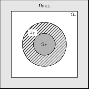
Figure 3: Cloaking of a scatterer: Optimization setting

The first example aims to minimize the visibility of an absorbing core particle $\Omega_{P}$ using optimal local orientation of an anisotropic material in the design domain $\Omega_{D}$ surrounding the particle (see Fig. 3). We assume that the background material tensor $B_{b}$ is real valued. The visibility of a scattering object can be quantified by the amount of absorbed energy and scattered energy [15]. The absorbed energy is related to the absorption cross section which is defined as

$$W^{\text{abs}}:=-\int_{\partial U}\frac{1}{2}\operatorname{Re}\left(E_{T}\times H_{T}^{*}\right)\cdot n\,\mathrm{d}\omega,$$

i. e. the total energy flow, depending on the total electric $E_{T}$ and total magnetic field $H_{T}$, through the boundary of a neighborhood $U$ of the whole scatterer $\Omega_{D}\cup\Omega_{P}$, which can be chosen, for instance, as a ball. The scattered energy is proportional to the scattering cross section which reads

$$W^{\text{sca}}:=\int_{\partial U}\frac{1}{2}\operatorname{Re}\left(E\times H^{*}\right)\cdot n\,\mathrm{d}\omega$$

with scattered field quantities $E$ and $H$. Note that both values, $W^{\text{ext}}$ and $W^{\text{sca}}$ are independent of the choice of $U$ and non-negative. Absorption and scattering can be combined into a common value, which is called the extinction cross section

$$W^{\text{ext}}:=W^{\text{abs}}+W^{\text{sca}}=\int_{\partial U}\frac{1}{2}\operatorname{Re}\left(E_{S}\times H_{I}^{*}+E_{I}\times H_{S}^{*}\right)\cdot n\,\mathrm{d}\omega.$$

This will serve as the physical objective functional $J^{p}$ in this example after a number of further adaptions. First we introduce the tensor-valued function $B_{\Omega}:\Omega\to\mathbb{S}_{\mathds{C}}$ with

$$B_{\Omega}(x)=\begin{cases}B_{C}(x)&x\in\Omega_{C}\\ B(x)&x\in\Omega_{D}.\end{cases}$$

Using transverse magnetic assumptions and switching to the two-dimensional setting, the extinction cross section transforms to

$$J^{p}(B,u)=-\operatorname{Re}\left(\frac{\imath}{2\omega}\int_{\partial U}(u^{*}_{I}(B_{\Omega}\nabla u+(B_{\Omega}-B_{b})\nabla u_{I})+u^{*}B_{b}\nabla u_{I})\cdot n\,\mathrm{d}\omega\right).$$

Moreover with partial integration and (2), we can proceed to a volume integral instead of the boundary integral and arrive at the objective functional in its final form:

(18) $$J^{p}(B,u) =-\operatorname{Re}\left(\frac{\imath}{2\omega}\int_{U}\nabla u_{I}^{H}(B_{\Omega}-B_{b})(\nabla u+\nabla u_{I})\,\mathrm{d}x\right).$$

Note that the integral in the objective functional (18) can be restricted to $\Omega_{D}\cup\Omega_{C}$.

5.1.1 Optimization problem

We collect the results from the previous sections and give the full optimization problem for this example:

$$\min_{{\boldsymbol{B}}}~{} J^{p}_{h}({\boldsymbol{B}},{\boldsymbol{u}})+\eta J^{r}_{h}({\boldsymbol{B}})+\gamma J^{g}_{h}({\boldsymbol{B}})$$

$$\operatorname{s.t.}~{} (S({\boldsymbol{B}})+S_{C}){\boldsymbol{u}}=H({\boldsymbol{B}})+H_{C}$$

$$\text{where }{\boldsymbol{B}}\text{ is parametrized by rotation angles}$$

with the objective function $J^{p}_{h}({\boldsymbol{B}},{\boldsymbol{u}})=\operatorname{Re}({\boldsymbol{u}}^{H}(V({\boldsymbol{B}})+V_{P})+W({\boldsymbol{B}})+W_{P})$ based on (18). The vectors $V({\boldsymbol{B}}),V_{P}\in\mathds{C}^{N_{p}}$ are defined element-wise as for all $1\leq i\leq{N_{p}}$

$$(V({\boldsymbol{B}}))_{i} =\frac{\imath}{2\omega}\sum_{k=1}^{{K}}\int_{T_{k}}\nabla u_{I}^{T}(B_{k}^{*}-B_{b}^{*})\nabla\varphi_{i}\,\mathrm{d}x$$

$$(V_{P})_{i} =\frac{\imath}{2\omega}\int_{\Omega_{P}}\nabla u_{I}^{T}(B_{P}^{*}-B_{b})\nabla\varphi_{i}\,\mathrm{d}x$$

and the scalars $$W({\boldsymbol{B}}),W_{P}\in\mathds{C}$$ are

$$W({\boldsymbol{B}}) =\frac{\imath}{2\omega}\sum_{k=1}^{{K}}\int_{T_{k}}\nabla u_{I}^{T}(B_{k}^{*}-B_{b}^{*})\nabla u_{I}^{*}\,\mathrm{d}x$$

$$W_{P} =\frac{\imath}{2\omega}\int_{\Omega_{P}}\nabla u_{I}^{T}(B_{P}^{*}-B^{*}_{b})\nabla u_{I}^{*}\,\mathrm{d}x.$$

Moreover, $S,S_{C},H$ and $H_{C}$ are given in Section 3.1. Together with the adjoint variable $\boldsymbol{p}$ which solves the adjoint equation

$$(S({\boldsymbol{B}})+S_{C})\boldsymbol{p}=-(V({\boldsymbol{B}})+V_{C})^{*}$$

we obtain the derivative of the physical objective functional in direction $\boldsymbol{Y}\in\mathbb{S}^{{K}}_{\mathds{C}}$ for all $k\in\mathcal{I}_{D}$

$$\frac{\mathrm{d}J^{p}_{h}({\boldsymbol{B}},{\boldsymbol{u}}({\boldsymbol{B}}))}{\mathrm{d}({\boldsymbol{B}})_{k}}[(\boldsymbol{Y})_{k}] =\operatorname{Re}\left(\int_{T_{k}}\Big{(}\nabla_{\!\!h}\boldsymbol{p}-\frac{\imath}{2\omega}\nabla u_{I}^{*}\Big{)}^{T}(\boldsymbol{Y})_{k}\Big{(}\nabla_{\!\!h}{\boldsymbol{u}}+\nabla u_{I}\Big{)}\,\mathrm{d}x\right).$$

Here, $\nabla_{\!\!h}\boldsymbol{u}=\sum_{i=1}^{N_{p}}u_{i}\nabla\varphi_{i}$ and $\nabla_{\!\!h}\boldsymbol{p}=\sum_{i=1}^{N_{p}}p_{i}\nabla\varphi_{i}$. Based on this, the sub-problems in Algorithm 1 can be established and solved using the strategies discussed in Section 4.3.1.

5.1.2 Numerical results

The particle domain $\Omega_{P}$ with material tensor $B_{P}=(0.1+2\imath)^{-2}\mathds{1}$ is a ball with radius 0.2, see Fig. 3. Inside the design domain $\Omega_{D}$, which is a ball with radius 0.4, the material tensor is optimized with rotational parametrization based on the diagonal reference material tensor $B^{(r)}=\operatorname{diag}(1,2)^{-2}$. A box with a side length of 2 defines $\Omega_{b}$ and a layer with thickness 1 represents the PML both with material properties $B_{b}=\mathds{1}$.

Furthermore, we choose a plane incident wave $u_{I}(x,y)=\sqrt{2}\exp(\imath\omega x)$ with wavelength $\lambda=0.55,\omega=\frac{2\pi}{\lambda}$ and set the PML function to $s(t)=1-\frac{100}{\imath\omega}\max(0,|t|-1)$.

The state and adjoint equation are solved using the Finite Element Method (FEM) on triangluar cells and implemented in MATLAB [14]. We use linear Lagrange basis functions [27] to approximate the scalar fields. The triangulation of the computational domain is generated with the Delaunay triangulation tool Triangle [20] and the triangulation process provides approx. $1\text{\times}{10}^{5}$ triangular elements in total and approx. $3\text{\times}{10}^{4}$ triangles in the design region $\Omega_{D}$.

Since in this example we consider a rotational parametrization (Definition 4.22), the admissible set is given as $\mathcal{B}=\mathcal{G}^{K}$ with $\mathcal{G}=\{R(\pi\delta)B^{(r)}R(\pi\delta)^{T}\mid\delta\in[0,1]\}$. Thus the underlying graph has only one closed edge. The asymptotes for Algorithm 1 are defined by $l=0$ and $u=100$ and thus satisfy the assumptions in Definition 4.2. We choose the regularization parametrer $\eta=100$, the circular filter radius $r_{0}=0.01$ and the grayness penalty factor $\gamma=0$.

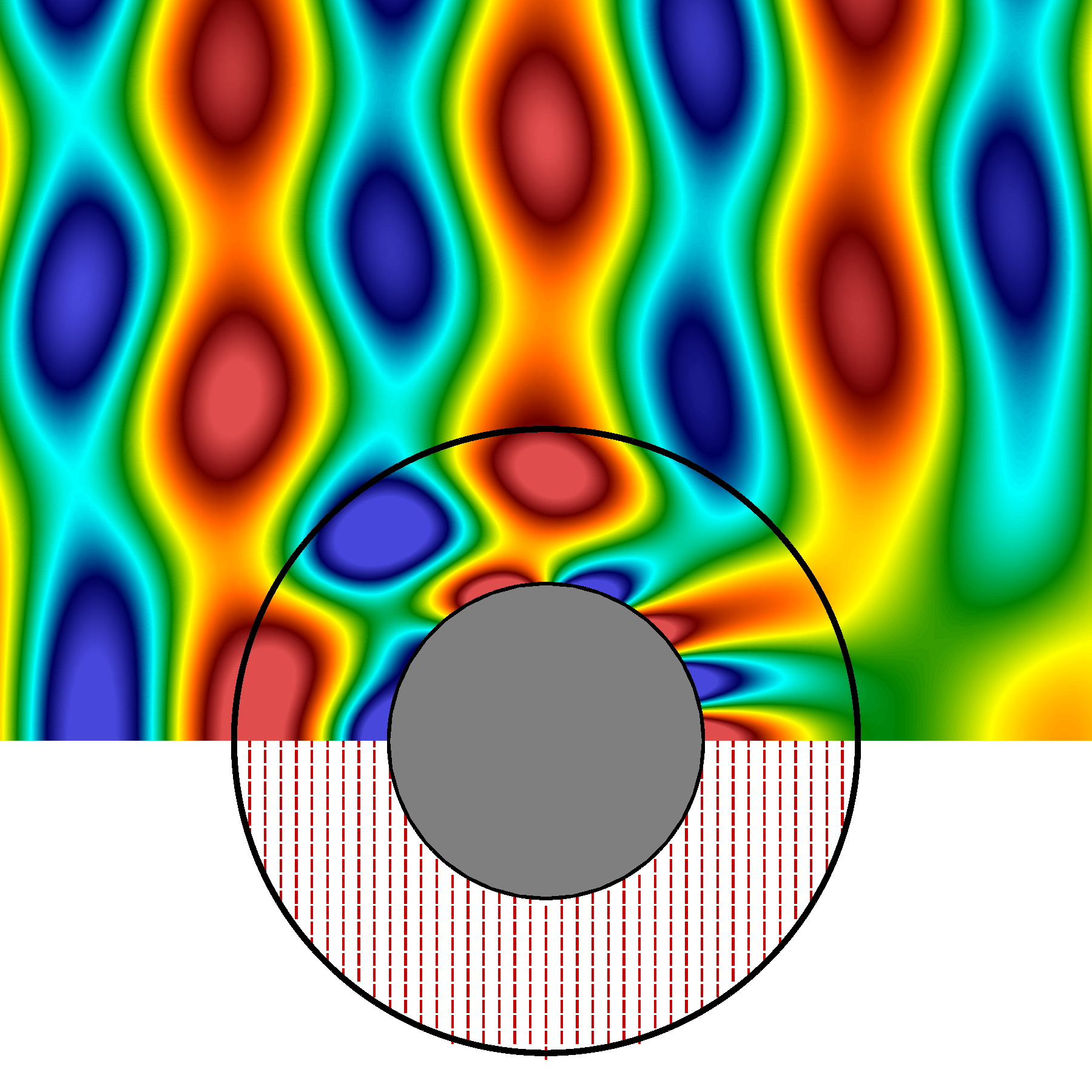
(a) inital

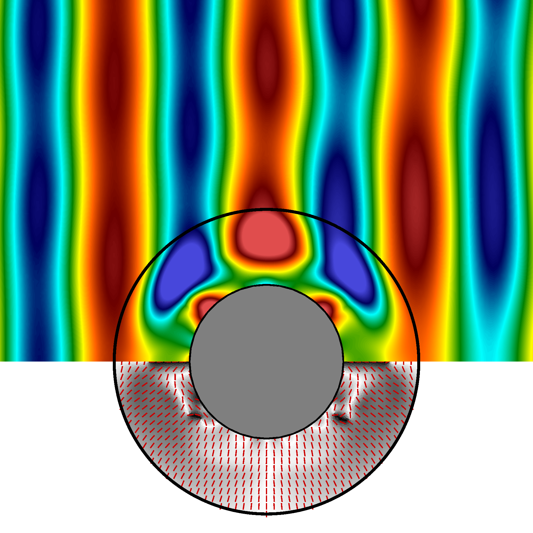
(b) optimized

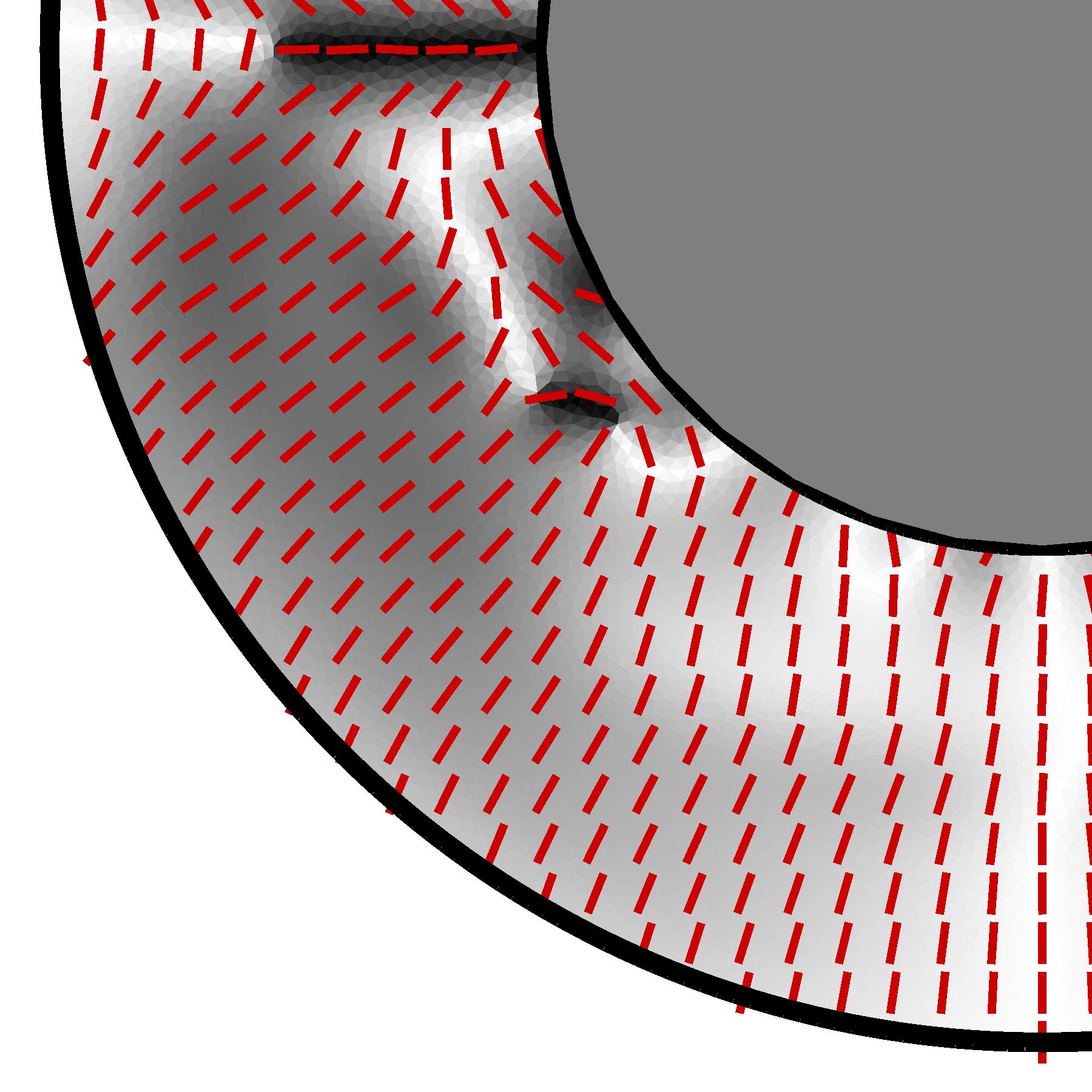
(c) close-up

Figure 4: Optimization result for the cloaking of scatterer with anisotropic material

In the upper part of Fig. 4(a) and Fig. 4(b) the total magnetic field is illustrated for the initial and the optimal design configuration, respectively. The backscattering and absorption of the particle including the coating layer is clearly visible for the initial configuration. In the lower section of both figures the local orientation of the anisotropic tensor inside the coating layer is visualized. The gray scale colors represent the absolute value of the orientation angle between $0$ and $\frac{\pi}{2}$ and the dashes in the closeup (see Fig. 4(c)) support the illustration of the orientation angle. The extinction cross section associated with the optimized anisotropic coating layer is decreased by over $88$ relative to the initial design.

As previously mentioned, we are also interested in the performance of Algorithm 1, if we restrict the design to $L\in\mathds{N}$ uniformly distributed admissible orientations, i. e. $\tfrac{\pi l}{L}$ for all $0\leq l\leq L-1$. In order to investigate this, the underlying graph of $\mathcal{G}$ is divided into $L$ edges, i. e. ${N_{E}}=L$, and we obtain the modified admissible set $\mathcal{B}$ with

$$\mathcal{G}=\bigcup_{l=0}^{L-1}\left\{R\left(\tfrac{\pi}{L}(\delta+l)\right)B^{(r)}R\left(\tfrac{\pi}{L}(\delta+l)\right)^{T}\mid\delta\in[0,1]\right\}$$

and $\mathcal{N}=\{R\left(\tfrac{\pi l}{L}\right)B^{(r)}R\left(\tfrac{\pi l}{L}\right)^{T}\mid 0\leq l\leq L-1\}$. To ensure that only points located at nodes are considered, in theory we could choose a penalty parameter $\gamma>\gamma_{\text{max}}$. However, as we know from Remark 4.20 that the global minimizer of each sub-problem is located in the set $\mathcal{N}^{K}$ in this case, rather than solving the sub-problem as described in Section 4.3.2, we can evaluate the model objective in all nodes and choose the one with the lowest function value for each element.

Table 1: Progression of the relative cloaking with respect to number of admissible angles

number of angles	rel. cloaking
4	85.69
12	41.35
18	36.71
60	27.05
180	19.80
360	12.73
continuous	11.86

The relative cloaking after optimization with different numbers of admissible angles is listed in Table 1. It can be observed that with an increasing number of orientations, the optimal value of the cost function approaches the optimal value of the continuous problem. This reveals that despite the apparent ’brute force’ approach to the solution of the sub-problem, the algorithm is obviously not trapped in local optima introduced by the highly non-convex grayness terms.

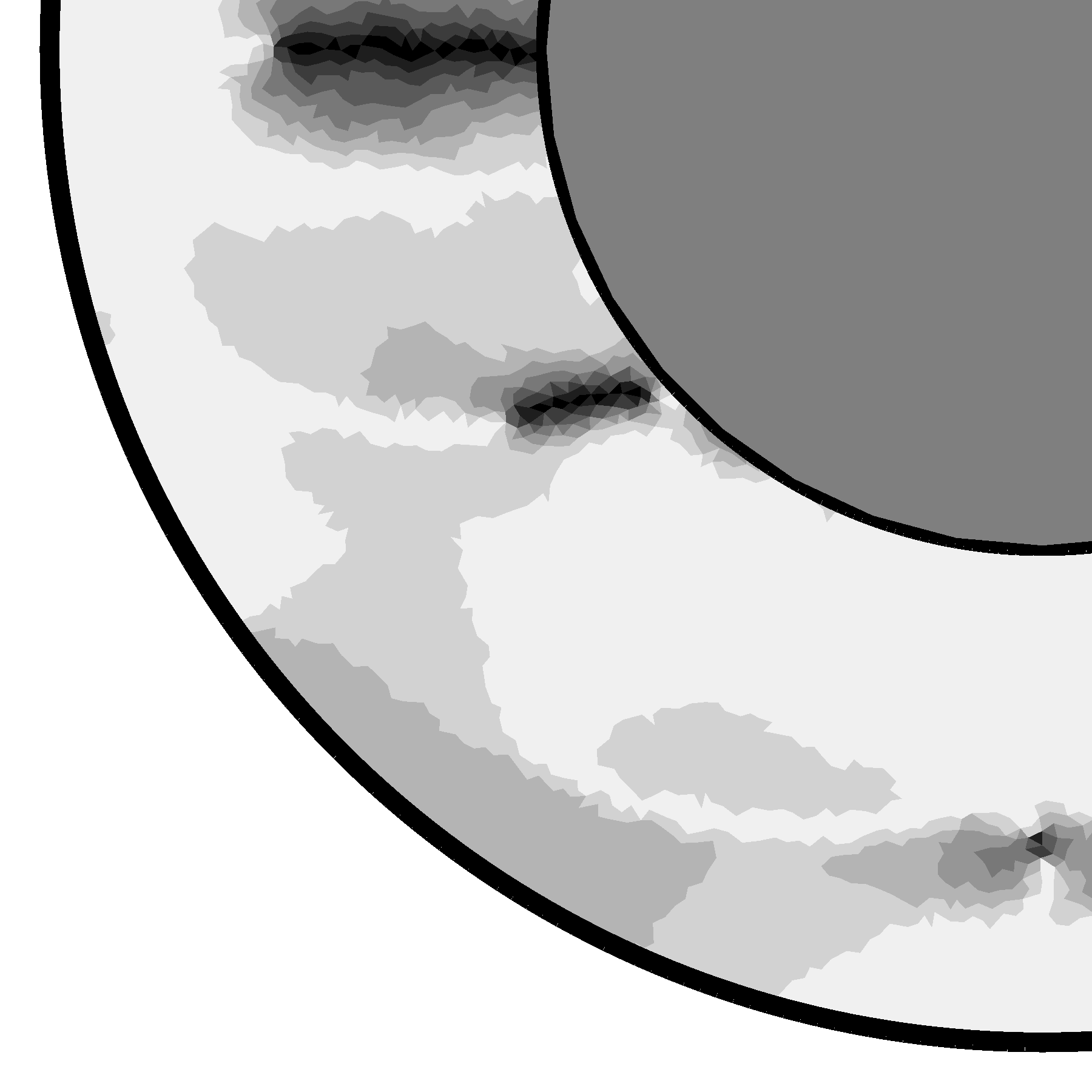
(a) 18 angles

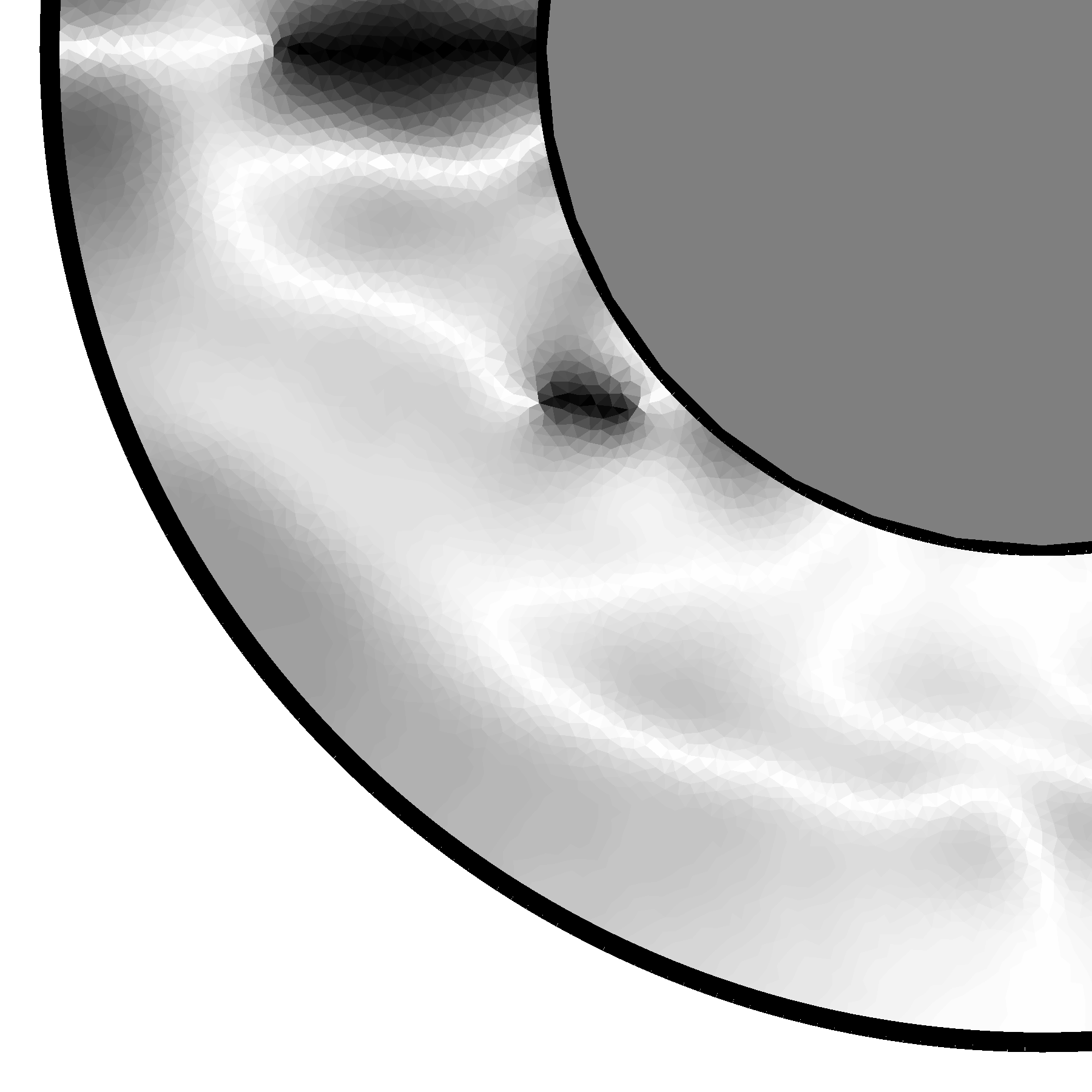
(b) 180 angles

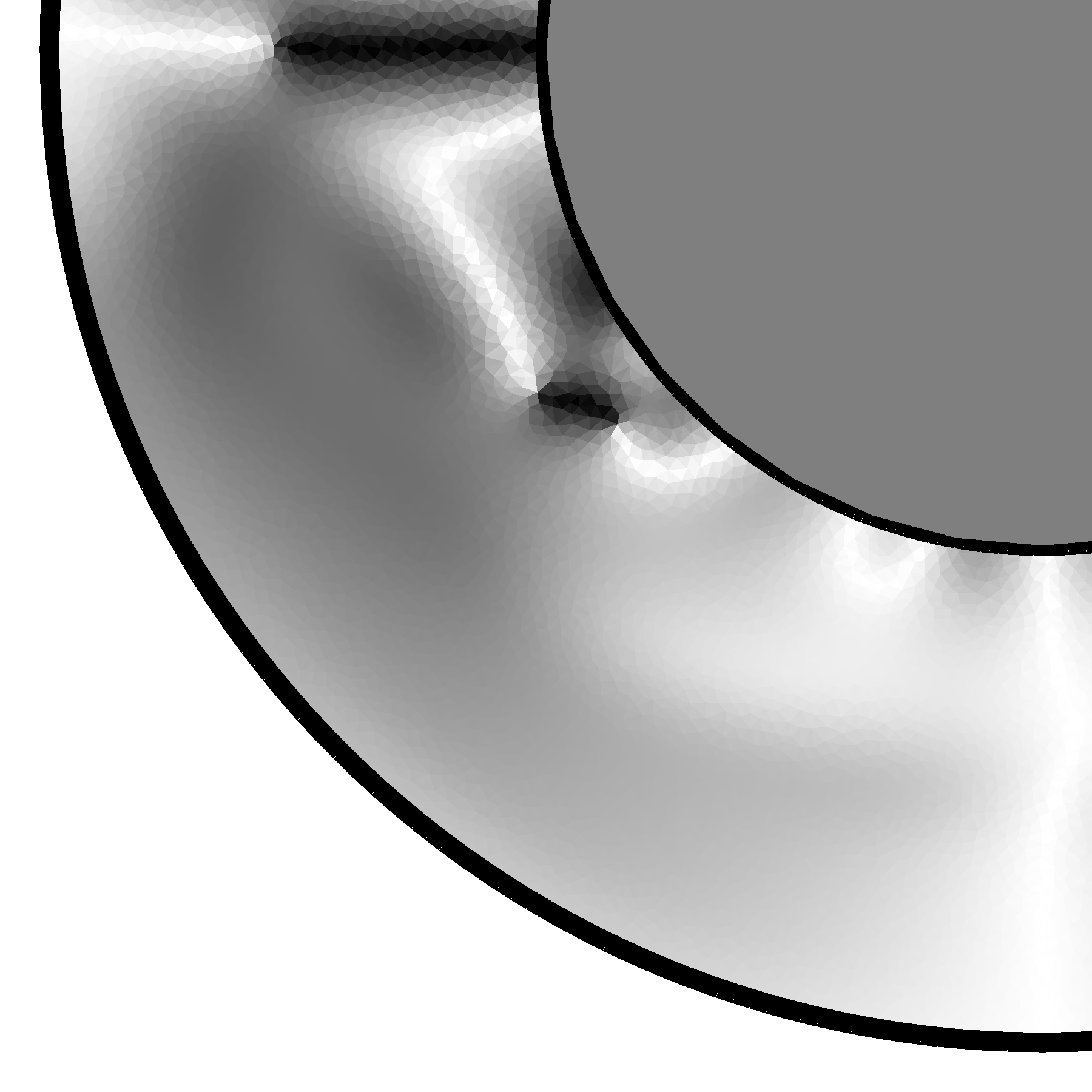
(c) continuous

Figure 5: Comparison of optimization results for different number of admissible orientations

In Fig. 5 the close up of the optimization results for 18 admissible angle, 180 admissible angles and the continuous setting are compared.

5.2 Tomographic reconstruction

In this example we attempt to reconstruct a known material distribution by using the electromagnetic field response on the artificial observation boundary $\partial U$. To do this, we define the physical objective functional following [4, 26] as

$$J^{p}(u;u_{D})=\int_{\partial U}|u(x)-u_{D}(x)|^{2}\,\mathrm{d}x.$$

The objective functional measures the distance of a magnetic field $u:\Omega\to\mathds{C}$ associated with a material configuration $B$ to the magnetic field $u_{D}:\Omega\to\mathds{C}$ associated with a reference configuration $B_{D}$ on the observation boundary $\partial U$. After discretization, we obtain

$$J^{p}_{h}({\boldsymbol{u}};u_{D})=\operatorname{Re}\left({\boldsymbol{u}}^{H}Q{\boldsymbol{u}}+2{\boldsymbol{u}}^{H}V(u_{D})+W(u_{D})\right)$$

where $Q\in\mathds{R}^{{N_{p}}\times{N_{p}}},V(u_{d})\in\mathds{C}^{{N_{p}}}$ and $W(u_{D})\in\mathds{R}$ are defined element-wise for all $1\leq i,j\leq{N_{p}}$ by

$$(Q)_{ij} :=\int_{\partial U}\varphi_{i}\varphi_{j}\,\mathrm{d}x, (V(u_{D}))_{i} :=\int_{\partial U}\varphi_{i}u_{D}\,\mathrm{d}x, W(u_{D}) :=\int_{\partial U}|u_{D}|^{2}\,\mathrm{d}x.$$

This functional must be minimized for multiple incident plane waves $u_{I}(x;\omega,d)=\exp(\imath\omega d\cdot x)$ depending on wave number $\omega$ and direction $d$. Hence, let ${N_{\omega}}$ wave numbers $\omega_{1},\dotsc,\omega_{N_{\omega}}$ and ${N_{d}}$ directions $d_{1},\dotsc,d_{N_{d}}$ be given, then the physical objective functional for multiple incident waves $\boldsymbol{J}^{p}_{h}$ is

$$\boldsymbol{J}^{p}_{h}({\boldsymbol{u}}^{11},\dotsc,{\boldsymbol{u}}^{{N_{\omega}}{N_{d}}})=\sum_{l=1}^{N_{\omega}}\sum_{m=1}^{N_{d}}J^{p}_{h}({\boldsymbol{u}}^{lm};u^{lm}_{D})$$

where ${\boldsymbol{u}}^{lm}$ is the solution of the state equation for wave number $\omega_{l}$, incident direction $d_{m}$ with incident wave $u_{I}(x)=u_{I}(x;\omega_{l},d_{m})$ and $u^{lm}_{D}$ is the corresponding reference solution, i. e. $u_{D}^{lm}(x)=u_{D}(x;\omega_{l},d_{m})$.

5.2.1 Optimization problem

We again gather the results of the previous sections, and extend the optimization problem (2) to multiple incident waves:

$$\left\{\qquad\begin{aligned} \min_{{\boldsymbol{B}}}~{}&\boldsymbol{J}^{p}_{h}({\boldsymbol{u}}^{11},\dotsc,{\boldsymbol{u}}^{{N_{\omega}}{N_{d}}})+\eta J^{r}_{h}({\boldsymbol{B}})+\gamma J^{g}_{h}({\boldsymbol{B}})&\\ \operatorname{s.t.}~{}&(S({\boldsymbol{B}})+S_{C}){\boldsymbol{u}}^{lm}=(H({\boldsymbol{B}})+H_{C})\\ &\text{with }\omega=\omega_{l}\text{ and }u_{I}(x)=u_{I}(x;w_{l},d_{m})\\ &\text{where }{\boldsymbol{B}}\text{ is parametrized using polynomial interpolations}\end{aligned}\right.$$

With $\boldsymbol{p}^{lm}\in\mathds{C}^{N_{p}}$ solving the adjoint equation

$$(S({\boldsymbol{B}})+S_{C})\boldsymbol{p}^{lm} =-2(Q{\boldsymbol{u}}^{lm}+L(u^{lm}_{D}))^{*}$$

for $\omega=\omega_{l}$, we are once more able to give a formula for the derivative of the physical objective in direction $\boldsymbol{Y}\in\mathbb{S}^{{K}}_{\mathds{C}}$ for all $k\in\mathcal{I}_{D}$ as follows:

$$\frac{\mathrm{d}\boldsymbol{J}^{p}_{h}({\boldsymbol{u}}^{11},\dotsc,{\boldsymbol{u}}^{{N_{\omega}}{N_{d}}})}{\mathrm{d}({\boldsymbol{B}})_{k}}[(\boldsymbol{Y})_{k}] =\sum_{l=1}^{N_{\omega}}\sum_{m=1}^{N_{d}}\operatorname{Re}\left(\int_{T_{k}}(\nabla_{\!\!h}{\boldsymbol{u}}^{lm}+\nabla u_{I}^{lm})^{T}(\boldsymbol{Y})_{k}\nabla_{\!\!h}\boldsymbol{p}^{lm}\,\mathrm{d}x\right).$$

As in the previous example, we have used $\nabla_{\!\!h}\boldsymbol{u}=\sum_{i=1}^{N_{p}}u_{i}\nabla\varphi_{i}$, $\nabla_{\!\!h}\boldsymbol{p}=\sum_{i=1}^{N_{p}}p_{i}\nabla\varphi_{i}$ and additionally $u_{I}^{lm}(x)=u_{I}(x;\omega_{l},d_{m})$. With this as a basis, again sub-problems can be formulated and solved using the techniques described in Section 4.3.2.

5.3 Numerical Results

The design domain $\Omega_{D}$ is a ball with radius $0.4$ and is contained in a square with side length $2$. Furthermore a perfectly matched layer of thickness $1$ is used and the PML function $s(t)$ is defined as in the previous example. The scattered electromagnetic field $u_{D}$ of the reference configuration $B_{D}$ is calculated on the same mesh, but perturbed at every spatial point with a weighted normal probability density function with mean value $0$ and variance $1$. The reference magnetic field $u_{D}$ is used for the evaluation of the objective function on the observation boundary defined by a sphere with radius $0.8$. Furthermore, the scatterer is illuminated from $8$ directions in $45\text{\,}\mathrm{\SIUnitSymbolDegree}$ steps and $8$ uniformly distributed wavelengths in the interval $[0.4,0.7]$.

The set of admissible material tensors is the cyclic graph with three edges ($\mathcal{I}_{E}=\{1,\dotsc,3\}$) and linear interpolation of the isotropic materials $B^{(1)}=\mathds{1}$, $B^{(2)}=(2)^{-2}\mathds{1}$ and $B^{(3)}=(1+2\imath)^{-2}\mathds{1}$.

(a) material distribution $B_{D}$

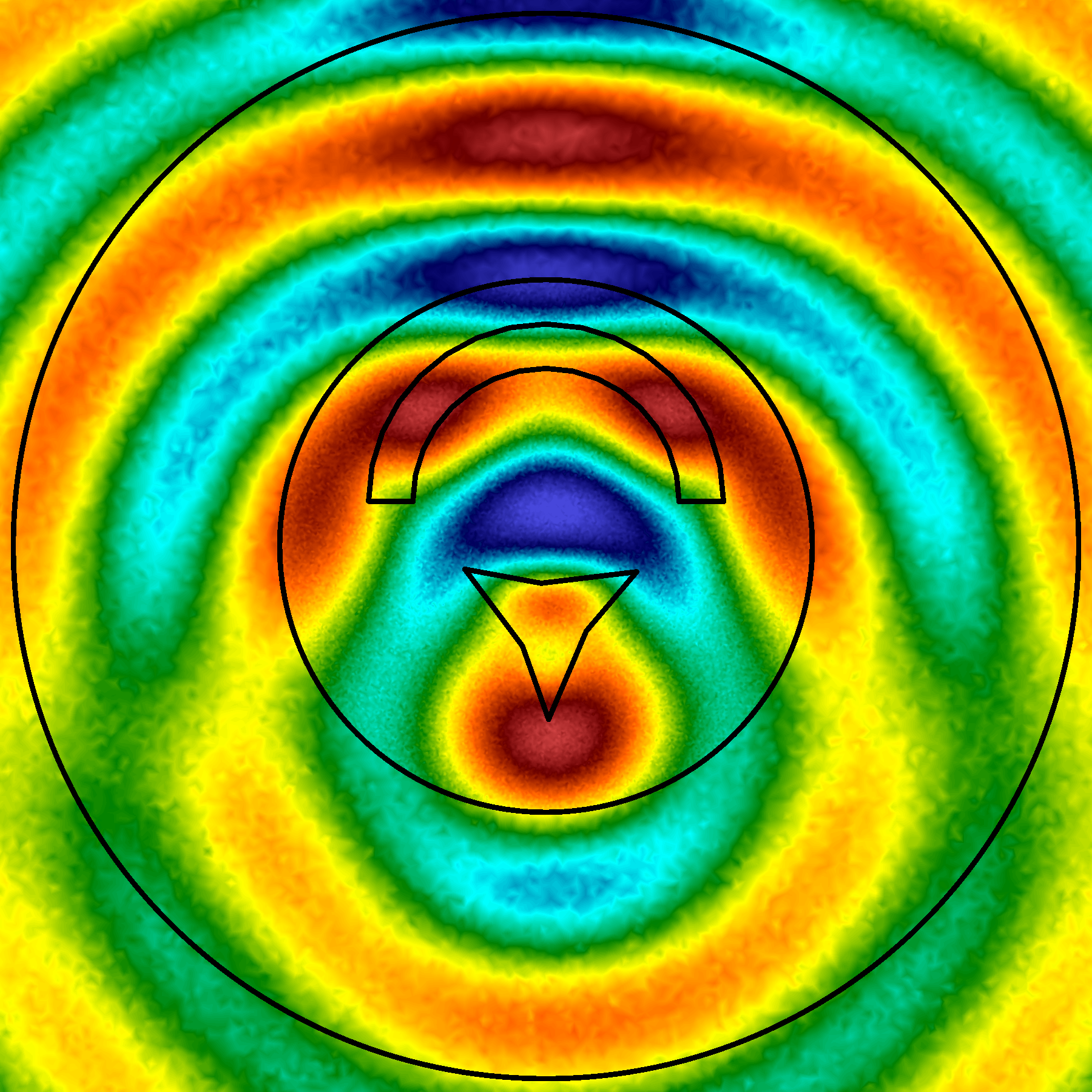
(b) noisy scattered target field $u_{D}$

Figure 6: Reference material configuration and reference magnetic field including noise.

Fig. 6(a) illustrates the material distribution $B_{D}$ inside the circular design domain, where white corresponds to $B^{(1)}$, green corresponds to $B^{(2)}$ and red corresponds to $B^{(3)}$, respectively. Moreover the outline of the design domain and material distribution is marked by black lines. The noisy scattered magnetic field for a fixed wavelength and illumination direction is depicted in Fig. 6(b). Here, the outermost circle is the observation boundary $\partial U$ where the objective functional is evaluated.

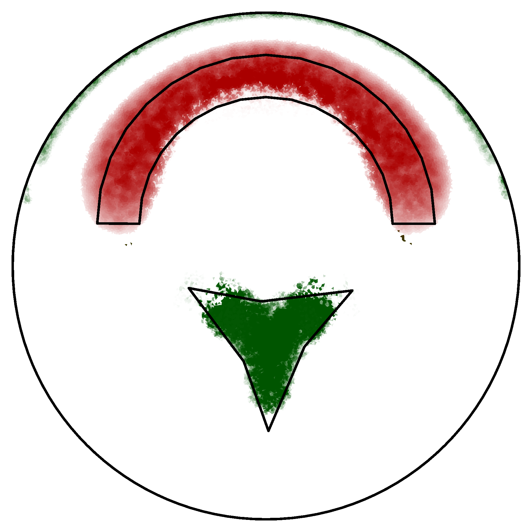
(a) $\eta=0.1$

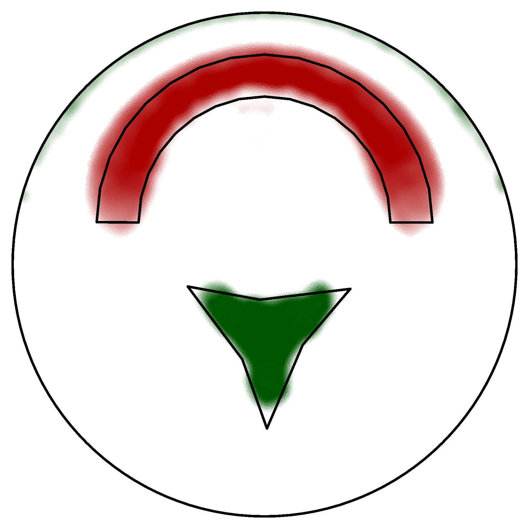
(b) $\eta=1$

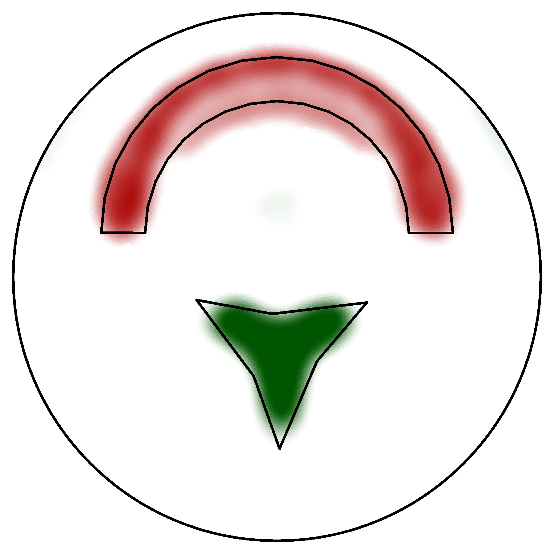
(c) $\eta=10$

Figure 7: Effect of filter penalization factor $\eta$ on optimization result after 100 iterations, $\gamma=${10}^{-6}$$, $r_{0}=0.01$, colored by material index

First we wish to analyze the influence of the regularization. We set the circular filter radius to $r_{0}=0.01$, choose a grayness parameter of $\gamma=${10}^{-6}$$ and perform the optimization with various choices of regularization constants $\eta\in\{$0.1$,$1$,$10$\}$. In Fig. 7, the optimization result after 100 iterations is depicted for all choices; the effect of the regularization becomes apparent at the blurred interfaces. While the influence of the filter radius was also studied, this is not described here.

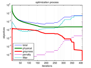
(a) objective functional

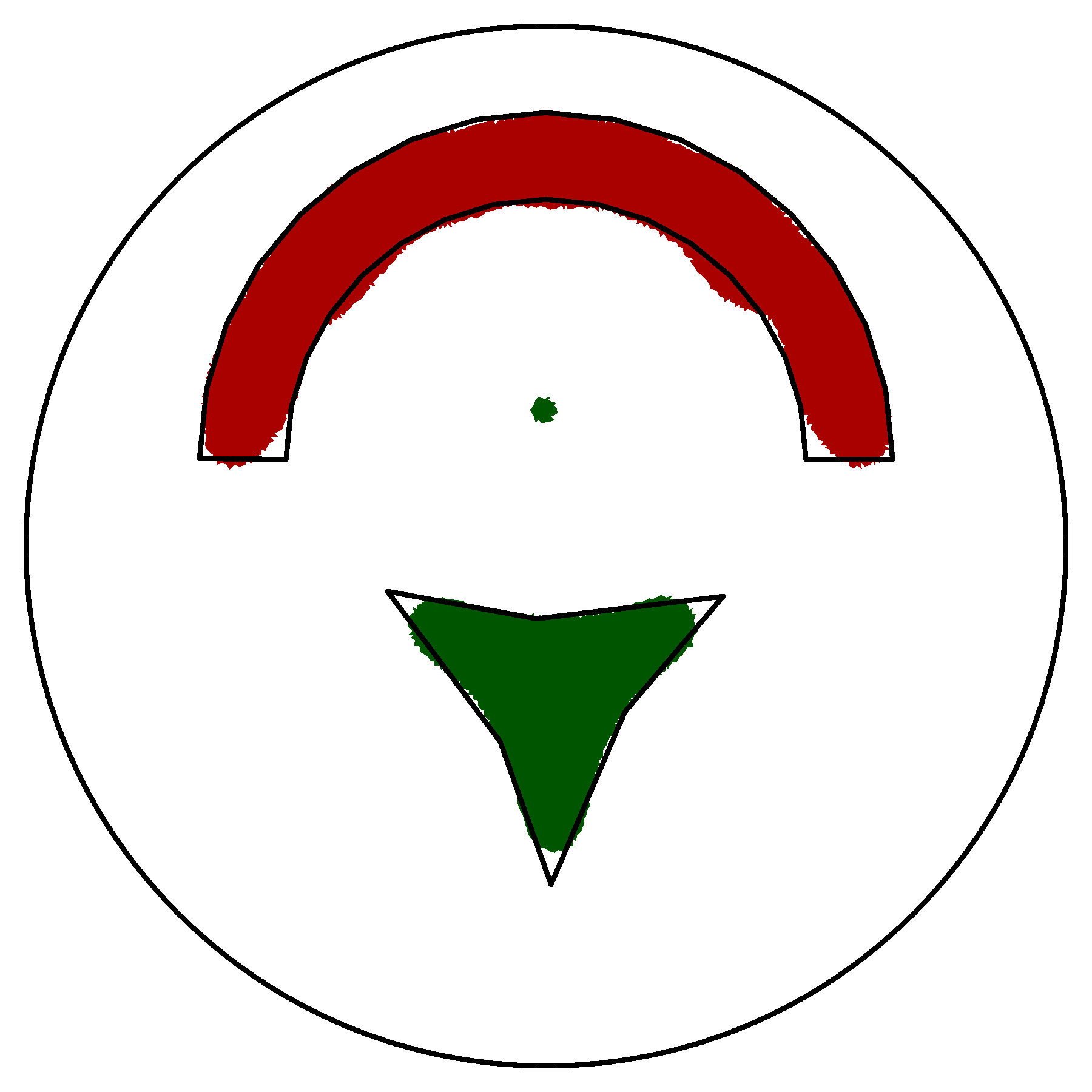
(b) optimization result

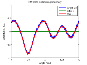
(c) magnetic field on $\partial U$

Figure 8: Evolution of the objective functional with continuation procedure and magnetic field quantities on the observation boundary $\partial U$ for single wavelength and illumination direction

During the final optimization process, a continuation procedure like that in [22] was executed, i. e. the algorithm was repeatedly restarted with an increased grayness penalty factor $\gamma$ and the previous optimization result as starting point. Based on the previous investigations we fixed $\eta=1$ and $r_{0}=0.01$, and initialized the material tensor in the design domain with background material. In Fig. 8(a) the evolution of the objective functional value, normalized to the inital state, is depicted. The objective functional (total) is composed of the extinctional cross section $\boldsymbol{J}^{p}_{h}$ (physical), the regularization term $J^{r}_{h}$ (filter) and the grayness term $J^{g}_{h}$ (grayness); all contributions are plotted seperately. Due to the increment of the grayness penalty factor $\gamma$ (penalty), the total objective functional increases but the physical and grayness contributions decrease successively. Additionally, the vertical lines in Fig. 8(a) mark the continuation procedure where either a predefined maximum number of iterations is exceeded or a stopping criterion is reached. The continuation process is ended when a so-called black/white solution ($J^{g}_{h}=0$) is achieved. Thus, we finally obtain a material distribution with tensor values corresponding to the nodes of the underlying graph (Fig. 8(b)). The difference between the target and optimized magnetic response, i. e. the physical objective functional, drops to $0.2$. This can be also qualitively observed in Fig. 8(c), where for a single wavelength and illumination direction the magnetic response $u$ and the noisy target field $u_{D}$ are compared along the circular observation boundary $\partial U$.

Finally, we study the effect of the filter penalization on the optimization result in combination with the continuation strategy. Fig. 9 depicts the results of the optimization with continuation process, where the filter penalty factor $\eta\in\{0.1,10,100\}$ is varied. It is evident that the overall shape of the scatterer has been more or less reconstructed. For the smallest factor $\eta=0.1$, we see a ragged boundary, whereas for the largest factor $\eta=100$ the filtering was too strong and dominated the tracking objective.

In all cases the sharp features, like the edges of the star, are poorly reconstructed, which may be caused by the low number of wavelengths and illumination directions.

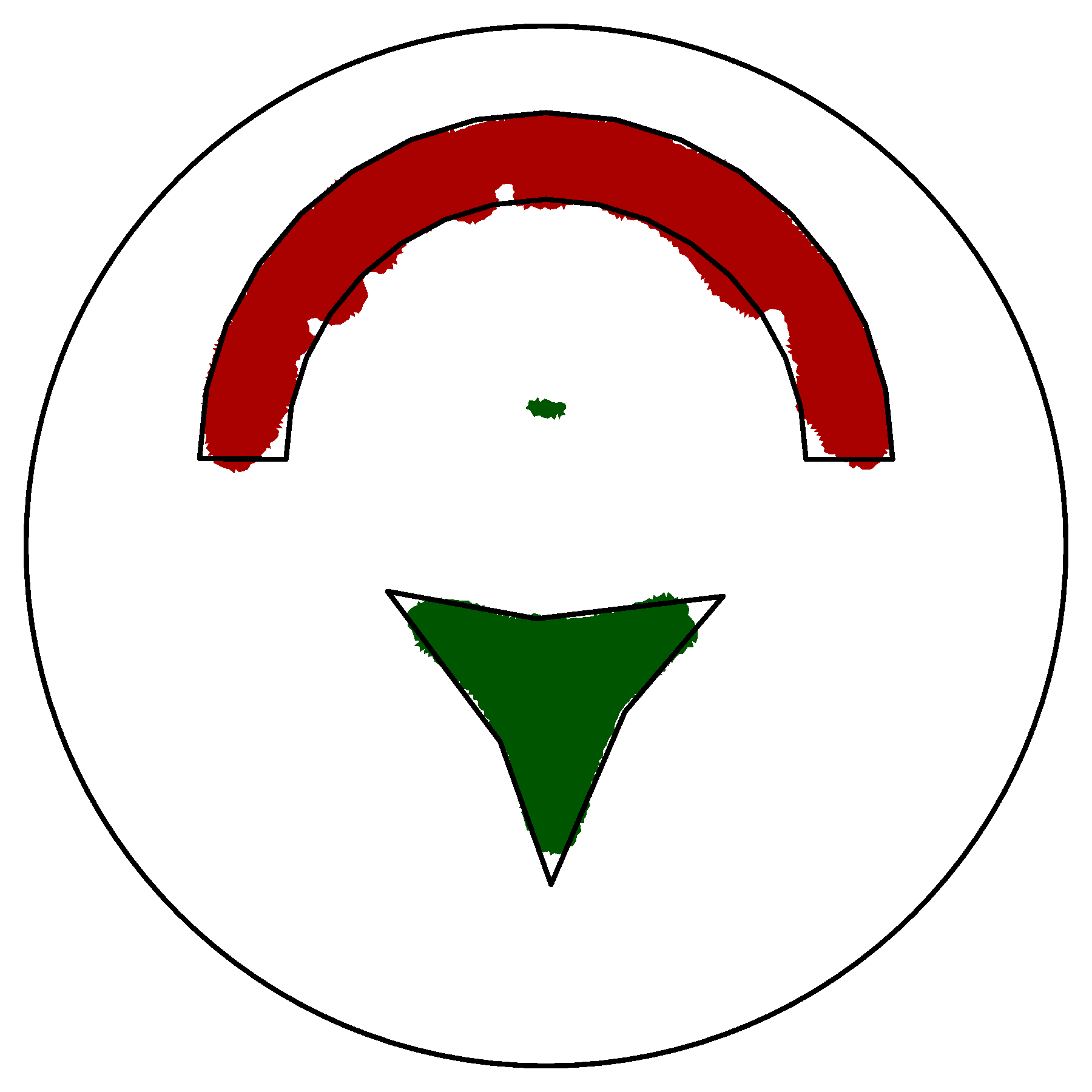
(a) $\eta=0.1$

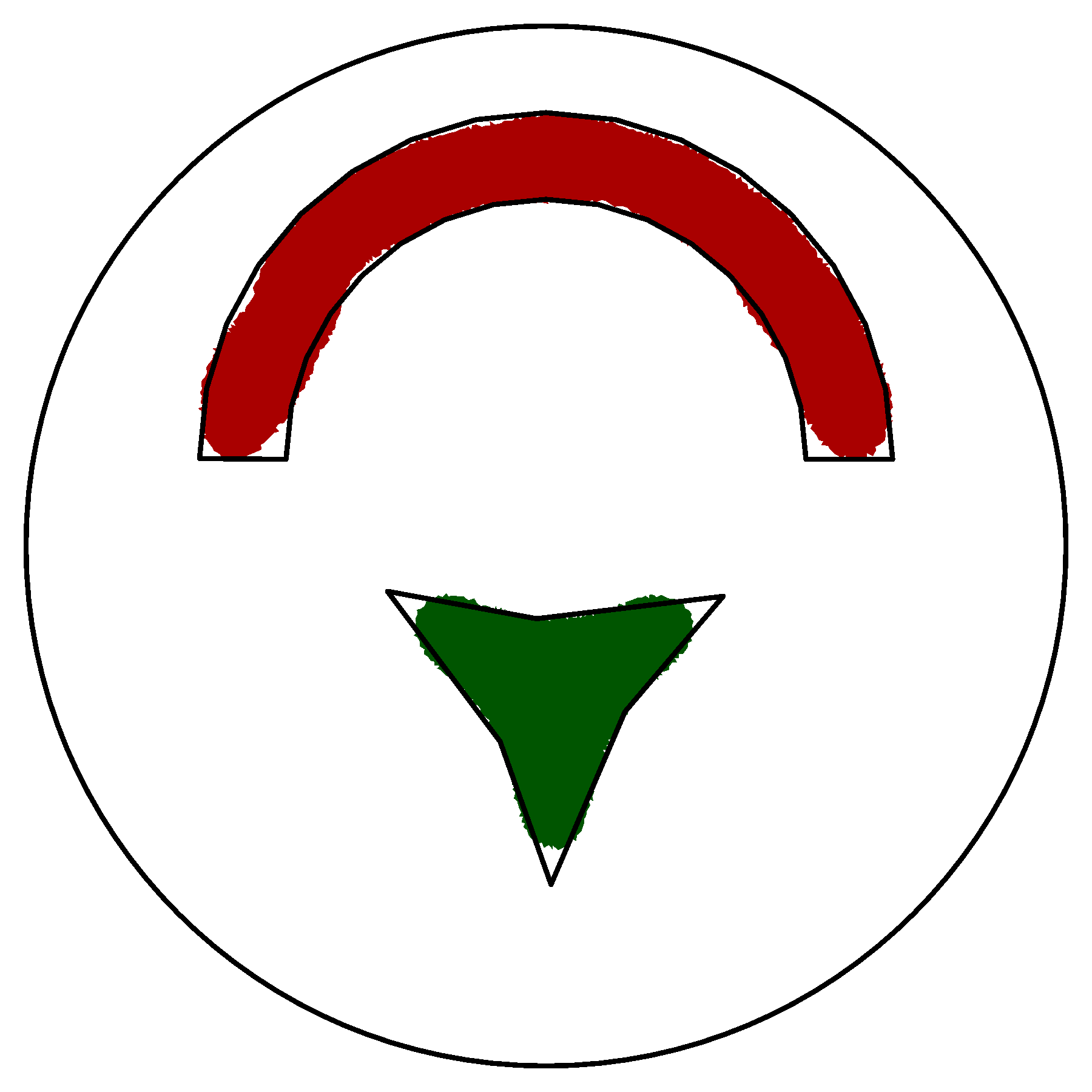
(b) $\eta=10$

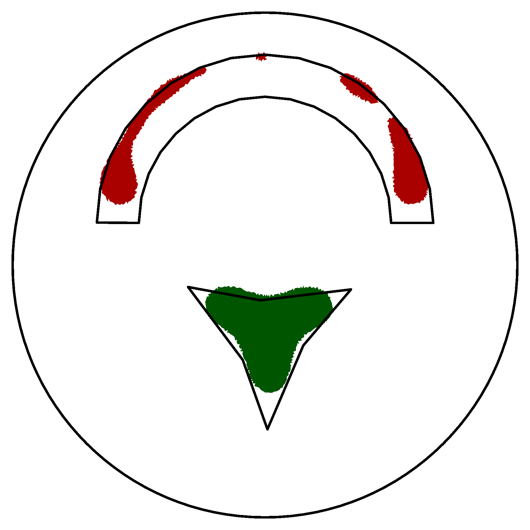
(c) $\eta=100$

Figure 9: Optimization result with variation of the filter penalty $\eta$

6 Concluding Remarks

We have proposed a new algorithm for the solution of material optimization problems in electromagnetics. The algorithm is flexible in the sense that it can be applied to material problems of a discrete and continuous nature. Theoretical properties of the algorithm such as global convergence have been discussed and it was further shown in the course of numerical experiments that poor local optima introduced by seriously non-linear parametrizations can be avoided. An open question remains: how can the improvement of the new algorithm over the application of general purpose optimization algorithms be quantified? This will be investigated in the near future, based on extended numerical experiments and a thorough mathematical investigation of the properties of limit points. In terms of the application side it would be a natural next step to apply the concept to three dimensional problems and to consider efficient parallelization. The algorithmic concept discussed in the article seems particularly suited for the latter due to the block separable structure of the sub-problem, which must be solved in each major iteration.

References

- [1] M. P. Bendsøe, J. M. Guedes, R. B. Haber, P. Pedersen, and J. E. Taylor, An Analytical Model to Predict Optimal Material Properties in the Context of Optimal Structural Design, J. Appl. Mech., 61 (1994), p. 930.
- [2] J. P. Berenger, A perfectly matched layer for the absorption of electromagnetic waves, J. Comput. Phys., 114 (1994), pp. 185–200.
- [3] J.-K. Byun, J.-H. Lee, and I.-H. Park, Node-Based Distribution of Material Properties for Topology Optimization of Electromagnetic Devices, IEEE Trans. Magn., 40 (2004), pp. 1212–1215.
- [4] M. Cheney, D. Isaacson, and J. C. Newell, Electrical Impedance Tomography, SIAM Rev., 41 (1999), pp. 85–101.
- [5] A. R. Diaz and O. Sigmund, A topology optimization method for design of negative permeability metamaterials, Struct. Multidiscip. Optim., 41 (2010), pp. 163–177.
- [6] A. Edelman and H. Murakami, Polynomial roots from companion matrix eigenvalues, Math. Comput., 64 (1995), pp. 763–763.
- [7] P. E. Gill, W. Murray, and M. A. Saunders, SNOPT: An SQP Algorithm for Large-Scale Constrained Optimization, SIAM J. Optim., 12 (2002), pp. 979–1006.
- [8] J. Greifenstein and M. Stingl, Simultaneous parametric material and topology optimization with constrained material grading, Struct. Multidiscip. Optim., 54 (2016), pp. 985–998.
- [9] R. B. Haber, C. S. Jog, and M. P. Bendsoe, A new approach to variable-topology shape design using a constraint on perimeter, Struct. Optim., 11 (1996), pp. 1–12.
- [10] E. Hassan, E. Wadbro, and M. Berggren, Topology Optimization of Metallic Antennas, IEEE Trans. Antennas Propag., 62 (2014), pp. 2488–2500.
- [11] C. F. Hvejsel and E. Lund, Material interpolation schemes for unified topology and multi-material optimization, Struct. Multidiscip. Optim., 43 (2011), pp. 811–825.
- [12] J. D. Jackson, Classical Electrodynamics, Wiley, New York, 3rd ed., 2004.
- [13] O. Kwon, E. J. Woo, J.-R. Yoon, and J. K. Seo, Magnetic resonance electrical impedance tomography (MREIT): simulation study of J-substitution algorithm, IEEE Trans. Biomed. Eng., 49 (2002), pp. 160–167.
- [14] MATLAB, v8.3.0.532 (R2014a), The MathWorks Inc., Nantick, Massachusetts, United States, 2014.
- [15] M. I. Mishchenko, Electromagnetic Scattering by Particles and Particle Groups: An Introduction, Cambridge University Press, Cambridge, 2014.
- [16] P. Monk, Finite Element Methods for Maxwell’s Equations, Clarendon Press, Oxford; New York, 1st ed., 2003.
- [17] P. Pedersen, On optimal orientation of orthotropic materials, Struct. Optim., 1 (1989), pp. 101–106.
- [18] J. B. Pendry, Controlling Electromagnetic Fields, Science (80-. )., 312 (2006), pp. 1780–1782.
- [19] U. T. Ringertz, On finding the optimal distribution of material properties, Struct. Optim., 5 (1993), pp. 265–267.
- [20] J. R. Shewchuk, Triangle: Engineering a 2D quality mesh generator and Delaunay triangulator, in Appl. Comput. Geom. Towar. Geom. Eng., vol. 1148, Springer, Berlin; Heidelberg, 1996, pp. 203–222.
- [21] O. Sigmund, On the Design of Compliant Mechanisms Using Topology Optimization, Mech. Struct. Mach., 25 (1997), pp. 493–524.
- [22] O. Sigmund and J. Petersson, Numerical instabilities in topology optimization: A survey on procedures dealing with checkerboards, mesh-dependencies and local minima, Struct. Optim., 16 (1998), pp. 68–75.
- [23] J. Stegmann and E. Lund, Discrete material optimization of general composite shell structures, Int. J. Numer. Methods Eng., 62 (2005), pp. 2009–2027.
- [24] M. Stingl, M. Kočvara, and G. Leugering, A Sequential Convex Semidefinite Programming Algorithm with an Application to Multiple-Load Free Material Optimization, SIAM J. Optim., 20 (2009), pp. 130–155.
- [25] K. Svanberg, The method of moving asymptotes—a new method for structural optimization, Int. J. Numer. Methods Eng., 24 (1987), pp. 359–373.
- [26] M. Vauhkonen, D. Vadasz, P. Karjalainen, E. Somersalo, and J. Kaipio, Tikhonov regularization and prior information in electrical impedance tomography, IEEE Trans. Med. Imaging, 17 (1998), pp. 285–293.
- [27] O. Zienkiewicz, R. Taylor, and J. Zhu, The finite element method: its basis and fundamentals, Elsevier, Amsterdam; Boston; Heidelberg, 6th ed., 2005.
- [28] J. Zowe, M. Kočvara, and M. P. Bendsøe, Free material optimization via mathematical programming, Math. Program., 79 (1997), pp. 445–466.