Spatial Filtering for Reduced Order Modeling

1. Introduction

Spatial filtering has been central in the development of large eddy simulation reduced order models (LES-ROMs) [8, 10, 11] and regularized reduced order models (Reg-ROMs) [6, 9] for efficient and relatively accurate numerical simulation of convection-dominated fluid flows. In this paper, we perform a numerical investigation of spatial filtering. To this end, we consider one of the simplest Reg-ROMs, the Leray ROM (L-ROM) [6, 9], which uses ROM spatial filtering to smooth the flow variables and decrease the amount of energy aliased to the lower index ROM basis functions. We also propose a new form of ROM differential filter [6, 9] and use it as a spatial filter for the L-ROM. We investigate the performance of this new form of ROM differential filter in the numerical simulation of a flow past a circular cylinder at a Reynolds number $Re=760$.

2. Reduced Order Modeling

For the Navier-Stokes equations (NSE), the standard reduced order model (ROM) is constructed as follows: (i) choose modes $\{\vec{\varphi}_{1},\ldots,\vec{\varphi}_{d}\}$, which represent the recurrent spatial structures of the given flow; (ii) choose the dominant modes $\{\vec{\varphi}_{1},\ldots,\vec{\varphi}_{r}\}$, $r\leq d$, as basis functions for the ROM; (iii) use a Galerkin truncation $\vec{u}_{r}=\sum_{j=1}^{r}a_{j}\,\vec{\varphi}_{j}$; (iv) replace $\vec{u}$ with $\vec{u}_{r}$ in the NSE; (iii) use a Galerkin projection of NSE($\vec{u}_{r}$) onto the ROM space $X^{r}:=\mbox{span}\{\vec{\varphi}_{1},\ldots,\vec{\varphi}_{r}\}$ to obtain a low-dimensional dynamical system, which represents the ROM:

(1) $$\dot{\vec{a}}=A\,\vec{a}+\vec{a}^{\top}\,B\,\vec{a}\,,$$

where $\vec{a}$ is the vector of unknown ROM coefficients and $A,B$ are ROM operators; (iv) in an offline stage, compute the ROM operators; and (v) in an online stage, repeatedly use the ROM (for various parameter settings and/or longer time intervals).

3. ROM Differential Filter

The ROM differential filter is based on the classic Helmholtz filter that has been used to great success in LES for turbulent flows [3]. Let $\delta$ be the radius of the differential filter. Then, for a given velocity field $\vec{u}_{r}\in X^{r}$, the filtered flow field $\mathcal{F}(\vec{u}_{r})\in X^{f}$, where $X^{f}$ is a yet to be specified space of filtered ROM functions, is defined as the solution to the Helmholtz problem

(2) $${\rm Find}\ \mathcal{F}(\vec{u}_{r})\in X^{f}\ {\rm such\ that}\ \left((I-\delta^{2}\Delta)\mathcal{F}(\vec{u}_{r}),\vec{v}\right)=(\vec{u}_{r},\vec{v}),\ {\rm for\ all}\ \vec{v}\in X^{f}.$$

We consider two different versions for the choice of the range of the ROM differential filter $X^{f}$:

The FE Version. This version corresponds to $X^{f}=X^{h}$, where $X^{h}$ is the finite element (FE) space: we seek the FE representation of $\mathcal{F}(\vec{u})$ and work in the full discrete space when calculating the filtered ROM vectors. The FE representation of $\mathcal{F}(\vec{u})$ suffices in applications because we use it to assemble the components of the ROM before time evolution: put another way, since filtering is a linear procedure, it only has to be done once and not in every ROM time step, e.g., for FE mass and stiffness matrices $M$ and $S$ we have that, modulo boundary condition terms,

(3) $$a_{j}(M+\delta^{2}S)\mathcal{F}\left(\vec{\varphi}_{j}\right)=a_{j}M\vec{\varphi}_{j}\Rightarrow(M+\delta^{2}S)\sum_{j=1}^{r}a_{j}\mathcal{F}(\vec{\varphi}_{j})=M\sum_{j=1}^{r}a_{j}\vec{\varphi}_{j}.$$

Hence, applying the differential filter to each proper orthogonal decomposition (POD) basis vector $\vec{\varphi}_{j}$, results in $\mathcal{F}(\vec{\varphi}_{j})\notin X^{r}$. Due to the properties of the differential filter (see Fig. 1), these new ROM functions will correspond to longer length scales and contain less energy.

The ROM Version. Alternatively, we can pick $X^{f}=X^{r}$, i.e., the ROM differential filter simply corresponds to an $r\times r$ Helmholtz problem.

(4) $$(M_{r}+\delta^{2}S_{r})\mathcal{F}\left(\vec{a}\right)=M_{r}\vec{a}\,,$$

where $M_{r}$ and $S_{r}$ and the ROM mass and stiffness matrices, respectively, and $\vec{a}$ and $\mathcal{F}\left(\vec{a}\right)$ are the POD coefficient vectors of $\vec{\varphi}_{j}$ and $\mathcal{F}(\vec{\varphi}_{j})$, respectively. Here, unlike in the FE version, the range of the Helmholtz filter is $X^{r}$, so filtered solutions retain the weakly divergence free property.

Properties.

Figure 1. Contour plots of $y$ velocity of the first and fifth POD vectors from a 3D flow past a cylinder computation. We use the FE version of the ROM differential filter with $\delta=0.5$. The unfiltered POD vectors are on top and the filtered are on the bottom. The choice $\delta=0.5$ is too large for practical purposes, but demonstrates that filtering both removes kinetic energy (the isosurfaces are smaller) and enlarges the scales of motion (e.g., the first POD vector goes from twelve structures to just nine.)

Both versions of the ROM differential filter (2) share several appealing properties [2]. They act as spatial filters, since they eliminate the small scales (i.e., high frequencies) from the input. Indeed, the ROM differential filter (2) uses an elliptic operator to smooth the input variable. They also have a low computational overhead. For efficiency, the algorithmic complexity of any additional filters should be dominated by the $\mathcal{O}(r^{3})$ cost in evaluating the nonlinearity. The ROM version is equivalent to solving an $r\times r$ linear system; since the matrix only depends on the POD basis, it may be factorized and repeatedly solved for a cost of $\mathcal{O}(r^{2})$, which is also dominated by the cost of the nonlinearity. The FE version requires solving large FE linear systems, but these linear systems are solved in the offline stage; thus, the online computational cost of the FE version is negligible. Finally, we emphasize that the ROM differential filter uses an explicit length scale $\delta$ to filter the ROM solution vector. This is contrast to other types of spatial filtering, e.g., the ROM projection, which do not employ an explicit length scale.

4. Leray ROM

Jean Leray attempted to solve the NSEs in his landmark 1934 paper [5]. He was able to prove the existence of solutions for the modified problem

(5) $$\vec{w}_{t}=\frac{1}{Re}\Delta\vec{w}-\mathcal{F}(\vec{w})\cdot\nabla\vec{w}-\nabla p,$$

where $\nabla\cdot\vec{w}=0$, and $\mathcal{F}(\vec{w})$ is a convolution with a compact support mollifier with filter radius $\delta$, or

(6) $$\mathcal{F}(\vec{w})=g_{\delta}\star\vec{w}.$$

For additional discussion on the properties of different filters see [2, 4, 7]. We approximate the convolution with the differential filter

(7) $$\mathcal{F}(\vec{w})=(\delta^{2}\Delta+1)^{-1}\vec{w}.$$

In turbulence modeling, Leray’s model is the basis for a class of stabilization methods called the Leray-$\alpha$ regularization models [4]. Leray’s key observation was that the nonlinear term is the most problematic as it serves to transfer energy from resolved to unresolved scales.

The Leray model has been recently extended to the ROM setting [6, 9]. The resulting Leray-ROM (L-ROM) can be written as

(8) $$(\vec{w}_{r})_{t}=\frac{1}{Re}\Delta\vec{w}_{r}-\mathcal{F}(\vec{w}_{r})\cdot\nabla\vec{w}_{r}-\nabla p,$$

which is the same as the Galerkin ROM up to the filtering of the advective term in the nonlinearity.

5. Numerical Results

We consider the flow past a cylinder problem with parabolic Dirichlet inflow conditions, no-slip boundary conditions on the walls of the domain, and zero tangential flow at the outflow. We compute snapshots by running the deal.II [1] step-35 tutorial program for $t\in[0,500]$. We use a kinematic viscosity value of $1/100$, a circular cylinder with diameter of $1$, and parabolic inflow boundary conditions with a maximum velocity of $7.6$; this results in a Reynolds number $Re=760$. We calibrate the filter radius $\delta$ by choosing a value for $\delta$ that gives the L-ROM the same mean kinetic energy as the original numerical simulation. Calibrating the ROM to this filter radius also improves accuracy in some structural properties: this amount of filtering removes enough kinetic energy that the phase portrait connecting the coefficients in the ROM on the first and second POD basis functions are close to the values obtained by projecting the snapshots onto the POD basis over the same time interval.

Fig. 2 displays the time evolution of the $L^{2}$ norm of the solutions of the L-ROM and DNS for $r=6$ and $r=20$. Fig. 2 shows that, for the optimal $\delta$ value, the L-ROM-DF accurately reproduces the average, but not the amplitude of the time evolution of the $L^{2}$ norm of the DNS results for both $r=6$ and $r=20$.

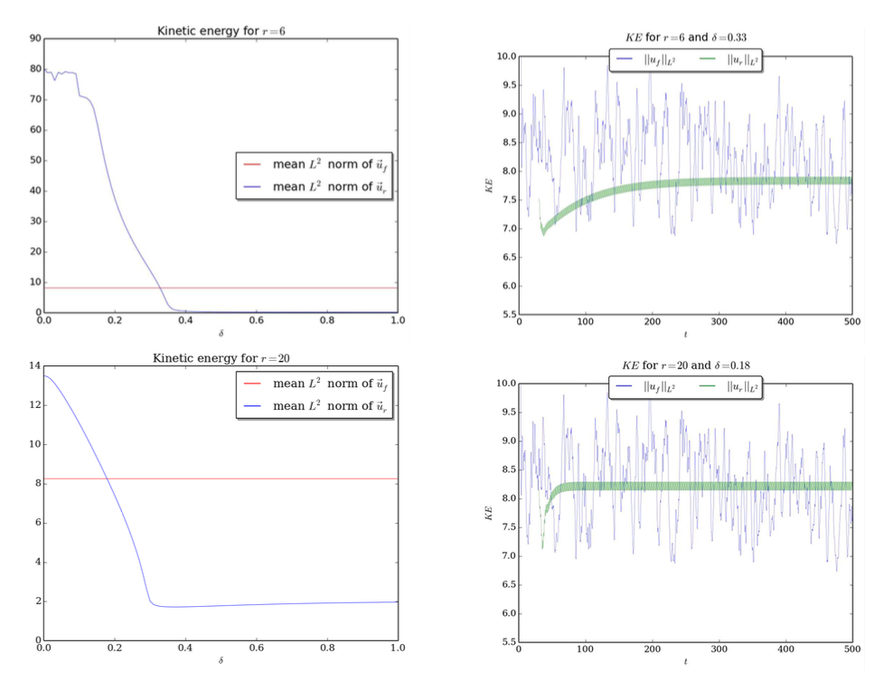
Figure 2. 3D flow past a cylinder, L-ROM (green) and DNS (blue). Mean (left column) and time evolution (right column) of the $L^{2}$ norm of the solution; $r=6$ (top row) and $r=20$ (bottom row). The time evolution of the $L^{2}$ norm of the solution (right column) is plotted for the optimal mean $L^{2}$ norm of the solution (left column): $\delta=0.33$ for $r=6$ (top row) and $\delta=0.18$ for $r=20$ (bottom row).

Fig. 3 displays the phase portraits for the first and second POD coefficients of the L-ROM-DF and POD projection of DNS data for $r=6$ and $r=20$. Fig. 3 shows that, for the optimal $\delta$ value, the L-ROM-DF yields moderately accurate results for $r=6$ and accurate results for $r=20$.

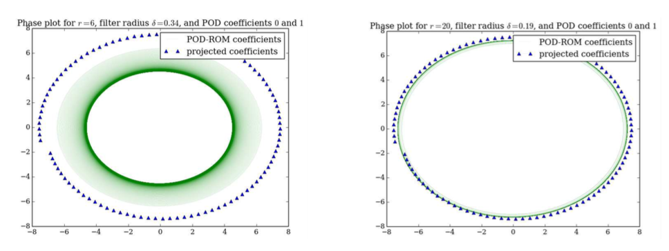
Figure 3. 3D flow past a cylinder, L-ROM-DF with optimal $\delta$ value (green) and POD projection of DNS data (blue). Phase portraits for $a_{1}$ and $a_{2}$; $r=6$ (left) and $r=20$ (right).

6. Conclusions

In this paper, we proposed a new type of ROM differential filter. We used this new filter with the L-ROM, which is one of the simplest Reg-ROMs. We tested this filter/ROM combination in the numerical simulation of a flow past a circular cylinder at Reynolds number $Re=760$ for $r=6$ and $r=20$. The new type of ROM differential filter yielded encouraging numerical results, which were comparable to those for the standard type of ROM differential filter and better than those for the ROM projection [9]. We emphasize that a major advantage of the new type of ROM differential filter over the standard ROM differential filter is its low computational overhead. Indeed, since the filtering operation in the new type of ROM differential filter is performed at a FE level (as opposed to the ROM level, as it is generally done), the new filter is applied to each ROM basis function in the offline stage. In the online stage, the computational overhead of the new type of ROM differential filter is practically zero, since it simply amounts to using the filtered ROM basis functions computed and stored in the offline stage.

The first results for the new type of ROM differential filter are encouraging. We plan to perform a thorough investigation of the new filter, including a comparison with the standard form of the ROM differential filter and the ROM projection, in the numerical simulation of realistic flows [9, 11].

References

- [1] Bangerth, W., Davydov, D., Heister, T., Heltai, L., Kanschat, G., Kronbichler, M., Maier, M., Turcksin, B, Wells, D.: The deal.ii Library, Version 8.4. J. Numer. Math. 24, 135–141 (2016)
- [2] Berselli, L.C., Iliescu, T., Layton, W.J.: Mathematics of large eddy simulation of turbulent flows, Scientific Computation. Springer-Verlag, Berlin, (2006)
- [3] Germano, M.: Differential filters of elliptic type. Phys. Fluids 29, 1757–1758 (1986)
- [4] Layton, W.J., Rebholz, L.G.: Approximate Deconvolution Models of Turbulence, vol. 2042 of Lecture Notes in Mathematics, Springer (2012)
- [5] Leray, J.: Sur le mouvement d’un liquide visqueux emplissant l’espace. Acta Math. 63, 193–248 (1934)
- [6] Sabetghadam, F., Jafarpour. A.: regularization of the POD-Galerkin dynamical systems of the Kuramoto–Sivashinsky equation. Appl. Math. Comput. 218, 6012–6026 (2012)
- [7] Sagaut, P.: Large eddy simulation for incompressible flows, Scientific Computation. Springer-Verlag, Berlin (2006)
- [8] Wang, Z., Akhtar, I., Borggaard, J.,Iliescu, T.: Proper orthogonal decomposition closure models for turbulent flows: A numerical comparison. Comput. Meth. Appl. Mech. Eng. 237-240, 10–26 (2012)
- [9] Wells, D., Wang, Z., Xie, X, Iliescu, T.: An evolve-then-filter regularized reduced order model for convection-dominated flows. Int. J. Num. Meth. Fluids to appear (2017) Available as arXiv preprint at arXiv:1506.07555 (2017).
- [10] Xie, X., Mohebujjaman, M., Rebholz, L.G., Iliescu, T.: Data-driven filtered reduced order modeling. arXiv preprint, arXiv:1702.06886 (2017)
- [11] Xie, X., Wells, D., Wang, Z., Iliescu, T.: Approximate deconvolution reduced order modeling. Comput. Methods Appl. Mech. Engrg., 313, 512–534 (2017)