Design and Optimisation of the FlyFast Front-end for Attribute-based Coordination

Abstract

Collective Adaptive Systems (CAS) consist of a large number of interacting objects. The design of such systems requires scalable analysis tools and methods, which have necessarily to rely on some form of approximation of the system’s actual behaviour. Promising techniques are those based on mean-field approximation. The FlyFast model-checker uses an on-the-fly algorithm for bounded PCTL model-checking of selected individual(s) in the context of very large populations whose global behaviour is approximated using deterministic limit mean-field techniques. Recently, a front-end for FlyFast has been proposed which provides a modelling language, PiFF in the sequel, for the Predicate-based Interaction for FlyFast. In this paper we present details of PiFF design and an approach to state-space reduction based on probabilistic bisimulation for inhomogeneous DTMCs.

1 Introduction

Collective Adaptive Systems (CAS) consist of a large number of entities with decentralised control and varying degrees of complex autonomous behaviour. They form the basis of many modern smart city critical infrastructures. Consequently, their design requires support from formal methods and scalable automatic tools based on solid mathematical foundations. In [30, 28], Latella et al. presented a scalable mean-field model-checking procedure for verifying bounded Probabilistic Computation Tree Logic (PCTL, [20]) properties of an individual in the context of a system consisting of a large number of interacting objects. The model-checking procedure is implemented in the tool FlyFast. The procedure performs on-the-fly, mean-field, approximated model-checking based on the idea of fast simulation, as introduced in [9]. More specifically, the behaviour of a generic agent with $S$ states in a system with a large number $N$ of instances of the agent at given step (i.e. time) $t$ is approximated by $\mathbf{K}(\boldsymbol{\mu}(t))$ where $\mathbf{K}({\mathbf{m}})$ is the $S\times S$ probability transition matrix of an (inhomogeneous) DTMC and $\boldsymbol{\mu}(t)$ is a vector of size $S$ approximating the mean behaviour of (the rest of) the system at $t$; each element of $\boldsymbol{\mu}(t)$ is associated with a distinct state of the agent, say $C$, and gives an approximation of the fraction of instances of the agent that are in state $C$ in the global system, at step $t$. Note that such an approximation is a deterministic one, i.e. $\boldsymbol{\mu}$ is a function of the step $t$ (the exact behaviour of the rest of the system would instead be a large DTMC in turn); note furthermore, that the above transition matrix does not depend on $N$ [30, 28].

Recently, modelling and programming languages have been proposed specifically for autonomic computing systems and CAS [13, 6]. Typically, in such frameworks, a system is composed of a set of independent components where a component is a process equipped also with a set of attributes describing features of the component. The attributes of a component can be updated during its execution so that the association between attribute names and attribute values is maintained in the dynamic store of the component. Attributes can be used in predicates appearing in language constructs for component interaction. The latter is thus typically modelled using predicate-based output/input multicast, originally proposed in [27], and playing a fundamental role in the interaction schemes of languages like SCEL [13] and Carma [6]. In fact, predicate-based communication can be used by components to dynamically organise themselves into ensembles and as a means to dynamically select partners for interaction. Furthermore, it provides a way for representing component features, like for instance component location in space, which are fundamental for systems distributed in space, such as CAS [31].

In [10] we proposed a front-end modelling language for FlyFast that provides constructs for dealing with components and predicate-based interaction; in the sequel, the language—which has been inspired by Carma— will be referred to as PiFF, which stands for for Predicate-based Interaction for FlyFast. Components interact via predicate-based communication. Each component consists of a behaviour, modelled as a DTMC-like agent, like in FlyFast, and a set of attributes. The attribute name-value correspondence is kept in the current store of the component. Actions are predicate based multi-cast output and input primitives; predicates are defined over attributes. Associated to each action there is also an (atomic) probabilistic store-update. For instance, assume components have an attribute named $\mathsf{loc}$ which takes values in the set of points of a space, thus recording the current location of the component. The following action models a multi-cast via channel $\alpha$ to all components in the same location as the sender, making it change location randomly: $\alpha^{*}[\mathsf{loc}=\mathbf{my}.\mathsf{loc}]{\langle\rangle}\mathtt{Jump}$. Here $\mathtt{Jump}$ is assumed to randomly update the store and, in particular attribute $\mathsf{loc}$. The computational model is clock-synchronous, as in FlyFast, but at the component level. In addition, each component is equipped with a local outbox. The effect of an output action $\alpha^{*}[\pi_{\_}r]{\langle\rangle}\sigma$ is to deliver output label $\alpha{\langle\rangle}$ to the local outbox, together with the predicate $\pi_{\_}r$, which (the store of) the receiver components will be required to satisfy, as well as the current store of the component executing the action; the current store is updated according to update $\sigma$. Note that output actions are non-blocking and that successive output actions of the same component overwrite its outbox. An input action $\alpha^{*}[\pi_{\_}s]()\sigma$ by a component will be executed with a probability which is proportional to the fraction of all those components whose outboxes currently contain the label $\alpha{\langle\rangle}$, a predicate $\pi_{\_}r$ which is satisfied by the component, and a store which satisfies in turn predicate $\pi_{\_}s$. If such a fraction is zero, then the input action will not take place (input is blocking), otherwise the action takes place, the store of the component is updated via $\sigma$, and its outbox cleared.

Related Work

CAS are typically large systems, so that the formal analysis of models for such systems hits invariantly the state-space explosion problem. In order to mitigate this problem, the so called ‘on-the-fly’ paradigm is often adopted (see e.g. [11, 5, 22, 17]).

In the context of probabilistic model-checking several on-the-fly approaches have been proposed, among which [14], [29] and [19]. In [14], a probabilistic model-checker is shown for the time bounded fragment of PCTL. An on-the-fly approach for full PCTL model-checking is proposed in [29] where, actually, a specific instantiation is presented of an algorithm which is parametric with respect to the specific probabilistic processes modelling language and logic, and their specific semantics. Finally, in [19] an on-the-fly approach is used for detecting a maximal relevant search depth in an infinite state space and then a global model-checking approach is used for verifying bounded Continuous Stochastic Logic (CSL) [2, 3] formulas in a continuous time setting on the selected subset of states.

An on-the-fly approach by itself however, does not solve the challenging scalability problems that arise in truly large parallel systems, such as CAS. To address this type of scalability challenges in probabilistic model-checking, recently, several approaches have been proposed. In [21, 18] approximate probabilistic model-checking is introduced. This is a form of statistical model-checking that consists in the generation of random executions of an a priori established maximal length [26]. On each execution the property of interest is checked and statistics are performed over the outcomes. The number of executions required for a reliable result depends on the maximal error-margin of interest. The approach relies on the analysis of individual execution traces rather than a full state space exploration and is therefore memory-efficient. However, the number of execution traces that may be required to reach a desired accuracy may be large and therefore time-consuming. The approach works for general models, i.e. models where stochastic behaviour can also be non Markovian and that do not necessarily model populations of similar objects. On the other hand, the approach is not independent from the number of objects involved. As recalled above, in [28] a scalable model-checking algorithm is presented that is based on mean-field approximation, for the verification of time bounded PCTL properties of an individual in the context of a system consisting of a large number of interacting objects. Correctness of the algorithm with respect to exact probabilistic model-checking has been proven in [28] as well. Also this algorithm is actually an instantiation of the above mentioned parametric algorithm for (exact) probabilistic model-checking [29], but the algorithm is instantiated on (time bounded PCTL and) the approximate, mean-field, semantics of a population process modelling language. It is worth pointing out that FlyFast allows users to perform simulations of their system models and to analyse the latter using their exact probabilistic semantics and exact PCTL model-checking. In addition, the tool provides approximate model-checking for bounded PCTL, using the model semantics based on mean-field.

The work of Latella et al. [28] is based on mean-field approximation in the discrete time setting; approximated mean-field model-checking in the continuous time setting has been presented in the literature as well, where the deterministic approximation of the global system behaviour is formalised as an initial value problem using a set of differential equations. Preliminary ideas on the exploitation of mean-field convergence in continuous time for model-checking were informally sketched in [24], but no model-checking algorithms were presented. Follow-up work on the above mentioned approach can be found in [25] which relies on earlier results on fluid model-checking by Bortolussi and Hillston [7], later published in [8], where a global CSL model-checking procedure is proposed for the verification of properties of a selection of individuals in a population, which relies on fast simulation results. This work is perhaps closest related to [28, 30]; however their procedure exploits mean-field convergence and fast simulation [12, 16] in a continuous time setting—using a set of differential equations—rather than in a discrete time setting—where an inductive definition is used. Moreover, that approach is based on an interleaving model of computation, rather than a clock-synchronous one; furthermore, a global model-checking approach, rather than an on-the-fly approach is adopted; it is also worth noting that the treatment of nested formulas, whose truth value may change over time, turns out to be much more difficult in the interleaving, continuous time, global model-checking approach than in the clock-synchronous, discrete time, on-the-fly one.

PiFF has been originally proposed in [10], where the complete formal, exact probabilistic, semantics of the language have been defined. The semantics definition consists of three transition rules—one for transitions associated with output actions, one for those associated with input actions, and one for transitions to be fired with residual probability. The rules induce a transition relation among component states and compute the relevant probabilities. From the component transition relation, a component one-step transition probability matrix is derived, the elements of which may depend on the fractions of the components in the system which are in a certain state. The system-wide one-step transition probability matrix is obtained by product—due to independence assumptions—using the above mentioned component probability matrix and the actual fractions in the current system global state. In [10] a translation of PiFF to the model specification language of FlyFast has also been presented which makes PiFF an additional front-end for FlyFast extending its applicability to models of systems based on predicate-based interaction. In the above mentioned paper, correctness of the translation has been proved as well. In particular, it has been shown that the probabilistic semantics of any PiFF model are isomorphic to those of the translation of the model. In other words, the transition probability matrix of (the DTMCs of) the two models is the same. A companion translation of bounded PCTL formulas is also defined [10] and proven correct.

The notion of the outbox used in PiFF is reminiscent of the notion of the ether in PALOMA [15] in the sense that the collection of all outboxes together can be thought of as a kind of ether; but such a collection is intrinsically distributed among the components so that it cannot represent a bottleneck in the execution of the system neither a singularity point in the deterministic approximation.

We are not aware of other proposals, apart from [10], of probabilistic process languages, equipped both with standard, DTMC-based, semantics and with mean-field ones, that provide a predicate-based interaction framework, and that are fully supported by a tool for probabilistic simulation, exact and mean-field model-checking.

We conclude this section recalling that mean-field/fluid procedures are based on approximations of the global behaviour of a system. Consequently, the techniques should be considered as complementary to other, possibly more accurate but often not as scalable, analysis techniques for CAS, primarily those based on stochastic simulation, such as statistical model-checking.

In this paper we present some details of PiFF, a translation to FlyFast which simplifies that proposed in [10] and an approach to model reduction based on probabilistic bisimulation for Inhomogeneous DTMCs. In Section 2 we briefly present the main ingredients of the PiFF syntax and informal semantics, and we recall those features of FlyFast directly relevant for understanding the translation of PiFF to the FlyFast input language proposed in [10]. A revised and simplified version of the translation is described in Section 3. In Section 4 we introduce a simplified language for the definition of transition-probabilities in PiFF that allows us to define in Section 5 a model reduction procedure of the translation result, based on a notion of bisimulation for the kind of IDTMCs of interest, introduced in Section 5 as well. An example of application of the procedure is presented in Section 6. Some conclusions are drawn in Section 7. A formal proof of decidability of the cumulative probability test for state-space reduction based on bisimulation is provided in the Appendix.

2 Summary on PiFF and FlyFast

In the following we present the main ingredients of PiFF and the features of FlyFast relevant for the present paper.

2.1 PiFF

A PiFF system model specification $\Upsilon=(\Delta_{\_}{\Upsilon},F_{\_}{\Upsilon},\boldsymbol{\Sigma_{\_}0})^{(N)}$ is a triple where $F_{\_}{\Upsilon}$ is the set of relevant function definitions (e.g. store updates, auxiliary constants and functions), $\Delta_{\_}{\Upsilon}$ is a set of state defining equations, and $\boldsymbol{\Sigma_{\_}0}$ is the initial system state (an $N$-tuple of component states, each of which being a 3-tuple $(C,\gamma,O)$ of agent state $C$, store $\gamma$ and outbox $O$). We describe the relevant details below referring to [10] for the formal definition probabilistic semantics of the language.

The PiFF type system consists of floating point values and operations, as in FlyFast, plus simple enumeration types for attributes, declared according to the syntax $\mathbf{attype}\;\mathtt{<name>}\;\mathbf{enum}\;\mathtt{<id-list>}$. $\mathtt{<id-list>}$ is a finite list of identifiers. Of course, attributes can also take floating point values.

$\mathbf{attype}\;\mathtt{Space}\;\mathbf{enum}\;\mathtt{A,B,C,D};\\ \vdots\\ \mathbf{const}\;\mathtt{H}=0.6;\\ \mathbf{const}\;\mathtt{L=1-H};\\ \mathbf{const}\;\mathtt{Hdiv2=H/2};\\ \mathbf{const}\;\mathtt{Ldiv2=L/2};\\ \vdots\\ \mathbf{attribute}\;\mathsf{loc}:\mathtt{Space};\\ \vdots\\ \mathbf{func}\;\mathtt{Hr}(x:\mathtt{Space}):\mathtt{Space};\;x\;\mathbf{endfunc};\\ \mathbf{func}\;\mathtt{N}(x:\mathtt{Space}):\mathtt{Space};\;\mathbf{case}\;x\;\mathbf{of}\;\mathtt{A:A;B:B;C:B;D:A}\;\mathbf{endfunc};\\ \mathbf{func}\;\mathtt{S}(x:\mathtt{Space}):\mathtt{Space};\;\mathbf{case}\;x\;\mathbf{of}\;\mathtt{A:D;B:C;C:C;D:D}\;\mathbf{endfunc};\\ \mathbf{func}\;\mathtt{E}(x:\mathtt{Space}):\mathtt{Space};\;\mathbf{case}\;x\;\mathbf{of}\;\mathtt{A:A;B:A;C:D;D:D}\;\mathbf{endfunc};\\ \mathbf{func}\;\mathtt{W}(x:\mathtt{Space}):\mathtt{Space};\;\mathbf{case}\;x\;\mathbf{of}\;\mathtt{A:B;B:B;C:C;D:C}\;\mathbf{endfunc};\\ \vdots\\ \mathbf{func}\;\mathtt{pHr}(x:\mathtt{Space}):\mathbf{float};\;\mathbf{case}\;x\;\mathbf{of}\;\mathtt{A:H;B:L;C:H;D:L}\;\mathbf{endfunc};\\ \mathbf{func}\;\mathtt{pN}(x:\mathtt{Space}):\mathbf{float};\;\mathbf{case}\;x\;\mathbf{of}\;\mathtt{A:0;B:0;C:Ldiv2;D:Hdiv2}\;\mathbf{endfunc};\\ \mathbf{func}\;\mathtt{pS}(x:\mathtt{Space}):\mathbf{float};\;\mathbf{case}\;x\;\mathbf{of}\;\mathtt{A:Ldiv2;B:Hdiv2;C:0;D:0}\;\mathbf{endfunc};\\ \mathbf{func}\;\mathtt{pE}(x:\mathtt{Space}):\mathbf{float};\;\mathbf{case}\;x\;\mathbf{of}\;\mathtt{A:0;B:Hdiv2;C:Ldiv2;D:0}\;\mathbf{endfunc};\\ \mathbf{func}\;\mathtt{pW}(x:\mathtt{Space}):\mathbf{float};\;\mathbf{case}\;x\;\mathbf{of}\;\mathtt{A:Ldiv2;B:0;C:0;D:Hdiv2}\;\mathbf{endfunc};\\ \vdots\\ \mathbf{update}\;\mathtt{Jump}\\ \mathbf{my}.\mathsf{loc}:=\mathtt{Hr}(\mathbf{my}.\mathsf{loc})\;\mathbf{with}\;\mathtt{pHr}(\mathbf{my}.\mathsf{loc});\\ \mathbf{my}.\mathsf{loc}:=\mathtt{N}(\mathbf{my}.\mathsf{loc})\;\mathbf{with}\;\mathtt{pN}(\mathbf{my}.\mathsf{loc});\\ \mathbf{my}.\mathsf{loc}:=\mathtt{S}(\mathbf{my}.\mathsf{loc})\;\mathbf{with}\;\mathtt{pS}(\mathbf{my}.\mathsf{loc});\\ \mathbf{my}.\mathsf{loc}:=\mathtt{E}(\mathbf{my}.\mathsf{loc})\;\mathbf{with}\;\mathtt{pE}(\mathbf{my}.\mathsf{loc});\\ \mathbf{my}.\mathsf{loc}:=\mathtt{W}(\mathbf{my}.\mathsf{loc})\;\mathbf{with}\;\mathtt{pW}(\mathbf{my}.\mathsf{loc})\\ \mathbf{endupdate}$

Figure 1: A fragment of $F_{\_}{SI}$.

In Figure 1 the attribute type $\mathtt{Space}$ is defined that consists of four values $\mathtt{A,B,C,D}$ modelling four locations. Some auxiliary constants are defined, using the $\mathbf{const}$ construct inherited from FlyFast: $\mathbf{const}\;\mathtt{<name>}\,=\,\mathtt{<value>}$.

A PiFF store update definition has the following syntax:

$\mathbf{update}{}\;upd\\ \mathbf{my}.a_{\_}1:=e_{\_}{11},\ldots,\mathbf{my}.a_{\_}k:=e_{\_}{k1}\mathbf{with}{}\;p_{\_}1;\\ \vdots\\ \mathbf{my}.a_{\_}1:=e_{\_}{1n},\ldots,\mathbf{my}.a_{\_}k:=e_{\_}{kn}\mathbf{with}{}\;p_{\_}n\\ \mathbf{endupdate}$

where $upd$ is the update name (unique within the system model specification), $a_{\_}1,\ldots,a_{\_}k$ are the attribute names of the component, $e_{\_}{11},\ldots,e_{\_}{kn}$ and $p_{\_}1,\ldots,p_{\_}n$ are attribute/store-probability expressions respectively, with syntax defined according to the grammars $e::=v_{\_}a\;|\;c_{\_}a\;|\;\mathbf{my}.a\;|\;fn_{\_}a(e_{\_}1,\ldots,e_{\_}m)$ and $p::=v_{\_}p\;|\;c_{\_}p\;|\;fn_{\_}p(e_{\_}1,\ldots,e_{\_}m).$ In the above definition of attribute expressions $v_{\_}a$ is an attribute value (drawn from finite set ${\cal V}$ of attribute values), $c_{\_}a$ is an attribute constant in ${\cal V}$ defined using the $\mathbf{const}$; $a\in\{a_{\_}1,\ldots,a_{\_}k\}$ is an attribute name and $fn_{\_}a$ is an attribute function defined by the user in $F_{\_}{\Upsilon}$, which, when applied to attribute expressions $e_{\_}1,\ldots,e_{\_}m$ returns an attribute value; the syntax for such function definitions $\mathit{afd}$ is given below:

$\mathit{afd}::=\mathbf{func}\;fn_{\_}a(x_{\_}1:T1,\ldots,x_{\_}m:Tm):T;\mathit{afb}\;\mathbf{endfunc}\\$ $\mathit{afb}::=e\;|\mathbf{case}\;(x_{\_}1,\ldots,x_{\_}m)\;\mathbf{of}(v_{\_}{a_{\_}{11}},\ldots,v_{\_}{a_{\_}{m1}}):e_{\_}{1};(v_{\_}{a_{\_}{12}},\ldots,v_{\_}{a_{\_}{m2}}):e_{\_}{2};\ldots(v_{\_}{a_{\_}{1k}},\ldots,v_{\_}{a_{\_}{mk}}):e_{\_}{k}$

where $fn_{\_}a$ is the name of the attribute function, $x_{\_}1:T1,\ldots,x_{\_}m:Tm$ are its parameters and their relative types, $T$ is the type of the result of $fn_{\_}a$; $e$, $e_{\_}{i}$ are attribute-expressions and $v_{\_}{a_{\_}{ij}}$ are attribute-values.

In Figure 1 attribute functions $\mathtt{N,S,E,W}$ are defined for North, South, East, and West, such that $\mathtt{Space}$ models the Cartesian space with four quadrants: $\mathtt{A=N(D)=E(B)}$, $\mathtt{B=N(C)=W(A)}$, and so on, as shown diagrammatically in Figure 2 right. Function $\mathtt{Hr}$ is the identity on $\mathtt{Space}$.

In the definition of store-probability expressions $v_{\_}p\in(0,1]$, $c_{\_}p$ is a store-probability constant in $(0,1]$ defined using the FlyFast $\mathbf{const}$ construct, and $fn_{\_}p$ is a store-probability function defined by the user in $F_{\_}{\Upsilon}$, which, when applied to attribute expressions $e_{\_}1,\ldots,e_{\_}m$ returns a probability value.The syntax for store-probability function definitions $\mathit{pfd}$ is similar to that of attribute functions:

$\mathit{pfd}::=\mathbf{func}\;fn_{\_}p(x_{\_}1:T1,\ldots,x_{\_}m:Tm):\mathbf{float};\mathit{pfb}\;\mathbf{endfunc}\\$ $\mathit{pfb}::=p\;|\mathbf{case}\;(x_{\_}1,\ldots,x_{\_}m)\;\mathbf{of}(v_{\_}{a_{\_}{11}},\ldots,v_{\_}{a_{\_}{m1}}):p_{\_}{1};(v_{\_}{a_{\_}{12}},\ldots,v_{\_}{a_{\_}{m2}}):p_{\_}{2};\ldots(v_{\_}{a_{\_}{1k}},\ldots,v_{\_}{a_{\_}{mk}}):p_{\_}{k}$

where $fn_{\_}p$ is the name of the store-probability function, the result type is $\mathbf{float}$ (actually the range $[0,1]$) $x_{\_}1:T1,\ldots,x_{\_}m:Tm$ are its parameters and their relative types, $p$, $p_{\_}{i}$ are store-probability expressions and $v_{\_}{a_{\_}{ij}}$ are attribute-values. In any store update definition it must be guaranteed that the values of $p_{\_}1\ldots p_{\_}n$ sum up to $1$. The informal meaning is clear. The store update will make attributes $a_{\_}1,\ldots,a_{\_}k$ take the values of $e_{\_}{1i},\ldots,e_{\_}{ki}$ respectively with probability equal to the value of $p_{\_}i$.

In Figure 1 store-probability functions $\mathtt{pHr,pN,pS,pE,pW}$ are defined that give the probabilities of not moving ($\mathtt{pHr}$), or of jumping to North ($\mathtt{pN}$), South ($\mathtt{pS}$), East ($\mathtt{pE}$), West ($\mathtt{pW}$), as functions of the current location.

Example 1

A simplified version of the behaviour of the epidemic process discussed in [10] is shown in Figure 2 left. In Figure 1 we show a fragment of $F_{\_}{SI}$ defining store update $\mathtt{Jump}$ together with the relevant type, constant and function definitions as introduced above. The component has just one attribute, named $\mathsf{loc}$, with values in $\mathtt{Space}$. The effect of $\mathtt{Jump}$ executed by a component in which $\mathsf{loc}$ is bound to quadrant $\ell$ is to leave the value of $\mathsf{loc}$ unchanged with probability $\mathtt{pHr}(\ell)$, change it to the quadrant North of $\ell$ with probability $\mathtt{pN}(\ell)$, and so on. Note that $\mathtt{H}>\mathtt{L}$ and this implies that higher probability is assigned to $\mathtt{A}$ and $\mathtt{C}$ and low probability to $\mathtt{B}$ and $\mathtt{D}$. This is represented in Figure 2 right where higher probability locations are shown in green and lower probability ones are shown in red; moreover, the relevant probabilities are represented as arrows ($\mathtt{H/2},\mathtt{L/2}$) or self-loops ($\mathtt{H},\mathtt{L}$). A susceptible (state $\mathtt{S}$) component becomes infected (state $\mathtt{I}$) via an $\mathtt{inf}$ action which takes place with probability equal to the fraction of components in the system which are currently infected (i.e. $\mathtt{frc(I)}$); it remains in state $\mathtt{S}$ via the self-loop labelled by action $\mathtt{nsc}$, with probability $\mathtt{frc(S)=1-frc(I)}$. An infected node (state $\mathtt{I}$) may recover, entering state $\mathtt{S}$ with action $\mathtt{rec}$ and probability $\mathtt{ir}$; while infected, it keeps executing action $\mathtt{inf}$, with probability $\mathtt{ii}$. Note that, for the sake of simplicity, we use only internal actions, modelled by means of output actions with predicate false ($\bot$). We assume that in the initial global state all outboxes are non-empty; each contains the initial store of the specific component (i.e., its initial location), predicate $\bot$ and the empty tuple ${\langle\rangle}$).

$\begin{array}[]{l l l }\texttt{S}&:=&\textsf{frc}\,(\texttt{I})::\texttt{inf}^{*}[\bot]{\langle\rangle}\texttt{Jump}.\texttt{I +}\\ &&\textsf{frc}\,(\texttt{S})::\texttt{nsc}^{*}[\bot]{\langle\rangle}\texttt{Jump}.\texttt{S}\\ \\ \texttt{I}&:=&ii::\texttt{inf}^{*}[\bot]{\langle\rangle}\texttt{Jump}.\texttt{I +}\\ &&ir::\texttt{rec}^{*}[\bot]{\langle\rangle}\texttt{Jump}.\texttt{S}\\ \\ \\ \\ \\ \\ \\ \\ \end{array}$

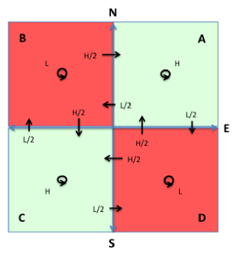
Figure 2: $SI$, a behavioural model.

A PiFF state defining equation has the following (abstract) form: $C:=\sum_{\_}{j\in J}[g_{\_}j]p_{\_}j::act_{\_}j.C_{\_}j$ where either $[g_{\_}j]p_{\_}j$ is the keyword $\mathbf{rest}$ or:

• $g_{\_}j$ is a boolean expression $b$ which may depend on the current store, but not on the current occupancy measure vector: $b::=\top\;|\;\bot\;|\;e\,\underline{\bowtie}\,e\;|\;\neg b\;|\;b\and b$ and $e::=v_{\_}a\;|\;c_{\_}a\;|\mathbf{my}.a$ where $\top$ ($\bot$) denotes the constant $\mathtt{true}$ ($\mathtt{false}$), $\underline{\bowtie}\,\in\{\geq,>,\leq,<\}$, $v_{\_}a$ is an attribute value (drawn from finite set ${\cal V}$ of attribute values), $c_{\_}a$ is an attribute constant in ${\cal V}$ defined using the FlyFast $\mathbf{const}$ construct, and $a$ is the name of an attribute of the component.

• $p_{\_}j$ is a transition probability expression $p::=v_{\_}p\,|\,c_{\_}p\,|\,\textsf{frc}\,(C)\,|\,\textsf{frc}\,(\pi)\,|\,\prod_{\_}{i\in I}\;p_{\_}i\,|\,\sum_{\_}{i\in I}p_{\_}i\,|\,1-p$, for finite $I$, where $v_{\_}p\in(0,1]$, $c_{\_}p$ a constant in $(0,1]$ defined via the $\mathbf{const}$ construct, and $\pi$ is defined as $b$ above, but where expressions $e$ can also be attribute names $a$ (i.e. $e::=v_{\_}a\;|\;c_{\_}a\;|\;\mathbf{my}.a\;|\;a$); $\textsf{frc}\,(C)$ is the fraction of components currently in state $C$ over the total number $N$; similarly, $\textsf{frc}\,(\pi)$ is the fraction of components the current store of which satisfies $\pi$, over the total number $N$. Note that it must be guaranteed that $\prod_{\_}{i\in I}p_{\_}i\leq 1$ and $\sum_{\_}{i\in I}p_{\_}i\leq 1$.

• $act_{\_}j$ can be an output action $\alpha^{*}[\pi]{\langle\rangle}\sigma$ or an input action $\alpha^{*}[\pi]()\sigma$, where $\pi$ is as above and $\sigma$ is the name of a store update. Note that in the case of an input action, $\pi$ refers to the store of the partner component in the previous step of the computation.

If $[g_{\_}j]p_{\_}j=\mathbf{rest}$, then $act_{\_}j$ must be an output action $\alpha^{*}[\pi]{\langle\rangle}\sigma$, to be executed with the residual probability.

2.2 FlyFast

FlyFast accepts a specification ${\langle\Delta,A,{\mathbf{C}_{\_}0}\rangle}^{(N)}$ of a model of a system consisting of the clock-synchronous product of $N$ instances of a probabilistic agent. The states of the DTMC-like agent model are specified by a set of state-defining equations $\Delta$. The (abstract) form of a state defining equation is the following $C:=\sum_{\_}{i=1}^{r}a_{\_}i.C_{\_}i$ where $a_{\_}i\in{{\cal A}}$—the set of FlyFast actions—$C,C_{\_}i\in{\cal S}$—the set of FlyFast states—and, for $i,j=1,\ldots,r$ $a_{\_}i\not=a_{\_}j$ if $i\not=j$; note that $C_{\_}i=C_{\_}j$ with $i\not=j$ is allowed instead. Each action has a probability assigned by means of an action probability function definition in $A$ of the form $a::exp$ where $exp$ is an expression consisting of constants and $\textsf{frc}\,(C)$ terms. Constants are floating point values or names associated to such values using the construct $\mathbf{const}\;\mathtt{<name>}\,=\,\mathtt{<value>}$; $\textsf{frc}\,(C)$ denotes the element associated to state $C$ in the current occupancy measure vector. So, strictly speaking, $\Delta$ and $A$ characterise an inhomogeneous DTMC whose probability matrix $\mathbf{K}({\mathbf{m}})$ is a function of the occupancy measure vector ${\mathbf{m}}$ such that for each pair of states $C,C^{\prime}$, the matrix element $\mathbf{K}({\mathbf{m}})_{\_}{C,C^{\prime}}$ is the probability of jumping from $C$ to $C^{\prime}$ given the current occupancy measure vector ${\mathbf{m}}$. Letting ${\cal S}_{\Delta}$ be the set of states of the agent, with $|{\cal S}_{\Delta}|=S$, and ${\cal U}^{S}=\{(m_{\_}1,\ldots,m_{\_}S)|m_{\_}1+\ldots+m_{\_}S=1\}$ denote the unit simplex of dimension $S$, we have $\mathbf{K}:{\cal U}^{S}\times{\cal S}_{\Delta}\times{\cal S}_{\Delta}\rightarrow[0,1]$. Matrix $\mathbf{K}$ is generated directly from the input specification ${\langle\Delta,A,{\mathbf{C}_{\_}0}\rangle}^{(N)}$; the reader interested in the details of how to derive $\mathbf{K}$ is referred to [28, 30]. Auxiliary function definitions can be specified in $A$. The initial state ${\mathbf{C}_{\_}0}$ is a vector of size $N$ consisting of the initial state of each individual object. Finally, note that in matrix $\mathbf{K}({\mathbf{m}})$ the information on specific actions is lost, which is common in PCTL/DTMC based approaches; furthermore, we note that, by construction, $\mathbf{K}({\mathbf{m}})$ does not depend on $N$ (see [28, 30] for details).

3 A revised translation

As in [10], we define a translation such that, given a PiFF system specification $\Upsilon=(\Delta_{\_}{\Upsilon},F_{\_}{\Upsilon},\boldsymbol{\Sigma_{\_}0})^{(N)}$, the translation returns the FlyFast system specification ${\langle\Delta,A,{\mathbf{C}_{\_}0}\rangle}^{(N)}$ preserving probabilistic semantics. The predicate-based FlyFast front-end is then completed with a simple translation at the PCTL level, for which we refer to [10].

The system model specification translation consists of two phases. In the first phase, each action in the input system model specification $\Upsilon$ is annotated with an identifier which is unique within the specification. We let $\aleph(\Upsilon)$ denote the resulting specification. These annotations will make action names unique specification-wide thus eliminating complications which may arise from multiple occurrences of the same action, in particular when leading to the same state (see [10] for details). Of course, these annotations are disregarded in the probabilistic semantics, when considering the interaction model of components. In other words, an output action $\alpha{\langle\rangle}$ in outbox $(\gamma,\pi,\alpha{\langle\rangle})$ must match with any input action $\alpha()$ even if $\alpha{\langle\rangle}$ would actually correspond to $(\alpha,\iota)^{*}[\pi]{\langle\rangle}$ and $\alpha()$ would actually correspond to $(\alpha,\eta)^{*}[\pi^{\prime}]()$. Apart from this detail, the probabilistic semantics as defined in [10] remain unchanged.

The second phase is defined by the translation algorithm defined in Figure 5, which is a revised and simplified version of that presented in [10] and is applied to $\aleph(\Upsilon)$. We let ${\cal I}(\aleph(\Upsilon))$ denote the result of the translation, namely the pure FlyFast system specification ${\langle\Delta,A,{\mathbf{C}_{\_}0}\rangle}^{(N)}$.

We recall here some notation from [10]. We let ${\cal S}_{\Delta_{\_}{\Upsilon}}$ denote the set of states of $\Upsilon$; $\Gamma_{\_}{\Delta_{\_}{\Upsilon}}$ is the set of all stores defined over the attributes of $\Upsilon$—a store is a finite mapping from the attributes of the component to a finite set of values ${\cal V}$, thus $\Gamma_{\_}{\Delta_{\_}{\Upsilon}}$ is finite—and ${\cal O}_{\_}{\Delta_{\_}{\Upsilon}}$ the finite set of all outboxes of $\Upsilon$. A $\Upsilon$ component-state is a triple $(C,\gamma,O)\in{\cal S}_{\Delta_{\_}{\Upsilon}}\times\Gamma_{\_}{\Delta_{\_}{\Upsilon}}\times{\cal O}_{\_}{\Delta_{\_}{\Upsilon}}=\Omega_{\_}{\Delta_{\_}{\Upsilon}}$. If the component-state is the target of a transition modelling the execution of an output action, then $O=(\gamma^{\prime},\pi,\alpha{\langle\rangle})$, where $\gamma^{\prime}$ is the store of the (component-state) source of the transition, $\pi$ is the predicate used in the action—actualised with $\gamma^{\prime}$—and $\alpha{\langle\rangle}$ the actual message sent by the action. If, instead, the component-state is the target of a transition for an input action, then $O={\langle\rangle}$, i.e. the empty outbox. Note that the set of component states of $\aleph(\Upsilon)$ is identical to that of $\Upsilon$. Also the set of all stores of $\aleph(\Upsilon)$ is the same as that of $\Upsilon$. In the algorithm of Figure 5 by $t*t^{\prime}$ we mean the syntactical term representing the product of terms $t$ and $t^{\prime}$; the notation is extended to $\mathsf{PROD}\{t|\mathsf{cond}(t)\}$, denoting the syntactical product $t_{\_}1*\ldots*t_{\_}n$ if $\{t|\mathsf{cond}(t)=\mbox{tt}\}=\{t_{\_}1,\ldots,t_{\_}n\}\not=\emptyset$ and $1$ otherwise. Similarly, $\mathsf{SUM}\{t|\mathsf{cond}(t)\}$ denotes the syntactical sum $t_{\_}1+\ldots+t_{\_}n$ if $\{t|\mathsf{cond}(t)=\mbox{tt}\}=\{t_{\_}1,\ldots,t_{\_}n\}\not=\emptyset$ and $0$ otherwise. The translation algorithm uses a few auxiliary functions which we briefly discuss below:

• ${\cal I}_{\_}{{\cal S}}:\Omega_{\_}{\Delta_{\_}{\Upsilon}}\rightarrow{\cal S}$ is a total injection which maps every component state of $\aleph(\Upsilon)$ to a distinct state of ${\cal I}(\aleph(\Upsilon))$; we recall that ${\cal S}$ denotes the set of state names of FlyFast models.

• ${\cal I}_{\_}{{{\cal A}}}:({\cal S}_{\Delta_{\_}{\Upsilon}}\times\Gamma_{\_}{\Delta_{\_}{\Upsilon}})\times(\Lambda_{\_}{\Delta_{\_}{\Upsilon}}\times I_{\_}{\aleph})\times\Omega_{\_}{\Delta_{\_}{\Upsilon}}\rightarrow{{\cal A}}$ is a total injection where, as in [10], $\Lambda_{\_}{\Delta_{\_}{\Upsilon}}$ is the set of action labels of $\Upsilon$ and $I_{\_}{\aleph}$ is the set of unique identifiers used in the first phase of the translation. We recall that ${{\cal A}}$ is the set of action names of FlyFast. The mapping of actions is a bit more delicate because we have to respect FlyFast static constraints and, in particular, we have to avoid multiple probability function definitions for the same action. A first source of potential violations (i.e. multiple syntactical occurrences of the same action) has been removed by action annotation in the first phase of the translation. A second source is the fact that the same action can take place in different contexts (for example with different stores) or leading to different target component states (maybe with different probabilities). To that purpose, we could distinguish different occurrences of the same action in different transitions, each characterised by its source component-state and its target component-state in $\Omega_{\_}{\Delta_{\_}{\Upsilon}}$. In practice, since an action of a component cannot be influenced by the current outbox of the component, it is sufficient to restrict the first component of the domain from $\Omega_{\_}{\Delta_{\_}{\Upsilon}}$ to $({\cal S}_{\Delta_{\_}{\Upsilon}}\times\Gamma_{\_}{\Delta_{\_}{\Upsilon}})$.

• The interpretation functions defined in Figure 3, namely those depending on stores only (and not on occupancy measure vectors); we assume $\mathbf{E_{\_}L}[\![\cdot]\!]_{\_}{\gamma}$ extended to $\mathbf{E_{\_}L}[\![fn]\!]_{\_}{\gamma}$ for defined function $fn$, in the standard way. In Figure 3 $\beta_{\_}{\Upsilon}$ denotes the constant to value bindings generated by the $\mathbf{const}$ construct in the input model specification $\Upsilon$, whereas store update $upd$ is defined as above.

• The translation function ${\cal I}_{\_}{{\cal P}}$ for transition probability expressions $p_{\_}j$, defined in Figure 4.

$\begin{array}[]{l c l}\mathbf{E_{\_}L}[\![\top]\!]_{\_}{\gamma}&=&\mbox{tt}\\ \mathbf{E_{\_}L}[\![\bot]\!]_{\_}{\gamma}&=&\mbox{ff}\\ \mathbf{E_{\_}L}[\![e_{\_}1\,\underline{\bowtie}\,e_{\_}2]\!]_{\_}{\gamma}&=&\mathbf{E_{\_}L}[\![e_{\_}1]\!]_{\_}{\gamma}\,\underline{\bowtie}\,\mathbf{E_{\_}L}[\![e_{\_}2]\!]_{\_}{\gamma}\\ \mathbf{E_{\_}L}[\![\neg b]\!]_{\_}{\gamma}&=&\neg\mathbf{E_{\_}L}[\![b]\!]_{\_}{\gamma}\\ \mathbf{E_{\_}L}[\![b_{\_}1\and b_{\_}2]\!]_{\_}{\gamma}&=&\mathbf{E_{\_}L}[\![b_{\_}1]\!]_{\_}{\gamma}\and\mathbf{E_{\_}L}[\![b_{\_}2]\!]_{\_}{\gamma}\\ \mathbf{E_{\_}L}[\![v_{\_}a]\!]_{\_}{\gamma}&=&v_{\_}a\\ \mathbf{E_{\_}L}[\![c_{\_}a]\!]_{\_}{\gamma}&=&\beta_{\_}{\Upsilon}(c_{\_}a)\\ \mathbf{E_{\_}L}[\![v_{\_}p]\!]_{\_}{\gamma}&=&v_{\_}p\\ \mathbf{E_{\_}L}[\![c_{\_}p]\!]_{\_}{\gamma}&=&\beta_{\_}{\Upsilon}(c_{\_}p)\\ \mathbf{E_{\_}L}[\![a]\!]_{\_}{\gamma}&=&a\\ \mathbf{E_{\_}L}[\![\mathbf{my}.a]\!]_{\_}{\gamma}&=&\gamma(a)\end{array}$
$\begin{array}[]{l c l}\mathbf{E_{\_}L}[\![fn_{\_}a(e_{\_}1,\ldots,e_{\_}m)]\!]_{\_}{\gamma}&=&\mathbf{E_{\_}L}[\![fn_{\_}a]\!]_{\_}{\gamma}(\mathbf{E_{\_}L}[\![e_{\_}1]\!]_{\_}{\gamma},\ldots,\mathbf{E_{\_}L}[\![e_{\_}m]\!]_{\_}{\gamma})\\ \mathbf{E_{\_}L}[\![fn_{\_}p(e_{\_}1,\ldots,e_{\_}m)]\!]_{\_}{\gamma}&=&\mathbf{E_{\_}L}[\![fn_{\_}p]\!]_{\_}{\gamma}(\mathbf{E_{\_}L}[\![e_{\_}1]\!]_{\_}{\gamma},\ldots,\mathbf{E_{\_}L}[\![e_{\_}m]\!]_{\_}{\gamma})\end{array}$

$\begin{array}[]{l c l}\mathbf{E_{\_}U}[\![upd]\!]_{\_}{\gamma}&=&\lambda\gamma^{\prime}.\mathtt{dom}(\gamma^{\prime})\not=\{a_{\_}1,\ldots,a_{\_}k\}\rightarrow 0;\\ &&\hskip 15.89948pt\gamma^{\prime}(a_{\_}1)=\mathbf{E_{\_}L}[\![e_{\_}{11}]\!]_{\_}{\gamma}\and\ldots\and\gamma^{\prime}(a_{\_}k)=\mathbf{E_{\_}L}[\![e_{\_}{k1}]\!]_{\_}{\gamma}\rightarrow\mathbf{E_{\_}L}[\![p_{\_}1]\!]_{\_}{\gamma};\\ &&\hskip 15.89948pt\vdots\\ &&\hskip 15.89948pt\gamma^{\prime}(a_{\_}1)=\mathbf{E_{\_}L}[\![e_{\_}{1n}]\!]_{\_}{\gamma}\and\ldots\and\gamma^{\prime}(a_{\_}k)=\mathbf{E_{\_}L}[\![e_{\_}{kn}]\!]_{\_}{\gamma}\rightarrow\mathbf{E_{\_}L}[\![p_{\_}n]\!]_{\_}{\gamma};\\ &&\hskip 15.89948pt\mathbf{otherwise}\;\rightarrow\;0\end{array}$

$\begin{array}[]{l c l}\mathbf{E_{\_}R}[\![\top]\!]_{\_}{\gamma}&=&\mbox{tt}\\ \mathbf{E_{\_}R}[\![\bot]\!]_{\_}{\gamma}&=&\mbox{ff}\\ \mathbf{E_{\_}R}[\![e_{\_}1\,\underline{\bowtie}\,e_{\_}2]\!]_{\_}{\gamma}&=&\mathbf{E_{\_}R}[\![e_{\_}1]\!]_{\_}{\gamma}\,\underline{\bowtie}\,\mathbf{E_{\_}R}[\![e_{\_}2]\!]_{\_}{\gamma}\\ \mathbf{E_{\_}R}[\![\neg b]\!]_{\_}{\gamma}&=&\neg\mathbf{E_{\_}R}[\![b]\!]_{\_}{\gamma}\\ \mathbf{E_{\_}R}[\![b_{\_}1\and b_{\_}2]\!]_{\_}{\gamma}&=&\mathbf{E_{\_}R}[\![b_{\_}1]\!]_{\_}{\gamma}\and\mathbf{E_{\_}R}[\![b_{\_}2]\!]_{\_}{\gamma}\\ \mathbf{E_{\_}R}[\![v_{\_}a]\!]_{\_}{\gamma}&=&v_{\_}a\\ \mathbf{E_{\_}R}[\![c_{\_}a]\!]_{\_}{\gamma}&=&\beta_{\_}{\Upsilon}(c_{\_}a)\\ \mathbf{E_{\_}R}[\![a]\!]_{\_}{\gamma}&=&\gamma(a)\\ \end{array}$

Figure 3: Interpretation functions relevant for the translation

$\begin{array}[]{l c l}{\cal I}_{\_}{{\cal P}}(v_{\_}p)_{\_}{\gamma}&=&v_{\_}p\\ {\cal I}_{\_}{{\cal P}}(c_{\_}p)_{\_}{\gamma}&=&\beta_{\_}{\Upsilon}(c_{\_}p)\\ {\cal I}_{\_}{{\cal P}}(\textsf{frc}\,(C))_{\_}{\gamma}&=&\mathsf{SUM}\{\textsf{frc}\,({\cal I}_{\_}{{\cal S}}((C^{\prime},\gamma^{\prime},O^{\prime})))\;|\;(C^{\prime},\gamma^{\prime},O^{\prime})\in\Omega_{\_}{\Delta_{\_}{\Upsilon}}\mbox{ and }C^{\prime}=C\}\\ {\cal I}_{\_}{{\cal P}}(\textsf{frc}\,(\pi))_{\_}{\gamma}&=&\mathsf{SUM}\{\textsf{frc}\,({\cal I}_{\_}{{\cal S}}((C^{\prime},\gamma^{\prime},O^{\prime})))\;|\;(C^{\prime},\gamma^{\prime},O^{\prime})\in\Omega_{\_}{\Delta_{\_}{\Upsilon}}\mbox{ and }\mathbf{E_{\_}R}[\![\mathbf{E_{\_}L}[\![\pi]\!]_{\_}{\gamma}]\!]_{\_}{\gamma^{\prime}}=\mbox{tt}\}\\ {\cal I}_{\_}{{\cal P}}(\prod_{\_}{i\in I}\;p_{\_}i)_{\_}{\gamma}&=&\mathsf{PROD}\{{\cal I}_{\_}{{\cal P}}(p_{\_}i)_{\_}{\gamma}\;|\;i\in I\}\\ {\cal I}_{\_}{{\cal P}}(\sum_{\_}{i\in I}\;p_{\_}i)_{\_}{\gamma}&=&\mathsf{SUM}\{{\cal I}_{\_}{{\cal P}}(p_{\_}i)_{\_}{\gamma}\;|\;i\in I\}\end{array}$

Figure 4: Transition probability expressions translation function definition

For each state equation $C:=\sum_{\_}{j\in J}[g_{\_}j]p_{\_}j::act_{\_}j.C_{\_}j$ in $\Delta_{\_}{\Upsilon}$: 1. For each output action $(\alpha,\iota)^{*}[\pi]{\langle\rangle}\sigma=act_{\_}k$ with $k\in J$ and $[g_{\_}k]p_{\_}k\not=\mathbf{rest}$,
for each $\gamma\in\Gamma_{\_}{\Delta_{\_}{\Upsilon}}$ s.t. $\mathbf{E_{\_}L}[\![g_{\_}k]\!]_{\_}{\gamma}=\mbox{tt}$ and $(C,\gamma,O)\in\Omega_{\_}{\Delta_{\_}{\Upsilon}}$ for some $O\in{\cal O}_{\_}{\Delta_{\_}{\Upsilon}}$, for each $\gamma^{\prime}\in\Gamma_{\_}{\Delta_{\_}{\Upsilon}}$ s.t. $(C_{\_}k,\gamma^{\prime},(\gamma,\mathbf{E_{\_}L}[\![\pi]\!]_{\_}{\gamma},\alpha{\langle\rangle}))\in\Omega_{\_}{\Delta_{\_}{\Upsilon}}$ and $\mathbf{E_{\_}U}[\![\sigma]\!]_{\_}{\gamma}(\gamma^{\prime})>0$, let $\xi={\cal I}_{\_}{{{\cal A}}}((C,\gamma),(\alpha{\langle\rangle},\iota),(C_{\_}k,\gamma^{\prime},(\gamma,\mathbf{E_{\_}L}[\![\pi]\!]_{\_}{\gamma},\alpha{\langle\rangle})))$ be a fresh new action in the FlyFast model specification ${\cal I}(\aleph(\Upsilon))={\langle\Delta,A,{\mathbf{C}_{\_}0}\rangle}^{(N)}$ and add the following action probability function definition in $A$: $\xi::\mathbf{E_{\_}U}[\![\sigma]\!]_{\_}{\gamma}(\gamma^{\prime})*{\cal I}_{\_}{{\cal P}}(p_{\_}k)_{\_}{\gamma}$. Moreover, for each outbox $O\in{\cal O}_{\_}{\Delta_{\_}{\Upsilon}}$ s.t. $(C,\gamma,O)\in\Omega_{\_}{\Delta_{\_}{\Upsilon}}$, the following summand is added to the equation in $\Delta$ for state ${\cal I}_{\_}{{\cal S}}((C,\gamma,O))$: $\xi.\,{\cal I}_{\_}{{\cal S}}((C_{\_}k,\gamma^{\prime},(\gamma,\mathbf{E_{\_}L}[\![\pi]\!]_{\_}{\gamma},\alpha{\langle\rangle})));$ 2. For each input action $(\alpha,\iota)^{*}[\pi]()\sigma=act_{\_}k$, with $k\in J$ and $[g_{\_}k]p_{\_}k\not=\mathbf{rest}$,
for each $\gamma\in\Gamma_{\_}{\Delta_{\_}{\Upsilon}}$ s.t. $\mathbf{E_{\_}L}[\![g_{\_}k]\!]_{\_}{\gamma}=\mbox{tt}$ and $(C,\gamma,O)\in\Omega_{\_}{\Delta_{\_}{\Upsilon}}$ for some $O\in{\cal O}_{\_}{\Delta_{\_}{\Upsilon}}$, for each $\gamma^{\prime}\in\Gamma_{\_}{\Delta_{\_}{\Upsilon}}$ s.t. $(C_{\_}k,\gamma^{\prime},{\langle\rangle})\in\Omega_{\_}{\Delta_{\_}{\Upsilon}}$ and $\mathbf{E_{\_}U}[\![\sigma]\!]_{\_}{\gamma}(\gamma^{\prime})>0$,
let $\xi={\cal I}_{\_}{{{\cal A}}}((C,\gamma),(\alpha(),\iota),(C_{\_}k,\gamma^{\prime},{\langle\rangle}))$, be a fresh new action in the FlyFast model specification ${\cal I}(\aleph(\Upsilon))={\langle\Delta,A,{\mathbf{C}_{\_}0}\rangle}^{(N)}$ and add the following action probability function definition in $A$:
$\xi::\mathbf{E_{\_}U}[\![\sigma]\!]_{\_}{\gamma}(\gamma^{\prime})*{\cal I}_{\_}{{\cal P}}(p_{\_}k)_{\_}{\gamma}*$
                               $*\mathsf{SUM}\{\textsf{frc}\,({\cal I}_{\_}{{\cal S}}(\Sigma))|\Sigma=(C^{\prime\prime},\gamma^{\prime\prime},(\overline{\gamma},\overline{\pi},\alpha{\langle\rangle}))\in\Omega_{\_}{\Delta_{\_}{\Upsilon}}\and$
                                                                     $\and\mathbf{E_{\_}R}[\![\overline{\pi}]\!]_{\_}{\gamma}=\mathbf{E_{\_}R}[\![\mathbf{E_{\_}L}[\![\pi]\!]_{\_}{\gamma}]\!]_{\_}{\overline{\gamma}}=\mbox{tt}\}$.
Moreover, for each outbox $O\in{\cal O}_{\_}{\Delta_{\_}{\Upsilon}}$ s.t. $(C,\gamma,O)\in\Omega_{\_}{\Delta_{\_}{\Upsilon}}$, the following summand is added to the equation in $\Delta$ for state ${\cal I}_{\_}{{\cal S}}((C,\gamma,O))$: $\xi.\,{\cal I}_{\_}{{\cal S}}((C_{\_}k,\gamma^{\prime},{\langle\rangle}));$ 3. If there exists $k\in J$ s.t. $[g_{\_}k]p_{\_}k=\mathbf{rest}$, and $act_{\_}k=(\alpha,\iota)^{*}[\pi]{\langle\rangle}\sigma$, for each $\gamma\in\Gamma_{\_}{\Delta_{\_}{\Upsilon}}$ s.t. $(C,\gamma,O)\in\Omega_{\_}{\Delta_{\_}{\Upsilon}}$ for some $O\in{\cal O}_{\_}{\Delta_{\_}{\Upsilon}}$, let $A_{\_}{\gamma}$ be the set of probability function definitions which has been constructed in steps (1) and (2) above. Let $q_{\_}{\gamma}$ be defined by $q_{\_}{\gamma}=(1-\mathsf{SUM}\{q|\zeta::r*q\in A_{\_}{\gamma}\})$. For all $\gamma^{\prime}\in\Gamma_{\_}{\Delta_{\_}{\Upsilon}}$ s.t. $(C_{\_}k,\gamma^{\prime},(\gamma,\mathbf{E_{\_}L}[\![\pi]\!]_{\_}{\gamma},\alpha{\langle\rangle}))\in\Omega_{\_}{\Delta_{\_}{\Upsilon}}$, let $\xi={\cal I}_{\_}{{{\cal A}}}((C,\gamma),(\alpha,\iota){\langle\rangle},(C_{\_}k,\gamma^{\prime},(\gamma,\mathbf{E_{\_}L}[\![\pi]\!]_{\_}{\gamma},\alpha{\langle\rangle})))\in\Omega_{\_}{\Delta_{\_}{\Upsilon}}$, be a fresh new action in the FlyFast model specification ${\cal I}(\aleph(\Upsilon))={\langle\Delta,A,{\mathbf{C}_{\_}0}\rangle}^{(N)}$ and add the following action probability function definition in $A$: $\xi::\mathbf{E_{\_}U}[\![\sigma]\!]_{\_}{\gamma}(\gamma^{\prime})*q_{\_}{\gamma}$.
Moreover, for each outbox $O\in{\cal O}_{\_}{\Delta_{\_}{\Upsilon}}$ s.t. $(C,\gamma,O)\in\Omega_{\_}{\Delta_{\_}{\Upsilon}}$, the following summand is added to the equation in $\Delta$ for state ${\cal I}_{\_}{{\cal S}}((C,\gamma,O))$: $\xi.\,{\cal I}_{\_}{{\cal S}}((C_{\_}k,\gamma^{\prime},(\gamma,\mathbf{E_{\_}L}[\![\pi]\!]_{\_}{\gamma},\alpha{\langle\rangle})));$ 4. No other action probability function definition and transition is included and the initial state ${\mathbf{C}_{\_}0}$ of ${\cal I}(\Upsilon)$ is defined as ${\mathbf{C}_{\_}0}={\cal I}_{\_}{{\cal S}}(\boldsymbol{\Sigma_{\_}0})$.

Figure 5: The translation algorithm

Output actions are dealt with in step $1$ of the algorithm of Figure 5. Let us consider, for example, $(\texttt{inf},1)^{*}[\bot]{\langle\rangle}\texttt{Jump}$ in the definition of state S in Figure 2 (assuming annotations are integer values and the action has been annotated with $1$). We know that the possible values for locations are A,B,C,D, so that the set of all stores is $\{\mathsf{loc}\}\rightarrow\{\texttt{A,B,C,D}\}$. The algorithm generates 12 actions. Let us focus on the action $\xi$ associated to local position A (i.e. $\gamma=[\mathsf{loc}\mapsto\texttt{A}]$) and possible next position $B$ (i.e. $\gamma^{\prime}=[\mathsf{loc}\mapsto B]$); the algorithm will generate the FlyFast probability function definition $\xi::\mathtt{pW}(A)*{(\textsf{frc}\,(\mathtt{I1})+\ldots+\textsf{frc}\,(\mathtt{In}))}$ as well as a transition leading to (a state which is the encoding, via ${\cal I}_{\_}{{\cal S}}$, of) the component state with ${\tt I}$ as (proper) state, store $\gamma^{\prime}$, and outbox $(\gamma,\bot,\texttt{inf}{\langle\rangle})$. Since the action is not depending on the current outbox, in practice a copy of such a transition is generated for each component state sharing the same proper state ${\tt S}$ and the same store $\gamma$. The translation scheme for input actions is defined in case $2$ and is similar, except that one has also to consider the sum of the fractions of the possible partners. The translation of the $\mathbf{rest}$ case is straightforward. Note that for every $\zeta::r*q\in A_{\_}{\gamma}$, $r$ is a probability value associated to a store update; since any store update characterizes a probability distribution over stores, assuming the range of such a distribution is $\{r_{\_}1,\ldots,r_{\_}n\}$ if $\zeta_{\_}i::r_{\_}i*q\in A_{\_}{\gamma}$, then also $\zeta_{\_}j::r_{\_}j*q\in A_{\_}{\gamma}$ for all $j=1,\ldots,n$, $j\not=i$ with $\sum_{\_}{i=1}^{n}r_{\_}j=1$. Thus the remaining probability is $q_{\_}{\gamma}=(1-\mathsf{SUM}\{q|\zeta::r*q\in A_{\_}{\gamma}\})$, where $q$ is either a term ${\cal I}_{\_}{{\cal P}}(p_{\_}j)_{\_}{\gamma}$, with $p_{\_}j$ occurring in a summand of the state defining equation (see step 1), or a term ${\cal I}_{\_}{{\cal P}}(p_{\_}j)_{\_}{\gamma}*\mathsf{SUM}\{\textsf{frc}\,({\cal I}_{\_}{{\cal S}}(\Sigma))|\ldots\}$ (see step 2). It worth pointing out here that the translation of Figure 5 is essentially the same as that presented in [10], when the latter is applied to the sublanguage of PiFF where one requires that each action occurs at most once. The annotations performed in the first phase of the translation ensure that this requirement is fulfilled; as we noted above, these annotations are purely syntactical and are disregarded at the semantics level. We also recall that in probabilistic, pure DTMC process language semantics, actions are in the end dropped and, for each pair of states, the cumulative probability of such actions is assigned to the single transition from one of the states to the other one. Consequently, correctness of the translation, proved in [10], is preserved by the simplified version presented in this paper.

We note that in the algorithm sets $\Omega_{\_}{\Delta_{\_}{\Upsilon}}$, $\Gamma_{\_}{\Delta_{\_}{\Upsilon}}$ and ${\cal O}_{\_}{\Delta_{\_}{\Upsilon}}$ are used. Of course, an alternative approach could be one which considers only the set $\overline{\Omega_{\_}{\Delta_{\_}{\Upsilon}}}$ of component states which are reachable from a given initial component state and, consequently, the sets $\overline{\Gamma_{\_}{\Delta_{\_}{\Upsilon}}}$ and $\overline{{\cal O}_{\_}{\Delta_{\_}{\Upsilon}}}$ of used stores and outboxes. In this way, the size of the resulting FlyFast model specification would be smaller (for example in terms of number of states). On the other hand, this approach might require recompilation for each model-checking session starting from a different initial component state.

4 A simplified language for Bisimulation-based optimisation

In this section we consider a simplified language for transition probability expressions appearing in state defining equations that will allow us to perform bisimulation based optimisation of the result ${\langle\Delta,A,{\mathbf{C}_{\_}0}\rangle}^{(N)}$. The restricted syntax for transition probability expressions $p$ we use in this section is the following: $p::=e_{\_}p\,|\,e_{\_}p\cdot\textsf{frc}\,(C)\,|\,e_{\_}p\cdot\textsf{frc}\,(\pi)$ and $e_{\_}p::=v_{\_}p\,|\,c_{\_}p$ where $v_{\_}p$ and $c_{\_}p$ and $\pi$ are defined as in Section 2.

By inspection of the FlyFast translation as defined in Section 3, and recalling that the set ${\cal S}_{\Delta}$ of the states of the resulting FlyFast model, ranged over by $z,z_{\_}i,\ldots$, has cardinality $S$, it is easy to see that the probability action definition in the result of a translation of a generic output action is either of the form $\xi::k$, or it is of the form $\xi::k*\mathsf{SUM}\{\textsf{frc}\,(z_{\_}i)|i\in I\}$ where $k$ is a FlyFast constant. Moreover, if $p$ was of the form $e_{\_}p\cdot\textsf{frc}\,(C)$, then index set $I\subseteq\{1,\ldots,S\}$ identifies those states in ${\cal S}_{\Delta}$ that represent (via ${\cal I}_{\_}{{\cal S}}$) component states with proper local state $C$; if instead, $p$ was of the form $e_{\_}p\cdot\textsf{frc}\,(\pi)$, then $I\subseteq\{1,\ldots,S\}$ identifies those states in ${\cal S}_{\Delta}$ that represent (via ${\cal I}_{\_}{{\cal S}}$) component states with a store satisfying $\pi$ in the relevant store. At the FlyFast semantics level, recalling that $\textsf{frc}\,(z_{\_}i)$ is exactly the $i$-th component $m_{\_}i$ of the occupancy measure vector ${\mathbf{m}}=(m_{\_}1,\ldots,m_{\_}S)$ of the model, we can rewrite the above as $k$ or $k\cdot\sum_{\_}{i\in I}m_{\_}i$.

Similarly, the probability action definition in the result of a translation of a generic input action $(\alpha,\iota)^{*}[\pi^{\prime}]()$ (executed in local store $\gamma^{\prime}$) will necessarily be of the form $k\cdot\left(\sum_{\_}{j\in I^{\prime}}m_{\_}j\right)$ or of the form $k\cdot\left(\sum_{\_}{j\in I}m_{\_}j\right)\cdot\left(\sum_{\_}{j\in I^{\prime}}m_{\_}j\right)$, for index sets $I$ as above and $I^{\prime}$ as follows:

$I^{\prime}=\{i\in\{1,\ldots,S\}|\exists C,\gamma,\overline{\gamma},\overline{\pi},\,s.t.$
                 $z_{\_}i={\cal I}_{\_}{{\cal S}}((C,\gamma,(\overline{\gamma},\overline{\pi},\alpha{\langle\rangle})))\and\mathbf{E_{\_}R}[\![\overline{\pi}]\!]_{\_}{\gamma^{\prime}}=\mathbf{E_{\_}R}[\![\mathbf{E_{\_}L}[\![\pi^{\prime}]\!]_{\_}{\gamma^{\prime}}]\!]_{\_}{\overline{\gamma}}=\mbox{tt}\}\\$

An immediate consequence of using the above mentioned restricted syntax for the probability function definitions is that, letting $\mathbf{K}:{\cal U}^{S}\times{\cal S}\times{\cal S}\rightarrow[0,1]$ be the transition probability matrix for the FlyFast translation of a model specification, we have that $\mathbf{K}(m_{\_}1,\ldots,m_{\_}S)_{\_}{z,z^{\prime}}$ is a polynomial function of degree at most $2$ in variables $m_{\_}1,\ldots,m_{\_}S$.

5 Bisimilarity and State-space Reduction

The following definition generalises standard probabilistic bisimilarity for state labelled DTMCs to the case in which transition probabilities are functions instead of constant values.

Definition 1

For finite set of states ${\cal S}$, with $|{\cal S}|=S$, let $\mathbf{K}:{\cal U}^{S}\times{\cal S}\times{\cal S}\rightarrow[0,1]$ and, for $z\in{\cal S}$ and $Q\subseteq{\cal S}$, write $\mathbf{K}({\mathbf{m}})_{\_}{z,Q}$ for $\sum_{\_}{z^{\prime}\in Q}\mathbf{K}({\mathbf{m}})_{\_}{z,z^{\prime}}$. Let furthermore ${\cal L}:{\cal S}\rightarrow 2^{AP}$ be a state-labelling function, for a given set $AP$ of atomic propositions. An equivalence relation $R\subseteq{\cal S}\times{\cal S}$ is called a bisimulation relation if and only if $z_{\_}1\,R\;z_{\_}2$ implies: (i) ${\cal L}(z_{\_}1)={\cal L}(z_{\_}2)$ and (ii) $\mathbf{K}({\mathbf{m}})_{\_}{z_{\_}1,Q}=\mathbf{K}({\mathbf{m}})_{\_}{z_{\_}2,Q}$, for all ${\mathbf{m}}\in{\cal U}^{S}$ and $Q\in{\cal S}/R$. The bisimulation equivalence on ${\cal S}$ is the largest bisimulation relation $R\subseteq{\cal S}\times{\cal S}$.

We point out that the notion of bisimilarity does not introduce any approximation, and consequently error, in a model and related analyses. Bisimilarity is only a way for abstracting from details that are irrelevant for the specific analyses of interest. In particular, it is useful to remark that bisimilarity preserves also state labels, which are directly related to the atomic propositions of logic formulas for which model-checking is performed. Actually, it is well known that probabilistic bisimilarity coincides with PCTL equivalence, i.e. the equivalence induced on system states by their satisfaction of PCTL formulas, for finitely branching systems [4].

Note that $\mathbf{K}(m_{\_}1,\ldots,m_{\_}S)_{\_}{z_{\_}1,Q}=\mathbf{K}(m_{\_}1,\ldots,m_{\_}S)_{\_}{z_{\_}2,Q}$ for all $(m_{\_}1,\ldots,m_{\_}S)\in{\cal U}^{S}$ is in general not decidable. If instead we consider only transition probability matrices as in Section 4, we see that each side of the above equality is a polynomial function of degree at most $2$ in variables $m_{\_}1,\ldots,m_{\_}S$ and one can define a normal form for the polynomial expressions in $m_{\_}1,\ldots,m_{\_}S$ supported by an ordering relation on the variable names (e.g. $m_{\_}1\prec\ldots\prec m_{\_}S$) and get expressions of the general form $\left(\sum_{\_}{i=1}^{S}\sum_{\_}{j\geq i}^{S}h_{\_}{ij}\cdot m_{\_}i\cdot m_{\_}j\right)+\left(\sum_{\_}{i=1}^{S}h_{\_}{i}\cdot m_{\_}i\right)+h$ for suitable $h_{\_}{ij},h_{\_}{i},h$. Actually, such expressions can always be rewritten in the form $\left(\sum_{\_}{i=1}^{S}\sum_{\_}{j\geq i}^{S}u_{\_}{ij}\cdot m_{\_}i\cdot m_{\_}j\right)+u$ for suitable $u_{\_}{ij},u$ since, recalling that $\sum_{\_}{i=1}^{S}m_{\_}i=1$, we get $\sum_{\_}{i=1}^{S}h_{\_}{i}\cdot m_{\_}i=\left(\sum_{\_}{i=1}^{S}m_{\_}i\right)\cdot\left(\sum_{\_}{i=1}^{S}h_{\_}{i}\cdot m_{\_}i\right)$ which, by simple algebraic manipulation, yields an expression of the following form: $\left(\sum_{\_}{i=1}^{S}\sum_{\_}{j\geq i}^{S}u^{\prime}_{\_}{ij}\cdot m_{\_}i\cdot m_{\_}j\right)$; finally, we get $\left(\sum_{\_}{i=1}^{S}\sum_{\_}{j\geq i}^{S}u_{\_}{ij}\cdot m_{\_}i\cdot m_{\_}j\right)+u$ by letting $u_{\_}{ij}=h_{\_}{ij}+u^{\prime}_{\_}{ij}$ and $u=h$. The following proposition thus establishes decidability of $\mathbf{K}(m_{\_}1,\ldots,m_{\_}S)_{\_}{z_{\_}1,Q}=\mathbf{K}(m_{\_}1,\ldots,m_{\_}S)_{\_}{z_{\_}2,Q}$ for all $(m_{\_}1,\ldots,m_{\_}S)\in{\cal U}^{S}$ for transition probability matrices as in Section 4:

Proposition 1

Let $A(m_{\_}1,\ldots,m_{\_}S)=\left(\sum_{\_}{i=1}^{S}\sum_{\_}{j\geq i}^{S}a_{\_}{ij}\cdot m_{\_}i\cdot m_{\_}j\right)+a$ and $B(m_{\_}1,\ldots,m_{\_}S)=\left(\sum_{\_}{i=1}^{S}\sum_{\_}{j\geq i}^{S}b_{\_}{ij}\cdot m_{\_}i\cdot m_{\_}j\right)+b$ with $a_{\_}{ij},b_{\_}{ij},a,b\in\mathbb{R}$, where $m_{\_}1,\ldots,m_{\_}S$ are variables taking values over $\mathbb{R}_{\_}{\geq 0}$ with $\sum_{\_}{i=1}^{S}m_{\_}i=1$. The following holds: $(\forall m_{\_}1,\ldots,m_{\_}S.A(m_{\_}1,\ldots,m_{\_}S)=B(m_{\_}1,\ldots,m_{\_}S))\Leftrightarrow((\forall i,j=1,\ldots,S$ with $i\leq j.a_{\_}{ij}=b_{\_}{ij})\wedge a=b).$

The above results can be used for reduction of the state-space of the individual agent, i.e. the resulting FlyFast model specification, after the application of the translation described in Section 3, by using for instance the standard probabilistic relational coarsest set partition problem algorithm (see e.g. [23], page 227) with slight obvious modifications due to the presence of state-labels and the need of symbolic computation capabilities required for checking (degree 2) polynomial expressions equality. It is worth mentioning that state aggregation via bisimilarity is effective only if there is some sort of compatibility between (i) state labelling—and, consequently, the specific PCTL atomic propositions one uses—and (ii) the way probabilities are assigned to transitions—and, consequently, the cumulative probabilities to equivalence classes. We will come back on this issue in the following section.

6 Example

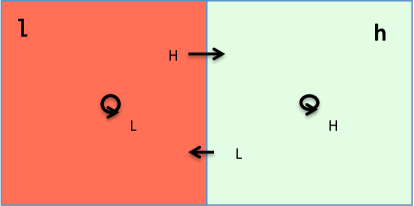
Figure 6: $SI$ in two quadrants

The application of the translation to the specification of Example 1 generates an agent model with 8 states, say ${\cal S}_{\Delta}=\{SA,SB,SC,SD,IA,IB,IC,ID\}$ with associated IDTMC probability transition matrix as shown in Figure 7 where $m_{\_}{xy}$ represents the fraction of objects currently in state $xy$ for $x\in\{S,I\}$ and $y\in\{A,B,C,D\}$—i.e. the components in state $x$ and with $\mathsf{loc}=y$ in the original specification of Fig 2—so that $\mathbf{m}=(m_{\_}{SA},m_{\_}{SB},m_{\_}{SC},m_{\_}{SD},m_{\_}{IA},m_{\_}{IB},m_{\_}{IC},m_{\_}{ID})$ is the occupancy measure vector. In Figure 7, functions $\phi_{\_}S$ and $\phi_{\_}I$ are used as abbreviations in the obvious way: $\phi_{\_}S(\mathbf{m})=m_{\_}{SA}+m_{\_}{SB}+m_{\_}{SC}+m_{\_}{SD}$ and $\phi_{\_}I(\mathbf{m})=m_{\_}{IA}+m_{\_}{IB}+m_{\_}{IC}+m_{\_}{ID}$. Let us assume now that we are interested in checking PCTL formulas on the model of Fig 2 which distinguish components located in $A$ or $C$ from those located in $B$ or $D$, and those in state $S$ from those in state $I$, that is we consider atomic propositions $Sh,Ih,Sl$ and $Il$ and a labelling ${\cal L}$ such that ${\cal L}(SA)={\cal L}(SC)=\{Sh\}$, ${\cal L}(IA)={\cal L}(IC)=\{Ih\}$, ${\cal L}(SB)={\cal L}(SD)=\{Sl\}$, and ${\cal L}(IB)={\cal L}(ID)=\{Il\}$.

$$\begin{array}[]{ c | c | c | c | c | c | c | c | c |}&SA&SB&SC&SD&IA&IB&IC&ID\\ \hline\cr SA&H\phi_{\_}S(\mathbf{m})&\frac{L}{2}\phi_{\_}S(\mathbf{m})&0&\frac{L}{2}\phi_{\_}S(\mathbf{m})&H\phi_{\_}I(\mathbf{m})&\frac{L}{2}\phi_{\_}I(\mathbf{m})&0&\frac{L}{2}\phi_{\_}I(\mathbf{m})\\ \hline\cr SB&\frac{H}{2}\phi_{\_}S(\mathbf{m})&L\phi_{\_}S(\mathbf{m})&\frac{H}{2}\phi_{\_}S(\mathbf{m})&0&\frac{H}{2}\phi_{\_}I(\mathbf{m})&L\phi_{\_}I(\mathbf{m})&\frac{H}{2}\phi_{\_}I(\mathbf{m})&0\\ \hline\cr SC&0&\frac{L}{2}\phi_{\_}S(\mathbf{m})&H\phi_{\_}S(\mathbf{m})&\frac{L}{2}\phi_{\_}S(\mathbf{m})&0&\frac{L}{2}\phi_{\_}I(\mathbf{m})&H\phi_{\_}I(\mathbf{m})&\frac{L}{2}\phi_{\_}I(\mathbf{m})\\ \hline\cr SD&\frac{H}{2}\phi_{\_}S(\mathbf{m})&0&\frac{H}{2}\phi_{\_}S(\mathbf{m})&L\phi_{\_}S(\mathbf{m})&\frac{H}{2}\phi_{\_}I(\mathbf{m})&0&\frac{H}{2}\phi_{\_}I(\mathbf{m})&L\phi_{\_}I(\mathbf{m})\\ \hline\cr IA&Hir&\frac{L}{2}ir&0&\frac{L}{2}ir&Hii&\frac{L}{2}ii&0&\frac{L}{2}ii\\ \hline\cr IB&\frac{H}{2}ir&Lir&\frac{H}{2}ir&0&\frac{H}{2}ii&Lii&\frac{H}{2}ii&0\\ \hline\cr IC&0&\frac{L}{2}ir&Hir&\frac{L}{2}ir&0&\frac{L}{2}ii&Hii&\frac{L}{2}ii\\ \hline\cr ID&\frac{H}{2}ir&0&\frac{H}{2}ir&Lir&\frac{H}{2}ii&0&\frac{H}{2}ii&Lii\\ \hline\cr\end{array}$$

Figure 7: IDTMC transition probability matrix $\mathbf{K}({\mathbf{m}})$, for ${\mathbf{m}}$ in ${\cal U}^{8}$.

Consider relation $R$ on ${\cal S}_{\Delta}$ defined as $R=I_{\_}{{{\cal S}_{\Delta}}}\cup\{(SA,SC),(SB,SD),(IA,IC),(IB,ID)\}\cup\{(SC,SA),\\ (SD,SB),(IC,IA),(ID,IB)\}$ where $I_{\_}{{{\cal S}_{\Delta}}}$ is the identity relation on ${\cal S}_{\Delta}$. It is very easy to show that $R$ is a bisimulation according to Definition 1. Clearly $R$ is an equivalence relation and its quotient ${\cal S}_{\Delta}/R$ is the set $\{Q_{\_}{Sh},Q_{\_}{Sl},Q_{\_}{Ih},Q_{\_}{Il}\}$ with $Q_{\_}{Sh}=\{SA,SC\},Q_{\_}{Sl}=\{SB,SD\},Q_{\_}{Ih}=\{IA,IC\},Q_{\_}{Il}=\{IB,ID\}$. In addition, for all $z_{\_}1,z_{\_}2\in{\cal S}_{\Delta}$, whenever $z_{\_}1\,R\,z_{\_}2$, we have ${\cal L}(z_{\_}1)={\cal L}(z_{\_}2)$ and $\mathbf{K}({\mathbf{m}})_{\_}{z_{\_}1,Q}=\mathbf{K}({\mathbf{m}})_{\_}{z_{\_}2,Q}$ for all $Q\in{\cal S}_{\Delta}/R$ and for all ${\mathbf{m}}$, as one can easily check; clearly, $R$ is also the largest bisimulation relation on ${\cal S}_{\Delta}$. The relationship between the two occupancy measure vectors is: $m_{\_}{{Q_{\_}{Sh}}}=m_{\_}{SA}+m_{\_}{SC}$, $m_{\_}{{Q_{\_}{Sl}}}=m_{\_}{SB}+m_{\_}{SD}$, $m_{\_}{{Q_{\_}{Ih}}}=m_{\_}{IA}+m_{\_}{IC}$, and $m_{\_}{{Q_{\_}{Il}}}=m_{\_}{IB}+m_{\_}{ID}$. We can thus use the reduced IDTMC defined by matrix $\widehat{\mathbf{K}}(m_{\_}{{Q_{\_}{Sh}}},m_{\_}{{Q_{\_}{Sl}}},m_{\_}{{Q_{\_}{Ih}}},m_{\_}{{Q_{\_}{Il}}})$ shown in Figure 9. It corresponds to the FlyFast agent specification $\widehat{\Delta}$ given in Figure 8. In a sense, the high probability locations $A$ and $C$, in the new model, have collapsed into a single one, namely $h$ and the low probability ones ($B$ and $D$) have collapsed into $l$, as shown in Figure 6. We point out again the correspondence between the symmetry in the space jump probability on one side and the definition of the state labelling function on the other side. Finally, note that a coarser labelling like, e.g. ${\cal L}^{\prime}(SA)={\cal L}^{\prime}(SC)={\cal L}^{\prime}(IA)={\cal L}^{\prime}(IC)=\{h\}$, ${\cal L}^{\prime}(SB)={\cal L}^{\prime}(SD)={\cal L}^{\prime}(IB)={\cal L}^{\prime}(ID)=\{l\}$ would make the model collapse into one with only two states, $Q_{\_}h$ and $Q_{\_}l$, with probabilities $H:Q_{\_}h\rightarrow Q_{\_}h,H:Q_{\_}l\rightarrow Q_{\_}h$, $L:Q_{\_}h\rightarrow Q_{\_}l$ and $L:Q_{\_}h\rightarrow Q_{\_}l$ where only the location would be modelled whereas information on the infection status would be lost.

action QSh_inf_QIh: H*(frc(QIh)+frc(QIl));ΨΨ        action QSh_nsc_QSh: H*(frc(QSh)+frc(QSl));
action QSh_inf_QIl: L*(frc(QIh)+frc(QIl));ΨΨ        action QSh_nsc_QSl: L*(frc(QSh)+frc(QSl));
action QSl_inf_QIh: H*(frc(QIh)+frc(QIl));ΨΨ        action QSl_nsc_QSh: H*(frc(QSh)+frc(QSl));
action QSl_inf_QIl: L*(frc(QIh)+frc(QIl));ΨΨ        action QSl_nsc_QSl: L*(frc(QSh)+frc(QSl));

action QIh_inf_QIh: H*ii;                          action QIh_rec_QSh: H*ir;
action QIh_inf_QIl: L*ii;                          action QIh_rec_QSl: L*ir;
action QIl_inf_QIh: H*ii;                          action QIl_rec_QSh: H*ir;
action QIl_inf_QIl: L*ii;                          action QIl_rec_QSl: L*ir;

state QSh{QSh_inf_QIh.QIh + QSh_inf_QIl.QIl + QSh_nsc_QSh.QSh + QSh_nsc_QSl.QSl}
state QSl{QSl_inf_QIh.QIh + QSl_inf_QIl.QIl + QSl_nsc_QSh.QSh + QSl_nsc_QSl.QSl}
state QIh{QIh_inf_QIh.QIh + QIh_inf_QIl.QIl + QIh_rec_QSh.QSh + QIh_rec_QSl.QSl}
state QIl{QIl_inf_QIh.QIh + QIl_inf_QIl.QIl + QIl_rec_QSh.QSh +QIl_rec_QSl.QSl}

Figure 8: Reduced agent specification $\widehat{\Delta{}}$

$$\begin{array}[]{ c | c | c | c | c |}&Q_{\_}{Sh}&Q_{\_}{Sl}&Q_{\_}{Ih}&Q_{\_}{Il}\\ \hline\cr Q_{\_}{Sh}&H\cdot(m_{\_}{{Q_{\_}{Sh}}}+m_{\_}{{Q_{\_}{Sl}}})&L\cdot(m_{\_}{{Q_{\_}{Sh}}}+m_{\_}{{Q_{\_}{Sl}}})&H\cdot(m_{\_}{{Q_{\_}{Ih}}}+m_{\_}{{Q_{\_}{Il}}})&L\cdot(m_{\_}{{Q_{\_}{Ih}}}+m_{\_}{{Q_{\_}{Il}}})\\ \hline\cr Q_{\_}{Sl}&H\cdot(m_{\_}{{Q_{\_}{Sh}}}+m_{\_}{{Q_{\_}{Sl}}})&L\cdot(m_{\_}{{Q_{\_}{Sh}}}+m_{\_}{{Q_{\_}{Sl}}})&H\cdot(m_{\_}{{Q_{\_}{Ih}}}+m_{\_}{{Q_{\_}{Il}}})&L\cdot(m_{\_}{{Q_{\_}{Ih}}}+m_{\_}{{Q_{\_}{Il}}})\\ \hline\cr Q_{\_}{Ih}&H\cdot ir&L\cdot ir&H\cdot ii&L\cdot ii\\ \hline\cr Q_{\_}{Il}&H\cdot ir&L\cdot ir&H\cdot ii&L\cdot ii\\ \hline\cr\end{array}$$

Figure 9: IDTMC transition probability matrix function $\widehat{\mathbf{K}}({\mathbf{m}})$, for ${\mathbf{m}}$ in ${\cal U}^{4}$.

7 Conclusions

PiFF [10] is a language for a predicate-based front-end of FlyFast, an on-the-fly mean-field model-checking tool. In this paper we presented a simplified version of the translation proposed in [10] together with an approach for model reduction that can be applied to the result of the translation. The approach is based on probabilistic bisimilarity for inhomogeneous DTMCs. An example of application of the procedure has been shown. The implementation of a compiler for PiFF mapping the language to FlyFast is under development as an add-on of FlyFast. We plan to apply the resulting extended tool to more as well as more complex models, in order to get concrete insights on the practical applicability of the framework and on the actual limitations imposed by the restrictions necessary for exploiting bisimilarity-based state-space reduction. Investigating possible ways of relaxing some of such restrictions will also be an interesting line of research.

Acknowledgments Research partially funded by EU Project n. 600708 A Quantitative Approach to Management and Design of Collective and Adaptive Behaviours (QUANTICOL).

Appendix A Appendix

Proof of Proposition 1
$\Leftarrow$: Trivial.
$\Rightarrow$:
We first prove that $a=b$:

$\noindent\hskip 14.45377pt\vspace{0.1in}\forall m_{\_}1,\ldots,m_{\_}S.A(m_{\_}1,\ldots,m_{\_}S)=B(m_{\_}1,\ldots,m_{\_}S)\newline \Rightarrow\hskip 18.06749pt\{$Logic$\}\vspace{0.1in}\newline \hskip 14.45377pt\vspace{0.1in}A(0,\ldots,0)=B(0,\ldots,0)\newline \Rightarrow\hskip 18.06749pt\{$Def. of $A(m_{\_}1,\ldots,m_{\_}S)$ and $B(m_{\_}1,\ldots,m_{\_}S)$$\}\vspace{0.1in}\newline \hskip 14.45377pt\vspace{0.1in}a=b$

Now we prove that $a_{\_}{ii}=b_{\_}{ii}$ for $i=1,\ldots,S$:

$\noindent\hskip 14.45377pt\vspace{0.1in}\forall m_{\_}1,\ldots,m_{\_}S.A(m_{\_}1,\ldots,m_{\_}S)=B(m_{\_}1,\ldots,m_{\_}S)\newline \Rightarrow\hskip 18.06749pt\{$Take the $S-tuple$ $(\bar{m}_{\_}1,\ldots,\bar{m}_{\_}S)$ where $\bar{m}_{\_}k=1$ if $k=i$ and $0$ otherwise$\}\vspace{0.1in}\newline \hskip 14.45377pt\vspace{0.1in}A(\bar{m}_{\_}1,\ldots,\bar{m}_{\_}S)=B(\bar{m}_{\_}1,\ldots,\bar{m}_{\_}S)\newline \Rightarrow\hskip 18.06749pt\{$Def. of $A(m_{\_}1,\ldots,m_{\_}S)$ and $B(m_{\_}1,\ldots,m_{\_}S)$$\}\vspace{0.1in}\newline \hskip 14.45377pt\vspace{0.1in}a_{\_}{ii}+a=b_{\_}{ii}+b\newline \Rightarrow\hskip 18.06749pt\{$$a=b$ (see above)$\}\vspace{0.1in}\newline \hskip 14.45377pt\vspace{0.1in}a_{\_}{ii}=b_{\_}{ii}$

Finally we prove that $a_{\_}{ij}=b_{\_}{ij}$, for $i,j=1,\ldots,S,j>i$:

$\noindent\hskip 14.45377pt\vspace{0.1in}\forall m_{\_}1,\ldots,m_{\_}S.A(m_{\_}1,\ldots,m_{\_}S)=B(m_{\_}1,\ldots,m_{\_}S)\newline \Rightarrow\hskip 18.06749pt\{$$(\tilde{m}_{\_}1,\ldots,\tilde{m}_{\_}S)$ where $\tilde{m}_{\_}k=0.5$ if $k\in\{i,j\}$ and $0$ otherwise$\}\vspace{0.1in}\newline \hskip 14.45377pt\vspace{0.1in}A(\tilde{m}_{\_}1,\ldots,\tilde{m}_{\_}S)=B(\tilde{m}_{\_}1,\ldots,\tilde{m}_{\_}S)\newline \Rightarrow\hskip 18.06749pt\{$Def. of $A(m_{\_}1,\ldots,m_{\_}S)$ and $B(m_{\_}1,\ldots,m_{\_}S)$$\}\vspace{0.1in}\newline \hskip 14.45377pt\vspace{0.1in}0.25a_{\_}{ii}+0.25a_{\_}{ij}+0.25a_{\_}{jj}+a=0.25b_{\_}{ii}+0.25b_{\_}{ij}+0.25b_{\_}{jj}+b\newline \Rightarrow\hskip 18.06749pt\{$$a=b$ (see above)$\}\vspace{0.1in}\newline \hskip 14.45377pt\vspace{0.1in}0.25a_{\_}{ii}+0.25a_{\_}{ij}+0.25a_{\_}{jj}=0.25b_{\_}{ii}+0.25b_{\_}{ij}+0.25b_{\_}{jj}\newline \Rightarrow\hskip 18.06749pt\{$Algebra$\}\vspace{0.1in}\newline \hskip 14.45377pt\vspace{0.1in}a_{\_}{ii}+a_{\_}{ij}+a_{\_}{jj}=b_{\_}{ii}+b_{\_}{ij}+b_{\_}{jj}\newline \Rightarrow\hskip 18.06749pt\{$$a_{\_}{ii}=b_{\_}{ii}$ and $a_{\_}{jj}=b_{\_}{jj}$ (see above)$\}\vspace{0.1in}\newline \hskip 14.45377pt\vspace{0.1in}a_{\_}{ij}=b_{\_}{ij}$ $\bullet$

References

- [1]
- [2] Adnan Aziz, Kumud Sanwal, Vigyan Singhal & Robert K. Brayton (2000): Model-checking continous-time Markov chains. ACM Trans. Comput. Log. 1(1), pp. 162–170, 10.1145/343369.343402.
- [3] Christel Baier, Boudewijn R. Haverkort, Holger Hermanns & Joost-Pieter Katoen (2003): Model-Checking Algorithms for Continuous-Time Markov Chains. IEEE Trans. Software Eng. 29(6), pp. 524–541, 10.1109/TSE.2003.1205180.
- [4] Christel Baier & Joost-Pieter Katoen (2008): Principles of model checking. MIT Press.
- [5] Girish Bhat, Rance Cleaveland & Orna Grumberg (1995): Efficient On-the-Fly Model Checking for CTL*. In: Proceedings, 10th Annual IEEE Symposium on Logic in Computer Science, San Diego, California, USA, June 26-29, 1995, IEEE Computer Society, pp. 388–397, 10.1109/LICS.1995.523273.
- [6] L. Bortolussi, G. Cabri, G. Di Marzo Serugendo, V. Galpin, J. Hillston, R. Lanciani, M. Massink & D. Tribastone, M. Weyns (2015): Verification of CAS. In J. Hillston, J. Pitt, M. Wirsing & F. Zambonelli, editors: Collective Adaptive Systems: Qualitative and Quantitative Modelling and Analysis, Schloss Dagstuhl - Leibniz-Zentrum für Informatik, Dagstuhl Publishing, Germany, pp. 91–102. Dagstuhl Reports. Vol. 4, Issue 12. Report from Dagstuhl Seminar 14512. ISSN 2192-5283.
- [7] Luca Bortolussi & Jane Hillston (2012): Fluid Model Checking. In Maciej Koutny & Irek Ulidowski, editors: CONCUR 2012 - Concurrency Theory - 23rd International Conference, CONCUR 2012, Newcastle upon Tyne, UK, September 4-7, 2012. Proceedings, Lecture Notes in Computer Science 7454, Springer, pp. 333–347, 10.1007/978-3-642-32940-124.
- [8] Luca Bortolussi & Jane Hillston (2015): Model checking single agent behaviours by fluid approximation. Inf. Comput. 242, pp. 183–226, 10.1016/j.ic.2015.03.002.
- [9] Jean-Yves Le Boudec, David D. McDonald & Jochen Mundinger (2007): A Generic Mean Field Convergence Result for Systems of Interacting Objects. In: Fourth International Conference on the Quantitative Evaluaiton of Systems (QEST 2007), 17-19 September 2007, Edinburgh, Scotland, UK, IEEE Computer Society, pp. 3–18, 10.1109/QEST.2007.8.
- [10] Vincenzo Ciancia, Diego Latella & Mieke Massink (2016): On-the-Fly Mean-Field Model-Checking for Attribute-Based Coordination. In Alberto Lluch-Lafuente & José Proença, editors: Coordination Models and Languages - 18th IFIP WG 6.1 International Conference, COORDINATION 2016, Held as Part of the 11th International Federated Conference on Distributed Computing Techniques, DisCoTec 2016, Heraklion, Crete, Greece, June 6-9, 2016, Proceedings, Lecture Notes in Computer Science 9686, Springer, pp. 67–83, 10.1007/978-3-319-39519-75.
- [11] Costas Courcoubetis, Moshe Y. Vardi, Pierre Wolper & Mihalis Yannakakis (1992): Memory-Efficient Algorithms for the Verification of Temporal Properties. Formal Methods in System Design 1(2/3), pp. 275–288, 10.1007/BF00121128.
- [12] R.W.R. Darling & J.R. Norris (2008): Differential equation approximations for Markov chains. Probability Surveys 5, pp. 37–79, 10.1214/07-PS121.
- [13] Rocco De Nicola, Diego Latella, Alberto Lluch-Lafuente, Michele Loreti, Andrea Margheri, Mieke Massink, Andrea Morichetta, Rosario Pugliese, Francesco Tiezzi & Andrea Vandin (2015): The SCEL Language: Design, Implementation, Verification. In Martin Wirsing, Matthias M. Hölzl, Nora Koch & Philip Mayer, editors: Software Engineering for Collective Autonomic Systems - The ASCENS Approach, Lecture Notes in Computer Science 8998, Springer, pp. 3–71, 10.1007/978-3-319-16310-91.
- [14] Giuseppe Della Penna, Benedetto Intrigila, Igor Melatti, Enrico Tronci & Marisa Venturini Zilli (2004): Bounded Probabilistic Model Checking with the Muralpha Verifier. In Alan J. Hu & Andrew K. Martin, editors: Formal Methods in Computer-Aided Design, 5th International Conference, FMCAD 2004, Austin, Texas, USA, November 15-17, 2004, Proceedings, Lecture Notes in Computer Science 3312, Springer, pp. 214–229, 10.1007/978-3-540-30494-416.
- [15] Cheng Feng & Jane Hillston (2014): PALOMA: A Process Algebra for Located Markovian Agents. In Gethin Norman & William H. Sanders, editors: Quantitative Evaluation of Systems - 11th International Conference, QEST 2014, Florence, Italy, September 8-10, 2014. Proceedings, Lecture Notes in Computer Science 8657, Springer, pp. 265–280, 10.1007/978-3-319-10696-022.
- [16] Nicolas Gast & Bruno Gaujal (2010): A mean field model of work stealing in large-scale systems. In Vishal Misra, Paul Barford & Mark S. Squillante, editors: SIGMETRICS 2010, Proceedings of the 2010 ACM SIGMETRICS International Conference on Measurement and Modeling of Computer Systems, New York, New York, USA, 14-18 June 2010, ACM, pp. 13–24, 10.1145/1811039.1811042.
- [17] Stefania Gnesi & Franco Mazzanti (2011): An Abstract, on the Fly Framework for the Verification of Service-Oriented Systems. In Martin Wirsing & Matthias M. Hölzl, editors: Rigorous Software Engineering for Service-Oriented Systems - Results of the SENSORIA Project on Software Engineering for Service-Oriented Computing, Lecture Notes in Computer Science 6582, Springer, pp. 390–407, 10.1007/978-3-642-20401-218.
- [18] Guillaume Guirado, Thomas Hérault, Richard Lassaigne & Sylvain Peyronnet (2006): Distribution, Approximation and Probabilistic Model Checking. Electr. Notes Theor. Comput. Sci. 135(2), pp. 19–30, 10.1016/j.entcs.2005.10.016.
- [19] Ernst Moritz Hahn, Holger Hermanns, Björn Wachter & Lijun Zhang (2009): INFAMY: An Infinite-State Markov Model Checker. In Ahmed Bouajjani & Oded Maler, editors: Computer Aided Verification, 21st International Conference, CAV 2009, Grenoble, France, June 26 - July 2, 2009. Proceedings, Lecture Notes in Computer Science 5643, Springer, pp. 641–647, 10.1007/978-3-642-02658-449.
- [20] Hans Hansson & Bengt Jonsson (1994): A Logic for Reasoning about Time and Reliability. Formal Asp. Comput. 6(5), pp. 512–535, 10.1007/BF01211866.
- [21] Thomas Hérault, Richard Lassaigne, Frédéric Magniette & Sylvain Peyronnet (2004): Approximate Probabilistic Model Checking. In Bernhard Steffen & Giorgio Levi, editors: Verification, Model Checking, and Abstract Interpretation, 5th International Conference, VMCAI 2004, Venice, January 11-13, 2004, Proceedings, Lecture Notes in Computer Science 2937, Springer, pp. 73–84, 10.1007/978-3-540-24622-08.
- [22] Gerard J. Holzmann (2004): The SPIN Model Checker - primer and reference manual. Addison-Wesley.
- [23] D. Huynh & L. Tian (1992): On some equivalence relations for probabilistic processes. Fundamenta Informaticae 17, pp. 211–234.
- [24] A. Kolesnichenko, A. Remke & P.-T. de Boer (2012): A logic for model-checking of mean-field models. Technical Report TR-CTIT-12-11, http://doc.utwente.nl/80267/.
- [25] Anna Kolesnichenko, Pieter-Tjerk de Boer, Anne Remke & Boudewijn R. Haverkort (2013): A logic for model-checking mean-field models. In: 2013 43rd Annual IEEE/IFIP International Conference on Dependable Systems and Networks (DSN), Budapest, Hungary, June 24-27, 2013, IEEE Computer Society, pp. 1–12, 10.1109/DSN.2013.6575345.
- [26] Kim G. Larsen & Axel Legay (2016): Statistical Model Checking: Past, Present, and Future. In Tiziana Margaria & Bernhard Steffen, editors: Leveraging Applications of Formal Methods, Verification and Validation: Foundational Techniques - 7th International Symposium, ISoLA 2016, Imperial, Corfu, Greece, October 10-14, 2016, Proceedings, Part I, Lecture Notes in Computer Science 9952, pp. 3–15, 10.1007/978-3-319-47166-21.
- [27] D. Latella (1983): Comunicazione basata su proprietà nei sistemi decentralizzati. [Property-based inter-process communication in decentralized systems] Graduation Thesis. Istituto di Scienze dell’Informazione. Univ. of Pisa, Italy (in italian).
- [28] Diego Latella, Michele Loreti & Mieke Massink (2013): On-the-fly Fast Mean-Field Model-Checking. In Martín Abadi & Alberto Lluch-Lafuente, editors: Trustworthy Global Computing - 8th International Symposium, TGC 2013, Buenos Aires, Argentina, August 30-31, 2013, Revised Selected Papers, Lecture Notes in Computer Science 8358, Springer, pp. 297–314, 10.1007/978-3-319-05119-217.
- [29] Diego Latella, Michele Loreti & Mieke Massink (2014): On-the-fly Probabilistic Model Checking. In Ivan Lanese, Alberto Lluch-Lafuente, Ana Sokolova & Hugo Torres Vieira, editors: Proceedings 7th Interaction and Concurrency Experience, ICE 2014, Berlin, Germany, 6th June 2014., EPTCS 166, pp. 45–59, 10.4204/EPTCS.166.6.
- [30] Diego Latella, Michele Loreti & Mieke Massink (2015): On-the-fly PCTL fast mean-field approximated model-checking for self-organising coordination. Sci. Comput. Program. 110, pp. 23–50, 10.1016/j.scico.2015.06.009.
- [31] Michele Loreti & Jane Hillston (2016): Modelling and Analysis of Collective Adaptive Systems with CARMA and its Tools. In Marco Bernardo, Rocco De Nicola & Jane Hillston, editors: Formal Methods for the Quantitative Evaluation of Collective Adaptive Systems - 16th International School on Formal Methods for the Design of Computer, Communication, and Software Systems, SFM 2016, Bertinoro, Italy, June 20-24, 2016, Advanced Lectures, Lecture Notes in Computer Science 9700, Springer, pp. 83–119, 10.1007/978-3-319-34096-84.