KiDS-i-800: Comparing weak gravitational lensing measurements from same-sky surveys

Abstract

We present a weak gravitational lensing analysis of 815 square degree of $i$-band imaging from the Kilo-Degree Survey (KiDS-$i$-800). In contrast to the deep $r$-band observations, which take priority during excellent seeing conditions and form the primary KiDS dataset (KiDS-$r$-450), the complementary yet shallower KiDS-$i$-800 spans a wide range of observing conditions. The overlapping KiDS-$i$-800 and KiDS-$r$-450 imaging therefore provides a unique opportunity to assess the robustness of weak lensing measurements. In our analysis we introduce two new ‘null’ tests. The ‘nulled’ two-point shear correlation function uses a matched catalogue to show that the calibrated KiDS-$i$-800 and KiDS-$r$-450 shear measurements agree at the level of $1\pm 4$%. We use five galaxy lens samples to determine a ‘nulled’ galaxy-galaxy lensing signal from the full KiDS-$i$-800 and KiDS-$r$-450 surveys and find that the measurements agree to $7\pm 5$% when the KiDS-$i$-800 source redshift distribution is calibrated using either spectroscopic redshifts, or the 30-band photometric redshifts from the COSMOS survey.

1 Introduction

Weak gravitational lensing provides a powerful way to measure the total matter distribution. Light rays from background ‘source’ galaxies are deflected by massive foreground structures and the statistical measurement of these distortions allows for the detection of the gravitational potential of the foreground ‘lenses’. This gives information about cosmic geometry and the growth of large-scale structures in the Universe, without any prior assumptions about dark matter or galaxy bias (Hoekstra & Jain, 2008; Kilbinger, 2015).

As the lensing distortion of a single galaxy is typically much smaller than the intrinsic ellipticity, measurements require wide-area, deep, high-quality optical images. Some large optical surveys that have been exploited for weak lensing studies in the last decade are the Sloan Digital Sky Survey (SDSS; Mandelbaum et al., 2005), the Canada-France-Hawaii Telescope Legacy Survey (CFHTLenS; Heymans et al., 2012b), the Deep Lens Survey (DLS; Wittman et al., 2002) and the Red Sequence Cluster Survey (RCS and RCSLenS; van Uitert et al., 2011; Hildebrandt et al., 2016), as well as the on-going Dark Energy Survey (DES; Jarvis et al., 2016), the Hyper Supreme-Cam Survey (HSC; Aihara et al., 2017) and the Kilo-Degree Survey (KiDS; Kuijken et al., 2015). The non-trivial nature of weak lensing measurements, owing to their susceptibility to various systematics, stimulates a need for consistency checks between the lensing signals derived from unique datasets.

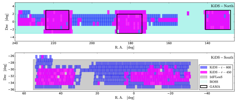
Figure 1: KiDS-$i$-800 survey footprint. Each purple box corresponds to a single KiDS $i$-band pointing of $1\text{\,}{\mathrm{deg}}^{2}$ and for comparison, each overplotted pink box corresponds to a KiDS-$r$-450 pointing. The cyan region indicates the BOSS spectroscopic coverage and the grey region in the South indicates the 2dFLenS spectroscopic coverage. The black outlined rectangles are the GAMA spectroscopic fields that overlap with the KiDS North field.

This paper presents the first lensing results using $815\text{\,}{\mathrm{deg}}^{2}$ of KiDS $i$-band imaging (hereafter referred to as KiDS-$i$-800), along with the first large-scale lensing analysis of two overlapping imaging surveys, where we make a detailed comparison to lensing measurements from $450\text{\,}{\mathrm{deg}}^{2}$ of $r$-band imaging (hereafter referred to as KiDS-$r$-450). KiDS is a multi-band, large-scale, imaging survey that seeks to unveil the properties of the evolving dark universe by tracing the density of clustered matter using weak lensing tomography. Its observations are taken in four broad-band filters (ugri) using the OmegaCAM at the VLT Survey Telescope (VST) at the European Southern Observatory’s Paranal Observatory (de Jong et al., 2013; Kuijken et al., 2015). Details of the KiDS-$r$-450 data reduction and subsequent cosmic shear analysis are presented in Hildebrandt et al. (2017).

The KiDS observing strategy is fashioned to provide optimal imaging for shape measurements in the $r$-band where the data are homogeneous in terms of limiting depth and low atmospheric seeing. In contrast, the $i$-band imaging encompasses a wide range of depth owing to its varied seeing conditions and sky brightness. Though these $i$-band images are highly variable in quality, if the redshift distribution can be sufficiently calibrated, the cosmological range in scale probed by the data available could be useful for cross-correlation studies such as galaxy-shear cross correlation, or galaxy-galaxy lensing (Hoekstra et al., 2004; Mandelbaum et al., 2005) and galaxy-CMB lensing (for an application of this technique see Hand et al., 2015). In addition, galaxy-galaxy lensing can be combined with galaxy clustering to shed light on the growth of structure (Leauthaud et al., 2017; Kwan et al., 2017), as well as with redshift-space distortions to test gravity (Blake et al., 2016a; Alam et al., 2017).

Furthermore, the areal overlap between these two shape catalogues allows for a unique consistency test of our shear and redshift estimates across different observing conditions and depths. The galaxy-galaxy lensing measurement of the excess surface mass density is invariant to the redshift of the source samples. As this measurement is also essentially insensitive to the assumed cosmology, this allows for a powerful systematic test (Mandelbaum et al., 2005; Heymans et al., 2012b). The excess surface mass density statistic is, however, sensitive to both errors in the shear calibration and redshift distributions and therefore cannot distinguish between these two sources of systematic error, providing only a joint calibration of the two effects. As such we employ a complementary ‘nulled’ two-point shear correlation test using a matched galaxy sample to independently identify calibration errors in the shear measurement.

The paper is organised as follows. Section 2 presents the survey outline, details the shape measurement pipeline and reviews the $i$-band data quality. An outline of the various methods for estimating the redshift distribution is given in Section 3. Section 4 compares the KiDS-$i$-800 dataset to the KiDS-$r$-450 dataset in terms of the nulled two-point shear correlation function and the the nulled galaxy-galaxy lensing signal of the datasets. That is, we explore the difference in shear only for galaxies measured in both bands, as well as the shape and photometry of all galaxies in each band. Finally, we summarise the outcomes of this study and the outlook in Section 5. In the Appendices we detail the differences in the data reduction process between KiDS-$r$-450 and KiDS-$i$-800 (Appendix A), the selection criteria we apply for galaxy-galaxy lensing (Appendix B), a comparison of our star selection with the Gaia survey (Appendix C), the corrections applied to the galaxy-galaxy lensing signal (Appendix D) and the computation of the analytical covariance for the nulled two-point shear correlation function (Appendix E).

2 Shear data

Both the OmegaCAM and the VST are specifically designed to be optimally suited for uniform and high-quality images over the one-square degree field of view. For a particular field in any of the $(u)gri$ filters, observations comprise (four) five dithered exposures in immediate succession.

The KiDS deep $r$-band images are observed in dark time with a total exposure time of 1800 seconds during the best-seeing conditions with FWHM$<$0.9 arcsec and a median FWHM of 0.66 arcsec (for the public data release, see de Jong et al., 2017). The $r$-band observations thus provide the primary images for weak lensing analyses (Kuijken et al., 2015; Hildebrandt et al., 2017). The $u$-band and $g$-band also use dark time with weaker seeing constraints. In contrast the $i$-band data is observed in bright time, with a shorter total exposure time of 1200 seconds, over a range of seeing conditions satisfying FWHM$<$ 1.2 arcsec, in this case with a median FWHM of 0.79 arcsec. The data collection rate for this variable seeing bright time data therefore surpasses that of the $ugr$ data. At present, the full 1500 square degree KiDS footprint is essentially complete in $i$-band, in contrast to the completed $ugr$ imaging which, as of January 2018, spans seventy percent of the final survey area. This enhanced areal $i$-band coverage, in comparison to the multi-band imaging, thus motivated our investigation into its use for weak lensing analyses.

The KiDS-$i$-800 dataset consists of all fields observed in the i-band filter before December 14th, 2014. These fields were analysed and subjected to a series of strict quality-control tests during the data reduction, as presented in Appendix A. This selection resulted in a dataset of 815 fields, hence the name ‘KiDS-$i$-800’. Out of these 815 fields, 381 have also undergone a weak lensing analysis in the $r$-band as part of the KiDS-$r$-450 data release.

Figure 1 shows the KiDS-$i$-800 coverage and the overlapping spectroscopic area with the Baryon Oscillation Spectroscopic Survey (Dawson et al., 2013, BOSS) and the Galaxy and Mass Assembly survey (Driver et al., 2011, GAMA) in the North. In the South, the 2-degree Field Lensing Survey (Blake et al., 2016b, 2dFLenS) is specifically designed as the spectroscopic follow-up of KiDS. The complete spectroscopic overlap between these datasets renders KiDS-$i$-800 an optimal survey for cross-correlation studies, such as galaxy-galaxy lensing.

2.1 Data reduction and Object Detection

The theli pipeline (Erben et al., 2005; Schirmer, 2013), developed from CARS (Erben et al., 2009) and CFHTLenS (Erben et al., 2013) and fully described in Kuijken et al. (2015), was used for a lensing-quality reduction of the KiDS-$i$-800 dataset. The basis of our theli processing starts with the removal of the instrumental signatures of OmegaCAM data provided by the ESO archive. Next, photometric zero-points, atmospheric extinction coefficients and colour terms are estimated per complete processing run and where necessary, we correct the OmegaCAM data for any evidence of electronic cross-talk between detectors on the images and fringing. Finally the sky is subtracted from each CCD in every exposure. Individual sky background models are created by SExtractor, adopting a filtering scale (BACKSIZE) of 512 pixels. All images from each KiDS pointing are astrometrically calibrated against the SDSS Data Release 12 (Alam et al., 2015) where available and the 2MASS catalogue (Skrutskie et al., 2006) otherwise. These calibrated images are co-added with a weighted mean algorithm. SExtractor (Bertin & Arnouts, 1996) is run on the co-added images to generate the source catalogue for the lensing measurements. Masks that cover image defects, reflections and ghosts, are also created (see Section 3.4 of Kuijken et al., 2015, for more details). An account of the differences between the data reduction for KiDS-$i$-800 and KiDS-$r$-450 is given in Appendix A. After masking and accounting for overlap between the tiles, the KiDS i-800 dataset spans an effective area of 733 square degree.

2.2 Modelling the Point Spread Function

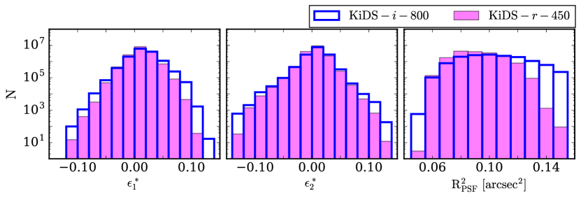
Figure 2: Comparison of the properties of the PSF model reconstructed at the position of each resolved galaxy in KiDS-$i$-800 (blue) and KiDS-$r$-450 (pink): The left-hand and middle panels show the distribution of each component of PSF ellipticity. The width of the KiDS-$i$-800 PSF ellipticity distribution is comparable to that of KiDS-$r$-450. The right-hand panel shows the distribution of the local PSF size illustrating the wider range of seeing conditions with KiDS-$i$-800 observations. Note that all panels have a log scaling to highlight the differences in the distribution of the KiDS $i$ and $r$-band data in the extremes.

Galaxy images are smeared as photons travel through the Earth’s atmosphere and further distorted due to telescope optics and detector imperfections. This gives rise to a spatially and temporally variable point spread function (PSF) that can be characterised and corrected for using star catalogues.

With high-resolution KiDS $r$-band imaging, star-galaxy separation can be reliably determined by inspecting the size and ‘peakiness’ of each object in each exposure. A star catalogue is then assembled by selecting the objects that group together in a distinct stellar peak and appear in three or more of the five exposures (see Section 3.2 of Kuijken et al., 2015, for details). For the variable seeing $i$-band imaging, however, we found this method to be unreliable, as in very poor seeing the stellar peak is no longer as distinct from the galaxy sample.

For KiDS-$i$-800 we first select stellar candidates automatically in the size-magnitude plane (see Section 4 of Erben et al., 2013, for details). We estimate the complex ellipticity of each stellar candidate, from each exposure, in terms of its weighted second order quadrupole moments $Q_{ij}$,

$$Q_{ij}=\frac{\int\mathrm{d}^{2}{\bf x}\,W({\bf|x|})\,I({\bf x})\,x_{i}\,x_{j}}{\int\mathrm{d}^{2}{\bf x}\,W({\bf|x|})\,I({\bf x})}\,,$$ (1)

where $I({\bf x})$ is the surface brightness of the object at position ${\bf x}$, measured from the SExtractor position and $W({\bf|x|})$ is a Gaussian weighting function with dispersion of three pixels, (following Kuijken et al., 2015), which we employ to suppress noise at large scales. The complex stellar ellipticity is then calculated from,

$$\epsilon^{\mathrm{*}}=\epsilon_{1}^{\mathrm{*}}+\mathrm{i}\epsilon_{2}^{\mathrm{*}}=\frac{Q_{11}-Q_{22}+2\mathrm{i}Q_{12}}{Q_{11}+Q_{22}+2\sqrt{Q_{11}Q_{22}-Q_{12}^{2}}}\,.$$ (2)

In the case of a perfect ellipse, the unweighted complex ellipticity $\epsilon$ (where $W({\bf|x|})=1$ for all ${\bf|x|}$), is related to the axial ratio $q$ and orientation of the ellipse $\phi$ as,

$$\epsilon=\epsilon_{1}+\mathrm{i}\epsilon_{2}=\left(\frac{1-q}{1+q}\right)\mathrm{e}^{2\mathrm{i}\phi}\,.$$ (3)

Using a second-order polynomial model, the spatially varying stellar ellipticity, or PSF, is modelled across each exposure. Outliers are rejected from the candidate sample if their measured ellipticities differ by more than $3\sigma$ from the local PSF model, where $\sigma^{2}$ is the variance of the PSF model ellipticity across the field of view. A final $i$-band star catalogue is then assembled from the cleaned stellar candidate lists by again requiring that the stellar object has been selected in three or more exposures.

In Appendix C we investigate the robustness of our two different star-galaxy selection methods in both the $i$ and $r$-bands by comparing our star catalogues to the stellar catalogues published by the Gaia mission in their first data release (Gaia Collaboration et al., 2016). We find that, considering objects brighter than $i<20$, our $i$-band stellar selection rejects 14 percent of unsaturated Gaia sources compared to our $r$-band stellar selection which rejects 10 percent.

In principle, our star selection could yield an unrepresentative sample of stars, leading to an error in the PSF model. In order to inspect the quality of the PSF modelling for the exposures of each field, we therefore compute the residual PSF ellipticty, $\delta\epsilon^{*}=\epsilon^{*}(\rm{model})-\epsilon^{*}(\rm{data})$. For an accurate PSF model, this should be dominated by photon noise and therefore be uncorrelated between neighbouring stars. An investigation into the two-point $i$-band PSF residual ellipticity correlation function, $\langle\delta\epsilon^{*}\overline{\delta\epsilon}^{*}\rangle$, where the bar denotes the complex conjugate, revealed that this statistic was consistent with zero between the angular scales of 0.8 arcmin to 60 arcmin. From this we can conclude that the PSF model accurately predicts the amplitude and angular dependence of the two-point PSF ellipticity correlation function. The same conclusion was drawn in the assessment of the $r$-band imaging in Kuijken et al. (2015).

Figure 2 compares the PSF model properties of the KiDS-$i$-800 and KiDS-$r$-450 data. The left and middle panels show the number of resolved galaxies, in each dataset, as a function of the model PSF ellipticity $\epsilon^{*}$ at the location of the galaxy. We find that the spread of PSF ellipticities in the $i$-band is comparable to that of KiDS-$r$-450, with slightly more instances of higher-ellipticity PSFs in the tails of the distribution.

The right panel of Figure 2 shows the distribution of the local PSF size at the positions of resolved galaxies, where the PSF size is determined in terms of the quadrupole moments, $Q_{ij}$, as

$${R_{\rm{PSF}}^{2}}=\sqrt{Q_{11}Q_{22}-Q_{12}^{2}}\,.$$ (4)

This panel illustrates the wider range of seeing conditions within the $i$-band dataset, in comparison to the more homogeneous KiDS-$r$-450 data. Note that we examined how the ellipticity of the $i$-band PSF varied with worsening seeing conditions but found that these two quantities were largely uncorrelated.

2.3 Galaxy shape measurement and selection

Galaxy shapes were measured using lensfit, a likelihood based model-fitting method that fits PSF-convolved bulge-plus-disk galaxy models to each exposure simultaneously in order to estimate the shear (Miller et al., 2013). In this analysis, we adopt the latest ‘self-calibrating’ version of lensfit (Fenech Conti et al., 2017). As any single point measurement of galaxy ellipticity is biased by pixel noise in the image, this upgraded version is designed to mitigate these effects based on the actual measurements and an extensive suite of image simulations . In addition, weights are recalibrated in order to correct for biases that arise due to the relative orientation of the PSF and the galaxy, as highlighted by Miller et al. (2013), and a revised de-blending algorithm is adopted in order to reject fewer galaxies that are too close to their nearest neighbour. We refer the reader to Section 2.5 of Hildebrandt et al. (2017) for a comprehensive list of the advances on the version of the algorithm used in previous analyses, such as Kuijken et al. (2015). This version of lensfit leaves a percent-level residual multiplicative noise bias, which we parametrise using image simulations. It was demonstrated in Fenech Conti et al. (2017) that model bias contributes at the per mille level for a KiDS-like survey when tested with simulations of COSMOS galaxies (Voigt & Bridle, 2010).

We account for the intrinsic differences between the $i$ and $r$-band galaxy populations by adopting different priors on galaxy size for the $i$ and $r$-band lensfit analyses (Kuijken et al., 2015). We do, however, assume the distribution of galaxy ellipticities and the bulge-to-disk ratio are the same for both bands. Hildebrandt et al. (2016) found that using an $i$-band size prior to analyse $r$-band data using lensfit resulted in an average change in the observed galaxy ellipticity of less than 1 percent. This demonstrates that we do not require high levels of accuracy in the determination of the galaxy size prior in each band.

Using an extensive suite of $r$-band image simulations, Fenech Conti et al. (2017) show that lensfit provides shear estimates that are accurate at the percent level. We use these results to calibrate a possible residual multiplicative shear measurement bias, $m$, in the $i$-band observations. We note two important caveats, however, that the Fenech Conti et al. (2017) image simulations did not explore: the extreme PSF sizes found in KiDS-$i$-800 and an $i$-band galaxy population. As the calibration corrections are determined as a function of galaxy resolution, that is, the ratio of the galaxy size and the PSF size, and because the $r$-band galaxy population is similar to the $i$-band population, we expect the conclusions from Fenech Conti et al. (2017) to apply to $i$-band observations. We note that any high- accuracy science, for example cosmic shear, using KiDS-$i$-800 would, however, require independent verification of the $i$-band calibration corrections adopted in this analysis.

The Fenech Conti et al. (2017) image simulation analysis was limited to galaxies fainter than $r>20$. Providing a calibration correction below this magnitude would require an extension to the image simulation pipeline, as these bright galaxies typically extend beyond the standard simulated postage stamp size. By comparing galaxies in $r-i$ colour space we determined an equivalent $i$-band limit to be $i>19.4$, limiting our $i$-band analysis to galaxies fainter than this threshold.

Each lensfit ellipticity measurement is accompanied by an inverse variance weight that is set to zero when the object is unresolved or point-like, for example. Requiring that shapes have a non-zero lensfit weight therefore effectively removes stars and faint unresolved galaxies. The 0.01$\%$ of objects that were deemed by their ‘fitclass’ value to be poorly fit by a bulge-plus-disk galaxy model were also removed, effectively removing any image defects that entered the object detection catalogue (see Section D1 of Hildebrandt et al., 2017, for details). We note that without multi-colour information we were unable to detect and remove faint satellite or asteroid trails in the $i$-band, or identify any moving sources from the individual exposures, which were shown in Hildebrandt et al. (2017) to be a significant contaminating source for some fields of the $r$-band data analysis. While this would be important for the case of cosmic shear, these artefacts have a negligible effect for cross-correlation studies.

We investigated how the average ellipticity of the galaxy sample varied when applying progressively more conservative cuts on our de-blending parameter, the contamination radius. This is a measure of the distance to neighbouring galaxies and therefore the contaminating light in the image of the main galaxy. We found that the average ellipticity of the full sample converged when galaxies with a contamination radius greater than 4.25 pixels were selected. Hildebrandt et al. (2017) also concluded that a de-blending selection criterion of 4.25 pixels was optimal for the $r$-band imaging.

2.4 Calibrating KiDS galaxy shapes

Observed galaxy images are convolved with the PSF and pixellated. They are also inherently noisy and in order to deal with the residual noise bias, shear measurements typically require calibration corrections with a suite of image simulations. Corrections to the observed shear estimator, $\epsilon^{\mathrm{obs}}$ can be modelled in terms of a multiplicative shear term $m$, a multiplicative PSF model term $\alpha\epsilon^{*}=\alpha_{1}\epsilon_{1}^{*}+\mathrm{i}\alpha_{2}\epsilon_{2}^{*}$, a PSF modelling error term $\beta\delta\epsilon^{\mathrm{*}}$, and an additive term, $c=c_{1}+\mathrm{i}c_{2}$, that is uncorrelated with the PSF, such that

$$\epsilon^{\mathrm{obs}}=\left(\frac{\epsilon^{\mathrm{int}}+\gamma}{1+\bar{\gamma}\epsilon^{\mathrm{int}}}\right)(1+m)+\epsilon^{\mathrm{n}}+\alpha\epsilon^{\mathrm{*}}+\beta\,\delta\epsilon^{\mathrm{*}}+c\,.$$ (5)

Here all quantities are complex (see equation 3), with the exception of the multiplicative calibration scalars $m$ and $\beta$. The first bracketed term transforms the galaxy’s intrinsic ellipticity $\epsilon^{\mathrm{int}}$ by $\gamma$, the reduced lensing-induced shear that we wish to detect (Seitz & Schneider, 1997). In this analysis we take the weak lensing approximation that the reduced shear and the shear are equal and use the notation $\bar{\gamma}$, to indicate a complex conjugate. $\epsilon^{\mathrm{n}}$ is the random noise on the measured galaxy ellipticity which will increase as the signal-to-noise of the galaxy decreases (Viola et al., 2014), and $\epsilon^{\mathrm{*}}$ is the ellipticity of the true PSF. For a perfect shape measurement method, $m,c$ and $\alpha\epsilon^{\mathrm{*}}$ would all be zero and for a perfect PSF model $\beta\,\delta\epsilon^{\mathrm{*}}$ would also be zero (Hoekstra, 2004; Heymans et al., 2006).

In this analysis we use the PSF model as a proxy for the true PSF, in which case the $\beta$ becomes subsumed into $\alpha$, the PSF contamination. This is appropriate given that the measured PSF ellipticity residual correlation function $\langle\delta\epsilon^{*}\overline{\delta\epsilon}^{*}\rangle$, was found to be consistent with zero (see Section 2.2). The additive calibration correction $c$ and PSF term $\alpha$ can then be estimated empirically by fitting the model in equation 5 directly to the data assuming that the data volume is sufficiently large such that the average $\langle\gamma+\epsilon^{\mathrm{int}}\rangle=0$. For KiDS-$i$-800 we find that $c_{1}=-0.0011\pm 0.0001$, $c_{2}=0.0018\pm 0.0001$, $\alpha_{1}=0.067\pm 0.006$ and $\alpha_{2}=0.074\pm 0.006$. As with a similar analysis for KiDS-$r$-450, we find measurements of $\alpha$ to be uncorrelated with $c$.

In Figure 3 we show the measured additive calibration correction $c$ and PSF term $\alpha$ for the Northern and Southern KiDS-$i$-800 patches as a function of the observed PSF size, $R_{\rm{PSF}}^{2}$ (equation 4). We find that the $i$-band PSF contamination is significant (even when the $i$-band data are restricted to the same seeing range as the $r$-band), in comparison to the case of KiDS-r-450, where the PSF contamination in each tomographic bin and survey patch ranged between $-0.03<\alpha<0.02$ with an error $\sim 0.01$ (for further details see Section D4 of Hildebrandt et al. 2017). As the PSF ellipticity distributions between the two bands are comparable (see Figure 2), the fact that we find different levels of PSF contamination between the $i$ and $r$-band images could lead to a better understanding of how differences in the data reduction and analysis lead to a PSF error. The primary difference between the KiDS-$i$-800 and KiDS-$r$-450 data reduction in the Southern field is the method used to determine the astrometric solution. In KiDS-$i$-800, this was determined for each pointing individually, whereas an improved full global solution was derived for the $r$-band. In the Northern patch, however, astrometry for both KiDS-$i$-800 and KiDS-$r$-450 was tied to SDSS (Alam et al., 2015). With similar levels of PSF contamination in the Northern and Southern KiDS-$i$-800 patches as demonstrated in Figure 3, we can conclude that astrometry is likely not to be at the root of this issue. The method to determine a stellar catalogue also differed (see Section 2.2). Our comparison to stellar catalogues from Gaia in Appendix C suggests that a selection bias could have been introduced during star selection. With PSF residuals shown to be consistent with zero in Section 2.2, however, we can also conclude that PSF modelling is likely not to be at the root of this issue. The third main difference between the data sets is a non-negligible level of residual fringing in the KiDS-i-800 images (see the discussion in Appendix A). Residual fringe removal was not prioritised in the early stages of the KiDS-i-800 data reduction as the plan for this dataset did not include cosmic shear studies. As the fringe patterns are uncorrelated with the PSF, it is thought that fringing is unlikely to be the root cause of the PSF contamination, but this will be explored further in future analyses.

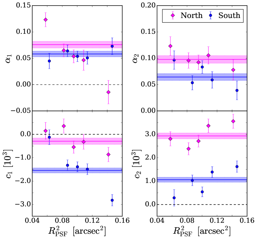
Figure 3: The variation of the additive bias term, $c$ (lower panel) and the multiplicative PSF model term, $\alpha$ (upper panel) with the size of the PSF. The analysis of the Northern fields are shown in pink and the Southern fields in blue. The solid line represents the mean of the data points and the coloured bands indicate a 1$\sigma$ deviation.

As the primary science goals for KiDS-$i$-800 is this demonstrative comparison, we decided to defer further studies of the origin of the $i$-band PSF contamination. For the galaxy-galaxy lensing comparison, any PSF contamination is effectively removed when azimuthal averages are taken around foreground lens structures. Additive biases are also accounted for by correcting the signal using the measured signal around random points (see Section 4.2). This level of PSF contamination renders KiDS-$i$-800 unsuitable for cosmic shear studies.

2.5 Matched $ri$ catalogue

We create a matched $r$ and $i$-band catalogue, limited to galaxies that have a shape measurement in both KiDS-$i$-800 and KiDS-$r$-450, using a $1\text{\,}\mathrm{arcsec}$ matching window. The overlapping $ri$ survey footprint has an effective area of $302\text{\,}{\mathrm{deg}}^{2}$, taking into account the area lost to masks. Only 39% of the $r$-band shape catalogue in this area is matched, which is expected as the effective number density of the $r$-band shear catalogues is more than double the effective number density of the $i$-band shear catalogues (see Section 4). 78% of the $i$-band shape catalogue is matched, however, and this number increases to 89% when an accurate $r$-band shape measurement is not required. We made a visual inspection of a sample of the remaining unmatched $i$-band objects revealing different de-blending choices between the $r$-band and $i$-band images, where the SExtractor object detection algorithm has chosen different centroids owing to the differing data quality between the two images. We also found differences in low signal-to-noise peaks, and a small fraction of objects with significant flux in the $i$-band but no significant $r$-band flux counterpart. We define a new weight for each member of this matched sample as a combination of the lensfit weights of the galaxy, assigned in the KiDS-$i$-800 sample, $w_{i}$ and in KiDS-$r$-450, $w_{r}$, with, $w^{ir}=\sqrt{w_{i}w_{r}}$. By combining the weights in this way we ensure that the effective weighted redshift distribution of the two matched samples is the same.

3 Redshift data

3.1 The spectroscopic lens samples

In our comparison study we present a galaxy-galaxy lensing analysis, where we select samples of lens galaxies from spectroscopic redshift surveys. As KiDS overlaps with a number of wide-field spectroscopic surveys, this choice reduces the error associated with the alternative approach of defining a photometric redshift selected lens sample (see for example Kleinheinrich et al., 2004; Nakajima et al., 2012). The surveys employed as the lens samples are BOSS (Eisenstein et al., 2011), GAMA (Driver et al., 2011) and 2dFLenS (Blake et al., 2016b). The overlapping survey coverage is illustrated in Figure 1.

BOSS is a spectroscopic follow-up of the SDSS imaging survey, which used the Sloan Telescope to obtain redshifts for over a million galaxies spanning $10\,000\text{\,}{\mathrm{deg}}^{2}$. BOSS used colour and magnitude cuts to select two classes of galaxy: the ‘LOWZ’ sample, which contains Luminous Red Galaxies (LRGs) at $z<0.43$, and the ‘CMASS’ sample, which is designed to be approximately stellar-mass limited for $z>0.43$. We used the data catalogues provided by the SDSS 12th Data Release (DR12); full details of these catalogues are given by Alam et al. (2015). Following standard practice, we select objects from the LOWZ and CMASS datasets with $0.15<z<0.43$ and $0.43<z<0.7$, respectively, to create homogeneous galaxy samples. In order to correct for the effects of redshift failures, fibre collisions and other known systematics affecting the angular completeness, we use the completeness weights assigned to the BOSS galaxies (Ross et al., 2012).

2dFLenS is a spectroscopic survey conducted by the Anglo-Australian Telescope with the AAOmega spectrograph, spanning an area of $731\text{\,}{\mathrm{deg}}^{2}$, principally located in the KiDS regions, in order to expand the overlap area between galaxy redshift samples and gravitational lensing imaging surveys. The 2dFLenS spectroscopic dataset contains two main target classes: $\sim$$40\,000\text{\,}\mathrm{L}$RGs across a range of redshifts $z<0.9$, selected by SDSS-inspired cuts (Dawson et al., 2013), as well as a magnitude-limited sample of $\sim$$30\,000\text{\,}\mathrm{o}$bjects in the range $17<r<19.5$, to assist with direct photometric calibration (Wolf et al., 2017). In our study we analyse the 2dFLenS LRG sample, selecting redshift ranges $0.15<z<0.43$ (‘2dFLOZ’) and $0.43<z<0.7$ (‘2dFHIZ’), mirroring the selection of the BOSS sample. We refer the reader to Blake et al. (2016b) for a full description of the construction of the 2dFLenS selection function and random catalogues.

GAMA is a spectroscopic survey carried out on the Anglo-Australian Telescope with the AAOmega spectrograph. We use the GAMA galaxies from three equatorial regions, G9, G12 and G15 from the 3rd GAMA data release (Liske et al., 2015). These equatorial regions encompass roughly $180\text{\,}{\mathrm{deg}}^{2}$, containing $\sim$$180\,000\text{\,}\mathrm{g}$alaxies with sufficient quality redshifts. The magnitude-limited sample is essentially complete down to a magnitude of $r$ = 19.8. For our weak lensing measurements, we use all GAMA galaxies in the three equatorial regions in the redshift range $0.15<z<0.51$ (as selected from TilingCatv45).

In the galaxy-galaxy lensing analysis that follows, we group our lens samples into a ‘HZ’ case, containing the two high-redshift lens samples, BOSS-CMASS and 2dFHIZ, and a ‘LZ’ case, containing the low-redshift samples, BOSS-LOWZ, 2dFLOZ and GAMA. The redshift distributions of the spec-z lens samples are presented in Figure 4.

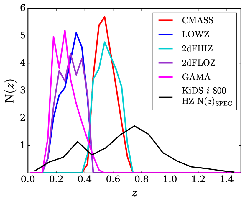
Figure 4: The redshift distributions for the five spectroscopic lens samples used in the analysis, plotted alongside the estimated redshift distribution of the KiDS-$i$-800 faint (HZ) sample, obtained using the overlap of deep spectroscopic redshifts described in Section 3.3.

3.2 The $r$-band redshift distribution

In KiDS-$r$-450, the multi-band observations allow us to determine a Bayesian point estimate of the photometric redshift, $z_{\rm B}$, for each galaxy using the photometric redshift code BPZ (Benítez, 2000). We use this information to select source galaxies that are most likely to be behind our ‘LZ’ and ‘HZ’ lens samples.

The redshift distribution for these $z_{\rm B}$ selected KiDS-$r$-450 source samples is calibrated with the weighting technique of Lima et al. (2008), named ‘DIR’. Here we match $r$-band selected $ugri$ VST observations with deep spectroscopic redshifts from the COSMOS field (Lilly et al., 2009), the Chandra Deep Field South (CDFS) (Vaccari et al., 2010) and two DEEP2 fields (Newman et al., 2013). This matched spectroscopic redshift catalogue is then re-weighted in multi-dimensional magnitude-space such that the weighted density of spectroscopic objects is as similar as possible to the lensfit-weighted density of the KiDS-$r$-450 lensing catalogue in each position in magnitude-space. It was shown in Hildebrandt et al. (2017) that this ‘DIR’ method produced reliable redshift distributions, with small bootstrap errors on the mean redshift, in the photometric redshift range $0.1<z_{\rm B}\leqslant 0.9$. As such, we adopt this DIR method and selection for our KiDS-$r$-450 galaxy-galaxy lensing analysis.

3.3 Estimating the $i$-band redshift distribution

To estimate a redshift distribution for KiDS-$i$-800 we choose not to adopt the ‘DIR’ method for a number of practical reasons. As discussed in Section 2.5, an $i$-band detected object catalogue differs from an $r$-band detected object catalogue, with $\sim 10$ percent of the $i$-band objects not present in the $r$-band catalogue. To create a weighted $i$-band spectroscopic sample would have required a full re-analysis of the VST imaging of the spectroscopic fields using the $i$-band imaging as the detection band. Furthermore, the DIR method was shown to be accurate in the photometric redshift range $0.1<z_{\rm{B}}\leqslant 0.9$ and as the majority of KiDS-$i$-800 only has single-band photometric information, it is not clear whether one can define a safe sample for which this method works reliably.

Our first estimate of the $i$-band redshift distribution, named ‘SPEC’, instead comes from using the COSMOS and CDFS spectroscopic catalogues directly as they are fairly complete at the relatively shallow magnitude limits of the KiDS-$i$-band imaging. In this case, we estimate the total redshift distribution, $N(z)$, by drawing a sample of spectroscopic galaxies such that their $i$-band magnitude distribution matches the lensfit weighted $i$-band magnitude distribution for all KiDS-$i$-800 galaxies. Given this methodology we do not include the DEEP2 catalogues used for the ‘DIR’ calibration of the $r$-band redshifts, as these have been colour-selected and therefore are not representative of the $i$-band magnitude limited sample. The resulting redshift distribution is shown in the left-hand panel of Figure 5, along with the average $r$-band DIR $N(z)$ with the $z_{\rm{B}}$ selection imposed. A bootstrap analysis determined the small statistical error in these redshift distributions and is illustrated by the thickness of the line. Any systematic error, due to sample variance or incompleteness in the spectroscopic catalogue, is not represented by the bootstrap error analysis.

As the KiDS-$i$-800 dataset lacks multi-band information and hence photometric redshift information per galaxy we choose to select galaxies based on their $i$-band magnitude to increase the average redshift of the source sample. Using our chosen bright magnitude limit of $i>19.4$ (see Section 2.3), the lensfit weighted source sample corresponds to a median redshift above $z_{\rm{med}}=0.43$. This magnitude selection is therefore suitable as a source sample for our ‘LZ’ lens analysis. Adopting a magnitude limit of $i>20.9$, we find that the faint $i$-band sample has a median redshift $z_{\rm{med}}=0.7$, thus making a suitable source sample for our ‘HZ’ lens sample (see Figure 15 in Appendix B for further details). The right-hand panel of Figure 5 shows the SPEC estimated redshift distributions for the KiDS-$i$-800 bright (LZ) and faint (HZ) source galaxy samples. The median redshifts of these samples are 0.50 and 0.57, respectively.

Figure 4 compares the predicted redshift distribution of the $i>20.8$ KiDS-$i$-800 HZ source sample with the redshift distributions of the lens samples. This demonstrates that even with the imposed magnitude cut on the KiDS-$i$-800 source galaxies, a significant fraction of source galaxies are still positioned in front of lenses thus diluting the signal. In the case of galaxy-galaxy lensing, uncertainty in the redshift distributions can therefore contribute significantly to the error budget and we seek to quantify this uncertainty by investigating two additional methods to estimate the KiDS-$i$-800 redshift distribution, using 30-band photometric redshifts (Section 3.4) and a cross-correlation technique (Section 3.5).

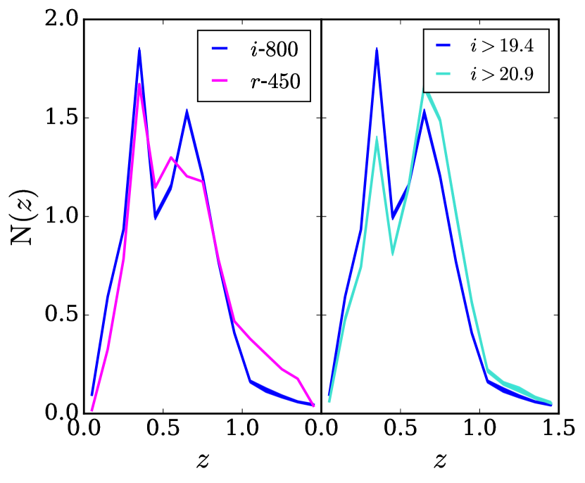
Figure 5: The estimated redshift distributions obtained using the overlapping spectroscopic data. Left: $N(z)$ for KiDS-$i$-800 (blue) estimated using the SPEC method, described in Section 3.3 and the KiDS-$r$-450 (pink) estimated via the DIR method. The median redshifts are comparable at 0.50 and 0.57, for KiDS-$i$-800 and KiDS-$r$-450 respectively. The sampling of the distribution is bootstrapped for an error, indicated by the thickness of the lines. Right: The estimated $N(z)$ for KiDS-$i$-800 for a brighter (blue) and fainter (cyan) magnitude limit.

3.4 Magnitude-weighted COSMOS-30 redshifts

One pointing in the KiDS-$r$-450 dataset overlaps with the well studied Hubble Space Telescope COSMOS field (Scoville et al., 2007). This field has been imaged using a combination of 30 broad, intermediate, and narrow photometric bands ranging from UV (GALEX) to mid-IR (Spitzer-IRAC), and this photometry has been used to determine accurate photometric redshifts (COSMOS-30 Ilbert et al., 2009; Laigle et al., 2016). Comparison with the spectroscopic zCOSMOS-bright sample shows that for $i<22.5$, the COSMOS-30 photometric redshift error $\sigma_{\Delta z/(1+z)}=0.007$. For the full sample with $z<1.25$, the estimates on photo-z accuracy are $\sigma_{\Delta z}=0.02,0.04,0.07$ for $i\sim 24.0$, $i\sim 25.0$, $i\sim 25.5$ respectively (Ilbert et al., 2009). As the COSMOS-30 photo-z catalogue is complete at the magnitude limits of KiDS-$i$-800, it provides a complementary estimate of the $i$-band redshift distribution.

We first match the multi-band KiDS-$r$-450 catalogue, in terms of both position and magnitude, with the COSMOS Advanced Camera for Surveys General Catalog (ACS-GC Griffith et al., 2012) which includes the 30-band photometric redshifts from Ilbert et al. (2009). These catalogues contain both stars and galaxies, which were labelled manually after the matching, by looking at the magnitude-size plot using the HST data where the separation was clean [see Hildebrandt et al. (in prep) for further details]. Once matched we sample the catalogue such that the $i$-band magnitude distribution of the selected COSMOS-30 galaxies matches the KiDS-$i$-800 lensfit weighted magnitude distribution. Similar to the case of using a spectroscopic reference catalogue, the bootstrap analysis of the resulting $i$-band redshift distribution shows a negligible statistical error.

3.5 Cross-correlation (CC)

The third redshift distribution estimate is constructed by measuring the angular clustering between the KiDS-$i$-800 photometric sample and the overlapping GAMA and SDSS spectroscopic samples. Clustering redshifts are based on the fact that galaxies in photometric and spectroscopic samples of overlapping redshift distributions reside in the same structures, thereby allowing for spatial cross-correlations to be used to estimate the degree to which the redshift distributions overlap and therefore, the unknown redshift distribution. Our approach is detailed in Schmidt et al. (2013) and Ménard et al. (2013) and further developed in Morrison et al. (2017), who describe the-wizz, the software we employ to estimate our redshifts from clustering. A similar clustering redshift technique was employed in Choi et al. (2016), Johnson et al. (2017) as well as Hildebrandt et al. (2017), but in the latter case the angular clustering was measured between the KiDS-$r$-450 galaxies and COSMOS and DEEP2 spectroscopic galaxies.

We exploit the overlapping lower-redshift SDSS and GAMA spectroscopy, the same surveys used in Morrison et al. (2017). The bulk of the spectroscopic sample is at a low redshift, limiting the redshift range that can be precisely constrained to $z<1.0$. This is because the high-redshift cross-correlations rely on the low density of spectroscopic quasars from SDSS. As the $i$-band galaxies comprise a shallower dataset than KiDS-$r$-450, these spectroscopic samples were deemed appropriate. The correlation functions are estimated over a fixed range of proper separation $100-1000\,\mathrm{kpc}$.

The amplitude of the redshift estimated from spatial cross-correlations is degenerate with galaxy bias. We employ a simple strategy to mitigate for this effect by splitting the unknown-redshift sample in order to narrow the redshift distribution a priori, in the absence of a photometric redshift estimate (Schmidt et al., 2013; Ménard et al., 2013; Rahman et al., 2016). This renders a more homogeneous unknown sample with a narrower redshift span, thereby minimising the effect of galaxy bias evolution as a function of redshift. As we have only the $i$-band magnitude available to us, a separation in redshift for this analysis would be imperfect. The KiDS-$i$-800 galaxies are divided by $i$-band magnitude into bins of width $\Delta i=0.5$ and the clustering redshift estimated for each subsample. The combination of these, with each subsample weighted by its number of galaxies, is shown in Figure 6. We conduct a bootstrap re-sampling analysis of the spectroscopic training set over the KiDS and GAMA overlapping area, where each sampled region is roughly the size of a KiDS pointing, for each magnitude subsample, in order to mitigate spatially-varying systematics in the cross-correlation. This revealed large statistical errors in the high-redshift tail of the distribution, represented by the large extent of the confidence contours in Figure 6. With the noisy high-redshift tail, it is possible for the cross-correlation method to produce negative, and therefore unphysical values in the full redshift distribution $N(z)$. In such cases, the final distribution is re-binned with a coarser redshift resolution in order to attain positive values in each redshift bin.

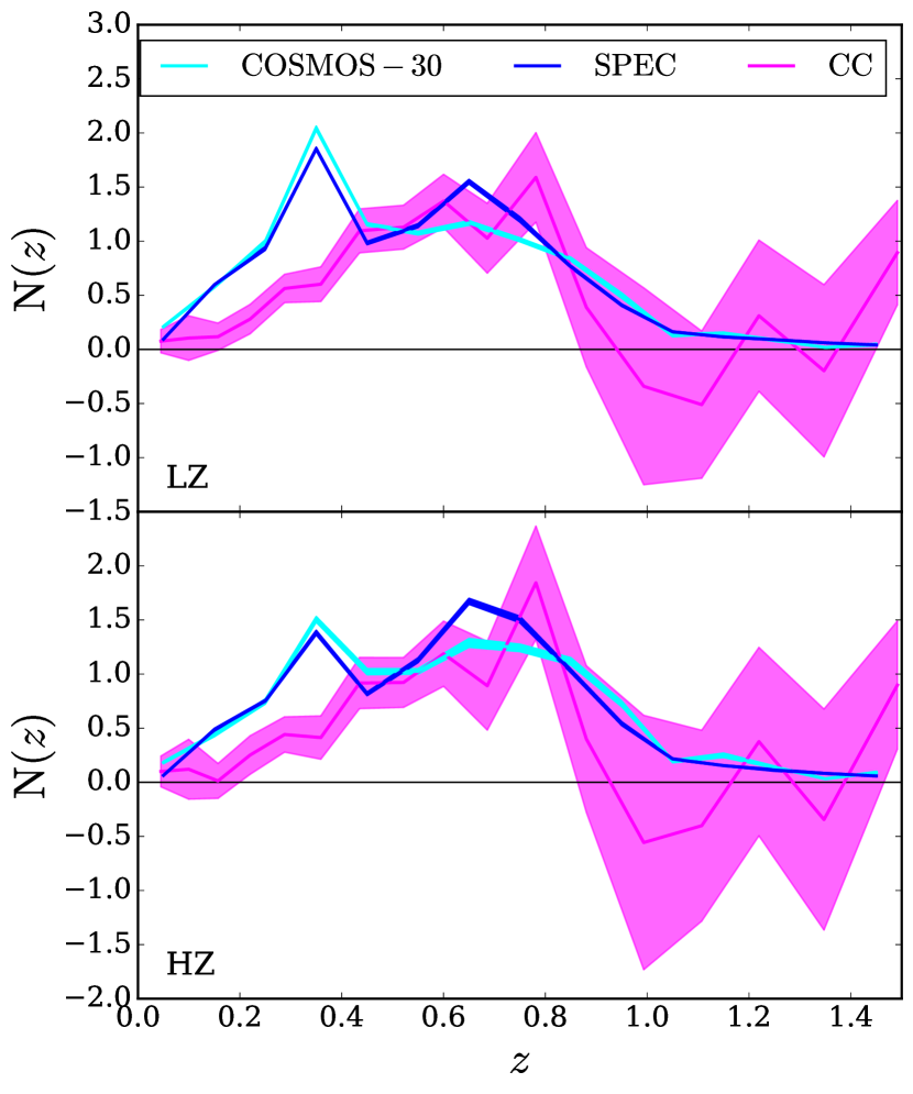
Figure 6: Comparison of the normalised redshift distributions for the LZ bright sample of KiDS-$i$-800 galaxies (upper panel) and the HZ faint sample (lower panel). The distributions shown are estimated using the spectroscopic catalogue (SPEC, Section 3.3 ), plotted in blue, the COSMOS-30 photometric redshift catalogue (COSMOS-30, Section 3.4) in cyan and from angular cross-correlations (CC, Section 3.5) in pink.

3.6 Comparison of $i$-band redshift distributions

Table 1: Values for the mean and median of the source redshift distributions, as well as the lensing efficiency, $\eta$. The redshift distribution for the KiDS-$r$-450 subsamples is estimated using the DIR method. For KiDS-$i$-800 galaxies, redshifts are estimated using overlapping, deep spectroscopic surveys (SPEC), the COSMOS photometric catalogue (COSMOS-30) and the cross-correlations method (CC). The quoted errors are determined from a bootstrap resampling.

Range	Dataset	Method	$z_{\rm{med}}$	$\bar{z}$	$\eta$
LZ	KiDS-$r$-450 ($0.1<z_{\rm{B}}<0.9$)	DIR	0.57	0.65	0.428
	KiDS-$i$-800 ($i>19.4$)	SPEC	$0.501\pm 0.002$	$0.555\pm 0.001$	0.361
		COSMOS-30	$0.452\pm 0.003$	$0.538\pm 0.002$	0.344
		CC	$0.6\pm 0.2$	$0.6\pm 0.2$	0.449
HZ	KiDS-$r$-450 ($0.43<z_{\rm{B}}<0.9$)	DIR	0.66	0.73	0.177
	KiDS-$i$-800 ($i>20.8$)	SPEC	$0.574\pm 0.002$	$0.607\pm 0.002$	0.126
		COSMOS-30	$0.545\pm 0.005$	$0.594\pm 0.003$	0.121
		CC	$0.6\pm 0.3$	$0.6\pm 0.2$	0.117

We illustrate the three estimated redshift distributions for the KiDS-$i$-800 HZ and LZ samples in Figure 6, and compare the mean and median redshifts for each estimate with that of KiDS-$r$-450 in Table 1. This table also includes an estimate of the lensing efficiency $\eta(z_{\rm l})$ for each estimated source redshift distribution, with

$$\eta(z_{\rm l})=\int^{\infty}_{z_{\rm l}}{\rm d}z_{\rm s}\,N(z_{\rm s})\left(\frac{\chi(z_{\rm l},z_{\rm s})}{\chi(z_{\rm s})}\right)\,,$$ (6)

where the source sample is characterised by a normalised redshift distribution $N(z_{\rm s})$ and $z_{\rm l}$ is set to 0.29 and 0.56 for the LZ and HZ case, respectively. Here the lensing efficiency, for a flat geometry Universe, scales with the comoving distances to the source galaxy, $\chi(z_{\rm s})$ and the comoving distance between the lens and the source $\chi(z_{\rm l},z_{\rm s})=\chi(z_{\rm s})-\chi(z_{\rm l})$.

As already seen in Figure 6, the different methods used to estimate the $i$-band redshifts result in quite different source redshift distributions. In Table 1 we see that the resulting mean and median redshift can differ by up to 15 percent, with the COSMOS-30 method favouring a shallower redshift distribution and the CC estimate generally preferring the deepest distribution. These differences are particularly pronounced for the low-redshift galaxy sample (with mean redshifts of 0.54 and 0.56 for the COSMOS-30 and SPEC methods and 0.6 for the CC technique). For galaxy-galaxy lensing studies, the impact of these differences in the estimated redshift distributions can be determined from the value of the lensing efficiency term $\eta$, in the final column of Table 1, which differs by up to 30 percent. This demonstrates the limitations of single-band imaging for weak lensing surveys and the importance of determining accurate source redshift distributions for weak lensing studies.

The drawback of using the SPEC method is that it is only a one-dimensional re-weighting of the magnitude-redshift relation. Section C3 of Hildebrandt et al. (2017) highlights the differences in the population in different colour spaces between the spectroscopic sample and the KiDS sample. As these differences are essentially unaccounted for in our SPEC method we expect that it could bias our estimation of the redshift distribution systematically. In contrast the COSMOS-30 catalogue provides a complete and representative sample for the KiDS-$i$-800 data, with the drawback that redshifts are photometrically estimated.

A drawback of both the COSMOS-30 method and the SPEC method, is that the calibration samples represent small patches in the Universe. COSMOS imaging spans $2\text{\,}{\mathrm{deg}}^{2}$ while the spectroscopic data, z-COSMOS and CDFS collectively, span roughly $1.2\text{\,}{\mathrm{deg}}^{2}$ with two independent lines-of-sight. We compute the variance between ten instances of randomly sub-sampling the $i$-band magnitude distribution from the SPEC or COSMOS-30 catalogue. This ‘bootstrap’ error analysis will not however include sampling variance errors. The resulting redshift distributions can be compared to the more representative $343\text{\,}{\mathrm{deg}}^{2}$ of homogenous spectroscopic data used in the cross-correlation technique. The depleted number density of galaxies with redshifts $0.2<z<0.4$ determined using the cross-correlation technique, in comparison to source redshift distributions determined using the SPEC and COSMOS-30 estimates, could be an indication that the SPEC and COSMOS-30 methods are subject to sampling variance in this redshift range.

Aside from suppressing sample variance, the cross-correlation method (CC) bypasses the need for a complete spectroscopic catalogue. On the other hand, however, the cross-correlation method (CC) is hindered by the impact of unknown galaxy bias, which tends to skew the clustering-redshifts to higher values if galaxy bias increases with redshift. One caveat of this method is that linear, deterministic galaxy bias may not apply on small scales. Our method to mitigate this effect using the $i$-band magnitude is reasonable given the level of accuracy required in this analysis, but for future studies this uncertainty will need to be addressed. In addition, the limited number of high-redshift objects in the spectroscopic catalogues that we have used makes it difficult for the clustering analysis to constrain the high-redshift tail of the distribution.

As there are pros and cons associated with each of the methods that we employ to determine the source redshift distribution, we present the galaxy-galaxy lensing analysis that follows using all three estimations. While we can constrain the statistical uncertainty of each of the estimates using our bootstrap analyses, we rely on the spread between the resulting lensing signals to reflect our systematic uncertainty in the $i$-band redshift distribution.

4 Comparison of i-band and r-band shape catalogues

We define the effective number density of galaxies following Heymans et al. (2012b), as

$$\centering n_{\mathrm{eff}}=\frac{1}{A}\frac{(\Sigma_{j}w_{j})^{2}}{\Sigma_{j}w_{j}^{2}}\,,\@add@centering$$ (7)

where $A$ is the total unmasked area and $w_{j}$ the lensfit weight for galaxy $j$. This definition gives the equivalent number density of unit-weight sources with a total ellipticity dispersion, per component, $\sigma_{\epsilon}$, that would create a shear measurement of the same precision as the weighted data. We define the observed ellipticity dispersion as,

$$\sigma_{\epsilon}^{2}=\frac{1}{2}\frac{\Sigma_{j}w_{j}^{2}\epsilon_{j}\bar{\epsilon}_{j}}{\Sigma_{j}w_{j}^{2}}\,,$$ (8)

where $\epsilon$ is the observed complex galaxy ellipticity (see equation 3). For KiDS-$i$-800 we find $n_{\rm eff}=3.80$ galaxies arcmin^-2 with an ellipticity dispersion of $\sigma_{\epsilon}=0.289$. This can be compared to KiDS-$r$-450 with $n_{\rm eff}=8.5$ galaxies arcmin^-2 and $\sigma_{\epsilon}=0.290$.

In Figure 7 we compare the effective number density, $n_{\mathrm{eff}}$, the ellipticity dispersion, $\sigma_{\epsilon}$, the median redshift and the percentage areal coverage to the observed $r$- and $i$-band seeing. The upper panel of Figure 7 shows that the KiDS-$i$-800 data have a lower effective number density than that of the KiDS-$r$-450 sample by a factor of roughly two over the full seeing range. This reflects the different depths of the KiDS $r$- and $i$-band observations. The second panel demonstrates that as the seeing in the $i$-band degrades, the observed ellipticity dispersion remains constant to a few percent. We see a very small effect of an increase in shape measurement noise ($\epsilon^{\rm n}$ in equation 5) as the fraction of galaxies with a size that is comparable with the PSF grows. Overall, we see that the total effective number of galaxies in each of the two datasets are roughly comparable with 10.0 million in KiDS-$i$-800 and 10.8 million in KiDS-$r$-450, after applying the photometric redshift limitations of $0.1<z_{\rm B}<0.9$. Therefore, the large-scale area of KiDS-$i$-800 still qualifies it as a competitive dataset.

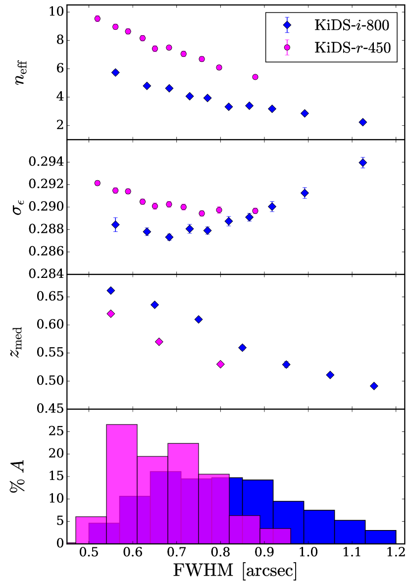
Figure 7: The variation of the effective number density, $n_{\mathrm{eff}}$, (measured in galaxies arcmin^-2), the observed ellipticity dispersion per component, $\sigma_{\epsilon}$, the median redshift of the estimated redshift distribution, $z_{\mathrm{med}}$ and the percentage area of the survey, $A$, with the seeing of the data. The KiDS-$r$-450 data is plotted in pink and the KiDS-$i$-800 in blue. Note that the KiDS-$r$-450 data has the high photometric redshift limit imposed at $z_{B}<0.9$. Error bars plotted for the upper three panels are the outcome of a bootstrap analysis.

Table 2: Number densities of weak lensing source galaxies drawn from KiDS (Kuijken et al., 2015; Hildebrandt et al., 2017), HSC (Mandelbaum et al., 2017), RCSLenS (Hildebrandt et al., 2016), CFHTLenS (Heymans et al., 2012b), DLS (Jee et al., 2013) and DES (Jarvis et al., 2016). The second column shows the effective area that the dataset spans in deg² (equation 7), although we note that the numbers quoted from DLS and HSC may have been defined differently in comparison to the other surveys in this table, the third shows the median FWHM seeing of the data, measured in arcsec, the fourth shows the weighted effective number density of galaxies arcmin^-2, the fifth column details the observed ellipticity dispersion per component and the sixth column shows the estimated median redshift of the galaxy sample. The DES measurements correspond to their primary shape measurement algorithm, NGMIX. The bracketed numbers for RCSLenS correspond to the reduced area where $griz$-band coverage exists, as opposed to their single-band dataset.

Sample	A [deg2]	FWHM [arcsec]	$n_{\rm{eff}}$ [galaxies arcmin-2]	$\sigma_{\epsilon}$	$z_{\rm{med}}$
DLS	20	0.88	$\sim$21.0		$\sim 1.0$
HSC Y1	137	0.58	21.8	0.24	$\sim 0.85$
DES SV	139	1.08	6.8	0.265	$\sim 0.65$
CFHTLenS	126	<0.8	15.1	0.280	0.7
RCSLenS	572(384)	<1.0	5.5(4.9)	0.251	$\sim 0.6$
KiDS-$r$-450	360	0.66	8.5	0.290	0.57
KiDS-$i$-800	733	0.79	3.8	0.289	$\sim 0.5$

Using the magnitude-weighted spectroscopic method (SPEC, Section 3.3) to estimate the $i$-band redshift distribution, we show, in the third panel of Figure 7, how the variable seeing KiDS-$i$-800 observations changes the depth of the sample of galaxies, with a higher median redshift for the better-seeing data. The same trend can be seen for the DIR $r$-band median redshift for three seeing samples, noting that a high photometric redshift limit of $z_{B}<0.9$ has been imposed for KiDS-$r$-450, lowering the overall median redshift in comparison to KiDS-$i$-800.

Finally, the lowest panel of Figure 7 presents the seeing distribution of the KiDS data, with the poorest seeing for KiDS-$r$-450 at a sub-arcsec level, while the KiDS-$i$-800 data extends to a FWHM of 1.2 arcsec. This figure illustrates that the KiDS-$i$-800 is a conglomerate of widely-varying quality data, in terms of seeing, and as a result, in terms of galaxy number density and depth. In Table 2 the survey parameters of KiDS-$i$-800 can be compared to other existing surveys: KiDS-$r$-450, HSC Y1, DES SV, RCSLenS, CFHTLenS and DLS. We order the surveys by their unmasked area and quote the median FWHM and median redshift of the data. We quote values for the number of galaxies arcmin^-2 using the definition given in equation 7 and the ellipticity dispersion as in equation 8.

To compare the shear measurement in KiDS-$i$-800 and KiDS-$r$-450, the most straightforward analysis would appear to be a direct galaxy-by-galaxy test (see for example Heymans et al., 2005). This would only be appropriate, however, if we had an unbiased shear measurement per galaxy. Even with perfect modelling and correction for the PSF, each shape catalogue consists of a noisy ellipticity estimate per galaxy, $\epsilon^{\rm n}$(equation 5). As ellipticity is a bounded quantity $|\epsilon|<1$, the presence of noise will always result in an overall reduction in the measured average galaxy ellipticity of a sample, an effect that has been termed ‘noise bias’ (Melchior & Viola, 2012). The impact of noise bias when using observed galaxy ellipticities as a shear estimate can be calibrated and accounted for (see for example Fenech Conti et al., 2017). This calibration correction, however, only applies when considering an ensemble of galaxies. A secondary issue for a galaxy-by-galaxy comparison of two catalogues from different filters arises from colour gradients in galaxies (Voigt et al., 2012). With a strong colour gradient, the intrinsic ellipticity of the object, when imaged in a blue filter, could be rather different from the intrinsic ellipticity of the same object when viewed in a red filter (see for example Schrabback et al., 2016). For these two reasons we do not perform any direct galaxy-by-galaxy comparisons, favouring instead tests where we should recover the same shear measurement from the ensemble of galaxies.

In this section we subject the $i$- and $r$-band shape catalogues to two different tests; a ‘nulled’ two-point shear correlation function which tests the difference in the shear recovered for a sample of galaxies with shape measurements in both bands, and a galaxy-galaxy lensing analysis which provides a joint-test of the shape and photometric redshift measurements for the full catalogue in each band.

4.1 The ‘nulled’ two-point shear correlation function

Using the matched $ri$ catalogue described in Section 2.5, we calculate the uncalibrated (the multiplicative calibrations are applied later to the ensemble) two-point shear correlation function, $\xi_{\pm}$, as a function of angular separation $\theta$, for three combinations of the $i$ and $r$-band filters, $({\rm fg})=(ii),(ir),(rr)$, with

$$\xi_{\pm}^{\rm fg}(\theta)=\frac{\Sigma w^{ir}(\mbox{\boldmath{$x_{a}$}})w^{ir}(\mbox{\boldmath{$x_{b}$}})[\epsilon_{\rm t}^{\rm f}(\mbox{\boldmath{$x_{a}$}})\epsilon_{\rm t}^{\rm g}(\mbox{\boldmath{$x_{b}$}})\pm\epsilon_{\times}^{\rm f}(\mbox{\boldmath{$x_{a}$}})\epsilon_{\times}^{\rm g}(\mbox{\boldmath{$x_{b}$}})]}{\Sigma w^{ir}(\mbox{\boldmath{$x_{a}$}})w^{ir}(\mbox{\boldmath{$x_{b}$}})}\,.$$ (9)

Here the weighted sum is taken over galaxy pairs with $|\mbox{\boldmath{$x_{a}$}}-\mbox{\boldmath{$x_{b}$}}|$ within the interval $\Delta\theta$ around $\theta$. The tangential and rotated ellipticity, $\epsilon_{\rm t}$ and $\epsilon_{\times}$, are determined via a tangential projection of the ellipticity components relative to the vector connecting each galaxy pair (Bartelmann & Schneider, 2001). For all filter combinations the weights, $w^{ir}=\sqrt{w_{i}w_{r}}$, use information from both the $i$ and $r$-band analyses such that the effective redshift distribution of the matched sample is identical for each measurement.

We calculate empirically any additive bias terms for our matched $ri$ catalogues using $c_{i}=\langle\epsilon_{i}\rangle$, where the average now takes into account the combined weight $w^{ir}$. We apply this calibration correction to both the $i$ and $r$-band shapes, per patch on the sky, in the matched catalogue where on average, $c_{1}^{r}=0.0001\pm 0.0001$, $c_{2}^{r}=0.0008\pm 0.0001$, $c_{1}^{i}=0.0009\pm 0.0001$, $c_{2}^{i}=0.0010\pm 0.0001$. This level of additive bias is similar to that of the full KiDS-$i$-800 and KiDS-$r$-450 samples.

Following Miller et al. (2013), the ensemble ‘noise bias’ calibration correction for each filter combination is given by

$$1+{\rm K}^{\rm fg}(\theta)=\frac{\Sigma w^{ir}(\mbox{\boldmath{$x_{a}$}})w^{ir}(\mbox{\boldmath{$x_{b}$}})[1+m^{\rm f}(\mbox{\boldmath{$x_{a}$}})][1+m^{\rm g}(\mbox{\boldmath{$x_{b}$}})]}{\Sigma w^{ir}(\mbox{\boldmath{$x_{a}$}})w^{ir}(\mbox{\boldmath{$x_{b}$}})}\,,$$ (10)

where $m^{f}(\mbox{\boldmath{$x_{a}$}})$ is the multiplicative correction for the galaxy at position $(\mbox{\boldmath{$x_{a}$}})$ imaged with filter $f$. These multiplicative corrections are calibrated as a function of signal-to-noise and relative galaxy-to-PSF size using image simulations (Fenech Conti et al., 2017). For this matched $ri$ sample the Fenech Conti et al. (2017) calibration corrections are found to be small and independent of scale, with $1+{\rm K}^{rr}=0.996$, $1+{\rm K}^{ir}=0.987$ and $1+{\rm K}^{ii}=0.978$.

We define two ‘nulled’ two-point shear correlation functions as

$$\xi_{\pm}^{\rm null}(\theta)=\frac{\xi_{\pm}^{ii}(\theta)}{1+{\rm K}^{ii}(\theta)}-\frac{\xi_{\pm}^{rr}(\theta)}{1+{\rm K}^{rr}(\theta)}\,,$$ (11)

$$\xi_{\pm}^{\rm x-null}(\theta)=\frac{\xi_{\pm}^{ir}(\theta)}{1+{\rm K}^{ir}(\theta)}-\frac{\xi_{\pm}^{rr}(\theta)}{1+{\rm K}^{rr}(\theta)}\,,$$ (12)

which, for a matched catalogue in the absence of unaccounted sources of systematic error, would be consistent with zero. The three different matched-catalogue measurements of $\xi_{\pm}^{\rm fg}$ will be subject to the same cosmological sampling variance error. The covariance matrix for our ‘nulled’ two-point statistics therefore, derives only from noise on the shape measurement in addition to noise arising from differences in the source intrinsic ellipticity when imaged in the $r$- or $i$-band (see Appendix E). As such the covariance is only non-zero on the diagonal and given by

$$C^{\rm null}_{\xi}(\theta_{j},\theta_{j})=\frac{4}{N_{\rm p}(\theta_{j})}(\sigma^{4}_{i}+\sigma^{4}_{r}-2\sigma^{4}_{\rm int})\,,$$ (13)

$$C^{\rm x-null}_{\xi}(\theta_{j},\theta_{j})=\frac{2}{N_{\rm p}(\theta_{j})}[2\sigma^{4}_{r}+\sigma^{4}_{\rm int}+\sigma^{2}_{r}(\sigma^{2}_{i}-4\sigma^{2}_{\rm int})]\,.$$ (14)

Here $\sigma_{i}^{2}$ and $\sigma_{r}^{2}$ are the measured weighted ellipticity variance, per component (as defined in equation 8), of the matched catalogue in the $i$- and $r$-band, respectively. For a single ellipticity component, $\sigma^{2}_{\rm int}$ is the variance of the part of the intrinsic ellipticity distribution that is correlated between the $i$- and the $r$-band and $N_{\rm p}(\theta)$ counts the number of pairs in each angular bin which is given by

$$N_{\rm p}(\theta)=\pi(\theta_{u}^{2}-\theta_{l}^{2})A\,n_{\rm eff}^{2}\,.$$ (15)

Here $n_{\rm eff}$ is the effective number density as given in equation 7, $\theta_{u}$ and $\theta_{l}$ are the angular scales of the upper and lower bin boundaries and $A$ is the effective survey area (Schneider et al., 2002, see also Appendix E). For the $ri$ matched catalogue, we measure $\sigma_{i}=0.296$, $\sigma_{r}=0.265$, $n_{\rm eff}=3.64$ arcmin^-2 and we make an educated guess for $\sigma_{\rm int}=0.255$, based on SDSS measurements of the low-redshift intrinsic ellipticity distribution (see the discussion in Miller et al., 2013; Chang et al., 2013; Kuijken et al., 2015). Note that we choose not to include the uncertainty in the additive or multiplicative calibration corrections from equation 10 into our analytical error estimate for the nulled shear correlation functions, as this is smaller than our uncertainty on the value of the intrinsic ellipticity distribution $\sigma_{\rm int}$.

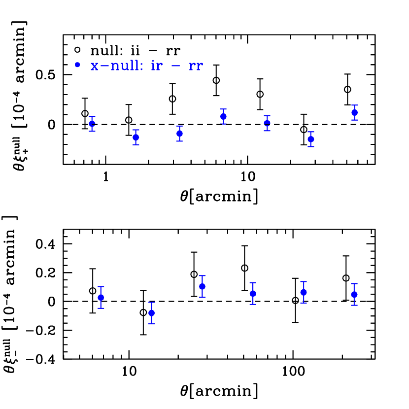
Figure 8: The ‘nulled’ two-point shear correlation functions $\xi_{\pm}^{\rm null}$ (open) and $\xi_{\pm}^{\rm x-null}$ (closed). Both the upper panel, $\xi_{+}$, and the lower panel, $\xi_{-}$, are scaled by $\theta$ to highlight any differences from zero on large scales.

Figure 8 presents measurements of $\xi_{\pm}^{\rm null}$ and $\xi_{\pm}^{\rm x-null}$. In the upper panel of Figure 8 we find $\xi_{+}^{\rm null}$ to be significantly different from zero on scales $\theta>$ $2\text{\,}\mathrm{arcmin}$. Defining $\chi^{2}_{\rm null}$ as

$$\chi^{2}_{\rm null}=\sum_{i}\frac{\xi^{\rm null}_{\pm}(\theta_{i})^{2}}{C^{\rm null}_{\xi}(\theta_{i},\theta_{i})}\,,$$ (16)

we find the ‘nulled’ two point shear correlation function to be inconsistent with zero with 99 percent probability ($\chi^{2}_{\rm null}=26.2$ for $13$ data points). These results allow us to conclude that unaccounted sources of systematics exist, which have a scale dependence; this is not surprising given the non-zero PSF contamination ($\alpha$), described in Section 2.4. This null-test therefore supports our conclusion that KiDS-$i$-800 is not suitable for cosmic shear studies. Interestingly these systematics appear to contribute roughly equally to tangential and rotated correlations, such that they approximately null themselves in the $\xi_{-}$ statistic in the lower panel of Figure 8. Limiting the $\chi^{2}_{\rm null}$ calculation to only the $\xi^{\rm null}_{-}$ measurements we find that $\xi^{\rm null}_{-}$ is consistent with zero with $\chi^{2}_{\rm null}=5.3$ for $6$ data points.

We define $\chi^{2}_{\rm x-null}$ by replacing the ‘nulled’ two point shear correlation function with the ‘cross-null’ statistic $\xi_{\pm}^{\rm x-null}$ in equation 16. We find $\xi_{\pm}^{\rm x-null}$ to be consistent with zero with 16 percent probability ($\chi^{2}_{\rm x-null}=16.8$ for $13$ data points). It has an average value over angular scales, using inverse variance weights, of $\langle\xi_{\pm}^{\rm x-null}\rangle=(3.9\pm 3.0)\times 10^{-8}$. From this we can conclude that the unaccounted sources of systematics highlighted by the $\xi_{\pm}^{\rm null}$ statistic are uncorrelated with the $r$-band catalogue. Importantly, finding a null result with this ‘cross-null’ statistic demonstrates that the multiplicative shear calibration corrections for the $i$ and $r$ catalogues in equation 10 produce consistent results. The inverse variance weighted average value of $\langle\xi_{\pm}^{\rm x-null}/\xi_{\pm}^{\rm rr}\rangle=0.010\pm 0.035$. In this ‘cross-null’ analysis that isolates the impact of multiplicative shear bias, the amplitude of the shear correlation functions for the matched $r$ and $i$ catalogues therefore agree at the level of $1\pm 4$ percent.

In this analysis we used the KiDS-$r$-450 auto-correlation function $\xi^{rr}_{\pm}$ as the ‘truth’ in the ‘cross-null’ statistic of equation 12. Given the significant KiDS-$i$-800 PSF residuals uncovered in Section 2.4 this was a sensible choice to make. In future cases, however, where both surveys have demonstrated low-levels of additive bias before the comparison analysis, the ‘cross-null’ statistic should be defined using both auto-correlations. This ‘cross-null’ test can then be used as a diagnostic to isolate which survey is the most trustworthy, in the event that the initial ‘null’ test of equation 11 has failed.

In the example where a ‘cross-nulled’ $ir-rr$ signal is consistent with zero, but the companion ‘cross-nulled’ $ir-ii$ signal is significant, we can conclude that unaccounted additive sources of systematics exist in the $i$-survey, which are uncorrelated with the $r$-survey.

In the example where both ‘cross-nulled’ signals are significant, the angular scale-dependence of these null-statistics can be analysed in order to distinguish between additive bias, which usually becomes significant on large scales, and multiplicative bias, which impacts all scales equivalently.

The ‘nulled’ two-point statistics defined in this section differ from the ‘differential shear correlation’ proposed by Jarvis et al. (2016). The differential statistic derives from a galaxy-by-galaxy comparison of the ellipticities in contrast to our chosen statistic which compares the calibrated ensemble averaged shear. We would argue that the Jarvis et al. (2016) approach is only appropriate when one is able to determine an unbiased shear measurement per galaxy. Our methodology also differs from the ‘split’ cosmic shear analyses conducted in Becker et al. (2016) and Troxel et al. (2017). Here the source sample is divided into groups based on a number of observational properties such as seeing, PSF ellipticity, sky brightness and observed object size and signal-to-noise. These groupings change the effective redshift distribution of each sample and introduce object selection bias (see for example Fenech Conti et al., 2017), adding an extra layer of complexity when interpreting the results of this split-analysis. If these changes can be accurately modelled, however, the ‘split’ cosmic shear analyses can provide a powerful tool to investigate the dependence of different systematic biases on a range of observational properties. Our approach of matching catalogues before conducting our ‘null’ cosmic shear tests removes this layer of complexity.

Finally we note the reduced uncertainties for the ‘cross-null’ two-point statistic in comparison to the ‘null’ statistic, in addition to the reduction of systematic errors. These two features of this multi-band cosmic shear analysis supports the Jarvis & Jain (2008) proposal to combine shear information from multiple filters to gain in effective number density, particularly if there are unknown, but uncorrelated systematic errors in each band. This idea will be explored further in future work.

4.2 Galaxy-galaxy Lensing Signal

Statistically, galaxy-galaxy lensing can be viewed as a 2-D measurement of the cross-correlation, $\xi_{\rm gm}$, of a baryonic tracer, such as a galaxy, as a relative overdensity with the fractional overdensity in the matter density field, separated by a comoving separation in 3-D space, ${\bf r}$, expressed as,

$$\xi_{\rm gm}({\bf r})=\langle\delta_{\rm g}({\bf x})\delta_{\rm m}({\bf x}+{\bf r})\rangle_{\rm{\bf x}}\,.$$ (17)

For a given cosmology, the relative amplitude of the galaxy-galaxy signals from different source samples will reflect their redshift distribution and any shear calibration systematics. As such, this measurement is commonly used to test the redshift scaling of weak lensing shear measurements (Hoekstra et al., 2005; Mandelbaum et al., 2005; Heymans et al., 2012b; Kuijken et al., 2015; Schneider, 2016; Hildebrandt et al., 2017). In this section we compare measurements of the galaxy-galaxy lensing signal from KiDS-$i$-800 and KiDS-$r$-450 using a common set of lens samples from GAMA, BOSS and 2dFLenS, as described in Section 3.1. This comparison provides an opportunity to assess the impact of using the different estimations of the $i$-band redshift distributions from Section 3 and the shear calibration, $m$, of the variable seeing KiDS-$i$-800 background galaxies, in comparison to the same measurement using KiDS-$r$-450 shapes.

4.2.1 Theory

The galaxy-galaxy lensing cross-correlation, $\xi_{\rm gm}(\bf{r})$ can be related to the comoving projected surface mass density around galaxies, $\Sigma$ with a comoving projected separation, $R$, as

$$\Sigma(R)=\rho_{\rm m,0}\int_{0}^{\chi(z_{\rm s})}\ \xi_{\rm gm}\big{(}\sqrt{R^{2}+[\chi-\chi(z_{\rm l})]^{2}}\big{)}\ \rm{d}\chi\,,$$ (18)

where $\chi(z_{\rm l}),\chi(z_{\rm s})$ are the comoving distances to the lens and source galaxies, respectively, $\rho_{\rm m,0}$ is the matter density of the Universe today and $\chi$ is the comoving line-of-sight separation. The shear is a measurement of the over-density in the matter distribution, therefore, it is a measure of the excess or differential surface density (Mandelbaum et al., 2005),

$$\Delta\Sigma(R)=\overline{\Sigma}(\leq R)-\Sigma(R)\,,$$ (19)

where

$$\overline{\Sigma}(\leq R)=\frac{2}{R^{2}}\int^{R}_{0}\Sigma(R^{\prime})R^{\prime}\rm{d}R^{\prime}\,.$$ (20)

The comoving differential surface mass density can be related to the tangential shear distortion $\gamma_{\rm t}$ of the background sources as

$$\Delta\Sigma(R)=\gamma_{\rm t}\Sigma_{c}\,,$$ (21)

in terms of a geometrical factor that accounts for the lensing efficiency, the comoving critical surface mass density, which is defined as

$$\Sigma_{c}=\frac{c^{2}}{4\pi G}\frac{\chi(z_{\rm s})}{\chi(z_{\rm l})\,\chi(z_{\rm l},z_{\rm s})\,(1+z_{\rm l})}\,,$$ (22)

where $z_{\rm l}$ is the redshift of the lens, $\chi(z_{\rm l})$ is the comoving radial co-ordinate of the lens at redshift $z_{\rm l}$, $\chi(z_{\rm s})$ is that of the source at redshift $z_{\rm s}$ and $\chi(z_{\rm l},z_{\rm s})$ is the comoving distance between the source and the lens. Comoving separations are determined assuming a flat $\Lambda$CDM cosmology with a Hubble parameter of $H_{0}=100\,h\,\rm{km\,Mpc^{-1}\,s^{-1}}$, fixing the matter density to $\Omega_{\rm m}=0.277$ (Komatsu et al., 2011). Given our statistical power, the galaxy-galaxy lensing measurements are fairly insensitive to the choice of fiducial cosmology, and as such, using a Planck Collaboration et al. (2016) cosmology would not significantly impact our analysis.

4.2.2 Estimators

The azimuthal average of the tangential ellipticity of a large number of galaxies in the same area of the sky is an unbiased estimate of the shear, in the absence of systematics. Following this, the galaxy-galaxy lensing estimator is calculated as a function of angular separation, $\theta$, as the weighted sum of the tangential ellipticity of the source-lens pairs, $\epsilon_{\rm t}$ as,

$$\gamma_{\rm t}(\theta)=\frac{\sum^{\rm N_{pairs}}_{jk}w_{\rm s}^{j}w_{\rm l}^{k}\epsilon_{\rm t}^{jk}}{\sum^{\rm N_{pairs}}_{jk}w_{\rm s}^{j}w_{\rm l}^{k}}\,,$$ (23)

where $w_{\rm s}$ are the lensfit weights of the sources and $w_{\rm l}$ are the weights of the lenses. For this measurement we employ the athena software of Kilbinger et al. (2014).

The estimator for the excess surface mass density is defined as a function of the projected radius, $R$, from the lens and the spectroscopic redshift of the lens, $z_{\rm l}$, in terms of the inverse critical surface mass density,

$$\overline{\Delta\Sigma}(R,z_{\rm l})=\frac{\gamma_{\rm t}(R/\chi_{\rm l})}{\overline{\Sigma_{c}^{-1}}(z_{\rm l})}\,.$$ (24)

Lens galaxy samples are split by their spectroscopic redshifts into finely defined ‘slices’ of width $\Delta z_{\rm l}=0.01$ and the inverse critical surface mass density is calculated per source-lens slice as,

$$\overline{\Sigma_{c}^{-1}}(z_{\rm l})=\frac{4\pi G}{c^{2}}\,(1+z_{\rm l})\,\chi(z_{\rm l})\,\eta(z_{\rm l})\,,$$ (25)

where $\eta(z_{\rm l})$, the lensing efficiency, is defined in equation 6. This geometric term accounts for the dilution in the lensing signal caused by the non-zero probability that a source is situated in front of the lens (Miyatake et al., 2015a; Blake et al., 2016a). It is computed for each lens using its spectroscopic redshift with the entire normalised source redshift probability distribution, $N(z)$. The tangential shear was measured in 7 logarithmic angular bins where the minimum and maximum $\theta$ angles were determined for each lens redshift via $R=\theta\,\chi(z_{\rm l})$, in order to satisfy a minimum and maximum comoving radii of $R=0.05$ and $R=2\,h^{-1}$Mpc.

For the case of KiDS-$r$-450, with the availability of the $z_{\rm B}$ photometric redshift information per galaxy, the source sample could be further limited to those behind each lens slice, in order to minimise the dilution of the lensing signal due to sources correlated with the lens. The stringency of this source redshift selection is investigated in Appendix D and a limit of $z_{\rm B}>z_{\rm l}+0.1$, is deemed optimal. We calculate the tangential shear and the differential surface mass density, $\Delta\Sigma(R)$, for each of the $N$ lens slices and stack these signals to obtain an average differential surface mass density, weighted by the number of pairs in each slice as,

$$\centering\overline{\Delta\Sigma}(R)=\frac{\sum^{N}_{i}(\gamma_{\rm t}(R/\chi_{\rm l})/\overline{\Sigma_{c}^{-1}})^{i}n_{\rm{pairs}}^{i}}{\sum^{N}_{i}n_{\rm{pairs}}^{i}}\frac{1}{1+K}\,,\@add@centering$$ (26)

where

$$\centering K=\frac{\sum_{\rm s}w_{\rm s}m_{\rm s}}{\sum_{\rm s}w_{\rm s}}\,.\@add@centering$$ (27)

This factor accounts for the multiplicative noise bias determined for each source galaxy, $m_{\rm s}$, weighted by its lensfit weight $w_{\rm s}$. Note that we assume that there is no significant dependence of the multiplicative calibration on the source redshift and therefore $\overline{\Sigma_{c}^{-1}}$. This was deemed suitable as this calibration is at the percent level for the ensemble.

Two corrections were made to the galaxy-galaxy lensing signal. Firstly, the excess surface mass density was computed around random points in the areal overlap. Random catalogues were generated following the angular selection function of the spectroscopic surveys, where we used a random sample 40 times bigger than the data sample. This signal has an expectation value of zero in the absence of systematics. As demonstrated by Singh et al. (2016), it is important that a random signal, $\Delta\Sigma_{\rm{rand}}(R)$, is subtracted from the measurement in order to account for any small but non-negligible coherent additive bias of the galaxy shapes and to decrease large-scale sampling variance. The random signals determined for both KiDS-$i$-800 and KiDS-$r$-450 were found to be consistent with zero for each lens sample. We present the random signals for each lens sample in Appendix D.

Secondly, as the estimates of the redshift distributions of the source galaxies have an associated level of uncertainty, it is necessary to account for the contamination of the clustering of source galaxies with the lens galaxies. Any sources that are physically associated with the lenses would not themselves be lensed and would therefore bias the lensing signal low at small transverse separations. To correct for this, we determine the ‘boost factor’ for each lens-source sample and amplify the excess surface mass density measurement by it, multiplicatively. We investigate the implication of redshift cuts on this factor in Appendix D. We assume that the boost signal originates from source-lens clustering and ignore any contribution from weak lensing magnification, which can also alter the number of sources behind the lens, as Schrabback et al. (2016) showed that this is only a small net effect. The overdensity of source galaxies around the lenses is estimated as the ratio of the weighted number of source-lens galaxy pairs for real lenses to that of the same number of randomly positioned lenses (again, where the weights and the redshift distribution of the lens sample is preserved), following Mandelbaum et al. (2006) as,

$$\centering B(R)=\frac{\sum^{\rm N_{pairs}}_{jk}w_{\rm s}^{j}w_{\rm l}^{k}}{\sum^{\rm N_{pairs}}_{jk}w_{\rm s}^{j}w_{\rm l}^{k}({\rm rand)}}\,.\@add@centering$$ (28)

This prescription is determined for each lens slice and the average boost, $\overline{B}(R)$ computed, weighted by the number of source-lens pairs in each slice. Hence, the corrected excess surface mass density is measured as,

$$\centering\overline{\Delta\Sigma}_{\rm{corr}}(R)=[\overline{\Delta\Sigma}(R)-\Delta\Sigma_{\rm{rand}}(R)]\,\overline{B}(R)\,.\@add@centering$$ (29)

We present the boost factors that we apply to each measurement in Appendix D.

4.2.3 Results

Figure 9 compares the KiDS-$i$-800 galaxy-galaxy lensing measurements, with the KiDS-$r$-450 measurement, for the five lens samples detailed in Section 3.1. KiDS-$i$-800 measurements are made using each of the three estimated redshift distributions described in Sections 3.3, 3.4 and 3.5. The error bars are estimated using a Jackknife technique, where each Jackknife sample estimate is obtained by removing a single KiDS-$i$-800 pointing, such that the number of estimates corresponds to the number of pointings with a spectroscopic overlap. The signals were measured for projected separations of 0.05 $h^{-1}\rm{Mpc}$ up to 2.0 $h^{-1}\rm{Mpc}$, limited by the size of the Jackknife sample following Singh et al. (2016). For the two high-redshift lens samples, CMASS and 2dFHIZ, we only consider scales of $R>0.08\,h^{-1}\rm{Mpc}$ as for our high-redshift lens sample, the projected separation $0.08\,h^{-1}\rm{Mpc}$ corresponds to an angular size smaller than the size of the lensfit galaxy shape measurement postage stamp (Miller et al., 2013).

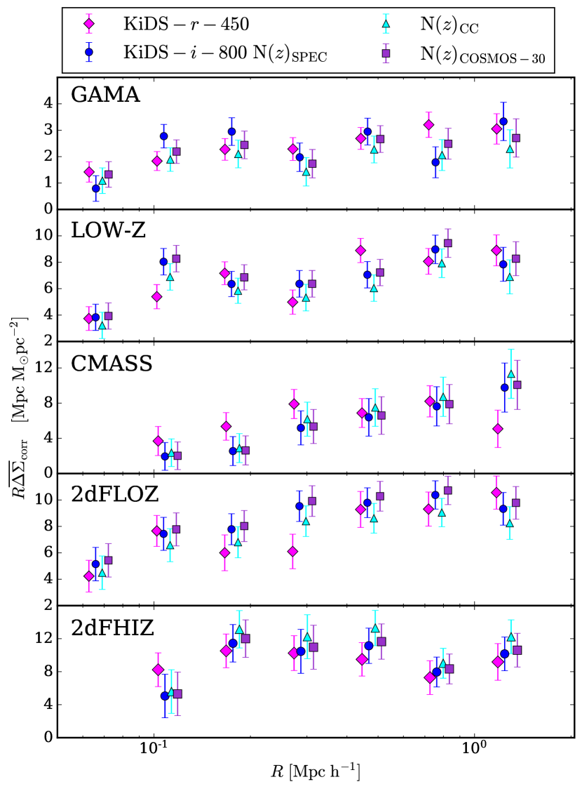
Figure 9: The stacked differential surface mass density measurements $\overline{\Delta\Sigma}_{\rm{corr}}(R)$ for KiDS-$i$-800 (blue) and KiDS-$r$-450 (pink) galaxies with GAMA, LOWZ, CMASS, 2dFLOZ and 2dFHIZ lens galaxy samples, from top to bottom. Three KiDS-$i$-800 signals are shown- one for each of the three redshift distributions. Jack-knifed errors are determined and plotted in combination with the random signal error. Note that the errors here do not include our uncertainty on the redshift distributions. Random signals have been subtracted and measurements have had ‘boost’ correction applied. In order to distinguish between the measurements on large-scales, all signals are scaled by $R$ and data points are offset on the $R$-axis for clarity.

As expected we see that the signal from the GAMA galaxies has the lowest amplitude as this lens sample is entirely magnitude limited, whereas the BOSS and 2dFLenS galaxies are samples of Luminous Red Galaxies (LRGs). A magnitude-limited sample includes galaxies of a lower luminosity or higher number density. These galaxies have a correspondingly lower bias factor and give rise to a lower amplitude lensing signal than the LRGs which tend to live in more massive halos. The 2dFLenS signals are higher than the BOSS counterparts as this luminosity-selected sample has a lower number density than BOSS and so preferentially selects dark matter halos of higher mass and hence a higher bias factor.

Figure 10 shows the inverse variance-weighted average fractional difference over all scales, $\langle\varphi\rangle$, between the KiDS-$i$-800 and KiDS-$r$-450 galaxy-galaxy lensing measurements, for each lens sample where

$$\varphi(R)=\frac{\overline{\Delta\Sigma}^{i}_{\rm{corr}}(R)-\overline{\Delta\Sigma}^{r}_{\rm{corr}}(R)}{\overline{\Delta\Sigma}^{r}_{\rm{corr}}(R)}\,,$$ (30)

with associated variance

$$\sigma^{2}_{\varphi}(R)=\frac{\overline{\Delta\Sigma}^{i}_{\rm{corr}}(R)^{2}}{\overline{\Delta\Sigma}^{r}_{\rm{corr}}(R)^{2}}\left(\frac{\sigma^{2}_{\overline{\Delta\Sigma}^{i}(R)}}{{\overline{\Delta\Sigma}^{i}_{\rm{corr}}}(R)^{2}}+\frac{\sigma^{2}_{\overline{\Delta\Sigma}^{r}(R)}}{{\overline{\Delta\Sigma}^{r}_{\rm{corr}}}(R)^{2}}\right)\,.$$ (31)

Here $\sigma^{2}_{\overline{\Delta\Sigma}}(R)$ is the error on the measurement of $\overline{\Delta\Sigma}_{\rm{corr}}(R)$ which is estimated using a Jackknife analysis. For the purposes of this comparison we make the approximation that radial bins are uncorrelated, which is a reasonable approximation to make for scales $R<1\,h^{-1}\,{\rm Mpc}$ (see Figure 5 in Viola et al., 2015). We also ignore the covariance between the KiDS-$i$-800 and KiDS-$r$-450 measurements which is appropriate given that the errors are dominated by intrinsic and measured ellipticity noise. Furthermore, the $i$ and $r$-band catalogues contain at most 40 percent of the same source galaxies in the case of our GAMA analysis, where the entire area analysed has overlapping KiDS-$i$-800 and KiDS-$r$-450 data and these overlapping galaxies have different weights in the different datasets (see Section 2.5). Typically the overlap of source galaxies is significantly less than this given the different on-sky distribution of the two surveys. We present an inverse variance-weighted average over all angular scales as there is little angular dependence in the measured fractional difference $\varphi(R)$.

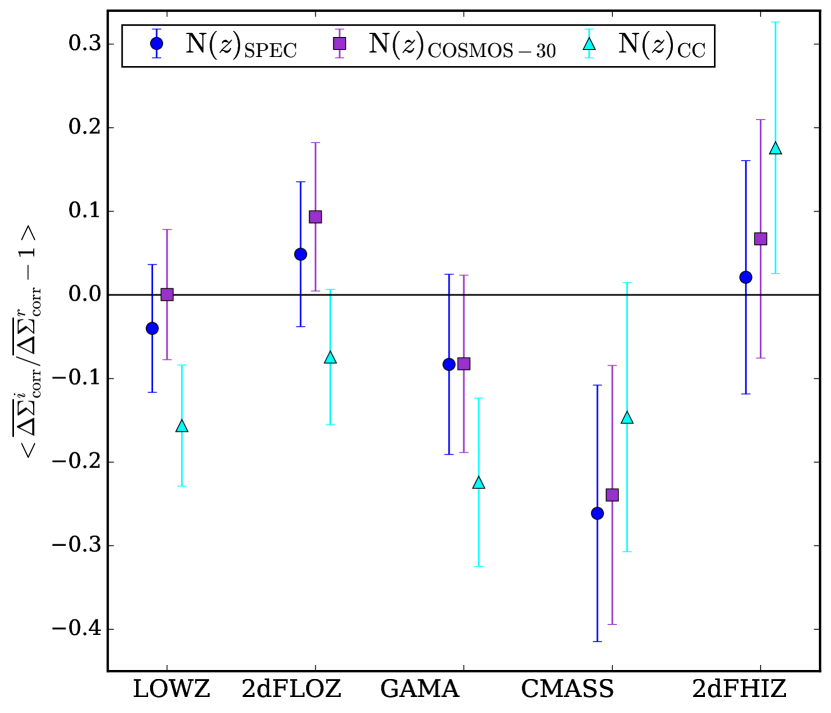
Figure 10: The average fractional difference between the KiDS-$i$-800 and KiDS-$r$-450 galaxy-galaxy lensing measurements, $\langle\varphi\rangle$ (an inverse variance-weighted combination of equation 30 over all scales), for each spectroscopic lens dataset using three different methods to estimate the redshift distribution of the $i$-band source galaxies. These measurements are inverse variance-weighted and do not include any uncertainty on the redshift distribution.

Figure 10 shows that for each of the low-redshift lens samples, LOWZ, 2dFLOZ and GAMA, using the three different redshift distributions results in KiDS-$i$-800 measurements that are consistent with each other and with that of KiDS-$r$-450. For CMASS and 2dFHIZ, the scatter between the three KiDS-$i$-800 measurements is larger, because these high-redshift lens samples are more sensitive to the tail of the source redshift distribution, which differs the most between each redshift estimation method. For these HZ lens samples, the measurement derived using both the SPEC and COSMOS-30 redshift distributions deviated the least from KiDS-$r$-450. As discussed in Section 3.6, the SPEC method, as a 1-D DIR method, is biased in comparison to the full DIR analysis in Hildebrandt et al. (2017), as it cannot take into account the difference in population of colour space between the KiDS sample and the deep spectroscopic samples. On the other hand, the spectroscopic sample employed in the cross-correlation redshift estimation method has a limited selection of high-redshift objects and therefore little constraining power at $z>1$.

Averaging over all lens samples and assuming independent measurements, both the COSMOS-30 and SPEC KiDS-$i$-800 measurements are found to be consistent with the KiDS-$r$-450 measurement at the level of $7\pm 5$%. For the low-redshift lens samples only, the results are consistent at the level of $5\pm 5$%. The KiDS-$i$-800 measurements using the cross-correlation redshift estimation (CC), are, on average, inconsistent with the KiDS-$r$-450 measurements. Combining all lens samples together we find that the KiDS-$i$-800 and KiDS-$r$-450 analyses differ by $14\pm 4$% for the CC analysis.

In this comparison we note that we have not accounted for the uncertainty in the estimate of each redshift distribution. For the cross-correlation (CC) result, in particular, the errors are significant at high redshift (see Figure 6) and this hinders the method from constraining the high-redshift tail. It is therefore unsurprising that this method nominally has the worst agreement as these significant errors have not been accounted for in this analysis. For the SPEC and COSMOS-30 redshift distributions, the bootstrap error is negligible but we have not been able to quantify likely systematic errors associated with sampling variance and incompleteness. The spread of the galaxy-galaxy lensing measurements for each lens sample therefore provides some indication of the impact on our analysis of our systematic uncertainty in the $i$-band source redshift distribution.

We find that our measurements of the excess surface mass density profiles are not only consistent between KiDS-$i$-800 and KiDS-$r$-450, but also with previous measurements, namely Miyatake et al. (2015b); Leauthaud et al. (2017); van Uitert et al. (2016). While the purpose of this study is to compare the two source galaxy datasets, these KiDS-$r$-450 measurements are interesting in their own right (Amon et al., 2017).

4.3 PSF and seeing dependence

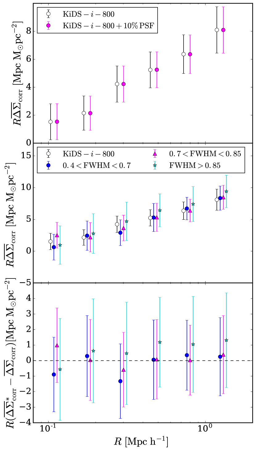
Figure 11: Stress-testing the galaxy-galaxy lensing measurement: the dependence of PSF contamination and seeing on the observed stacked differential surface mass density $\Delta\Sigma$ for KiDS-$i$-800 with CMASS lenses. The upper panel compares the lensing signal obtained with a false additional 10% PSF contamination added to the ellipticities of the galaxies (pink) with the untampered measurement (black). The middle panel shows the ‘seeing test’: the galaxy-galaxy lensing signal obtained when the KiDS-$i$-800 sample is split into three samples by observed FWHM. The lower panel shows the difference between the galaxy-galaxy lensing measurements made with each of the seeing subsamples and the original measurement. All signals are scaled by the comoving separation, $R$ and offset for clarity.

In this section we investigate the sensitivity of the measured CMASS galaxy-galaxy lensing signal to changes in PSF contamination and the observed seeing, as these are two of the primary differences between the KiDS-$i$-800 and KiDS-$r$-450 shape catalogues.

Motivated by the presence of the $\sim 10$% PSF contamination detailed in Section 2.4, we modify the KiDS-$i$-800 galaxy shapes to $\epsilon^{\rm cont}$, which includes an additional PSF component of $\alpha_{1}=\alpha_{2}=0.1$ where

$$\centering\epsilon^{\rm cont}=\epsilon+\alpha\epsilon^{\mathrm{*}}\,,\@add@centering$$ (32)

and $\alpha\epsilon^{\mathrm{*}}=\alpha_{1}\epsilon_{1}^{\mathrm{*}}+\mathrm{i}\alpha_{2}\epsilon_{2}^{\mathrm{*}}$. We then re-measure the CMASS galaxy-galaxy lensing signal using the tampered HZ source sample, subtracting a ‘random signal’ as discussed in Appendix D. We determine the redshift distribution using the SPEC method, noting that this choice is unimportant as it scales the fiducial and PSF contaminated signal in the same way.

Table 3: Mean and median values of the redshift distributions for the three seeing selections of KiDS-$i$-800 and KiDS-$r$-450 galaxies. The redshift distributions for the KiDS-$i$-800 samples are estimated using the spectroscopic catalogue method (SPEC) and for the KiDS-$r$-450 samples via the DIR method.

Dataset	FWHM (arcseconds)	$z_{\rm{med}}$	$\bar{z}$	$\eta$
	$0.40-0.70$	$0.647\pm 0.001$	$0.665\pm 0.001$	0.171
KiDS-$i$-800 ($i>20.8$)	$0.70-0.85$	$0.593\pm 0.003$	$0.615\pm 0.002$	0.153
	$0.85-2.00$	$0.523\pm 0.004$	$0.578\pm 0.003$	0.137
	$0.40-0.61$	0.62	0.68	0.196
KiDS-$r$-450 ($0.43<z_{B}<0.9$)	$0.61-0.71$	0.57	0.64	0.179
	$0.71-0.90$	0.53	0.61	0.162

The upper panel of Figure 11 compares the CMASS galaxy-galaxy lensing measurement with our fiducial KiDS-$i$-800 HZ dataset and the false PSF contamination dataset.

The additional PSF component is found to have a negligible effect on the lensing signal. This is expected given the azimuthal averaging of the signal over the smoothly varying OmegaCAM PSF. It would not have been expected, however for surveys with rapid spatial variation in the PSF which could arise, for example, from atmospheric turbulence (Heymans et al., 2012a). Survey geometry can also impact how sensitive galaxy-galaxy lensing measurements are to PSF contamination (Hirata et al., 2004). It is therefore a valid test to make.

As demonstrated in Figure 2, the KiDS-$i$-800 observations were taken over a wider range of seeing conditions than KIDS-$r$-450. To assess sensitivity of the galaxy-galaxy lensing measurement to variations of data quality, we split both the KiDS-$i$-800 and KiDS-$r$-450 data into three sub-samples based on the average seeing of each KiDS pointing and compare their lensing signal around the CMASS lenses. We ensure that there were roughly the same number of galaxies in each sample.

A unique source redshift distribution is determined for each seeing sample. For KiDS-$i$-800 we used the SPEC method, as described in Section 3.3. For the KiDS-$r$-450 subsamples, redshift distributions are computed using the DIR method with spectroscopic catalogues optimally derived for each of the seeing constraints. The mean and median redshifts for these distributions are detailed in Table 3. As one would expect, lower-seeing data results in redshift distributions with a higher mean redshift.

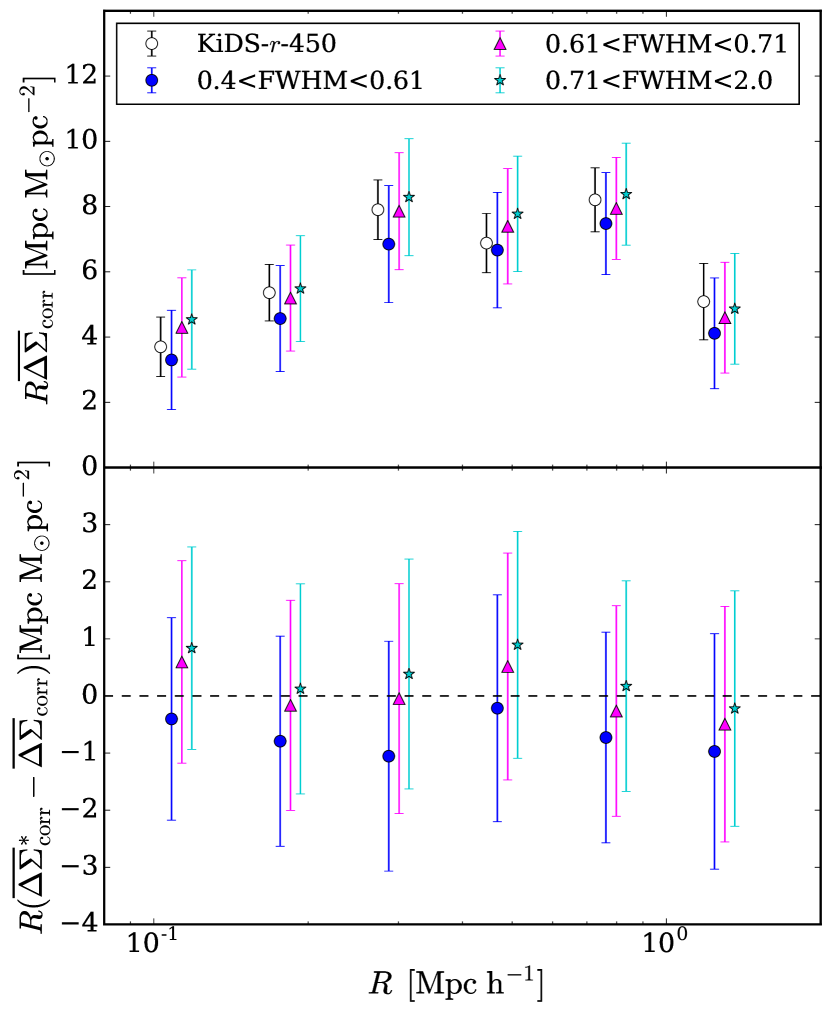
Figure 12: The stacked differential surface mass density measurement $\Delta\Sigma$ for KiDS-$r$-450 with CMASS lenses. The upper panel shows the galaxy-galaxy lensing signal obtained when the the KiDS-$r$-450 sample is split into three samples by seeing. The lower panel shows the difference between these test measurements and the original measurement. All signals are scaled by the comoving separation, $R$, and offset horizontally for clarity.

The middle panel of Figure 11 shows the CMASS excess surface density profiles measured using the full KiDS-$i$-800 dataset, as well as the three seeing subsamples. In each case, a unique boost factor was also calculated and applied, and a corresponding random signal removed. The error is estimated from a Jackknife analysis. The lowest panel highlights the consistency between the measurements made with the different seeing subsamples and the fiducial measurement, noting that the errors will be correlated as a sub-sample is being compared to the entire KiDS-$i$-800 sample. For consistency, Figure 12 shows the results for the equivalent seeing test with the KiDS-$r$-450 galaxies. Again, we find no evidence that variations in the seeing influences the galaxy-galaxy lensing measurement. From these studies we can conclude that our galaxy-galaxy lensing measurements are insensitive to changes in the levels of PSF contamination and seeing.

5 Summary and Outlook

This paper presents $i$-band imaging data from the Kilo-Degree Survey (KiDS-$i$-800). This new lensing dataset spans $815\text{\,}{\mathrm{deg}}^{2}$, with an average effective source density of 3.8 galaxies per square arcmin and a median redshift of $z_{\mathrm{med}}\sim 0.5$. In contrast to the deep $r$-band KiDS observations that make up the homogeneous KiDS multi-band cosmic shear dataset (KiDS-$r$-450), the $i$-band data span a wide range of observing conditions. The less-strict seeing constraints give rise to a very wide range of depth and variation in data quality, weighed against a higher data acquisition rate. We adopt the KiDS data analysis pipeline (Kuijken et al., 2015). This includes the theli software package for data reduction and the self-calibrating version of lensfit for shear measurements, with an adapted methodology for star-galaxy selection in order to reliably select stars in the poorer-seeing $i$-band data.

The combination of KiDS-$i$-800 and KiDS-$r$-450 allows for the first large-scale lensing analysis of two overlapping imaging surveys. We present two ‘null’ tests to uniquely assess the consistency between the weak lensing measurements in both surveys.

In the first test we analyse a matched $ri$ catalogue using a ‘nulled’ two-point shear correlation function. By limiting both surveys to the same matched source sample, we isolate differences between each survey’s shear calibration. By using a two-point correlation function we are sensitive to both additive and multiplicative shear biases. In this study we uncovered significant additive shear bias in the KiDS-$i$-800 survey motivating an extension called the ‘cross-nulled’ two-point shear correlation function. This statistic also nulls additive shear bias if it is uncorrelated between the two surveys. In this ‘cross-nulled’ case we found the two shear calibrations for the matched samples agree at a level of $1\pm 4$ percent. This demonstrates that the differing multiplicative shear calibration corrections for both surveys, produce consistent results between the very different quality KiDS-$i$-800 and KiDS-$r$-450 images.

In the second test we use overlapping spectroscopic surveys to measure a ‘nulled’ galaxy-galaxy lensing signal, for five different lens samples, with the two KiDS lensing datasets. By using the full depth of each lensing survey in this analysis, our results are more applicable in understanding how biases propagate through to final survey results. The consequence, however, is that the ‘nulled’ galaxy-galaxy lensing result can only provide a joint analysis of the shear calibration in combination with the redshift determination. It is also only sensitive to multiplicative shear biases. We therefore recommend the combination of the two null tests that we present in this paper for future shear comparison projects, as they scrutinise the two surveys in different but complementary ways.

One obvious drawback for the single-band KiDS-$i$-800 survey is the inability to determine photometric redshifts for the individual galaxies. Any photometric redshift distribution for the sample therefore cannot be directly inferred. We therefore adopted three different methods to determine an average source redshift distribution for our $i$-band imaging, using overlapping spectroscopy, 30-band photometric redshifts from the COSMOS survey, (COSMOS-30) and a cross-correlation clustering technique. When using the overlapping spectroscopy or the COSMOS-30 data, the KiDS-$i$-800 and KiDS-$r$-450 galaxy-galaxy lensing signals are found to be consistent with a measured excess surface mass density for the two datasets consistent at the level of $7\pm 5$ percent in both cases. When adopting an $i$-band redshift distribution determined through the cross-clustering technique, however, the two datasets differ by $14\pm 4$ percent. These results do not include any uncertainty on the estimates of the redshift distributions. For the cross correlation clustering redshift, in particular, we find this error to be significant at high redshifts. For the other two redshift estimations, while the statistical bootstrap error on the estimation is negligible, we have not quantified any systematic bias of the method resulting from incompleteness in the sample or sampling variance. The spread of the galaxy-galaxy lensing measurements for each lens sample provides some indication of this uncertainty and future scientific analysis of the KiDS-$i$-800 survey will require studies to improve our knowledge of the $i$-band source redshift distribution. We also ‘stress test’ our galaxy-galaxy lensing measurements to highlight that our two datasets are robust against variations in data quality (FWHM) as well as PSF contamination.

The susceptibility of weak lensing measurements to various sources of systematic error provides a strong motivation for the comparison of the lensing signals derived from unique datasets. The $\sim 5$ percent precision afforded by the ‘null’ tests presented in this analysis are unfortunately still far from the percent level precision offered by image simulation studies of shear calibration biases (e.g Fenech Conti et al., 2017). They do however already provide a meaningful and fully independent confirmation of the results from these studies. As overlapping survey area grows these ‘null’ statistics will become an increasingly stringent and required test for weak lensing surveys.

While in this paper we have carried out an internal comparison with our two datasets undergoing a similar data processing procedure, the methodology we have presented can be extended to tests between any set of overlapping surveys. With three on-going lensing surveys that partially overlap, KiDS, the Dark Energy Survey (DES; Jarvis et al., 2016) and Hyper Supreme-Cam (HSC; Aihara et al., 2017), as well as the advent of next-generation surveys like LSST, Euclid and WFIRST, our proposed comparison ‘null’ tests will be an important new addition to ensure robust weak lensing results in the future.

Appendix A Data Reduction and Quality Control

In this paper we use the theli data reduction software to produce lensing quality images in both the $i$- and $r$-band. The theli analysis of the KiDS-$r$-450 data is well documented in Hildebrandt et al. (2016), Kuijken et al. (2015) and de Jong et al. (2013). In this appendix we therefore only highlight the differences in the data reduction between the KiDS-$r$-450 data release and the KiDS-$i$-800 survey. We also discuss the web-based quality control system that we employ to ensure that the final data product is robust.

The two main differences between the KiDS-$r$-450 data reduction and the KiDS-$i$-800 data processing are the need for fringe correction in the $i$-band and the methodology behind the astrometric solution. Fringe-removal was carried out following Section 4.8 of Erben et al. (2005). A fringe model is first built directly from the OmegaCAM imaging, where the fringe geometry pattern has been shown to be very stable over time (de Jong et al., 2015). The amplitude of the fringes to be subtracted from the individual exposures is then assumed to be directly proportional to the sky-background level. As discussed in Erben et al. (2005), this assumption can break down in very bright observing conditions and, as such, the fringe removal of our data is of varying quality. While our procedure works well for the majority of the i-band survey, residual fringing is apparent in some images, as illustrated in Figure 13.

Figure 13: Three examples of chip exposures that would be rejected by our quality control process. The left panel shows sharp changes that are sometimes seen in the gain of the affected Chip 16 (ESO #73). The middle panel reveals electronic defects which can been seen as dark lines across a chip. The right panel shows an example of a low-signal-to-noise satellite track that has not been detected in the co-added image by our automated routine. Once visually identified, the track is manually masked. Note that the grey-scale in this image is set to enhance any low-signal-to-noise features. This setting also highlights the residual low-level fringing that can occasionally be found in the $i$-band imaging, after the removal of a fringe model in the data reduction process.

The differences in astrometric calibration between the $r$ and $i$-band data are as follows: For the $r$-band data we were motivated to adopt a global astrometric solution, as there is almost contiguous coverage in five patches in the $r$-band. This global solution takes into account information from the overlaps between KiDS tiles and data from the overlapping VST ATLAS Survey (Shanks et al., 2015). Given the level of residual fringing in parts of the $i$-band imaging, the KiDS-$i$-800 survey was never intended for the cosmic shear studies that are particularly sensitive to optical camera distortions. The $i$-band astrometry in the KiDS-South patch was therefore only calibrated on a pointing basis including information from the five exposures at slightly different dither positions. This non-global astrometric solution is expected to be less accurate. In the KiDS-North patch, the astrometry for both KiDS-$i$-800 and KiDS-$r$-450 was tied to SDSS-DR12 (Alam et al., 2015) as the reference frame. Both reductions used 2MASS in the South for the absolute astrometric reference frame (Skrutskie et al., 2006).

For KiDS-$i$-800 we developed a new web-based quality control system that allows for distributed work, with two independent checks of each KiDS tile to detect problematic exposures without the requirement to access large FITS files. While the theli data processing is running, the web tool regularly checks for new reduced pointings, adds them automatically to its database, creates a suite of ‘check plots’ and distributes each pointing randomly to two ‘eyeballers’ and informs via e-mail so that an almost instant investigation is possible.

Different categories are available which all have to pass our quality requirements before the pointing is released to the collaboration. These categories are:

• ‘Calibration’, where the bias, dark and flat frames are inspected to identify any corrupted images or unusual features.

• ‘Co-add’, where the stacked image and weight image are verified. Here any catastrophic error in the astrometric solution can be immediately identified with the same objects appearing multiple times.

• ‘Single exposures’, where each individual exposure is checked and flagged if large satellite tracks are identified, or problems are observed on the chip-level.

• ‘Photometry/Astrometry’, where the selection of the stars that are used for the astrometric and photometric solution are checked. The automated star-galaxy separation method that automatically locates the stellar locus in the size-magnitude plane is verified by eye. The astrometric solution is then checked by inspecting the offset between the position of each star in the co-added image and its position in each exposure. Finally the photometry is checked by comparing the measured galaxy number counts, per magnitude bin, to the same galaxy number counts from deep OmegaCAM data of the Chandra Deep Field South (Vaccari et al., 2012).

• ‘Masks’, where the automated stellar halo masks are checked to ensure that all bright stars are masked (see Section 3.4 of Kuijken et al., 2015, for further details). An example mask is shown in Figure 14.

• ‘PSF’, where exposures with a strongly elliptical or rapidly varying point spread function are removed from the stack.

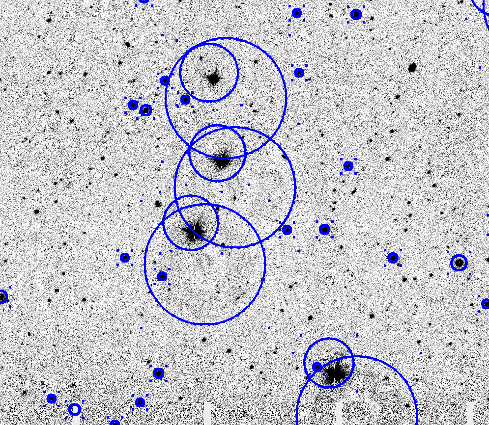
Figure 14: An image section of roughly 20$\mathrm{\SIUnitSymbolArcminute}$ x 20$\mathrm{\SIUnitSymbolArcminute}$ of a KiDS-$i$-800 pointing with our automatically generated stellar masks overlayed. All stars brighter than $i<14.5$ are masked. Stars with $11.5<i<14.5$ are masked with a single, central and circular mask with a radius that scales with object magnitude. Brighter sources are treated with up to three masks covering the stellar core and associated reflection halos. Note that the positions of the reflection halos with respect to the stellar core are strongly variable on the OmegaCAM field-of-view. We found that a two-dimensional second order polynomial describes these variations very accurately.

For each category, any possible issues are listed and can be selected. Depending on the issues found, the pointing is released to the collaboration or is investigated and reprocessed. Examples of cases flagged by this quality control include exposures with electronic defects which appear as lines (see the left panel of Figure 13) and problematic chips with step-changes in the gain (see the middle panel of Figure 13). In addition there are satellite tracks that are not seen in the co-added image and hence not automatically recognised by the theli pipeline, but are clearly visible in the single exposure (right panel of Figure 13). Once identified the problematic chips can be manually excluded and the satellite tracks can be manually masked within the web-interface using JS9. All re-processed data are re-verified until the requirements are met in all quality-control categories, at which point the pointing moves forward to the shape measurement stage of the data analysis pipeline using lensfit (Section 2.3). Note that due to different seeing conditions and PSFs in the five exposures of one pointing, theli does not always use all exposures for co-addition. lensfit has its own quality control criteria to judge if a single exposure is accepted or discarded.

The seeing distribution for the resulting KiDS-$i$-800 data can be compared with the KiDS-$r$-450 data in Figure 7. It is mostly sub-arcsecond and meets the survey requirements ($<$$1.2\text{\,}\mathrm{arcsec}$) with a median of $0.79\text{\,}\mathrm{arcsec}$. For comparison: KiDS-$r$-450 has a median seeing of $0.66\text{\,}\mathrm{arcsec}$. However, the $i$-band distribution is very broad and this is reflected in the broad range of limiting magnitudes with $i_{\rm lim}=22.7\pm 0.3$, where the $5\sigma$ limiting magnitude is defined within a $2\text{\,}\mathrm{arcsec}$ radius.

Appendix B Selection criteria

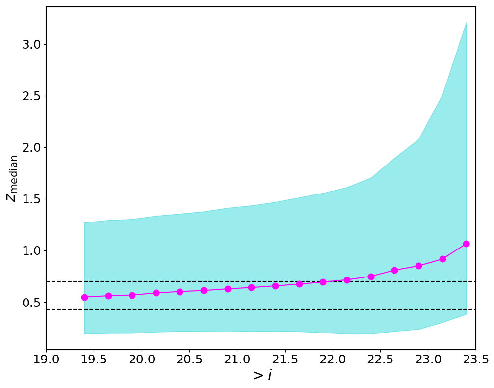
Figure 15: The median redshift for the KiDS-$i$-800 redshift distribution, estimated using the SPEC method as a function of the lower $i-$band magnitude limit. The shaded range represents the lower and upper quartile spread of the distribution.

In section 3 we introduce a selection on $i$-band magnitude in order to increase the average redshift of the sample. Figure 15 shows the median redshift of the distribution, estimated using the SPEC method (section 3.3), as a function of the lower limit $i-$band magnitude. The turquoise shaded region corresponds to the the upper and lower quartile of the distribution. Dashed lines indicate the maximum redshift for the LZ and HZ lens samples, $z_{l}<0.43$ and $z_{l}<0.7$. For KiDS-$r$-450, sources are selected to be behind each lens slice according to their photometric redshift with $z_{\rm B}>z_{l}+0.1$. As this was not possible for KiDS-$i$-800, Figure 15 was used to optimise the $i$-band magnitude selection. In order to achieve a sample with a median redshift that was deeper than the maximum lens redshift, galaxies were selected to have $i>20.8$ for the analysis of the higher redshift HZ lenses. The lensfit selection criteria of $i>19.4$, see Section 2.3, is shown to be suitable for the analysis of the low redshift LZ lenses.

Appendix C Comparison of selected KiDS stars with Gaia DR1

The Gaia mission is on course to create a fully three-dimensional map of the objects in our Milky-Way galaxy, measuring accurate $G$-band photometry, astrometry and proper motion for almost a billion point-like sources. In this appendix we use data from the first year of observations (DR1; Gaia Collaboration et al., 2016) to explore the levels of galaxy contamination in the star catalogue that is used to create PSF models in Section 2.2. We match the Gaia-DR1 source list with KiDS object catalogues using a $0.2\text{\,}\mathrm{a}\mathrm{r}\mathrm{c}\mathrm{s}\mathrm{e}\mathrm{c}$ search radius. We do not apply any filtering to the Gaia catalogue as problematic cases and spurious sources have already been removed from the sample (Gaia Collaboration et al., 2016). This first-look at the Gaia data shows that, once fully complete, Gaia will provide a very promising resource for future accurate PSF modelling.

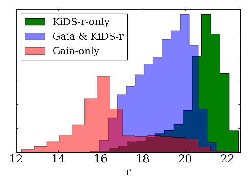
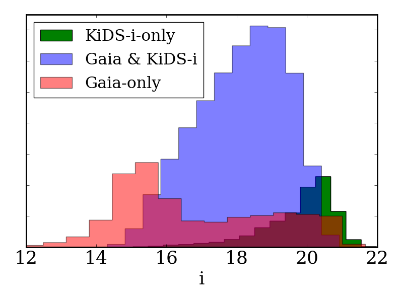
Figure 16: The magnitude distribution of three different stellar samples as a function of their KiDS-measured magnitude, $r$-band (left) and $i$-band (right). In red, Gaia objects that are not used to determine the KiDS PSF model. In blue, Gaia objects that are used in the KiDS PSF model. In green, objects that are used to determine the KiDS PSF model, but are not present in the Gaia catalogues.

Figure 16 compares the magnitude distribution of three different samples as a function of their KiDS-measured magnitude, $r$-band (left) and $i$-band (right). The brightest sample contains Gaia objects that are not used to determine the KiDS PSF model (shown in red). The majority of these objects are saturated in the KiDS-imaging. The faintest sample contains objects that are used to determine the KiDS PSF model, but are not present in the Gaia catalogues (shown in green). The majority of these objects are too faint to be detected given the Gaia flux limit $G<20$. The centre sample (shown in blue) are Gaia objects that are used in the KiDS PSF model. Where the objects have been used in the KiDS PSF model, we present a weighted distribution determined from the weight given to each object in the PSF model. Comparing the results for KiDS-$r$-450 (left) and KiDS-$i$-800 (right) we find that the star catalogue is significantly deeper in the $r$-band, as expected given the exposure time. Both star catalogues, however, show a tail of brighter objects that are not detected by Gaia but are within the nominal Gaia magnitude limits. Both also show a tail of fainter Gaia objects that are not used in the PSF modelling but are within the KiDS saturation limits.

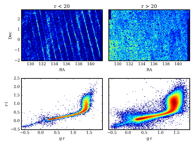
Figure 17: Upper panels: The on-sky distribution of the KiDS-$r$-only stars for the ‘G9’ field, split by magnitude, with $r<20.5$ (left) and $r>20.5$ (right), revealing the Gaia-DR1 scanning pattern. Lower panels: $(r-i)-(g-r)$ colour-colour diagrams that follow the expected stellar locus. In all panels the colour scale increases from dark blue (few objects) through to red. The upper panels use a linear scale, the lower panels use a log-scale.

Figure 17 shows the on-sky distribution of the KiDS-$r$-only stars for the ‘G9’ field, split by magnitude with a bright sample ($r<20.5$, shown left) and a faint sample ($r>20.5$, shown right). In this first Gaia data release the scanning pattern is such that some stripes of sky have been visited more often than others. This is seen in the left panel of Figure 17 where the variable on-sky incompleteness is reflected as stripes in the faint star number density. On the completion of Gaia, the survey depth will be homogenous. For the faint sample, in contrast, the on-sky distribution is relatively smooth. The same patterns are found when inspecting the on-sky distribution of the KiDS-$i$-only stars. The lower panels of Figure 17 show that the faint and bright samples from the selected KiDS-$r$-only stars closely follow a stellar-locus in this colour-colour diagram. We therefore conclude that our star selection is robust and not subject to significant galaxy contamination.

We investigated the Gaia sources that were not used as input to constrain our PSF model. We carried out a visual inspection of Gaia objects with a KiDS $r$-band magnitude that was significantly brighter than the Gaia $G$-band magnitude, with $r-G>0.5$. This revealed that $\sim 7\%$ of the Gaia objects not used in the PSF modelling were actually bright galaxies where Gaia had only resolved the core. This galaxy contamination contributes at the level of $\sim 3\%$ to the full Gaia-DR1 catalogue. Other Gaia sources were flagged as unusable in KiDS through image defects, but this effect does not account for the full missing Gaia sample in our KiDS star catalogue. This suggests that selection bias could have been introduced during our star selection. We note that the fraction of unsaturated Gaia sources not used in the PSF modelling is higher for our $i$-band (14%) compared to our $r$-band (10%).

In principle, Gaia could also be used to determine the level of stellar contamination in our galaxy sample. For our KiDS sample we impose a bright magnitude cut at $r>20.0$ and $i>19.4$ owing to limitations in the accuracy of shear calibration correction in this regime (see Fenech Conti et al., 2017). As Figure 16 therefore shows, the overlap between this galaxy sample and the Gaia depth is minimal and so what we can learn about stellar contamination of our galaxy catalogue, from Gaia is limited.

Appendix D Corrections to the galaxy-galaxy lensing signal

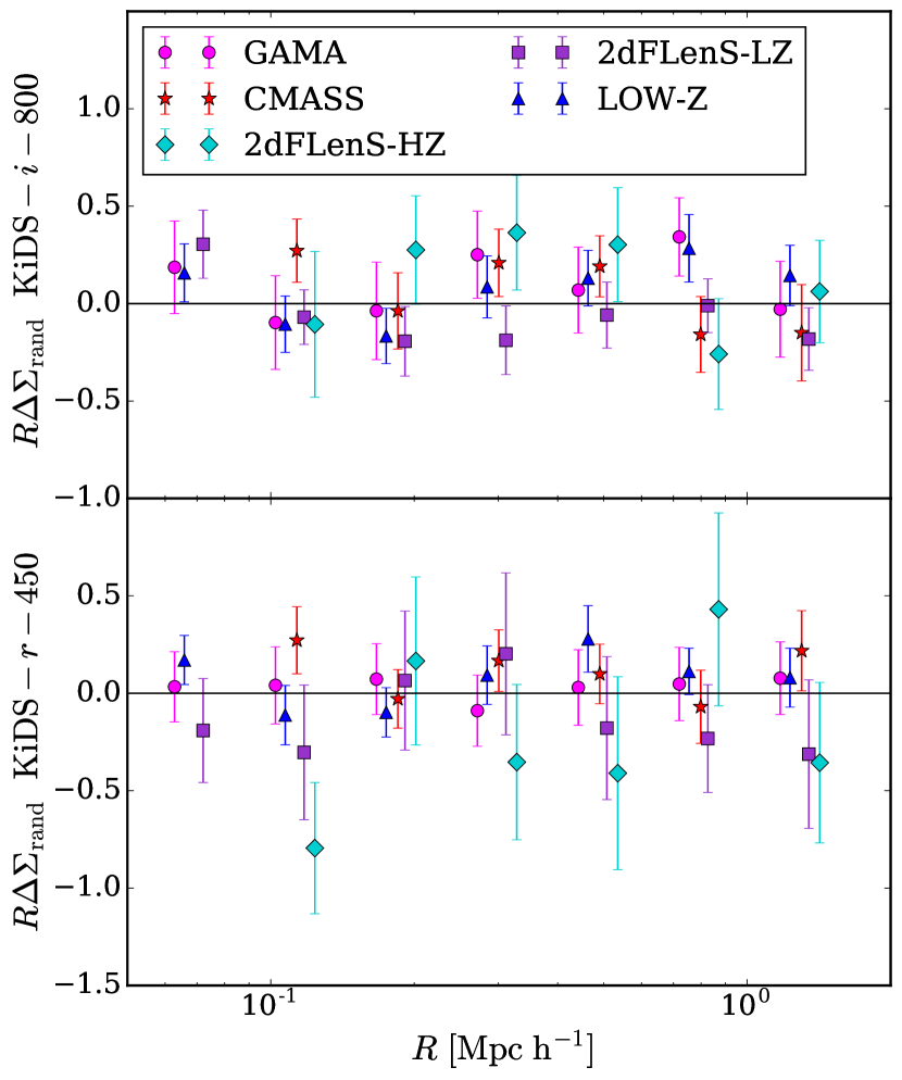
Figure 18: The random galaxy-galaxy lensing signals $\Delta\Sigma(R)_{\rm rand}$ for KiDS-$i$-800 (upper) and KiDS-$r$-450 (lower) for each of the lens samples. The errors show the standard error on the mean of the forty random signals computed.

In this appendix we present details of the ‘random signal’ and ‘boost correction’ that are used to correct for errors arising from additive bias, sampling variance and lens-source clustering in our galaxy-galaxy lensing measurements (see equation 29).

Random lens catalogues are created for each spectroscopic sample by preserving the redshift distribution of the lenses but replacing their positions with random points generated with the angular mask of the survey area. Galaxy-galaxy lensing measurements are then determined for each source sample using 40 independent random catalogues for each lens sample. These ‘random signals’, $\Delta\Sigma_{\rm rand}$, are presented for each spectroscopic sample in Figure 18 using the KiDS-$i$-800 source galaxies in the upper panel and KiDS-$r$-450 in the lower. The error bars represent the error on the mean of the signal from 40 realisations of the signals and show the ‘random’ signal to be consistent with zero. We still correct our galaxy-galaxy lensing measurements with this signal, however, as Singh et al. (2016) has shown, this correction reduces sampling variance errors. The error on the mean random signal is propagated through to the final error on the corrected $\Delta\Sigma(R)^{\rm corr}$ measurement.

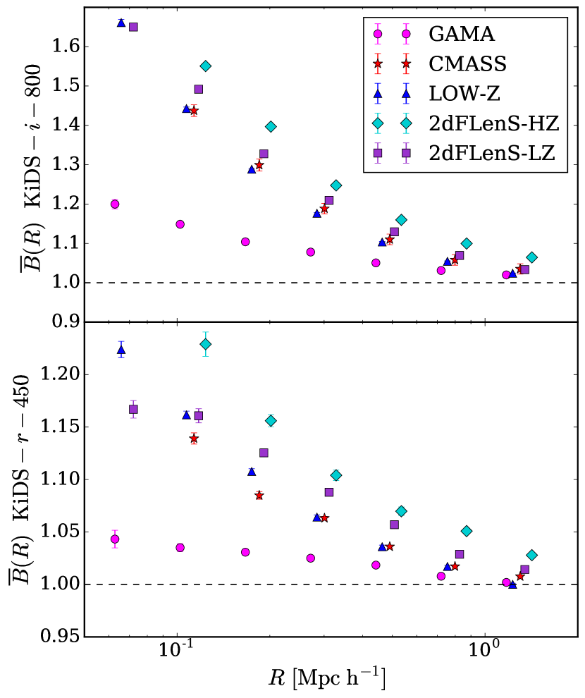
Figure 19: The boost factors for KiDS-$i$-800 (upper) and KiDS-$r$-450 (lower) that account for a dilution of the galaxy-galaxy lensing signal due to sources being associated with the lenses. The errors represent the standard error on the mean of the ten realisations computed and are consistent with the size of the data-points.

The boost factors $\overline{B}({R})$, are computed as a function of projected separation as an average over each of the lens slices, for each of the measurements according to equation 28 and shown in Figure 19. Contamination by sources that are associated with the lens biases the lensing signal low by a factor that is equal to the overdensity of sources around the lenses; hence we can correct the lensing signal by multiplying it by the boost factor. We make 10 independent measurements of the boost factor for each lens sample with both KiDS-$i$-800 and the KiDS-$r$-450 using unique realisations of the random lens catalogue. The mean of these are plotted in Figure 19 with the error on the mean of the ten realisations represented by the errorbars. On scales $R<2h^{-1}{\rm Mpc}$ we find boost signals $\overline{B}(R)>1$ showing that the source sample on these scales is contaminated by galaxies that are associated with the lenses. Note that as the errors on the boost factors are small, we do not propagate these errors through to the final error on the corrected $\Delta\Sigma(R)^{\rm corr}$ measurement.

As expected, the corrections for the KiDS-$i$-800 galaxies, shown in the upper panel, are larger than those of KiDS-$r$-450, in the lower panel. By limiting KiDS-$r$-450 lensing galaxies to only those with a photometric redshift behind each lens slice by $z_{B}>z_{l}+0.1$ we decrease the overall number of sources associated with the lens and therefore lower the boost correction, compared to that of KiDS-$i$-800, where this photometric redshift selection is not possible. However, as redshift distributions for the source redshifts are still broad, this ‘boost factor’ is still non-negligible for KiDS-$r$-450. For both lensing samples, the boost factors are highest for the high redshift and then low redshift 2dFLenS galaxies. As was the case for the galaxy-galaxy lensing measurements shown in Figure 9, these lens samples contain the largest fraction of LRG galaxies, which have a higher galaxy bias and therefore the greatest possible association compared to the BOSS samples. For both 2dFLenS and BOSS, the high redshift lens samples have a greater overlap with the redshift distributions of the source galaxies and so a higher fraction of the source sample will be associated with the lenses. For the KiDS-$i$-800 sample, the boost factor is as high as 50% at $0.1h^{-1}$ Mpc and for the KiDS-$r$-450 galaxies the boost correction is at the level of 20%. In both cases, the corrections taper to one beyond $2.0h^{-1}$ Mpc.

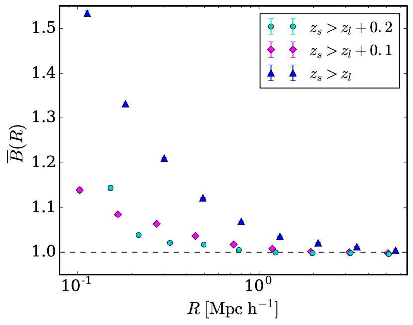
Figure 20: The measured boost factors for KiDS-$r$-450 with different source galaxy selections. More stringent limitations of sources to those behind the lenses reduce the number of sources associated with the lenses, thereby reducing the boost factor. The errors represent the standard error on the mean of the ten realisations computed and are consistent with the size of the data-points.

For the KiDS-$r$-450 measurements, we investigated the optimal source redshift cut to minimise the contamination of galaxies that are physically associated with the lenses. While this contamination is entirely accounted for by an accurate boost factor, the errors are also inflated by this factor. On the other hand, the contamination of source galaxies associated with the lens can be further suppressed by applying more aggressive cuts to the source sample, but this also removes real source galaxies and undesirably decreases the lensing signal-to-noise ratio. Figure 20 compares the boost factor measured around CMASS galaxies for our fiducial galaxy selection, with a less and more stringent $z_{\rm B}$ selection. Limiting source galaxies to $z_{B}>z_{l}$ more than doubles the level of contamination, resembling the boost factors computed for the KiDS-$i$-800 galaxies.

Appendix E Analytical Covariance for the ‘nulled’ two-point shear correlation function

We model the observed ellipticity in terms of a number of components (equation 5), which for $\gamma<<1$, in the absence of systematic errors, can be written as

$$\epsilon^{\mathrm{obs}}=\gamma+\epsilon^{\mathrm{int}}+\epsilon^{\mathrm{n}}\,,$$ (33)

where $\epsilon^{\mathrm{int}}$ is the galaxy’s intrinsic ellipticity, $\epsilon^{\mathrm{n}}$ is the random noise on the measured galaxy ellipticity which will increase as the signal-to-noise of the galaxy decreases, and $\gamma$ is the true lensing-induced shear that we wish to detect. With this model, the shear correlation function $\xi_{\pm}$ (equation 9) can be expanded into a series of terms

$$\xi_{\rm tot}=\xi_{\gamma\gamma}+\xi_{\rm int\,int}+\xi_{\rm nn}+2\xi_{\rm n\,int}+2\xi_{\rm n\gamma}+2\xi_{\rm\gamma\,int}\,,$$ (34)

where the subscripts indicate the correlation between the different components that contribute to the observed ellipticity measurements. The two ‘nulled’ shear correlation functions in equations 11 and 12 can be written in this form with

$$\xi_{\rm tot}^{\rm null} = \xi_{\rm tot}^{ii}-\xi_{\rm tot}^{rr}$$

$$= \xi_{\rm nn}^{ii}-\xi_{\rm nn}^{rr}+2(\xi^{i}_{\rm n\,int}-\xi^{r}_{\rm n\,int})\,,$$

$$\xi_{\rm tot}^{\rm x-null} = \xi_{\rm tot}^{ir}-\xi_{\rm tot}^{rr}$$

$$= \xi_{\rm nn}^{ir}-\xi_{\rm nn}^{rr}+\xi^{i}_{\rm n\,int}-\xi^{r}_{\rm n\,int}\,,$$

where the superscripts $r$ and $i$ indicate the combination of filters that are being analysed. In this derivation we have assumed that terms which include the correlation between measurement noise and shear are sufficiently small that they can be ignored. We also assume that the intrinsic ellipticity $\epsilon^{\mathrm{int}}$ does not change significantly between the two filters (as shown by Jarvis & Jain, 2008). With these assumptions we see that all terms that include the shear cancel, leaving only intrinsic and shape measurement noise terms.

The auto-noise covariance matrix for the shear correlation function is diagonal with

$$C_{\rm nn}(\theta_{j},\theta_{j})=\frac{4\sigma_{\rm n}^{4}}{N_{p}(\theta_{j})}\,,$$ (35)

where $\sigma_{\rm n}$ is the per component ellipticity dispersion of $\epsilon^{\mathrm{n}}$, and $N_{p}(\theta_{j})$ is the number of pairs in angular bin, $j$, (see equation 15), derived analogously to Schneider et al. (2002). The cross-covariance for the noise between the two filters is also diagonal with

$$C_{\rm nn}^{ir}(\theta_{j},\theta_{j})=\frac{2\sigma_{\rm{n},i}^{2}\sigma_{\rm{n},r}^{2}}{N_{p}(\theta_{j})}\,,$$ (36)

where we assume that the shape measurement noise is independent of the intrinsic shape of the galaxy and hence is uncorrelated between bands. Under this assumption, the cross covariance between the shape noise and intrinsic ellipticity noise is also diagonal with

$$C_{\rm n\,int}(\theta_{j},\theta_{j})=\frac{2\sigma_{\rm n}^{2}\sigma_{\rm int}^{2}}{N_{p}(\theta_{j})}\,.$$ (37)

With an educated guess for the value of the intrinsic ellipticity dispersion $\sigma_{\rm int}$, we can calculate $\sigma_{\rm n}$ from the observed ellipticity dispersion $\sigma_{\epsilon}$ (equation 8) as $\sigma_{\epsilon}^{2}=\sigma_{\rm n}^{2}+\sigma_{\rm int}^{2}$. We use the notation of $\sigma_{i}$ for the measured ellipticity dispersions in the $i$-band images and $\sigma_{r}$ for that of the $r$-band. We can then derive an analytical covariance for the two ‘nulled’ shear correlation functions with

$$C^{\rm null}_{\xi}(\theta_{j},\theta_{j}) = C_{\rm nn}^{rr}+C_{\rm nn}^{ii}+4(C_{\rm n\,int}^{r}+C_{\rm n\,int}^{i})$$

$$= \frac{4}{N_{p}(\theta_{j})}(\sigma^{4}_{i}+\sigma^{4}_{r}-2\sigma^{4}_{\rm int})\,,$$

$$C^{\rm x-null}_{\xi}(\theta_{j},\theta_{j}) = C_{\rm nn}^{rr}+C_{\rm nn}^{ir}+C_{\rm n\,int}^{r}+C_{\rm n\,int}^{i}$$

$$= \frac{2}{N_{p}(\theta_{j})}[2\sigma^{4}_{r}+\sigma^{4}_{\rm int}+\sigma^{2}_{r}(\sigma^{2}_{i}-4\sigma^{2}_{\rm int})]\,,$$

where again the superscripts $r$ and $i$ indicate the combination of filters that are being analysed.

References

- Aihara et al. (2017) Aihara H., et al., 2017, preprint, (arXiv:1704.05858)
- Alam et al. (2015) Alam S., et al., 2015, ApJS, 219, 12
- Alam et al. (2017) Alam S., Miyatake H., More S., Ho S., Mandelbaum R., 2017, MNRAS, 465, 4853
- Amon et al. (2017) Amon A., et al., 2017, preprint, (arXiv:1711.10999)
- Bartelmann & Schneider (2001) Bartelmann M., Schneider P., 2001, Phys. Rep., 340, 291
- Becker et al. (2016) Becker M. R., et al., 2016, Phys. Rev. D, 94, 022002
- Benítez (2000) Benítez N., 2000, ApJ, 536, 571
- Bertin & Arnouts (1996) Bertin E., Arnouts S., 1996, A&AS, 117, 393
- Blake et al. (2016a) Blake C., et al., 2016a, MNRAS, 456, 2806
- Blake et al. (2016b) Blake C., et al., 2016b, MNRAS, 462, 4240
- Chang et al. (2013) Chang C., et al., 2013, MNRAS, 434, 2121
- Choi et al. (2016) Choi A., et al., 2016, MNRAS, 463, 3737
- Dawson et al. (2013) Dawson K. S., et al., 2013, AJ, 145, 10
- Driver et al. (2011) Driver S. P., et al., 2011, MNRAS, 413, 971
- Dvornik et al. (2017) Dvornik A., et al., 2017, MNRAS, 468, 3251
- Dvornik et al. (2018) Dvornik A., et al., 2018, preprint, (arXiv:1802.00734)
- Eisenstein et al. (2011) Eisenstein D. J., et al., 2011, AJ, 142, 72
- Erben et al. (2005) Erben T., et al., 2005, Astronomische Nachrichten, 326, 432
- Erben et al. (2009) Erben T., et al., 2009, A&A, 493, 1197
- Erben et al. (2013) Erben T., et al., 2013, MNRAS, 433, 2545
- Fenech Conti et al. (2017) Fenech Conti I., Herbonnet R., Hoekstra H., Merten J., Miller L., Viola M., 2017, MNRAS, 467, 1627
- Gaia Collaboration et al. (2016) Gaia Collaboration Brown A. G. A., Vallenari A., Prusti T., de Bruijne J., Mignard F., Drimmel R., co-authors ., 2016, preprint, (arXiv:1609.04172)
- Griffith et al. (2012) Griffith R. L., et al., 2012, ApJS, 200, 9
- Hand et al. (2015) Hand N., et al., 2015, Phys. Rev. D, 91, 062001
- Heymans et al. (2005) Heymans C., et al., 2005, MNRAS, 361, 160
- Heymans et al. (2006) Heymans C., et al., 2006, MNRAS, 368, 1323
- Heymans et al. (2012a) Heymans C., Rowe B., Hoekstra H., Miller L., Erben T., Kitching T., van Waerbeke L., 2012a, MNRAS, 421, 381
- Heymans et al. (2012b) Heymans C., et al., 2012b, MNRAS, 427, 146
- Hildebrandt et al. (2016) Hildebrandt H., et al., 2016, MNRAS,
- Hildebrandt et al. (2017) Hildebrandt H., et al., 2017, MNRAS, 465, 1454
- Hirata et al. (2004) Hirata C. M., et al., 2004, MNRAS, 353, 529
- Hoekstra (2004) Hoekstra H., 2004, MNRAS, 347, 1337
- Hoekstra & Jain (2008) Hoekstra H., Jain B., 2008, Annual Review of Nuclear and Particle Science, 58, 99
- Hoekstra et al. (2004) Hoekstra H., Yee H. K. C., Gladders M. D., 2004, ApJ, 606, 67
- Hoekstra et al. (2005) Hoekstra H., Hsieh B. C., Yee H. K. C., Lin H., Gladders M. D., 2005, ApJ, 635, 73
- Ilbert et al. (2009) Ilbert O., et al., 2009, ApJ, 690, 1236
- Jarvis & Jain (2008) Jarvis M., Jain B., 2008, J. Cosmology Astropart. Phys., 1, 003
- Jarvis et al. (2016) Jarvis M., et al., 2016, MNRAS, 460, 2245
- Jee et al. (2013) Jee M. J., Tyson J. A., Schneider M. D., Wittman D., Schmidt S., Hilbert S., 2013, ApJ, 765, 74
- Johnson et al. (2017) Johnson A., et al., 2017, MNRAS, 465, 4118
- Kilbinger (2015) Kilbinger M., 2015, Reports on Progress in Physics, 78, 086901
- Kilbinger et al. (2014) Kilbinger M., Bonnett C., Coupon J., 2014, athena: Tree code for second-order correlation functions, Astrophysics Source Code Library (ascl:1402.026)
- Kleinheinrich et al. (2004) Kleinheinrich M., et al., 2004, ArXiv Astrophysics e-prints,
- Komatsu et al. (2011) Komatsu E., et al., 2011, ApJS, 192, 18
- Kuijken et al. (2015) Kuijken K., et al., 2015, MNRAS, 454, 3500
- Kwan et al. (2017) Kwan J., et al., 2017, MNRAS, 464, 4045
- Laigle et al. (2016) Laigle C., et al., 2016, ApJS, 224, 24
- Leauthaud et al. (2017) Leauthaud A., et al., 2017, MNRAS, 467, 3024
- Lilly et al. (2009) Lilly S. J., et al., 2009, ApJS, 184, 218
- Lima et al. (2008) Lima M., Cunha C. E., Oyaizu H., Frieman J., Lin H., Sheldon E. S., 2008, MNRAS, 390, 118
- Liske et al. (2015) Liske J., et al., 2015, MNRAS, 452, 2087
- Mandelbaum et al. (2005) Mandelbaum R., et al., 2005, MNRAS, 361, 1287
- Mandelbaum et al. (2006) Mandelbaum R., Seljak U., Kauffmann G., Hirata C. M., Brinkmann J., 2006, MNRAS, 368, 715
- Mandelbaum et al. (2017) Mandelbaum R., et al., 2017, preprint, (arXiv:1705.06745)
- Melchior & Viola (2012) Melchior P., Viola M., 2012, MNRAS, 424, 2757
- Ménard et al. (2013) Ménard B., Scranton R., Schmidt S., Morrison C., Jeong D., Budavari T., Rahman M., 2013, preprint, (arXiv:1303.4722)
- Miller et al. (2013) Miller L., et al., 2013, MNRAS, 429, 2858
- Miyatake et al. (2015a) Miyatake H., et al., 2015a, ApJ, 806, 1
- Miyatake et al. (2015b) Miyatake H., et al., 2015b, ApJ, 806, 1
- Morrison et al. (2017) Morrison C. B., Hildebrandt H., Schmidt S. J., Baldry I. K., Bilicki M., Choi A., Erben T., Schneider P., 2017, MNRAS, 467, 3576
- Nakajima et al. (2012) Nakajima R., Mandelbaum R., Seljak U., Cohn J. D., Reyes R., Cool R., 2012, MNRAS, 420, 3240
- Newman et al. (2013) Newman J. A., et al., 2013, ApJS, 208, 5
- Planck Collaboration et al. (2016) Planck Collaboration et al., 2016, A&A, 594, A13
- Rahman et al. (2016) Rahman M., Mendez A. J., Ménard B., Scranton R., Schmidt S. J., Morrison C. B., Budavári T., 2016, MNRAS, 460, 163
- Ross et al. (2012) Ross A. J., et al., 2012, MNRAS, 424, 564
- Schirmer (2013) Schirmer M., 2013, ApJS, 209, 21
- Schmidt et al. (2013) Schmidt S. J., Ménard B., Scranton R., Morrison C., McBride C. K., 2013, MNRAS, 431, 3307
- Schneider (2016) Schneider P., 2016, A&A, 592, L6
- Schneider et al. (2002) Schneider P., van Waerbeke L., Kilbinger M., Mellier Y., 2002, A&A, 396, 1
- Schrabback et al. (2016) Schrabback T., et al., 2016, preprint, (arXiv:1611.03866)
- Scoville et al. (2007) Scoville N., et al., 2007, ApJS, 172, 1
- Seitz & Schneider (1997) Seitz C., Schneider P., 1997, A&A, 318, 687
- Shanks et al. (2015) Shanks T., et al., 2015, MNRAS, 451, 4238
- Singh et al. (2016) Singh S., Mandelbaum R., Seljak U., Slosar A., Vazquez Gonzalez J., 2016, preprint, (arXiv:1611.00752)
- Skrutskie et al. (2006) Skrutskie M. F., et al., 2006, AJ, 131, 1163
- Troxel et al. (2017) Troxel M. A., et al., 2017, preprint, (arXiv:1708.01538)
- Vaccari et al. (2010) Vaccari M., et al., 2010, A&A, 518, L20
- Vaccari et al. (2012) Vaccari M., et al., 2012, in Science from the Next Generation Imaging and Spectroscopic Surveys. p. 49
- Viola et al. (2014) Viola M., Kitching T. D., Joachimi B., 2014, MNRAS, 439, 1909
- Viola et al. (2015) Viola M., et al., 2015, MNRAS, 452, 3529
- Voigt & Bridle (2010) Voigt L. M., Bridle S. L., 2010, MNRAS, 404, 458
- Voigt et al. (2012) Voigt L. M., Bridle S. L., Amara A., Cropper M., Kitching T. D., Massey R., Rhodes J., Schrabback T., 2012, MNRAS, 421, 1385
- Wittman et al. (2002) Wittman D. M., et al., 2002, in Tyson J. A., Wolff S., eds, Proc. SPIEVol. 4836, Survey and Other Telescope Technologies and Discoveries. pp 73–82 (arXiv:astro-ph/0210118), doi:10.1117/12.457348
- Wolf et al. (2017) Wolf C., et al., 2017, MNRAS, 466, 1582
- de Jong et al. (2013) de Jong J. T. A., Verdoes Kleijn G. A., Kuijken K. H., Valentijn E. A., 2013, Experimental Astronomy, 35, 25
- de Jong et al. (2015) de Jong J. T. A., et al., 2015, A&A, 582, A62
- de Jong et al. (2017) de Jong J. T. A., et al., 2017, preprint, (arXiv:1703.02991)
- van Uitert et al. (2011) van Uitert E., Hoekstra H., Velander M., Gilbank D. G., Gladders M. D., Yee H. K. C., 2011, A&A, 534, A14
- van Uitert et al. (2016) van Uitert E., et al., 2016, MNRAS, 459, 3251