Tidal stripping and the structure of dwarf galaxies in the Local Group

Abstract

The shallow faint-end slope of the galaxy mass function is usually reproduced in $\Lambda$CDM galaxy formation models by assuming that the fraction of baryons that turns into stars drops steeply with decreasing halo mass and essentially vanishes in haloes with maximum circular velocities $V_{\rm max}<20$–$30\,{\rm km}\,\,{\rm s}^{-1}$. Dark matter-dominated dwarfs should therefore have characteristic velocities of about that value, unless they are small enough to probe only the rising part of the halo circular velocity curve (i.e., half-mass radii, $r_{1/2}\ll 1$ kpc). Many dwarfs have properties in disagreement with this prediction: they are large enough to probe their halo $V_{\rm max}$ but their characteristic velocities are well below $20\,{\rm km}\,\,{\rm s}^{-1}$. These ‘cold faint giants’ (an extreme example is the recently discovered Crater 2 Milky Way satellite) can only be reconciled with our $\Lambda$CDM models if they are the remnants of once massive objects heavily affected by tidal stripping. We examine this possibility using the APOSTLE cosmological hydrodynamical simulations of the Local Group. Assuming that low velocity dispersion satellites have been affected by stripping, we infer their progenitor masses, radii, and velocity dispersions, and find them in remarkable agreement with those of isolated dwarfs. Tidal stripping also explains the large scatter in the mass discrepancy-acceleration relation in the dwarf galaxy regime: tides remove preferentially dark matter from satellite galaxies, lowering their accelerations below the $a_{\rm min}\sim 10^{-11}{\,{\rm m}\,{\rm s}^{-2}}$ minimum expected for isolated dwarfs. In many cases, the resulting velocity dispersions are inconsistent with the predictions from Modified Newtonian Dynamics, a result that poses a possibly insurmountable challenge to that scenario.

1 Introduction

The standard model of cosmology, Lambda Cold Dark Matter ($\Lambda$CDM), makes clear predictions for the dark halo mass function once the cosmological parameters are specified (Jenkins et al., 2001; Tinker et al., 2008; Angulo et al., 2012). At the low mass end, this is much steeper than the faint end of the galaxy stellar mass function, an observation that precludes a simple, linear relation between galaxy and halo masses at the faint end. The difference can be resolved if galaxies fail to form in haloes below some ‘threshold’ mass; this confines galaxies to relatively massive haloes, preventing the formation of large numbers of faint dwarfs and reconciling the faint-end slope of the galaxy luminosity function with the predictions of $\Lambda$CDM (see, e.g., White & Frenk, 1991; Benson et al., 2003, and references therein).

This is not simply an ad-hoc solution. QSO studies have long indicated that the Universe reionized soon after the first stars and galaxies formed ($z_{\rm reion}\lesssim 8$; see, e.g., Fan et al., 2006), an event that heated the intergalactic medium to the ionization energy of hydrogen, evaporating it away from low-mass haloes and proto-haloes, especially from those that had not yet been able to collapse. In slightly more massive haloes, where gas is able to collapse, vigorous winds powered by the energy of the first supernovae expel the remaining gas. These processes thus provide a natural explanation for the steeply declining galaxy formation efficiency with decreasing halo mass required to match the faint end of the galaxy stellar mass function. Cosmological galaxy formation simulations, such as those from the APOSTLE/EAGLE (Schaye et al., 2015; Sawala et al., 2016b) or Illustris projects (Vogelsberger et al., 2014) rely heavily on this mechanism to explain not only the faint-end of the luminosity function, but also the abundance of Galactic satellites, their stellar mass distribution, and their dark matter content (see; e.g., Sawala et al., 2016a).

Simulations like APOSTLE predict a tight correlation between galaxy mass and halo mass; given the stellar mass of a galaxy, $M_{\rm str}$, its halo mass is constrained to better than $\sim~{}15$ per cent in the dwarf galaxy regime, defined hereafter as $M_{\rm str}<10^{9}\,M_{\odot}$. Because of the steep mass dependence of the galaxy formation efficiency in this mass range the converse is not true: at a given halo mass galaxies scatter over decades in stellar mass, in agreement with the latest semi-analytic models of galaxy formation (Moster et al., 2017). This is especially true of ‘faint dwarfs’, defined as those fainter than $M_{\rm str}\sim 10^{7}\,M_{\odot}$ (about the mass of the Fornax dwarf spheroidal), which are all expected to form in haloes of similar mass, or, more specifically, haloes with maximum circular velocity in the range $20\lesssim V_{\rm max}/{\rm km\,s}^{-1}\lesssim 30$ (see; e.g., Okamoto & Frenk, 2009; Sawala et al., 2016b; Oman et al., 2016).

This observation has a couple of important corollaries. One is that, since the dark mass profile of CDM haloes is well constrained (Navarro et al., 1996b, 1997, hereafter NFW), the dark matter content of faint dwarfs should depend tightly on their size: physically larger galaxies are expected to enclose more dark matter and have, consequently, higher velocity dispersions. A second corollary is that galaxies large enough to sample radii close to $r_{\rm max}$, where the halo circular velocity reaches its maximum value, $V_{\rm max}$, should all have similar characteristic circular velocities of order $20$–$30\,{\rm km}\,\,{\rm s}^{-1}$ , reflecting the narrow range of their parent halo masses. For this velocity range, $r_{\rm max}$ is expected to be of order $\sim 3$–$6$ kpc, and faint dwarfs as large as $\sim 1$ kpc should have circular velocities well above $\sim~{}15\,{\rm km}\,\,{\rm s}^{-1}$.

At first glance, these corollaries seem inconsistent with the observational evidence. Indeed, there is little correlation between velocity dispersion and size in existing faint dwarf samples, and there are a number of dwarfs that, although large enough to sample radii close to $r_{\rm max}$, still have velocity dispersions well below $\sim 20\,{\rm km}\,\,{\rm s}^{-1}$. A prime example is the recently discovered Crater 2 dwarf spheroidal (Torrealba et al., 2016), termed a ‘cold faint giant’ for its large size (projected half-mass radius $r_{1/2}\sim 1$ kpc), low stellar mass ($M_{\rm str}\sim 10^{5}\,M_{\odot}$) and small velocity dispersion ($\sigma_{\rm los}\sim 3\,{\rm km}\,\,{\rm s}^{-1}$, Caldwell et al., 2017). The basic disagreement between the relatively large velocities expected for dwarfs and the low values actually measured is at the root of a number of ‘challenges’ to $\Lambda$CDM on small scales identified in recent years (see, e.g., the recent reviews by Del Popolo & Le Delliou, 2017; Bullock & Boylan-Kolchin, 2017).

Before rushing to conclude that these problems signal the need for a radical change in the cold dark matter paradigm, it is important to recall that the corollaries listed above rest on two important assumptions: one is that (i) the assembly of a dwarf does not change appreciably the dark matter density profile, and another is that (ii) dwarfs have evolved in isolation and have not been subject to the effects of external tides, which may in principle substantially alter their dark matter and stellar content.

The first issue has been heavily debated in the literature, where, depending on the algorithmic choice made for star formation and feedback, simulations show that the baryonic assembly of the galaxy can in principle reduce the central density of dark matter haloes and create ‘cores’ (Navarro et al., 1996a; Read & Gilmore, 2005; Mashchenko et al., 2006; Governato et al., 2012; Pontzen & Governato, 2014; Oñorbe et al., 2015), or not (Schaller et al., 2015a; Oman et al., 2015; Vogelsberger et al., 2014). Consensus has yet to be reached on this issue but we shall use for our discussion simulations that support the more conservative view that faint dwarfs are unable to modify substantially their dark haloes. If baryon-induced cores are indeed present in this mass range (and are large enough to be relevant), they would only help to ease the difficulties that arise when contrasting theoretical $\Lambda$CDM expectations with observation.

The second issue is also important, since much of what is known about the faintest galaxies in the Universe has been learned from samples collected in the Local Group (LG), and therefore include satellites of the Milky Way (MW) and Andromeda (M31), which may have been affected by the tidal field of their hosts. It is therefore important to consider in detail the potential effect of tidal stripping on the structural properties of satellites and their relation to isolated dwarfs. Tides have been long been argued to play a critical role in determining the mass and structure of satellites (see, e.g., Mayer et al., 2001; Kravtsov et al., 2004; D’Onghia et al., 2009; Kazantzidis et al., 2011; Tomozeiu et al., 2016; Frings et al., 2017, and references therein). We address this issue here using a combination of direct cosmological hydrodynamical simulations complemented with the tidal stripping models of Peñarrubia et al. (2008, hereafter PNM08) and Errani et al. (2015, E15), which parametrise the effect of tidal stripping in a particularly simple way directly applicable to observed dwarfs. We are thus able to track tidally-induced changes even for very faint dwarf satellites, where cosmological simulations are inevitably compromised by numerical limitations.

This paper is organized as follows. Sec. 2 describes the observational sample we use in this study, and the procedure we use to estimate their dark matter content from their half-light radii and velocity dispersions. The APOSTLE hydrodynamical simulations are introduced in Sec. 3, followed by a discussion of the galaxy mass-halo mass relation in Sec. 4.1. The effects of tidal stripping are discussed in in Sec. 4.2; their implications for the mass discrepancy-acceleration relation (MDAR) are discussed in Sec 4.3, and for Modified Newtonian Dynamics (MOND) in Sec 4.4. We summarize our main conclusions in Sec. 5.

2 Observational data

2.1 Dynamical masses

The total mass within the half-light radius of velocity dispersion-supported stellar systems, such as dwarf spheroidals (dSphs), can be robustly estimated for systems that are close to equilibrium, reasonably spherical in shape, and with constant or slowly varying velocity dispersion profiles (e.g., Walker et al., 2009). Wolf et al. (2010), in particular, show that the enclosed mass within the 3D (deprojected) half-light radius ($r_{1/2}$) may be approximated by

$$M_{1/2}=3\,G^{-1}\,\sigma_{\rm los}^{2}\,r_{1/2},$$ (1)

where $\sigma_{\rm los}$ is the luminosity-weighted line-of-sight velocity dispersion of the stars and $r_{1/2}$ has been derived from the (projected) effective radius, $R_{\rm eff}$, using $r_{1/2}=(4/3)R_{\rm eff}$.

We adopt Eq. 1 to estimate $M_{1/2}$ for all dwarf galaxies in the LG with measured velocity dispersion and effective radius. As is customary, we use the circular velocity at $r_{1/2}$ as a measure of mass, instead of $M_{1/2}$:

$$V_{1/2}\equiv V_{\rm circ}(r_{1/2})=\left({GM_{1/2}\over r_{1/2}}\right)^{1/2}.$$ (2)

Note that with this definition, $V_{1/2}$ is simply a rescaled measure of the velocity dispersion, $V_{1/2}=3^{1/2}\sigma_{\rm los}$.

We note that some of the LG field galaxies and dwarf ellipticals of M31 show some signs of rotation in their stellar component (e.g., Kirby et al., 2014; Geha et al., 2010; Leaman et al., 2012). The implied corrections to $M_{1/2}$ are relatively small, however, and we neglect them here for simplicity. In addition, many of our conclusions apply primarily to dwarf spheroidals, which are dispersion-supported systems with no detectable rotation.

2.2 Galaxy sample

We use the current version of the Local Group data compilation of McConnachie (2012) as the source of our observational dataset, updated to include more recent measurements when available. Distance moduli, angular half-light radii, and stellar velocity dispersions are used for estimating $V_{1/2}$ at $r_{1/2}$. We also derive stellar masses for all dwarfs from their distance moduli and V-band magnitudes, using the stellar mass-to-light ratios of Woo et al. (2008). For cases where stellar mass-to-light ratios are not available, we adopt $M_{\rm str}/L_{\rm V}=1.6$ and $M_{\rm str}/L_{\rm V}=0.7$ for dSphs and dwarf irregulars (dIrr), respectively. We list all of our adopted observational parameters for Local Group dwarfs, as well as the corresponding references, in Table LABEL:TabData1.

Uncertainties in $M_{1/2}$ (or $V_{1/2}$), $M_{\rm str}$, and $r_{1/2}$ are derived by propagating the errors in the relevant observed quantities. Since Woo et al. (2008) do not report individual uncertainties on stellar mass-to-light ratios, we assume a constant 10 per cent uncertainty for all dwarfs. Our mass estimates neglect the effects of rotation but add in quadrature an additional $20$ per cent uncertainty to $M_{1/2}$ in order to account for the base uncertainty introduced by the modelling procedure (for details, see Campbell et al., 2016).

Following common practice, we shall group dwarf galaxies into various loose categories, according to their stellar mass. ‘Classical dSphs’ is a shorthand for systems brighter than $M_{\rm V}=-8$; fainter galaxies will be loosely referred to as ‘ultra faint’. Further, we shall use the term ‘faint dwarfs’ to refer to all systems with $M_{\rm str}<10^{7}\,M_{\odot}$. The reason for this last category will become clear below.

It will also be useful to distinguish four types of galaxies, according to where they are located in or around the Local Group:

• Milky Way satellites. These are all galaxies within 300 kpc of the centre of the MW. Our dataset include all classical dSphs of the MW and all newly discovered ultra faint dwarfs for which relevant data are available.

• M31 satellites: All galaxies within 300 kpc from the centre of M31. Velocity dispersion measurements are available for many M31 satellites, mainly from Collins et al. (2013) and Tollerud et al. (2012). For satellites with more than one measurement of $\sigma_{\rm los}$, we adopt the estimate based on the larger number of member stars. Structural parameters of M31 satellites in the PAndAS footprint (McConnachie et al., 2009) have been recently updated by Martin et al. (2016b), whose measurements we adopt here.

• LG field members: These are dwarf galaxies located further than 300 kpc from either the MW or M31, but within 1.5 Mpc of the LG centre, defined as the point equidistant from the MW and M31. Velocity dispersion measurements are available for all of these systems, as reported by Kirby et al. (2014).

• Nearby galaxies: These are galaxies in the compilation of McConnachie (2012) which are further than 1.5 Mpc from the LG centre. This dataset includes most galaxies with accurate distance estimates based on high precision methods, such as the tip of the red giant branch (TRGB). The furthest galaxies we consider are located about 3 Mpc away from the MW. Velocity dispersion measurements are not available for all of these galaxies, but estimates exist for their stellar masses, half-light radii, and metallicities.

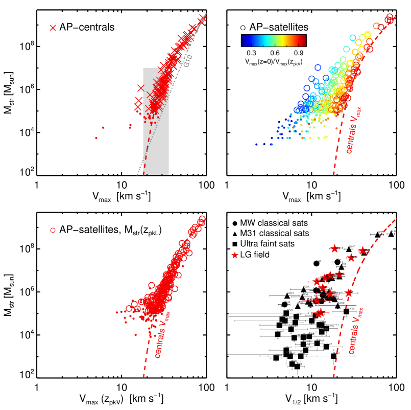
Figure 1: Top-left: Stellar mass, $M_{\rm str}$, versus maximum circular velocity, $V_{\rm max}$, of APOSTLE centrals. Crosses indicate all centrals $M_{\rm str}>10^{5}\,M_{\odot}$ (resolved with more than $\sim 10$ particles in AP-L1 runs); dots indicate systems with $M_{\rm str}<10^{5}\,M_{\odot}$ ($1$ to $10$ star particles). The dashed line is a fit of the form $M_{\rm str}/\,{\rm M}_{\odot}=m_{0}\,\nu^{\alpha}\exp(-\nu^{\gamma})$, where $\nu=V_{\rm max}/50\,{\rm km}\,\,{\rm s}^{-1}$, and $(m_{0},\alpha,\gamma)$ are $(3.0\times 10^{8},3.36,-2.4)$. The same dashed line is repeated in every panel for reference. The thin grey line shows the extrapolation to faint objects of the abundance-matching relation of Guo et al. (2010), also for reference. Top-right: Same as top left, but for APOSTLE satellites with $M_{\rm str}>10^{5}\,M_{\odot}$. Each satellite is coloured by the reduction in $V_{\rm max}$ caused by tidal effects. Bottom-left: As top-left, but for the ‘peak’ $M_{\rm str}$ and $V_{\rm max}$, typically measured just before first accretion into the primary halo. Bottom-right: $M_{\rm str}$ vs $V_{1/2}$ for LG dwarfs. Satellites of the MW and M31 are shown in black, ‘field’ objects are shown in red. Gas-rich disc galaxies such as the Magellanic Clouds, M 33, or IC 10, are not considered in our analysis.

3 The Simulations

The APOSTLE project consists of a suite of zoomed-in cosmological hydrodynamical simulations of $12$ volumes chosen to match the main dynamical characteristics of the LG. The full selection procedure is described in Fattahi et al. (2016) and a detailed discussion of the main simulation characteristics is given in Sawala et al. (2016b).

In brief, $12$ LG candidate volumes ware selected from the DOVE dark matter-only $\Lambda$CDM simulation of a periodic box $100\,{\rm Mpc}$ on a side (Jenkins, 2013). Each volume contains a relatively isolated pair of haloes with virial mass $M_{\rm 200}\sim 10^{12}\,{\rm M}_{\odot}$, separated by $d=600$–$1000$ kpc, and approaching each other with relative radial velocity in the range $V_{\rm rad}=0$–$250\,{\rm km}\,\,{\rm s}^{-1}$. The relative tangential velocity of the pair members was constrained to be less than $100\,{\rm km}\,\,{\rm s}^{-1}$, and the Hubble flow was constrained to match the small deceleration observed for distant LG members. Each zoomed-in volume is uncontaminated by massive boundary particles out to $\sim 3$ Mpc from the barycentre of the MW-M31 pair.

The candidate volumes were simulated at three different levels of resolution, labelled L1 (highest) to L3 (lowest resolution), using the code developed for the EAGLE project (Schaye et al., 2015; Crain et al., 2015). The code is a highly modified version of the Tree-PM/smoothed particle hydrodynamics code, P-Gadget3 (Springel, 2005). The hydrodynamical forces are calculated using the pressure-entropy formalism of Hopkins (2013), and the subgrid physics model was calibrated to reproduce the stellar mass function of galaxies at $z=0.1$ in the stellar mass range of $M_{\rm str}=10^{8}-10^{12}\,{\rm M}_{\odot}$, and to yield realistic galaxy sizes.

The galaxy formation subgrid model includes metallicity-dependent star formation and cooling, metal enrichment, stellar and supernova feedback, homogeneous X-ray/UV background radiation (hydrogen reionization assumed at $z_{\rm reion}=11.5$), supermassive black-hole formation, and AGN activity. Details of the subgrid models can be found in Schaye et al. (2015); Crain et al. (2015); Schaller et al. (2015b). The APOSTLE simulations adopt the parameters of the ‘ref’ EAGLE model in the language of the aforementioned papers.

Haloes and bound (sub)structures in the simulations are found using the FoF algorithm (Davis et al., 1985) and SUBFIND (Springel et al., 2001), respectively. First, FoF is run on the DM particles with linking length 0.2 times the mean inter particle separation to identify the haloes. Gas and star particles are then associated to their nearest DM particle. In a second step, SUBFIND searches iteratively for bound (sub)structures in any given FoF halo using all particle types associated to it. We shall refer to MW and M31 analogs as ‘primary’ or ‘host’ haloes, even though in some of the volumes they are found within the same FoF group. Galaxies formed in the most massive subhalo of each distinct FoF group will be referred to as ‘centrals’ or ‘field’ galaxies, hereafter.

Throughout this paper we use the highest resolution APOSTLE runs, L1, with gas particle mass of $\sim 10^{4}\,{\rm M}_{\odot}$ and maximum force softening length of $134$ pc. Four simulation volumes have so far been completed at resolution level L1, corresponding to AP-01, AP-04, AP-06, AP-11 in table 2 of Fattahi et al. (2016).

The simulations adopt cosmological parameters consistent with 7-year Wilkinson Microwave Anisotropy Probe (WMAP-7, Komatsu et al., 2011) measurements, as follows: $\Omega_{\rm M}=0.272$, $\Omega_{\Lambda}=0.728$, $h=0.704$, $\sigma_{8}=0.81$, $n_{s}=0.967$.

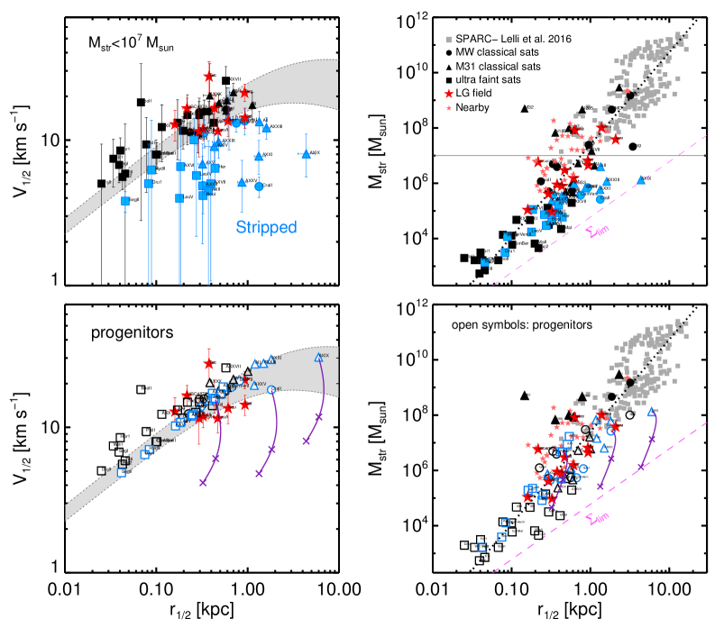
Figure 2: Top-left: Circular velocity, $V_{1/2}$, at the stellar half-mass radius, $r_{1/2}$, of LG ‘faint dwarfs’ ($M_{\rm str}<10^{7}\,{\rm M}_{\odot}$), as a function of $r_{1/2}$. The shaded area delineates the minimum velocities expected for such dwarfs, bracketed by two NFW profiles with $V_{\rm max}=20$ and $36\,{\rm km}\,\,{\rm s}^{-1}$, respectively (see shaded region in the top-left panel of Fig. 1; symbol types are as in the bottom-right panel of that figure). LG field dwarfs are shown in red, and are generally consistent with this expectation. Satellites with velocity dispersion below the shaded region are identified as having lost mass to tidal stripping, and are highlighted in cyan. Bottom-left: Same as top-left but for the progenitors of LG satellites, inferred as described in the text. The purple curves are three examples of ‘tidal stripping tracks’ (PNM08). Each tick mark corresponds to successive mass losses of $90$ per cent. The progenitor parameters are set by assuming that they match $M_{\rm str}$–$V_{\rm max}$ relation for isolated APOSTLE dwarfs, their $r_{1/2}$–$V_{1/2}$ follow CDM circular velocity profiles. (See Fig. 5 for a schematic description of the method.) Top-right: $M_{\rm str}$ vs $r_{1/2}$ relation for our galaxy sample as well as for the late-type galaxies in the SPARC survey (grey squares; Lelli et al., 2016a). The dashed magenta line roughly indicates the minimum effective surface brightness limit of current surveys. Bottom-right: Same as top-right, but for satellite progenitors. Note that the progenitors are in excellent agreement with other field galaxies, a result that provides independent support for our proposal that the low-velocity dispersion satellites identified as ‘stripped’ in the top-left panel have indeed been heavily affected by tidal stripping.

4 Results

4.1 Galaxy mass-halo mass relation in APOSTLE

The top-left panel of Fig. 1 shows the $M_{\rm str}$-$V_{\rm max}$ relation for all ‘central’ galaxies in the four L1 APOSTLE volumes. Since we are mainly interested in dwarfs, we only show galaxies forming in haloes with $V_{\rm max}<100\,{\rm km}\,\,{\rm s}^{-1}$ (or, roughly, $M_{\rm str}<10^{10}\,M_{\odot}$). Galaxy stellar masses are measured within the ‘galactic radius’, $r_{\rm gal}$, defined as $0.15\,r_{200}$.

This panel shows the tight relation between galaxy and halo masses anticipated for isolated APOSTLE galaxies in Sec. 1. Crosses indicate systems resolved with more than $10$ star particles, and small dots systems with $1$-$10$ star particles. It is clear that very few of the galaxies that succeed in forming stars in our AP-L1 simulations do so in haloes with $V_{\rm max}<20\,{\rm km}\,\,{\rm s}^{-1}$. In addition, essentially all isolated ‘faint dwarfs’ ($M_{\rm str}<10^{7}\,M_{\odot}$) inhabit haloes spanning a narrow range of circular velocity, $18<V_{\rm max}/\,{\rm km}\,\,{\rm s}^{-1}<36$. The few that stray to lower velocities are actually former satellites that have been pushed out of the virial boundaries of their primary halo by many-body interactions (Sales et al., 2007; Ludlow et al., 2009; Knebe et al., 2011).

The top-right panel of Fig. 1 is analogous to the top-left, but for ‘satellite’ galaxies , defined as those within 300 kpc of either primary. The difference with isolated systems is obvious: at fixed $M_{\rm str}$ the haloes of satellite galaxies can have substantially lower $V_{\rm max}$ than centrals (see, also, Sawala et al., 2016a).

The difference is almost entirely due to the effect of tides experienced by satellites as they orbit the potential of their hosts. This is clear from the bottom-left panel of Fig. 1, which shows the same relation for satellites, but for their ‘peak’ $M_{\rm str}$ and $V_{\rm max}$, which typically occur just before a satellite first crosses the virial boundary of its host. At that time, the satellite progenitors followed a $M_{\rm str}$-$V_{\rm max}$ relation quite similar to that of isolated dwarfs.

Finally, the bottom-right panel of Fig. 1 shows the stellar mass-circular velocity relation for LG dwarfs, where the colours distinguish satellites (black) from field or isolated systems (shown in red). This panel differs from the others because the maximum circular velocity is not accessible to observation; therefore, we show instead $V_{1/2}$, the circular velocity at the half-mass radius (see Eq. 2).

The results shown in Fig. 1 elicit a couple of comments. One is that all LG dwarfs lie to the left of the red dashed line that delineates the $M_{\rm str}$-$V_{\rm max}$ relation for field APOSTLE dwarfs. This is encouraging, since consistency with our model demands $V_{1/2}<V_{\rm max}$ for all dark matter-dominated dwarfs. (The only exception is M32, a compact elliptical galaxy whose internal dynamics are dictated largely by its stellar component.)

Second, aside from a horizontal shift, the general mass-velocity trend of LG dwarfs is similar to that in the simulations: below a certain stellar mass, the characteristic velocities of LG dwarfs become essentially independent of mass, just as for their simulated counterparts.

Finally, note that we do not show measurements of $V_{1/2}$ for APOSTLE galaxies in Fig. 1. This is mainly because of the limited mass and spatial resolution of the simulations. The majority of the LG satellites have stellar masses below $10^{6}\,{\rm M}_{\odot}$, which are resolved with fewer than $100$ stellar particles in even the best APOSTLE runs, thus compromising estimates of their half-mass radii and velocity dispersions. In addition, at very low masses, all APOSTLE galaxies have similar, resolution-dependent, half-mass radii, a clear artefact of limited resolution. Indeed, most AP-L1 dwarfs with $M_{\rm str}<10^{6}\,M_{\odot}$ have $R_{\rm eff}\sim 400$ pc (Campbell et al., 2016). This is far in excess of the typical radii of LG dwarfs of comparable mass, compromising direct comparisons between the observed and simulated stellar velocity dispersions and radii of faint dwarfs.

We shall therefore adopt an indirect, but more robust, approach, where we assume that the stellar mass-halo mass APOSTLE relation is reliable and use it, together with the known mass profile of CDM haloes, to interpret various observational trends in the structural parameters of Local Group dwarfs. Our analysis thus rests on two basic assumptions: (i) that the $M_{\rm str}$-$V_{\rm max}$ relation of field dwarfs follows roughly that shown in the top-left panel of Fig. 1; and (ii) that the baryonic assembly of the galaxy does not alter dramatically the inner dark mass distribution.

The first assumption imposes a fairly sharp halo mass ‘threshold’ for galaxy formation, as seen in the top-left panel of Fig. 1. The existence of this threshold has been critically appraised by recent work, some of which argues that halos with masses well below the threshold may form luminous galaxies (Wise et al., 2014; O’Shea et al., 2015), some as massive as the Cra 2 or Draco dwarf spheroidals (see, e.g., Ricotti et al., 2016). We note, however, that those simulations are typically stopped at high redshift ($z\sim 8$) and rarely followed to $z=0$, so it is unclear whether the threshold they imply (if expressed in present-day masses) is inconsistent with the one we assume here. Indeed, the latest simulation work, which includes a more sophisticated treatment of cooling than ours and follows galaxies to $z=0$, reports a comparable ‘threshold’ to the one we use here (Fitts et al., 2017).

Regarding the second assumption, we emphasize that this is a conservative one, since baryon-induced cores would only help to reconcile CDM theoretical expectations with observations.

Figure 3: Top: Tidally-induced changes in the stellar half-mass radius ($r_{1/2}$) and stellar velocity dispersion ($\sigma$), as a function of the total mass that remains bound within the original stellar half-mass radius of the galaxy. The parameters are in units of their pre-stripping values. Thick dotted lines correspond to the models of Errani et al. (2015) for spheroidal galaxies embedded in cuspy CDM haloes. The thin solid lines indicate results for all APOSTLE satellites with $M_{\rm str}>10^{6}\,{\rm M}_{\odot}$ at present time. We also show, with dot-dashed lines, APOSTLE satellites with $z=0$ stellar masses in the range $10^{5}-10^{6}\,{\rm M}_{\odot}$ who have lost more than 90 per cent of their stellar mass in the past. Bottom: Similar to the top panel but for changes in the stellar mass ($M_{\rm str}$) and gas mass ($M_{\rm gas}$), both given in units of the pre-stripping stellar mass.

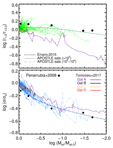
Figure 4: Tidally-induced changes in half-mass radius ($r_{1/2}$, top panel), and stellar velocity dispersion ($\sigma$, bottom panel), as a function of the remaining bound fraction of stellar mass. All parameters are in units of their pre-stripping values. Line types are as in Fig. 3. Thick dotted curves are E15 tidal tracks; thin solid and dot-dashed lines are results for APOSTLE satellites, as in Fig. 3. Solid circles coresspond to the six models of PNM08 at the end of their simulations. Thin solid lines of different colors show results for four disc dwarfs simulated by Tomozeiu et al. (2016). See text for further discussion.

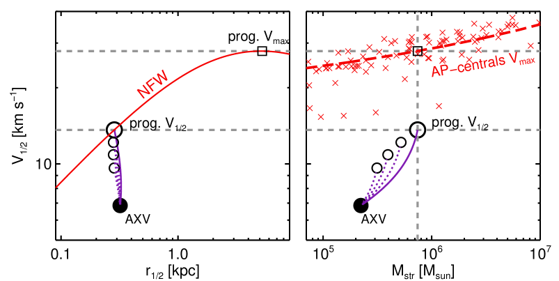
Figure 5: A schematic example to illustrate how we determine the properties of the progenitors of satellites deemed ‘stripped’ (cyan symbols in the top-left panel of Fig. 2). The example applies to And XV, whose present-day half-mass radius, circular velocity, and stellar mass are indicated by the solid circle. The E15 tidal tracks suggest a number of possible progenitors, shown by open circles. The actual And XV progenitor (open square in the right-hand panel) is selected to match simultaneously the APOSTLE $M_{\rm str}$-$V_{\rm max}$ relation for isolated dwarfs, and the circular velocity $V_{1/2}$ at $r_{1/2}$ expected for a CDM halo of that $V_{\rm max}$ (large open circle in left-hand panel).

4.2 Tidal stripping effects on LG satellites

4.2.1 Size-velocity relation

One firm prediction of our simulations is that all dwarfs with $M_{\rm str}<10^{7}\,M_{\odot}$ should form in haloes of similar mass. Because the inner circular velocity profile of CDM haloes increases with radius, we expect the dark matter content of dwarfs to increase with galaxy size, as larger galaxies should encompass larger amounts of dark matter. This implies that a ‘minimum’ velocity can be predicted for a faint dwarf, based solely on the dark mass contained within its half-mass radius. This is indicated by the grey shaded region in the top-left panel of Fig. 2, which indicates the dark matter circular velocity profiles expected for haloes close to the ’threshold’ (i.e., $18<V_{\rm max}/\,{\rm km}\,\,{\rm s}^{-1}<36$), modeled as NFW haloes with concentrations taken from Ludlow et al. (2016).

As is clear from this panel, a number of dwarfs are at odds with this prediction, and are highlighted in cyan. Note that all of these deviant systems are satellites (field dwarfs are shown in red). Within the constraints of our model the only way to explain the low velocity dispersion of these systems is to assume that they have been affected by tides. Extreme examples include Cra 2 and And XIX; i.e., systems with large half-light radii and very low velocity dispersions that are otherwise difficult to explain in our model.

4.2.2 The progenitors of stripped satellites

The effects of tides on dark matter-dominated spheroidal systems deeply embedded in NFW haloes have been explored in detail by PNM08 and E15. One of the highlights of these studies is that structural changes in the stellar component depend solely on the total amount of mass lost from within the original stellar half-mass radius of a galaxy. The fraction of stellar mass that remains bound, the decline in its velocity dispersion, and the change in its half-mass radius are thus all linked by a single parameter, implying that a tidally-induced change in one of these parameters is accompanied by a predictable change in the others.

In other words, tidally stripped galaxies trace prescribed tracks in the space of $M_{\rm str}$, $V_{1/2}$, and $r_{1/2}$ variables. This restricts the parameter space that may be occupied by stripped galaxies once the mass-size-velocity scaling relations of the progenitors are specified.

The PNM08, or E15, ‘tidal tracks’ may be summarized by a simple empirical formula that describes parametrically the tidal evolution of any such structural parameter, referred generically as $h$, in units of the original value, for a spheroidal system deeply embedded in a cuspy (NFW) CDM halo:

$$h(x)={2^{\alpha}\,x^{\beta}\over(1+x)^{\alpha}}.$$ (3)

Here the parameter $x$ is the total mass ($M_{\rm h}$) that remains bound within the initial stellar half-mass radius of the dwarf, in units of the pre-stripping value. The values of $\alpha$ and $\beta$ are taken from E15 and given, for each structural parameter, in Table 1.

Table 1: Tidal evolutionary tracks according to Errani et al. (2015)

		$M_{\rm str}/M_{\rm str,0}$	$\sigma/\sigma_{0}$	$r_{1/2}/r_{1/2,0}$
$\alpha$		3.57	-0.68	1.22
$\beta$		2.06	0.26	0.33

We show these tidal tracks in Fig. 3 as thick dotted lines, for the case of the half-mass radius and velocity dispersion (top panel) and stellar mass (bottom). The tracks indicate that a spheroidal galaxy that loses $\sim 90$ per cent of its original stellar mass is expected to experience a reduction of a factor of $\sim 2.5$ in its velocity dispersion. On the other hand, its half-mass radius would change by less than $20\%$. To first order, then, even if tides are able to reduce substantially $M_{\rm str}$ and $\sigma$, they are expected to have little effect on the size of an NFW-embedded dwarf spheroidal.

The thin lines in Fig. 3 show that the same tidal tracks describe rather well the the change in $r_{1/2}$, $M_{\rm str}$, and $\sigma$ of APOSTLE satellites since they first cross the virial radius of their host halo. The E15 or PNM08 models do not include star formation, so we only consider in the comparison star particles born before infall. We show all APOSTLE satellites with $z=0$ stellar masses exceeding $10^{6}\,{\rm M}_{\odot}$ (these satellites are resolved with at least $1000$ star particles at $z=0$), as well as those with stellar masses in the range $10^{5}-10^{6}\,{\rm M}_{\odot}$ who have lost 90 per cent of their stellar mass since infall.

The agreement between the E15 models and APOSTLE satellites shown in Fig. 3 is remarkable, especially considering that most APOSTLE dwarfs are gas-rich at first infall, with gas-to-star mass ratios of order 10 to 30, and that the tidal tracks are only meant to decribe the evolution of the stellar component. Indeed, the gas component is lost quickly after infall as a result of tides and ram-pressure in the host halo (Arraki et al., 2014; Frings et al., 2017), as shown by the thin grey lines in the bottom panel of Fig. 3. The gas mass loss, however, has little influence on the evolution of the stellar component, which remains close to the tidal tracks. This is because baryons never dominate the gravitational potential of APOSTLE dwarfs; the only parameter that determines the tidal evolution is the change in total mass, which is therefore mostly dark. The results we describe below, therefore, apply mainly to dark matter-dominated dwarf spheroidals, and might need revision when considering systems where baryons dominate, such as, e.g., M32, or systems where most stars are in a thin, rotationally-supported disc (see, e.g., Tomozeiu et al., 2016).

Since the changes in stellar mass, velocity dispersion, and half-mass radius depend on a single parameter, this implies that they can be expressed as a function of each other. This is shown in Fig. 4, which shows the same tracks as in Fig. 3, but expressed as a function of the remaining fraction of bound stars. Here the E15 tidal tracks corresponding to spheroidals embedded in cuspy DM haloes (thick dotted lines) are compared with APOSTLE results (thin lines), as well as with those of PNM08 (filled circles), and with those of Gal A-D from Tomozeiu et al. (2016, see legend). The latter authors embed a thin exponential disc of stars, rather than a spheroid, in a cuspy halo. The E15 tracks in general reproduce well the tidally-induced evolution of a dwarf, except perhaps for Gal A of Tomozeiu et al. (2016), which deviates from the E15 radius track when the stellar mass loss is extreme (i.e., more than 90 per cent). We note, however, that the few APOSTLE dwarfs who suffer comparable stellar mass loss seem to agree with the E15 tracks quite well. The difference is likely due to the fact that the initial galaxies in Tomozeiu et al. (2016) are pure exponential discs rather than spheroids, but further simulations would be needed to confirm this.

One important corollary of these results is that the E15 tidal tracks can be used to ‘undo’ the effects of stripping once the structural properties of the progenitors are specified. We attempt this in the bottom-left panel of Fig. 2, where we show the $V_{1/2}$ vs $r_{1/2}$ relation for the progenitors of all LG satellites, assuming that they follow the APOSTLE scaling relations appropriate for isolated dwarfs (i.e., top-left panel of Fig. 1).

A detailed, schematic example of the procedure is presented in Fig. 5 for the case of And XV: the properties of the progenitor are uniquely specified once it is constrained to match simultaneously the $M_{\rm str}$–$V_{\rm max}$ relation expected of APOSTLE isolated dwarfs and the $r_{1/2}$–$V_{1/2}$ relation, assuming NFW mass profiles. ‘Progenitors’ computed this way will be shown with open symbols in subsequent figures. The parameters of LG satellites and their assumed progenitors are listed in Tables LABEL:TabData2 and LABEL:TabProg.

The tracks in the bottom-left panel of Fig. 2 highlight three systems which, according to our procedure, have been very heavily stripped: Cra 2, And XIX, and Boo I. A tickmark along each track indicates successive factors of $10$ in stellar mass loss. For most satellites the procedure suggests modest mass losses, but for these three (rather extreme) examples our procedure suggests that each has lost roughly $99$ per cent of their original mass.

4.2.3 Mass-size relation

The discussion above suggests that tides have had non-negligible effects on many LG satellites. Is there any independent supporting evidence for this conclusion? One possibility is to examine how other scaling laws are affected by the changes in velocity and radius prescribed by our progenitor-finding procedure. We emphasize that this procedure is based on a single assumption (aside from assuming NFW mass profiles for the progenitors): that all satellites descend from progenitors that follow the $M_{\rm str}$-$V_{\rm max}$ relation for isolated dwarfs in APOSTLE.

We begin by examining, in the top-right panel of Fig. 2, the stellar mass versus half-light radius relation for our whole galaxy sample, enlarged by the late-type galaxies from the SPARC sample of Lelli et al. (2016a). Galaxy size and mass are clearly correlated ($M\propto r^{2/7}$; thick dotted line), so that the effective surface brightness increases roughly as $\Sigma\propto M^{3/7}$. There is also substantial scatter in radii at fixed stellar mass, and vice versa.

An interesting feature of this plot is the clear separation between the satellites deemed ‘stripped’ because of their low velocity dispersion (shown in cyan) and field LG dwarfs (shown in red). Although there is little overlap in stellar mass, satellites and field LG dwarfs do overlap in size. Satellites, however, appear to follow a different trend in the mass-radius plane than that of the general population (shown with a dashed line in the top-right panel of Fig. 2. In our interpretation, this difference in mass at fixed radius is a signature of tidal stripping, and should disappear when considering the properties of their progenitors.

We show this in the bottom-right panel of Fig. 2, where we can see that the mass and size of the progenitors are in excellent agreement with the general population of field galaxies. In other words, the same correction in velocity dispersion required to restore agreement with APOSTLE predictions for isolated dwarfs also brings the population of ‘stripped’ satellites into agreement with the general field population in terms of stellar mass and size. We emphasize that there is no extra freedom in this procedure. Once the change in velocity dispersion is specified, the change in radius and mass follows, as illustrated by the stripping tracks in Fig. 3.

This exercise offers a simple explanation for why satellites as faint and kinematically cold as Cra 2 and And XIX are so large in size: they are the tidal descendants of once more massive systems, which were born physically large and have remained so even after being heavily stripped. Recall that, according to the stripping tracks of PNM08 and E15, the size of the stellar component of a dSph embedded in an NFW halo is affected little by stripping, even after losing $\sim 99$ per cent of its original stellar mass.

Note as well that not all satellites are strongly stripped, and that those that have been stripped have been affected to varying degrees. This is not unexpected, since the effectiveness of stripping depends sensitively on the mass of the satellite; on how concentrated the stellar component is within its halo; on the pericentric distance of its orbit; and on the number of orbits it has completed. All of those parameters can vary widely from system to system, scrambling the original $r_{1/2}$-$V_{1/2}$ correlation (bottom-left panel of Fig. 2) and turning into the largely scatter plot we see in the top-left panel of the same figure.

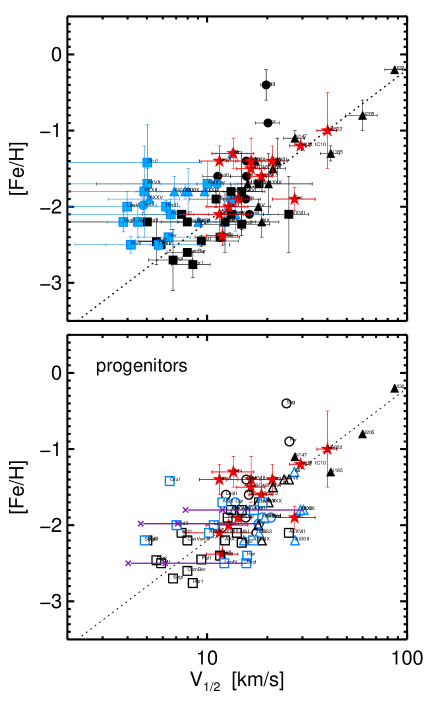
Figure 6: Top: [Fe/H] vs $V_{1/2}$ for dwarf galaxies in the LG. Symbol types and colours are as in Fig. 2. The stripped satellites (cyan symbols), contribute a population that flattens the relation at the low-velocity end. Satellites deemed ‘stripped’ have lower velocity dispersions than field dwarfs (red symbols) of comparable metallicity. Bottom: As top panel, but for satellite progenitors, assuming that their metallicities are unaffected by tides (i.e., they shift only horizontally in this plot). The tidal stripping correction restores agreement between satellites and field galaxies, and result in a tighter, monotonic relation between metallicity and velocity for all dwarfs.

4.2.4 Metallicity-velocity dispersion relation

Tidal stripping is expected to affect the least scaling laws involving the metallicity of a dwarf, which would only be modified in the case of a pronounced metallicity gradient in the progenitor. Assuming, for simplicity, that tidal losses leave the average metallicity of a satellite unchanged, we examine the effects of stripping on the relation between metallicity and velocity dispersion. We prefer to use velocity dispersion instead of stellar mass because, according to the tidal tracks of E15 or PNM08, changes in velocity are a more sensitive measure of tidal stripping than changes in stellar mass.

This is shown in the top panel of Fig. 6 for all galaxies in our sample (Sec. 2.2) with published measurements of these two quantities. We use in this panel the latest observed metallicities, but caution that some are estimated spectroscopically from individual stars whereas others rely on photometric estimates based on the color of the red giant branch (see McConnachie, 2012, and references therein). There is a reasonably well defined trend of increasing metallicity, [Fe/H], with increasing $V_{1/2}$, except at the low velocity end, where the trend falters and the relation turns flat.

The flattening is largely a result of the low-velocity population that we have identified as ‘stripped’ satellites (shown in blue in Fig. 6). Interestingly, the trend between velocity and metallicity for progenitors is monotonic and tighter when considering their inferred progenitors (bottom panel of the same figure), lending further support to our assumption that the low-$V_{1/2}$ population originates from tides.

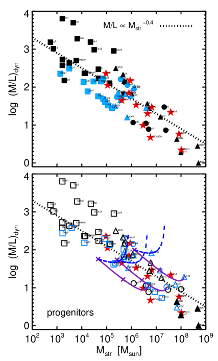
Figure 7: As Fig. 6, but for the stellar mass vs dynamical mass-to-light ratio relation. The top panel shows the results for LG dwarfs; bottom panel for their inferred progenitors. Note that tidal stripping moves satellites along tracks parallel to the observed relation, so that stripped and unstripped systems follow the same relation. The thick dotted lines show $(M/L)_{\rm dyn}\propto M^{-0.4}$, motivated by the $V\propto r^{1/2}$ relation expected for the inner regions of an NFW halo, together with the $L\propto r^{7/2}$ scaling that holds for field galaxies (see top-right panel of Fig. 2). The blue dashed lines represent tidal tracks for a model in which the dark matter halo has a central core of size comparable to the size of the corresponding stellar component.

4.2.5 Dynamical mass-to-light ratios

One firmly established dwarf galaxy scaling law links the dynamical mass-to-light ratio, $(M/L)_{\rm dyn}\equiv M_{1/2}/(L_{V}/2)$, with the total luminosity. As discussed in the early review by Mateo (1998), dSphs have mass-to-light ratios that increase markedly with decreasing luminosity, ‘consistent with the idea that each is embedded in a dark halo of fixed mass’. How is this relation modified by our proposal that tidal stripping may have altered the size, stellar mass, and velocity dispersion of many satellites?

We examine this in Fig. 7, where the top panel shows the dynamical mass-to-light ratios of all LG galaxies in our sample, as a function of stellar mass. Interestingly, tidal stripping does not alter this overall scaling, as it mainly shifts galaxies along lines roughly parallel to the main trend. Indeed, the progenitors sample a very similar relation as the present-day satellites, as may be seen in the bottom panel of Fig. 7. As discussed by PNM08, this is a result of the particular tidal stripping tracks expected for stellar systems embedded in ‘cuspy’ NFW haloes.

If dark matter haloes had instead constant density cores comparable in size to the stellar component, then the change in mass-to-light ratio due to tidal stripping for a given change in stellar mass would be much more pronounced. This is shown by the blue dashed lines, which indicate the tidal tracks expected in such a case, as given by E15. Had some satellites lost a large fraction of their original mass to tides, they would have moved away from the $(M/L)_{\rm dyn}$-$M_{\rm str}$ relation that holds for the progenitors. On the other hand, if haloes are ‘cuspy’ then tidally-stripped galaxies just move along the observed relation: isolated dwarfs, progenitors, and tidal remnants are all expected to follow the same relation.

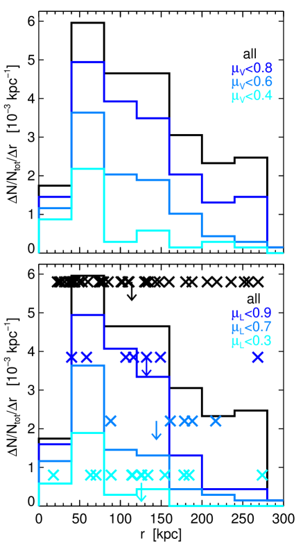
Figure 8: Top: Radial distribution of all APOSTLE satellites with $M_{\rm str}>10^{5}\,M_{\odot}$ (black curves). Lower coloured histograms correspond to ‘stripped’ systems, as estimated by the parameter $\mu_{\rm v}$, which measures the decline in $V_{\rm max}$ caused by tides (see text for details). Bottom: Same as top, but for the stripping parameter $\mu_{\rm L}$, which measures the loss in stellar mass caused by tides. Note that highy stripped systems are more centrally concentrated than the average satellite population. Crosses indicate the location of LG satellites, coloured by their inferred tidal mass loss, as described in Sec. 4.2.2, and summarized in Table LABEL:TabProg. See text for further discussion.

4.2.6 Tidal stripping and satellite shapes

Our discussion above suggests that the observed dwarf galaxy scaling laws pose no fundamental problem to a scenario where tides have affected a number of satellites, even if in some cases, such as Cra 2 and And XIX, the posited fraction of mass lost may approach $99$ per cent. Two oft-cited arguments against this scenario involve satellite shapes and their distances to the primary galaxy.

Cra 2, for example, is rather round on the sky, and it is today situated at $\sim 115$ kpc from the Galactic Centre (Torrealba et al., 2016). Do such observations contradict our idea that Cra 2 has lost many of its original stars to tides?

Not necessarily. First, we should recall that the idea that heavily stripped systems must be very aspherical only applies to systems near the pericentre of their orbits and thus ‘caught in the act’ of being stripped, such as, for example, the Sagittarius dSph (Ibata et al., 2001; Majewski et al., 2003), and the globular cluster Pal 5 (Odenkirchen et al., 2001, 2003). These are clearly convincing examples of the effect of Galactic tides, but not typical.

Indeed, we expect most satellites to be on rather eccentric orbits around the Galactic Centre, which means that tidal effects are best approximated as impulsive perturbations that operate at pericentre. As discussed by Peñarrubia et al. (2009), the signature of Galactic tides fades away from the bound remnant quickly (i.e., within one crossing time) after pericentric passage. This implies that the effect of tides is actually rather difficult to discern when the satellite is at apocentre, where it spends most of its orbital time and is therefore most likely to be found.

In addition, tidal remnants are expected to be much rounder than their progenitors when equilibrium has been restored (see; e.g., Barber et al., 2015, and references therein). Tides actually tend to reduce the original asphericity of a galaxy, implying that there is in principle no contradiction between round satellite shapes and the possibility of heavy tidal stripping.

4.2.7 Tidal stripping and satellite spatial distribution

Satellites that have been extremely affected by tides are expected to be in orbits with small pericentric distances and should have completed at least a few orbits around the primary galaxy. The latter condition implies either a small apocentre or an early time of accretion into the primary halo, or both. One may therefore argue that the large distances from the Galactic Centre of some low velocity dispersion satellites are inconsistent with a tidal origin for their peculiar properties.

We examine this in APOSTLE, where we can easily identify systems that have experienced substantial tidal mass loss, track their orbits, and compute their orbital parameters. We explore two alternative measures of tidal stripping for subhaloes that, at $z=0$, still host a luminous satellite: one is the reduction in $V_{\rm max}$ experienced since accretion; the other is the stellar mass loss since the peak of stellar mass.

Neither measure is ideal. The first one suffers from the fact that $V_{\rm max}$ changes are sensitive mostly to the tidal loss of dark matter, which couples in a complex and indirect way to actual stellar mass losses. The second quantity measures directly stellar mass losses but is vulnerable to numerical artefact, since the mass loss is expected to depend sensitively on the stellar half-mass radii, which are poorly resolved in APOSTLE, especially at the faint end (see discussion in Sec. 4.1).

We therefore pursue both alternatives in our analysis, and show the results in Fig. 8. Because of the caveats above, this is only meant to identify possible major inconsistencies in our argument, rather than to provide quantitative estimates that can be directly compared with observations.

The top panel of Fig. 8 shows, in black, the radial distribution of all $M_{\rm str}>10^{5}\,M_{\odot}$ satellites found, at $z=0$, within $300$ kpc from the centre of AP-L1 primaries. The luminous satellite radial distribution is also shown for several subsamples, drawn according to the tidally-induced reduction of the maximum circular velocity of each subhalo, measured by the ratio $\mu_{\rm v}=V_{\rm max}(z=0)/V_{\rm max}(z_{\rm pkV})$. Here $z_{\rm pkV}$ identifies the time when $V_{\rm max}$ peaked, which typically occurs just before being first accreted into the primary halo.

The various distributions in the top panel of Fig. 8 (labelled by $\mu_{\rm v}$) show the radial segregation of satellites that have been heavily affected by tides. Clearly, the larger the effects of tides, the closer to the galaxy centre satellites lie, on average. Note that heavily stripped systems are not particularly rare: $18$ per cent of all subhaloes with satellites as massive as $M_{\rm str}>10^{5}\,M_{\odot}$ have $\mu_{\rm v}<0.4$. This corresponds to a rather large ($>95$ per cent) loss of the original total bound mass (see PNM08’s Fig. 8). Note that some of these very highly stripped objects may be found quite far from the centre of the primary, even as far out as $\sim 250$ kpc.

The bottom panel of Fig. 8 is analogous to that in the top, but adopting the ratio $\mu_{\rm L}=M_{\rm str}(z=0)/M_{\rm str}(z_{\rm pkL})$. Here $z_{\rm pkL}$ identifies the time when the stellar mass of a satellite peaked. The various distributions, labelled by the corresponding values of $\mu_{\rm L}$, show that heavily stripped systems are not particularly rare. Of all surviving luminous satellites in APOSTLE, more than $13$ per cent have lost $>70$ per cent of their stars (i.e., $\mu_{\rm L}<0.3$), but we caution again that this number is rather uncertain because of limited resolution. The sequence of histograms in the right panel of Fig. 8 again shows that highly stripped satellites tend to be more centrally concentrated than the average.

We compare this with our stripping estimates for the LG satellite population by indicating with crosses the distance to the primary (MW or M31) of all satellites (in black) and of those deemed, according to our progenitor-finding procedure, to have lost various fractions of their original mass (in colour; each satellite is only plotted once, and the median of each population is shown with a small arrow).

Focusing on the most highly-stripped population (i.e., $\mu_{\rm L}<0.3$) we note that most of them are well within $150$ kpc of the centre, both in the observations and in the simulations. We conclude that there is no obvious inconsistency between the spatial distribution of low-velocity dispersion satellites and our hypothesis that their peculiar properties have been caused by tidal stripping.

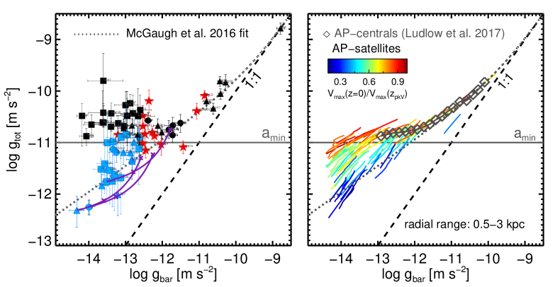
Figure 9: Left: The acceleration, $g_{\rm tot}=V_{1/2}^{2}/r_{1/2}$, at the stellar half-mass radius, as a function of the baryonic contribution at that radius, $g_{\rm bar}=GM_{\rm str}/2\,r_{1/2}^{2}$, computed assuming spherical symmetry. The symbols show results for all LG dwarfs, using the same colours and types as in Fig. 2. The thick dotted line is the empirical MDAR fit of McGaugh et al. (2016), as given by Eq. 4. The horizontal line highlights $a_{\rm min}$, the minimum acceleration expected for isolated dwarfs in $\Lambda$CDM (Navarro et al., 2016). Tidal stripping is expected to push some satellites below that minimum, as shown by the tidal tracks shown in magenta. Note the large scatter at the low-$g_{\rm bar}$ end. Right: As left panel but for the average of all APOSTLE central (‘field’) galaxies (connected squares, as given by Ludlow et al., 2017). Coloured red lines illustrate the expected location of APOSTLE satellites in this panel. Since the stellar half-mass radii of faint simulated satellites is poorly constrained, we show for each subhalo a line segment that spans a wide range in radius, $0.5<r/{\rm kpc}<3$, covering the full observed range in $r_{1/2}$ at given $M_{\rm str}$. Each subhalo is coloured by the tidal stripping measure $\mu_{\rm v}$ introduced in Sec. 4.2.7, which measures the decline in $V_{\rm max}$ caused by stripping. Note that satellites are expected to ‘fan out’ at low values of $g_{\rm bar}$, as observed in the left-hand panel.

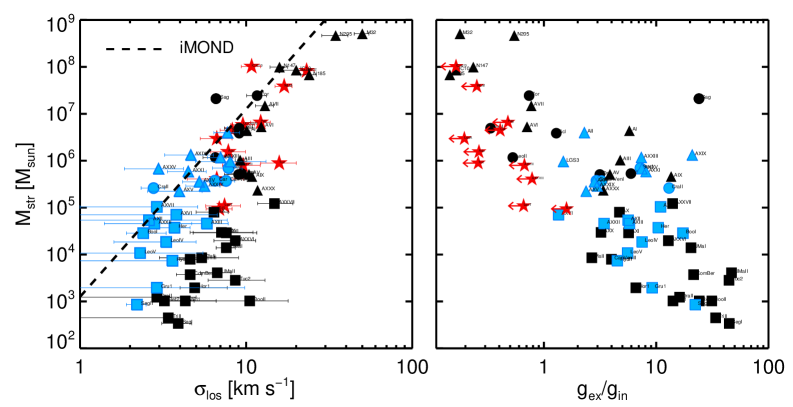
Figure 10: Left: Stellar mass-velocity dispersion relation for all LG dwarfs. Symbols and and colours are as in Fig. 2. The thick dotted line is the MOND prediction for isolated systems, as in Eq. 6. Note that many faint galaxies have velocity dispersions well in excess of what is predicted by MOND. Right: Stellar mass as a function of the ratio of ‘external’ to ‘internal’ accelerations, $g_{\rm ex}/g_{\rm in}$. This provides a measure of the importance of ‘external field effects’ (EFE) on MOND predictions.

4.3 Tidal stripping and the MDAR

One consequence of the effects of tidal stripping discussed in the previous subsection is that stripping is expected to scatter satellite galaxies away from the ‘mass discrepancy-acceleration relation’ (MDAR) that holds for isolated galaxies. Various forms of this relation have been proposed in the past, but we adopt for our discussion here the latest results of McGaugh et al. (2016) and Lelli et al. (2016a).

These authors show a tight correlation between the gravitational acceleration estimated from the rotation curve of late-type galaxies, $g_{\rm tot}=V_{\rm rot}^{2}(r)/r$, and the acceleration expected from the luminous (baryonic) component of a galaxy, $g_{\rm bar}=V_{\rm bar}^{2}(r)/r$, where $V_{\rm bar}(r)$ is the contribution of the baryons to the circular velocity at radius $r$. The relation may be approximated by the fitting function,

$$g_{\rm tot}={g_{\rm bar}\over 1-e^{-\sqrt{g_{\rm bar}/g_{\tau}}}}\,,$$ (4)

over the range $-11.7<\log(g_{\rm bar}/{\rm m\,s}^{-2})<-9$, with relatively small residuals.

At the (faint) low-$g_{\rm bar}$ end, the relation seems to flatten, with $g_{\rm tot}$ approaching an asymptotic minimum value of $a_{\rm min}\sim 10^{-11}{\rm m\,s}^{-2}$ (Lelli et al., 2016b). This flattening has been called into question by the Cra 2 dSph, which seems to lie on the extrapolation of Eq. 4 (McGaugh, 2016), at $(g_{\rm bar},g_{\rm tot})=(1.0\times 10^{-14},5.6\times 10^{-13})$, with all accelerations measured in ${\rm m\,s}^{-2}$.

This issue is of interest to our discussion, since $\Lambda$CDM dwarf galaxy formation models such as that of APOSTLE make a very specific prediction for this relation: the minimum halo mass threshold discussed in Sec. 4.1 to host a luminous dwarf translates into a well-defined minimum acceleration that all isolated dwarfs must satisfy. As discussed in detail by Navarro et al. (2016) and Ludlow et al. (2017), this minimum acceleration is of order $a_{\rm min}\sim 10^{-11}{\rm\,m\,s}^{-2}$, which provides a natural and compelling explanation for the faint-end flattening of the relation reported by Lelli et al. (2016b).

We illustrate the simulation predictions in the right-hand panel of Fig. 9, where the connected open squares indicate the median $g_{\rm bar}$-$g_{\rm tot}$ relation for all APOSTLE centrals. The thick dotted line follows Eq. 4, and it is clear from the comparison that isolated APOSTLE galaxies follow a very similar relation to the observed one, at least for $g_{\rm bar}>10^{-12}{\rm\,m\,s}^{-2}$. At lower $g_{\rm bar}$ the total accelerations of APOSTLE centrals approach $a_{\rm min}$.

Tidal stripping is expected to modify this relation, reducing $g_{\rm bar}$ and shifting satellites to $g_{\rm tot}$ values well below $a_{\rm min}$. This is illustrated by the coloured lines in the right panel of Fig. 9, which indicate where faint dwarfs affected by tidal stripping would be expected to lie, depending on their half-mass radius. Satellites affected little by stripping (shown in red) are expected to continue the flattening trend, whereas heavily stripped satellites should fall below the $a_{\rm min}$ boundary, and approach, in extreme cases (shown in blue), the extrapolation of Eq. 4 (dotted line).

A simple and robust prediction from APOSTLE-like models is then that tidal stripping should scatter satellites below the mean $g_{\rm bar}$-$g_{\rm tot}$ trend that holds for isolated systems, leading to substantial spread in the value of $g_{\rm tot}$ at fixed $g_{\rm bar}$ at the faint end.

This is, indeed, what is observed in the observational data for LG satellite and field dwarfs. We show this in the left-hand panel of Fig. 9, using for $g_{\rm tot}$ and $g_{\rm bar}$ the values estimated at the half-mass radius, assuming spherical symmetry for both the dark matter and baryonic components, or, more specifically,

$$g_{\rm tot}=V_{1/2}^{2}/r_{1/2},\quad g_{\rm bar}=G\,M_{\rm str}/2\,r_{1/2}^{2}$$ (5)

The data in this panel show that the tight MDAR reported by McGaugh et al. (2016) and Lelli et al. (2016b) for brighter galaxies breaks down in the very faint, low-surface brightness regime ($g_{\rm bar}<10^{-12}{\rm m\,s}^{-2}$). The scatter in $g_{\rm tot}$ at given $g_{bar}$ spreads nearly two decades, seriously calling into question the idea that MDAR might encode a ‘natural law’ that allows the total gravitational acceleration to be accurately estimated from the baryonic contribution alone.

The observed data, on the other hand, are quite consistent with the APOSTLE predictions, once the effects of tidal stripping are taken into account. Interestingly, our models predict that the most heavily tidally stripped satellites should approach the extrapolation of Eq. 4. (Cra 2 is one example of several in that regard.) On the other hand, those largely unaffected by tides should hover just above the $g_{\rm tot}=a_{\rm min}$ line, as observed. More moderately stripped systems should bridge the gap between the two, just as observed in the left-hand panel of Fig. 9.

We conclude that the overall behaviour of dwarf satellites galaxies in the $g_{\rm obs}$ vs $g_{\rm bar}$ plane can be understood in the $\Lambda$CDM framework as a simple consequence of tidal stripping.

4.4 MOND and the velocity dispersion of LG dwarfs

The extremely low accelerations of faint dwarfs lie in the regime where the modified Newtonian gravity theory MOND (Milgrom, 1983) makes definite and clear predictions—the ‘deep-MOND limit’. In this regime, the characteristic velocity of a non-rotating stellar spheroid is determined solely by its mass (equal to that of the stellar component in the case of a dSph) and by the MOND acceleration parameter, $a_{0}=1.2\times 10^{-10}{\rm m\,s}^{-2}=3.7\times 10^{3}{\rm\,km}^{2}{\rm\,s}^{-2}{\rm\,kpc}^{-1}$ (Milgrom, 2012).

Following McGaugh & Milgrom (2013), the MOND velocity dispersion may be written as:

$$\sigma_{\rm iMOND}=(4GM_{\rm str}\,a_{0}/81)^{1/4},$$ (6)

where the ‘iMOND’ subscript has been used to denote the fact that this calculation assumes that the system is isolated from more massive objects.

MOND predictions for satellite galaxies are more uncertain, since they are also subject to the external acceleration of their host, $g_{\rm ex}=V_{\rm host}^{2}/D_{\rm host}$, where $V_{\rm host}$ is the circular velocity of the host and $D_{\rm host}$ is the distance from the satellite to the centre of the primary. The MOND prediction is modified by this ‘external field effect" (EFE), introducing a correction to Eq. 6 whose importance will depend on the ratio of ‘external’ to ‘internal’ acceleration for each dwarf.

Approximating the internal acceleration by $g_{\rm in}=3\,\sigma_{\rm iMOND}^{2}/r_{1/2}$, it is possible to compute the MOND prediction in the regime where $g_{\rm ex}\gg g_{\rm in}$. In this case, the MOND velocity dispersion resembles our Eq. 2, but substituting the gravitational constant, $G$, by its ‘effective’ value at the location of the satellite, $G_{\rm eff}\approx G\,a_{0}/g_{\rm ex}$. In other words,

$$\sigma_{\rm eMOND}=(G_{\rm eff}\,M_{\rm str}/r_{1/2})^{1/2},\quad{\rm if}\,g_{\rm in}\ll g_{\rm ex}.$$ (7)

Where ‘eMOND’ refers to EFE dominance. We shall assume a constant value of $V_{\rm host}=220\,{\rm km}\,\,{\rm s}^{-1}$ and $230\,{\rm km}\,\,{\rm s}^{-1}$ for the Milky Way and M31 satellites, respectively.

We compare the isolated MOND predictions with LG dwarf data in the left panel of Fig. 10. Clearly, a number of dwarfs deviate systematically from the MOND prediction, especially at the very faint end, where the velocity dispersions of ‘ultra-faint’ dwarfs exceed the MOND predictions by a large factor.

Could this offset be caused by the ‘external field effect’? We explore this in the right-hand panel of Fig. 10, where we plot $M_{\rm str}$ as a function of the ratio, $g_{\rm ex}/g_{\rm in}$ . We can see that many of the ultra-faint dwarfs where the iMOND prediction fails are indeed in a regime where EFEs are dominant. Although the theory does not specify precisely when the EFE formula (Eq. 7) should replace the isolated MOND prediction (Eq. 6), we can check at least whether EFE corrections are likely to help by comparing the data with a weighted mean of the two:

$$\sigma_{\rm MOND}={g_{\rm in}\,\sigma_{\rm iMOND}+g_{\rm ex}\,\sigma_{\rm eMOND}\over g_{\rm in}+g_{\rm ex}}.$$ (8)

We show the comparison in Fig. 11, where we compare observed velocity dispersions with the predictions of Eq. 8. Filled symbols in this figure identify systems where $g_{\rm ex}<g_{\rm in}$; ‘dotted’ symbols those in the EFE-dominated regime $g_{\rm ex}>5\,g_{\rm in}$, and open symbols those in the intermediate regime. As is clear from this figure, EFE corrections actually make matters worse, as it predicts even lower velocity dispersions than iMOND at the very faint end. We conclude that MOND fails to account for the observed velocity dispersions of LG dwarfs.

It is unclear how this result may be reconciled with MOND, but it adds to a long list of observations where MOND encounters serious difficulties, such as, for example, the centres of galaxy clusters (Gerbal et al., 1992; Sanders, 2003) and the properties of the Ly-$\alpha$ forest (Aguirre et al., 2001). What makes the result in Fig. 11 particularly compelling is that most of the dwarfs in this graph are deep in the MOND regime, where the predictions of the theory should be particularly reliable. We conclude that the observed velocity dispersion of ultra-faint dwarfs pose a possibly insurmountable challenge to that theory.

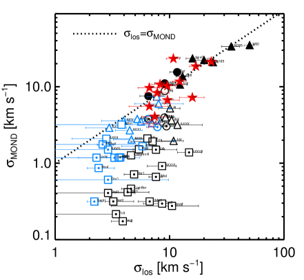
Figure 11: Velocity dispersion of LG dwarfs compared with MOND predictions and taking into account external field effects (Eq. 8). Systems with $g_{\rm in}>g_{\rm ex}$ are shown with filled symbols; systems with $g_{\rm ex}>g_{\rm in}$ are shown with open symbols. Those in the ‘EFE-dominated’ regime ($g_{\rm ex}/g_{\rm in}>5$) are highlighted with a dot. Note that MOND clearly fails to account for the observed velocity dispersions of many LG dwarfs, especially those at the extremely faint end.

5 Summary and Conclusions

The low velocity dispersions of dwarf galaxies have long been difficult to reconcile with the $\Lambda$CDM standard model of structure formation. This is because dwarfs in $\Lambda$CDM are expected to form in haloes above a certain minimum circular velocity of order $20$-$30\,{\rm km}\,\,{\rm s}^{-1}$, which is at odds with the very low velocity dispersions, $\sigma_{\rm los}\sim 3$–$5\,{\rm km}\,\,{\rm s}^{-1}$, of a number of Local Group satellites.

Previously proposed solutions include the possibility that baryons may have reduced the expected dark matter content of a dwarf by carving a constant density ‘core’ in the dark mass profile (Di Cintio et al., 2014; Oñorbe et al., 2015), or, alternatively, that the stellar component of dwarfs samples only the very inner, rising part of the CDM circular velocity curve (Benson et al., 2002; Stoehr et al., 2002). The first possibility has been hinted at by recent simulation work, but it is unlikely to apply in the regime of extremely dark matter-dominated ultra-faint dwarfs, where there are simply not enough baryons to modify the dark matter profile.

The second possibility has been contradicted by the discovery of ‘cold faint giants’; i.e., dwarfs that are exceptional because of their low luminosity, large size and cold kinematics. Examples include Cra 2 and And XIX, dwarfs so large that their stellar kinematics should faithfully sample the maximum circular velocity of the halo, but whose stars are kinematically much colder than expected.

We have examined here the possibility that these issues might be solved by considering the effects of tidal stripping. Our analysis uses the galaxy mass-halo mass relation from the APOSTLE cosmological simulations of the Local Group, as well as guidance from earlier N-body work about the changes induced by tidal stripping on the size, stellar mass, and velocity dispersion of spheroidal galaxies embedded in cuspy CDM haloes. Our main conclusions may be summarized as follows.

• The APOSTLE simulations predict that all faint isolated dwarfs (i.e., $M_{\rm str}<10^{7}\,M_{\odot}$) should inhabit haloes that span a fairly narrow range of virial masses. Together with the self-similar nature of CDM haloes, this implies a strong correlation between dwarf size and characteristic velocity, as larger galaxies should encompass more dark mass. Systems that fail to follow this expected correlation have likely been affected by tidal stripping.

• Prior N-body work on the tidal evolution of dSphs in CDM haloes (PNM08 and E15) allows us to ‘undo’ the effects of tides on the size, mass, and velocity dispersion of a satellite. The change in each of these parameters is linked to the others through ‘tidal tracks’ that may be used to recover the original structural parameters of a satellite’s progenitor. Importantly, these tracks suggest that the stellar half-mass radius of a satellite is the least affected by tides, even for cases of extreme mass loss.

• Satellite progenitors, when constrained to match the APOSTLE $M_{\rm str}$ vs $V_{\rm max}$ relation, follow scaling laws linking the stellar mass, size, and velocity dispersion that are in excellent agreement with those of isolated field galaxies. This provides an attractive explanation for (i) why the [Fe/H]-$\sigma$ relation flattens at low $\sigma$; (ii) why some faint satellites are extremely large (they are the tidal remnants of once more massive, intrinsically large galaxies), and (iii) why satellites and field dwarfs follow a similar dynamical mass-to-light ratio vs luminosity relation, regardless of stripping.

• Tidally stripped satellites are closer than the average to the centre of their host, but even very highly tidally-stripped systems are found as out as $\sim 200$ kpc from the centre. We find no obvious inconsistency between the degree of tidal stripping predicted by our models and the measured spatial distribution of LG satellites.

• Tidal stripping is expected to result in large scatter at the faint, low-acceleration end of the mass discrepancy-acceleration relation (MDAR) that holds for brighter late-type galaxies. Satellites that have lost substantial amounts of dark matter to tides are pushed to accelerations well below the nominal minimum, $a_{\rm min}=10^{-11}{\rm m\,s}^{-2}$, expected for isolated dwarfs in $\Lambda$CDM. The expected scatter is consistent with LG dwarf observations, but inconsistent with the idea that a single MDAR relation holds for all galaxies.

• Finally, the low velocity dispersion population of satellites is plainly inconsistent with the predictions of Modified Newtonian Dynamics: MOND predicts, at the very faint end, much lower velocity dispersions than observed. Resorting to ‘external field effects’ induced by the primaries does not help, and actually makes MOND predictions even more inconsistent with extant data. The velocity dispersions of the faintest galaxies known might prove an insurmountable difficulty for this theory.

Although appealing as a scenario, our proposal that tidal stripping might help to reconcile the peculiar properties of a number of satellites with the predictions of $\Lambda$CDM has a number of potential problems that need to be fully addressed in future work and that would also benefit from insight from other cosmological simulations of Local Group environments (see; e.g., Wang et al., 2015; Wetzel et al., 2016). One potentially weak point concerns the relatively high frequency of highly stripped LG satellites required to match the LG dwarfs. Indeed, we find that about $\sim 11$ ($16$) per cent of MW and M31 satellites brighter than $M_{V}=-8$ ($-5.5$) have lost more than $90$ per cent of their original stellar mass. Unfortunately, current APOSTLE simulations do not have adequate numerical resolution to make accurate predictions that may be compared with these data. This is an issue, however, that should be revisited with simulations of higher resolution, as they become available.

A further, related point is that a number of dwarfs are deemed to have undergone rather dramatic transformation because of tides. Cra 2, And XIX, And XXI, And XXV, and Bootes 1, for example, would all need to have shed roughly $99$ per cent of their original mass for their progenitors to be consistent with APOSTLE dwarfs, yet there is little evidence in the galaxies themselves or in their surroundings for this rather extreme mass loss. Simulations, however, make some fairly robust predictions for these heavily-stripped satellites that may be constrasted with observation. Because they have been so heavily shaken by tides, we expect them their remnants to be round and their surface brightness profiles to have large King concentration values. In addition, because they have been stripped of their surrounding halos, their maximum circular velocities must be very similar to that inferred within their stellar half-mass radius, a prediction that may in principle be tested with accurate dynamical modeling of kinematic data.

Of course, identifying and quantifying debris from such events in the halo of the Milky Way that may be traced back to these satellites would also be an important step towards turning our proposal from informed conjecture into a compelling picture. We anticipate, however, that this task will be rather difficult, given the extremely low surface brightness expected for the stream (fainter than the bound remnants, some of which are already at the limit of detectability). Another possibility would be to look for loosely bound stars in the immediate vicinity of the tidally affected dwarf, which would flatten the satellite surface density profile outside a characteristic radius (Peñarrubia et al., 2009). Detecting such stars would also be extremely challenging, since simulations indicate that their surface brightness, at apocentre, might be up to $\sim 10$ magnitudes fainter than the central surface density of the satellite (see, e.g., Tomozeiu et al., 2016).

Proper motions of individual stars would be of immense help. These could be used to estimate pericentric distances and orbital times that may be used to check the consistency of our model with more detailed modelling of each individual system suspected to be a ‘tidal remnant’. We very much look forward to such data in order to inform our analysis further in future work.

6 Acknowledgements

We acknowledge useful discussions with Alan McConnachie and Joop Schaye. We are thankful to Marla Geha, Erik Tollerud, and Ryan Leaman for sharing data with us. The research was supported in part by the Science and Technology Facilities Council Consolidated Grant (ST/P000541/1), and the European Research Council under the European Union Seventh Framework Programme (FP7/2007-2013)/ERC Grant agreement 278594-GasAroundGalaxies. CSF acknowledges ERC Advanced Grant 267291 COSMIWAY; and JW the 973 program grant 2015CB857005 and NSFC grant No. 11373029, 11390372. This work used the DiRAC Data Centric system at Durham University, operated by the Institute for Computational Cosmology on behalf of the STFC DiRAC HPC Facility (www.dirac.ac.uk), and also resources provided by WestGrid (www.westgrid.ca) and Compute Canada (www.computecanada.ca). The DiRAC system was funded by BIS National E-infrastructure capital grant ST/K00042X/1, STFC capital grants ST/H008519/1 and ST/K00087X/1, STFC DiRAC Operations grant ST/K003267/1 and Durham University. DiRAC is part of the National E-Infrastructure. This research has made use of NASA’s Astrophysics Data System.

Appendix A Parameters for dwarf galaxies in the Local Group

Table of the observed parameters of dwarf galaxies in the Local Group, adopted in this work, along with tables containing derived parameters.

References: Most parameters are adopted from the updated (October 2015) version of the tables from McConnachie (2012). We also use parameters from other references, including the following: 1: McConnachie (2012), 2: Torrealba et al. (2016), 3: Caldwell et al. (2017), 4: Koposov et al. (2015), 5:Walker et al. (2016), 6: Martin et al. (2016a), 7: Kirby et al. (2015), 8: Kirby et al. (2017b), 9: Tollerud et al. (2012), 10: Ho et al. (2012), 11: Collins et al. (2013), 12: Tollerud et al. (2013), 13: Collins et al. (2010), 14: Martin et al. (2016b), 15: Kirby et al. (2014), 16: Hunter & Elmegreen (2006), 17: Leaman et al. (2012), 18: Bellazzini et al. (2011), 19: Kirby et al. (2017a), 20: McConnachie & Irwin (2006), 21: Crnojević et al. (2016), 22: Li et al. (2017).

Table 2: Observed parameters of dwarf galaxies in the Local Group

Gal. Name	$m_{V}$	$(m-M)_{0}$	$R_{\rm eff}$	$\sigma_{\rm los}$	$M_{\rm str}/L_{V}$	[Fe/H]	$D_{\rm host}$	references
			(arcmin)	($\,{\rm km}\,\,{\rm s}^{-1}$)		(dex)	(kpc)
MW satellites
For	$7.4^{+0.3}_{-0.3}$	$20.84^{+0.18}_{-0.18}$	$16.6^{+1.2}_{-1.2}$	$11.7^{+0.9}_{-0.9}$	$1.2$	$-0.90\pm 0.01$	$149$	1
LeoI	$10.0^{+0.3}_{-0.3}$	$22.02^{+0.13}_{-0.13}$	$3.4^{+0.3}_{-0.3}$	$9.2^{+1.4}_{-1.4}$	$0.9$	$-1.40\pm 0.01$	$256$	1
Scl	$8.6^{+0.5}_{-0.5}$	$19.67^{+0.14}_{-0.14}$	$11.3^{+1.6}_{-1.6}$	$9.2^{+1.1}_{-1.1}$	$1.7$	$-1.60\pm 0.01$	$85$	1
LeoII	$12.0^{+0.3}_{-0.3}$	$21.84^{+0.13}_{-0.13}$	$2.6^{+0.6}_{-0.6}$	$6.6^{+0.7}_{-0.7}$	$1.6$	$-1.60\pm 0.01$	$235$	1
SexI	$10.4^{+0.5}_{-0.5}$	$19.67^{+0.10}_{-0.10}$	$27.8^{+1.2}_{-1.2}$	$7.9^{+1.3}_{-1.3}$	$1.6$	$-1.90\pm 0.01$	$88$	1
Car	$11.0^{+0.5}_{-0.5}$	$20.11^{+0.13}_{-0.13}$	$8.2^{+1.2}_{-1.2}$	$6.6^{+1.2}_{-1.2}$	$1.0$	$-1.70\pm 0.01$	$106$	1
Dra	$10.6^{+0.2}_{-0.2}$	$19.40^{+0.17}_{-0.17}$	$10.0^{+0.3}_{-0.3}$	$9.1^{+1.2}_{-1.2}$	$1.8$	$-1.90\pm 0.01$	$75$	1
Umi	$10.6^{+0.5}_{-0.5}$	$19.40^{+0.10}_{-0.10}$	$19.9^{+1.9}_{-1.9}$	$9.5^{+1.2}_{-1.2}$	$1.9$	$-2.10\pm 0.01$	$77$	23
CanVenI	$13.1^{+0.2}_{-0.2}$	$21.69^{+0.10}_{-0.10}$	$8.9^{+0.4}_{-0.4}$	$7.6^{+0.4}_{-0.4}$	$1.6$	$-1.90\pm 0.01$	$216$	1
CraII	$12.1^{+0.1}_{-0.1}$	$20.35^{+0.02}_{-0.02}$	$29.2^{+2.4}_{-2.2}$	$2.8^{+0.3}_{-0.3}$	$1.6$	$-1.98\pm 0.10$	$114$	2,3
Her	$14.0^{+0.3}_{-0.3}$	$20.60^{+0.20}_{-0.20}$	$8.6^{+1.8}_{-1.1}$	$3.7^{+0.9}_{-0.9}$	$1.6$	$-2.40\pm 0.04$	$125$	1
BooI	$12.8^{+0.2}_{-0.2}$	$19.11^{+0.08}_{-0.08}$	$12.6^{+1.0}_{-1.0}$	$2.4^{+0.5}_{-0.9}$	$1.6$	$-2.50\pm 0.11$	$63$	1
LeoIV	$15.1^{+0.4}_{-0.4}$	$20.94^{+0.09}_{-0.09}$	$4.6^{+0.8}_{-0.8}$	$3.3^{+1.7}_{-1.7}$	$1.6$	$-2.50\pm 0.07$	$154$	1
UMaI	$14.4^{+0.3}_{-0.3}$	$19.93^{+0.10}_{-0.10}$	$11.3^{+1.7}_{-1.7}$	$7.6^{+1.0}_{-1.0}$	$1.6$	$-2.10\pm 0.04$	$100$	1
LeoV	$16.0^{+0.4}_{-0.4}$	$21.25^{+0.12}_{-0.12}$	$2.6^{+0.6}_{-0.6}$	$2.3^{+1.6}_{-3.2}$	$1.6$	$-2.00\pm 0.20$	$177$	1
PisII	$16.3^{+0.5}_{-0.5}$	$21.30^{+0.50}_{-0.50}$	$1.1^{+0.1}_{-0.1}$	$5.4^{+2.4}_{-3.6}$	$1.6$	$-2.45\pm 0.07$	$180$	7
CanVeniII	$16.1^{+0.5}_{-0.5}$	$21.02^{+0.06}_{-0.06}$	$1.6^{+0.3}_{-0.3}$	$4.6^{+1.0}_{-1.0}$	$1.6$	$-2.20\pm 0.05$	$159$	1
HydII	$15.8^{+0.3}_{-0.3}$	$20.64^{+0.16}_{-0.16}$	$1.7^{+0.3}_{-0.2}$	$<3.6$	$1.6$	$-2.00\pm 0.08$	$131$	7
UMaII	$13.3^{+0.5}_{-0.5}$	$17.50^{+0.30}_{-0.30}$	$16.0^{+1.0}_{-1.0}$	$6.7^{+1.4}_{-1.4}$	$1.6$	$-2.40\pm 0.06$	$37$	1
ComBer	$14.1^{+0.5}_{-0.5}$	$18.20^{+0.20}_{-0.20}$	$6.0^{+0.6}_{-0.6}$	$4.6^{+0.8}_{-0.8}$	$1.6$	$-2.60\pm 0.05$	$44$	1
Tuc2	$15.0^{+0.1}_{-0.1}$	$18.80^{+0.20}_{-0.20}$	$9.8^{+1.7}_{-1.1}$	$8.6^{+2.7}_{-4.4}$	$1.6$	$-2.23\pm 0.15$	$53$	5
Hor1	$16.1^{+0.1}_{-0.1}$	$19.50^{+0.20}_{-0.20}$	$1.3^{+0.2}_{-0.1}$	$4.9^{+0.9}_{-2.8}$	$1.6$	$-2.76\pm 0.17$	$79$	4
Gru1	$17.0^{+0.3}_{-0.3}$	$20.40^{+0.20}_{-0.20}$	$1.8^{+0.9}_{-0.4}$	$2.9^{+2.1}_{-6.9}$	$1.6$	$-1.42\pm 0.50$	$116$	5
DraII	$14.0^{+0.8}_{-0.8}$	$16.90^{+0.30}_{-0.30}$	$2.7^{+1.0}_{-0.8}$	$2.9^{+2.1}_{-2.1}$	$1.6$	$-2.20$	$25$	6
BooII	$15.4^{+0.9}_{-0.9}$	$18.10^{+0.06}_{-0.06}$	$4.2^{+1.4}_{-1.4}$	$10.5^{+7.4}_{-7.4}$	$1.6$	$-1.70\pm 0.05$	$38$	1
Ret2	$14.7^{+0.1}_{-0.1}$	$17.40^{+0.20}_{-0.20}$	$3.6^{+0.2}_{-0.1}$	$3.2^{+0.5}_{-1.6}$	$1.6$	$-2.46\pm 0.30$	$31$	4
Will1	$15.2^{+0.7}_{-0.7}$	$17.90^{+0.40}_{-0.40}$	$2.3^{+0.4}_{-0.4}$	$4.3^{+1.3}_{-2.3}$	$1.6$	$-2.10$	$42$	1
SegII	$15.2^{+0.3}_{-0.3}$	$17.70^{+0.10}_{-0.10}$	$3.4^{+0.2}_{-0.2}$	$2.2^{+0.3}_{-0.3}$	$1.6$	$-2.20\pm 0.13$	$40$	1
TriII	$15.6^{+0.5}_{-0.5}$	$17.40^{+0.10}_{-0.10}$	$3.9^{+1.1}_{-0.9}$	$<3.4$	$1.6$	$-2.50$	$36$	8
SegI	$15.3^{+0.8}_{-0.8}$	$16.80^{+0.20}_{-0.20}$	$4.4^{+1.2}_{-0.6}$	$3.9^{+0.8}_{-0.8}$	$1.6$	$-2.70\pm 0.40$	$27$	1
M31 satellites
N205	$8.1^{+0.1}_{-0.1}$	$24.58^{+0.07}_{-0.07}$	$2.5^{+0.1}_{-0.1}$	$35.0^{+5.0}_{-5.0}$	$1.4$	$-0.80\pm 0.20$	$41$	1
M32	$8.1^{+0.1}_{-0.1}$	$24.53^{+0.21}_{-0.21}$	$0.5^{+0.1}_{-0.1}$	$50.0^{+0.0}_{-0.0}$	$1.6$	$-0.20$	$22$	1
N185	$9.2^{+0.1}_{-0.1}$	$23.95^{+0.09}_{-0.09}$	$1.5^{+0.0}_{-0.0}$	$24.0^{+1.0}_{-1.0}$	$1.0$	$-1.30\pm 0.10$	$187$	1
N147	$9.5^{+0.1}_{-0.1}$	$24.15^{+0.09}_{-0.09}$	$2.0^{+0.0}_{-0.0}$	$16.0^{+1.0}_{-1.0}$	$1.6$	$-1.10\pm 0.10$	$142$	1
AVII	$11.2^{+0.3}_{-0.3}$	$24.41^{+0.10}_{-0.10}$	$3.5^{+0.1}_{-0.1}$	$13.0^{+1.0}_{-1.0}$	$0.9$	$-1.40\pm 0.30$	$218$	9
AII	$11.5^{+0.2}_{-0.2}$	$24.07^{+0.06}_{-0.06}$	$6.2^{+0.2}_{-0.2}$	$7.8^{+1.1}_{-1.1}$	$1.0$	$-1.30\pm 0.03$	$184$	10,14
AI	$12.5^{+0.1}_{-0.1}$	$24.36^{+0.07}_{-0.07}$	$3.1^{+0.3}_{-0.3}$	$10.2^{+1.9}_{-1.9}$	$1.6$	$-1.40\pm 0.04$	$58$	9,14
AVI	$13.0^{+0.2}_{-0.2}$	$24.47^{+0.07}_{-0.07}$	$2.3^{+0.2}_{-0.2}$	$12.4^{+1.5}_{-1.3}$	$1.6$	$-1.50\pm 0.10$	$268$	11
AXXIII	$14.2^{+0.5}_{-0.5}$	$24.43^{+0.13}_{-0.13}$	$4.6^{+0.2}_{-0.2}$	$7.1^{+1.0}_{-1.0}$	$1.6$	$-2.20\pm 0.30$	$126$	11,14
AIII	$14.2^{+0.3}_{-0.3}$	$24.37^{+0.07}_{-0.07}$	$2.2^{+0.2}_{-0.2}$	$9.3^{+1.4}_{-1.4}$	$1.8$	$-1.70\pm 0.04$	$75$	9,14
LGS3	$14.3^{+0.1}_{-0.1}$	$24.43^{+0.07}_{-0.07}$	$2.1^{+0.2}_{-0.2}$	$7.9^{+5.3}_{-2.9}$	$1.0$	$-2.10\pm 0.22$	$268$	1
AXXI	$14.8^{+0.6}_{-0.6}$	$24.59^{+0.06}_{-0.07}$	$3.5^{+0.3}_{-0.3}$	$4.5^{+1.2}_{-1.0}$	$1.6$	$-1.80\pm 0.10$	$133$	11,14
AXXV	$14.8^{+0.5}_{-0.5}$	$24.55^{+0.12}_{-0.12}$	$3.0^{+0.2}_{-0.2}$	$3.0^{+1.2}_{-1.1}$	$1.6$	$-1.90\pm 0.10$	$88$	11,14
AV	$14.9^{+0.2}_{-0.2}$	$24.44^{+0.08}_{-0.08}$	$1.4^{+0.2}_{-0.2}$	$10.5^{+1.1}_{-1.1}$	$1.1$	$-2.00\pm 0.10$	$109$	9,14
AXV	$14.6^{+0.3}_{-0.3}$	$23.98^{+0.26}_{-0.12}$	$1.2^{+0.1}_{-0.1}$	$4.0^{+1.4}_{-1.4}$	$1.6$	$-1.80\pm 0.20$	$178$	9,14
AXIX	$15.6^{+0.6}_{-0.6}$	$24.57^{+0.08}_{-0.43}$	$6.2^{+0.1}_{-0.1}$	$4.7^{+1.6}_{-1.4}$	$1.6$	$-1.80\pm 0.30$	$113$	11,14
AXIV	$15.9^{+0.5}_{-0.5}$	$24.50^{+0.06}_{-0.56}$	$1.7^{+0.8}_{-0.8}$	$5.3^{+1.0}_{-1.0}$	$1.6$	$-2.20\pm 0.05$	$161$	9,14
AXXIX	$16.0^{+0.4}_{-0.4}$	$24.32^{+0.22}_{-0.22}$	$1.7^{+0.2}_{-0.2}$	$5.7^{+1.2}_{-1.2}$	$1.6$	$-1.80$	$188$	12
AIX	$16.3^{+1.1}_{-1.1}$	$24.42^{+0.07}_{-0.07}$	$2.5^{+0.1}_{-0.1}$	$10.9^{+2.0}_{-2.0}$	$1.6$	$-2.20\pm 0.20$	$40$	9,14
AXXX	$16.2^{+0.3}_{-0.3}$	$24.17^{+0.10}_{-0.26}$	$1.4^{+0.1}_{-0.2}$	$11.8^{+7.7}_{-4.7}$	$1.6$	$-1.70\pm 0.40$	$147$	11,14
AXXVII	$16.7^{+0.5}_{-0.7}$	$24.59^{+0.12}_{-0.12}$	$1.8^{+0.3}_{-0.3}$	$14.8^{+3.1}_{-4.3}$	$1.6$	$-2.10\pm 0.50$	$73$	11,14
AXVII	$16.6^{+0.3}_{-0.3}$	$24.31^{+0.11}_{-0.08}$	$1.4^{+0.3}_{-0.3}$	$2.9^{+1.9}_{-2.2}$	$1.6$	$-1.70\pm 0.20$	$70$	11,14
AX	$16.7^{+0.3}_{-0.3}$	$24.13^{+0.08}_{-0.13}$	$1.1^{+0.4}_{-0.2}$	$6.4^{+1.4}_{-1.4}$	$1.6$	$-1.90\pm 0.11$	$134$	9,14
AXVI	$16.1^{+0.3}_{-0.3}$	$23.39^{+0.19}_{-0.14}$	$1.0^{+0.1}_{-0.1}$	$3.8^{+2.9}_{-2.9}$	$1.6$	$-2.10\pm 0.20$	$323$	9,14
AXII	$17.7^{+0.5}_{-0.5}$	$24.70^{+0.30}_{-0.30}$	$1.1^{+0.2}_{-0.2}$	$2.6^{+2.6}_{-5.1}$	$1.6$	$-2.20\pm 0.20$	$178$	13,14
AXIII	$17.8^{+0.4}_{-0.4}$	$24.62^{+0.05}_{-0.05}$	$0.8^{+0.4}_{-0.3}$	$5.8^{+2.0}_{-2.0}$	$1.6$	$-1.70\pm 0.30$	$132$	9,14
AXXII	$18.0^{+0.4}_{-0.4}$	$24.82^{+0.07}_{-0.07}$	$0.9^{+0.3}_{-0.2}$	$2.8^{+1.4}_{-1.9}$	$1.6$	$-1.80\pm 0.60$	$273$	11,14
AXX	$18.0^{+0.4}_{-0.4}$	$24.35^{+0.12}_{-0.12}$	$0.4^{+0.2}_{-0.1}$	$7.1^{+2.5}_{-3.9}$	$1.6$	$-2.20\pm 0.40$	$129$	11,14
AXI	$18.0^{+0.4}_{-0.4}$	$24.33^{+0.05}_{-0.05}$	$0.6^{+0.2}_{-0.2}$	$7.6^{+2.8}_{-4.0}$	$1.6$	$-1.80\pm 0.10$	$110$	11,14
AXXVI	$18.5^{+0.7}_{-0.5}$	$24.41^{+0.12}_{-0.12}$	$1.0^{+0.6}_{-0.5}$	$8.6^{+2.2}_{-2.8}$	$1.6$	$-1.80\pm 0.50$	$102$	11,14
LG field dwarfs
N6822	$8.1^{+0.2}_{-0.2}$	$23.31^{+0.08}_{-0.08}$	$3.6^{+0.2}_{-0.2}$	$23.2^{+1.2}_{-1.2}$	$0.8$	$-1.00\pm 0.50$	$451$	15,16
IC1613	$9.2^{+0.1}_{-0.1}$	$24.39^{+0.12}_{-0.12}$	$4.7^{+0.4}_{-0.4}$	$10.8^{+1.0}_{-0.9}$	$1.0$	$-1.60\pm 0.20$	$757$	15,16
WLM	$10.6^{+0.1}_{-0.1}$	$24.85^{+0.08}_{-0.08}$	$5.8^{+0.4}_{-0.3}$	$17.0^{+1.0}_{-1.0}$	$0.9$	$-1.20\pm 0.02$	$932$	17
UGC4879	$13.2^{+0.2}_{-0.2}$	$25.67^{+0.04}_{-0.04}$	$0.40^{+0.04}_{-0.04}$	$9.6^{+1.3}_{-1.2}$	$0.7$	$-1.50\pm 0.06$	$1367$	15,18
Peg	$12.6^{+0.2}_{-0.2}$	$24.82^{+0.07}_{-0.07}$	$2.6^{+0.2}_{-0.2}$	$12.3^{+1.2}_{-1.1}$	$1.0$	$-1.40\pm 0.20$	$920$	15,16
LeoA	$12.4^{+0.2}_{-0.2}$	$24.51^{+0.12}_{-0.12}$	$1.5^{+0.1}_{-0.1}$	$6.7^{+1.4}_{-1.2}$	$0.5$	$-1.40\pm 0.20$	$801$	19,16
Cet	$13.1^{+0.2}_{-0.2}$	$24.39^{+0.07}_{-0.07}$	$3.2^{+0.1}_{-0.1}$	$8.3^{+1.0}_{-1.0}$	$1.6$	$-1.90\pm 0.10$	$755$	20,16
Aqu	$14.5^{+0.1}_{-0.1}$	$25.15^{+0.08}_{-0.08}$	$1.5^{+0.04}_{-0.04}$	$7.9^{+1.9}_{-1.6}$	$1.0$	$-1.30\pm 0.20$	$1065$	20,16
Tuc	$15.2^{+0.2}_{-0.2}$	$24.74^{+0.12}_{-0.12}$	$1.1^{+0.0}_{-0.0}$	$15.8^{+4.1}_{-3.1}$	$1.6$	$-1.90\pm 0.15$	$882$	1
AXVIII	$16.0^{+0.2}_{-0.2}$	$25.42^{+0.07}_{-0.08}$	$0.9^{+0.1}_{-0.1}$	$9.7^{+2.3}_{-2.3}$	$1.6$	$-1.40\pm 0.30$	$1216$	9
AXXVIII	$15.6^{+0.4}_{-0.9}$	$24.10^{+0.50}_{-0.20}$	$1.1^{+0.2}_{-0.2}$	$6.6^{+2.9}_{-2.1}$	$1.6$	$-2.10\pm 0.30$	$660$	11
LeoT	$15.1^{+0.5}_{-0.5}$	$23.10^{+0.10}_{-0.10}$	$1.0^{+0.1}_{-0.1}$	$7.5^{+1.6}_{-1.6}$	$0.8$	$-2.00\pm 0.05$	$421$	1
EriII	$15.7^{+0.2}_{-0.2}$	$22.80^{+0.10}_{-0.10}$	$2.3^{+0.1}_{-0.1}$	$6.9^{+1.2}_{-0.9}$	$1.6$	$-2.38\pm 0.13$	$381$	21,22

Table 3: Derived parameters for dwarf galaxies in the Local Group

Gal. Name	$M_{\rm str}$	$r_{1/2}$	$V_{1/2}$	log $g_{\rm bar}$	log $g_{\rm tot}$	$\sigma_{\rm iMOND}$	$\sigma_{\rm eMOND}$	log $g_{\rm in}$	log $g_{\rm ex}$
	($10^{5}\,{\rm M}_{\odot}$)	(pc)	($\,{\rm km}\,\,{\rm s}^{-1}$)	(${\,{\rm m}\,{\rm s}^{-2}}$)	(${\,{\rm m}\,{\rm s}^{-2}}$)	($\,{\rm km}\,\,{\rm s}^{-1}$)	($\,{\rm km}\,\,{\rm s}^{-1}$)	(${\,{\rm m}\,{\rm s}^{-2}}$)	(${\,{\rm m}\,{\rm s}^{-2}}$)
MW satellites
For	$245_{-69}^{+96}$	$949_{-100}^{+106}$	$20.2_{-2.8}^{+2.8}$	$-11.7_{-0.1}^{+0.1}$	$-10.9_{-0.1}^{+0.1}$	$11.8$	$20.6$	$-13.8$	$-14.0$
LeoI	$45_{-13}^{+19}$	$334_{-34}^{+36}$	$15.7_{-2.9}^{+3.1}$	$-11.5_{-0.1}^{+0.1}$	$-10.6_{-0.2}^{+0.2}$	$7.9$	$20.5$	$-13.7$	$-14.2$
Scl	$39_{-15}^{+25}$	$376_{-58}^{+58}$	$15.7_{-2.6}^{+2.8}$	$-11.7_{-0.2}^{+0.2}$	$-10.7_{-0.2}^{+0.2}$	$7.4$	$9.8$	$-13.8$	$-13.7$
LeoII	$12_{-3}^{+4.4}$	$235_{-56}^{+56}$	$11.3_{-1.8}^{+1.8}$	$-11.8_{-0.2}^{+0.3}$	$-10.8_{-0.2}^{+0.2}$	$5.5$	$11.4$	$-13.9$	$-14.2$
SexI	$7.0_{-3}^{+4.3}$	$926_{-56}^{+61}$	$13.6_{-2.7}^{+2.8}$	$-13.2_{-0.2}^{+0.2}$	$-11.2_{-0.2}^{+0.2}$	$4.8$	$2.7$	$-14.6$	$-13.7$
Car	$3.8_{-1.4}^{+2.3}$	$334_{-51}^{+54}$	$11.2_{-2.4}^{+2.6}$	$-12.6_{-0.2}^{+0.2}$	$-10.9_{-0.2}^{+0.2}$	$4.2$	$3.6$	$-14.3$	$-13.8$
Dra	$5.1_{-1.2}^{+1.5}$	$294_{-24}^{+25}$	$15.6_{-2.8}^{+2.8}$	$-12.4_{-0.1}^{+0.1}$	$-10.6_{-0.2}^{+0.2}$	$4.5$	$3.8$	$-14.2$	$-13.7$
Umi	$5.3_{-2.0}^{+3.3}$	$584_{-62}^{+63}$	$16.3_{-2.8}^{+2.9}$	$-13.0_{-0.2}^{+0.2}$	$-10.8_{-0.2}^{+0.1}$	$4.5$	$2.8$	$-14.5$	$-13.7$
CanVenI	$3.7_{-0.8}^{+0.9}$	$751_{-47}^{+49}$	$13.1_{-1.7}^{+1.7}$	$-13.3_{-0.1}^{+0.1}$	$-11.1_{-0.1}^{+0.1}$	$4.1$	$3.4$	$-14.7$	$-14.1$
CraII	$2.6_{-0.3}^{+0.4}$	$1332_{-100}^{+109}$	$4.8_{-0.8}^{+0.8}$	$-14.0_{-0.1}^{+0.1}$	$-12.3_{-0.1}^{+0.1}$	$3.8$	$1.6$	$-15.0$	$-13.9$
Her	$0.60_{-0.18}^{+0.23}$	$443_{-71}^{+99}$	$6.3_{-1.7}^{+1.8}$	$-13.7_{-0.2}^{+0.2}$	$-11.5_{-0.3}^{+0.2}$	$2.3$	$1.1$	$-14.9$	$-13.9$
BooI	$0.46_{-0.09}^{+0.11}$	$325_{-28}^{+29}$	$4.0_{-1.5}^{+1.1}$	$-13.5_{-0.1}^{+0.1}$	$-11.8_{-0.4}^{+0.2}$	$2.2$	$0.8$	$-14.8$	$-13.6$
LeoIV	$0.29_{-0.09}^{+0.14}$	$275_{-49}^{+50}$	$5.7_{-2.7}^{+3.1}$	$-13.6_{-0.2}^{+0.2}$	$-11.4_{-0.6}^{+0.4}$	$2.0$	$1.1$	$-14.9$	$-14.0$
UMaI	$0.22_{-0.06}^{+0.08}$	$423_{-65}^{+68}$	$13.1_{-2.3}^{+2.4}$	$-14.1_{-0.2}^{+0.2}$	$-10.9_{-0.2}^{+0.2}$	$1.8$	$0.6$	$-15.1$	$-13.8$
LeoV	$0.17_{-0.06}^{+0.08}$	$179_{-42}^{+43}$	$4.7_{-2.8}^{+2.6}$	$-13.4_{-0.2}^{+0.3}$	$-11.4_{-0.8}^{+0.4}$	$1.7$	$1.1$	$-14.8$	$-14.1$
PisII	$0.14_{-0.07}^{+0.13}$	$77_{-17}^{+22}$	$9.4_{-5.1}^{+4.4}$	$-12.8_{-0.2}^{+0.2}$	$-10.4_{-0.7}^{+0.4}$	$1.6$	$1.5$	$-14.5$	$-14.1$
CanVeniI	$0.13_{-0.05}^{+0.08}$	$99_{-18}^{+19}$	$7.8_{-1.9}^{+2.1}$	$-13.0_{-0.3}^{+0.3}$	$-10.7_{-0.3}^{+0.2}$	$1.6$	$1.2$	$-14.6$	$-14.0$
HydII	$0.13_{-0.03}^{+0.05}$	$89_{-13}^{+16}$	$7.1_{-1.2}^{+5.5}$	$-13.0_{-0.2}^{+0.2}$	$-10.7_{-0.2}^{+0.5}$	$1.6$	$1.1$	$-14.6$	$-13.9$
UMaII	$0.065_{-0.03}^{+0.05}$	$196_{-27}^{+31}$	$11.4_{-2.5}^{+3.0}$	$-13.9_{-0.2}^{+0.2}$	$-10.7_{-0.2}^{+0.2}$	$1.3$	$0.3$	$-15.0$	$-13.4$
ComBer	$0.060_{-0.02}^{+0.04}$	$101_{-13}^{+14}$	$7.9_{-1.6}^{+1.7}$	$-13.4_{-0.2}^{+0.2}$	$-10.7_{-0.2}^{+0.2}$	$1.3$	$0.4$	$-14.8$	$-13.5$
Tuc2	$0.045_{-0.01}^{+0.012}$	$222_{-33}^{+41}$	$14.4_{-6.6}^{+5.3}$	$-14.2_{-0.1}^{+0.1}$	$-10.5_{-0.5}^{+0.3}$	$1.2$	$0.3$	$-15.2$	$-13.5$
Hor1	$0.031_{-0.006}^{+0.008}$	$41_{-6}^{+7}$	$8.0_{-3.9}^{+2.2}$	$-12.9_{-0.1}^{+0.1}$	$-10.3_{-0.6}^{+0.2}$	$1.1$	$0.7$	$-14.5$	$-13.7$
Gru1	$0.031_{-0.009}^{+0.013}$	$84_{-21}^{+38}$	$6.5_{-3.3}^{+3.0}$	$-13.5_{-0.3}^{+0.3}$	$-10.8_{-0.6}^{+0.4}$	$1.1$	$0.6$	$-14.8$	$-13.9$
DraII	$0.020_{-0.011}^{+0.025}$	$25_{-8}^{+10}$	$5.3_{-3.0}^{+3.5}$	$-12.7_{-0.4}^{+0.4}$	$-10.4_{-0.7}^{+0.5}$	$1.0$	$0.4$	$-14.4$	$-13.2$
BooII	$0.016_{-0.009}^{+0.021}$	$68_{-22}^{+23}$	$19.3_{-10.8}^{+12.7}$	$-13.6_{-0.5}^{+0.5}$	$-9.7_{-0.7}^{+0.5}$	$1.0$	$0.3$	$-14.9$	$-13.4$
Ret2	$0.016_{-0.003}^{+0.004}$	$43_{-4}^{+5}$	$5.3_{-2.4}^{+1.4}$	$-13.2_{-0.1}^{+0.1}$	$-10.7_{-0.5}^{+0.2}$	$1.0$	$0.3$	$-14.7$	$-13.3$
Will1	$0.016_{-0.008}^{+0.018}$	$33_{-8}^{+9}$	$7.1_{-3.3}^{+2.7}$	$-13.0_{-0.3}^{+0.3}$	$-10.3_{-0.6}^{+0.3}$	$1.0$	$0.4$	$-14.6$	$-13.4$
SegII	$0.014_{-0.004}^{+0.005}$	$46_{-3}^{+3}$	$3.8_{-0.6}^{+0.7}$	$-13.3_{-0.1}^{+0.1}$	$-11.0_{-0.2}^{+0.1}$	$0.9$	$0.3$	$-14.8$	$-13.4$
TriII	$0.0071_{-0.0027}^{+0.0045}$	$46_{-11}^{+12}$	$6.6_{-1.1}^{+5.1}$	$-13.6_{-0.3}^{+0.3}$	$-10.5_{-0.2}^{+0.5}$	$0.8$	$0.2$	$-14.9$	$-13.4$
SegI	$0.0054_{-0.0029}^{+0.0063}$	$40_{-7}^{+11}$	$6.6_{-1.5}^{+1.7}$	$-13.6_{-0.4}^{+0.4}$	$-10.5_{-0.2}^{+0.2}$	$0.7$	$0.2$	$-14.9$	$-13.2$
M31 satellites
N205	$4650_{-650}^{+760}$	$786_{-40}^{+41}$	$59.9_{-10.5}^{+11.0}$	$-10.3_{-0.1}^{+0.1}$	$-9.8_{-0.2}^{+0.1}$	$24.6$	$50.1$	$-13.1$	$-13.4$
M32	$4760_{-1010}^{+1260}$	$146_{-20}^{+22}$	$86.7_{-9.1}^{+8.3}$	$-8.8_{-0.1}^{+0.1}$	$-8.8_{-0.1}^{+0.1}$	$24.8$	$86.5$	$-12.4$	$-13.1$
N185	$680_{-100}^{+118}$	$358_{-14}^{+16}$	$41.5_{-4.6}^{+4.3}$	$-10.4_{-0.1}^{+0.1}$	$-9.8_{-0.1}^{+0.1}$	$15.2$	$59.9$	$-13.2$	$-14.0$
N147	$990_{-150}^{+164}$	$532_{-21}^{+22}$	$27.5_{-3.3}^{+3.3}$	$-10.6_{-0.1}^{+0.1}$	$-10.3_{-0.1}^{+0.1}$	$16.7$	$51.8$	$-13.3$	$-13.9$
AVII	$150_{-39}^{+52}$	$1034_{-54}^{+58}$	$22.5_{-2.8}^{+2.8}$	$-12.0_{-0.1}^{+0.1}$	$-10.8_{-0.1}^{+0.1}$	$10.4$	$17.8$	$-14.0$	$-14.1$
AII	$40._{-8}^{+9}$	$1340_{-44}^{+45}$	$13.4_{-2.3}^{+2.4}$	$-12.8_{-0.1}^{+0.1}$	$-11.4_{-0.2}^{+0.1}$	$7.5$	$7.4$	$-14.4$	$-14.0$
AI	$44._{-9}^{+10}$	$1125_{-46}^{+47}$	$17.5_{-3.6}^{+3.9}$	$-12.6_{-0.1}^{+0.1}$	$-11.1_{-0.2}^{+0.2}$	$7.7$	$4.8$	$-14.3$	$-13.5$
AVI	$50._{-10}^{+12}$	$698_{-64}^{+64}$	$21.3_{-3.0}^{+3.3}$	$-12.1_{-0.1}^{+0.1}$	$-10.7_{-0.1}^{+0.1}$	$7.9$	$13.9$	$-14.1$	$-14.2$
AXXIII	$11._{-2}^{+3}$	$1608_{-145}^{+155}$	$12.1_{-2.0}^{+2.2}$	$-13.5_{-0.1}^{+0.1}$	$-11.5_{-0.2}^{+0.1}$	$5.4$	$2.9$	$-14.8$	$-13.9$
AIII	$10._{-2}^{+3}$	$581_{-61}^{+62}$	$15.9_{-2.8}^{+3.0}$	$-12.7_{-0.1}^{+0.1}$	$-10.8_{-0.2}^{+0.2}$	$5.3$	$3.7$	$-14.3$	$-13.6$
LGS3	$9.6_{-1}^{+1.6}$	$625_{-61}^{+64}$	$13.9_{-5.3}^{+8.9}$	$-12.8_{-0.1}^{+0.1}$	$-11.0_{-0.4}^{+0.4}$	$5.3$	$6.5$	$-14.4$	$-14.2$
AXXI	$5.5_{-1.4}^{+1.9}$	$1324_{-142}^{+247}$	$7.8_{-2.0}^{+2.2}$	$-13.7_{-0.2}^{+0.2}$	$-11.8_{-0.3}^{+0.2}$	$4.6$	$2.4$	$-14.8$	$-13.9$
AXXV	$6.3_{-1.6}^{+1.8}$	$864_{-88}^{+125}$	$5.1_{-1.9}^{+2.1}$	$-13.2_{-0.2}^{+0.1}$	$-12.0_{-0.4}^{+0.3}$	$4.7$	$2.6$	$-14.6$	$-13.7$
AV	$5.1_{-1.0}^{+1.3}$	$484_{-38}^{+58}$	$18.0_{-2.6}^{+2.7}$	$-12.8_{-0.1}^{+0.1}$	$-10.7_{-0.1}^{+0.1}$	$4.5$	$3.4$	$-14.4$	$-13.8$
AXV	$2.1_{-0.6}^{+0.8}$	$320_{-32}^{+43}$	$6.8_{-2.4}^{+2.6}$	$-12.9_{-0.1}^{+0.1}$	$-11.3_{-0.4}^{+0.3}$	$3.6$	$3.4$	$-14.4$	$-14.0$
AXIX	$12._{-4}^{+5}$	$4374_{-842}^{+1069}$	$8.0_{-2.5}^{+3.0}$	$-14.4_{-0.2}^{+0.2}$	$-12.3_{-0.3}^{+0.3}$	$5.6$	$1.8$	$-15.2$	$-13.8$
AXIV	$3.3_{-1.2}^{+1.5}$	$431_{-91}^{+77}$	$9.0_{-1.9}^{+2.0}$	$-12.9_{-0.2}^{+0.2}$	$-11.2_{-0.2}^{+0.2}$	$4.0$	$3.6$	$-14.4$	$-14.0$
AXXIX	$2.7_{-0.9}^{+1.5}$	$481_{-73}^{+78}$	$9.7_{-2.2}^{+2.3}$	$-13.1_{-0.2}^{+0.2}$	$-11.2_{-0.2}^{+0.2}$	$3.8$	$3.3$	$-14.5$	$-14.0$
AIX	$4.3_{-1.1}^{+1.5}$	$596_{-64}^{+90}$	$18.8_{-4.0}^{+4.1}$	$-13.1_{-0.2}^{+0.2}$	$-10.7_{-0.2}^{+0.2}$	$4.3$	$1.7$	$-14.5$	$-13.4$
AXXX	$2.2_{-0.6}^{+0.7}$	$385_{-59}^{+62}$	$20.3_{-8.2}^{+13.2}$	$-13.0_{-0.2}^{+0.2}$	$-10.5_{-0.5}^{+0.4}$	$3.6$	$2.9$	$-14.5$	$-13.9$
AXXVII	$2.0_{-0.8}^{+1.8}$	$580_{-101}^{+102}$	$24.7_{-7.4}^{+6.9}$	$-13.4_{-0.3}^{+0.3}$	$-10.5_{-0.3}^{+0.2}$	$3.1$	$1.3$	$-14.8$	$-13.6$
AXVII	$1.7_{-0.4}^{+0.6}$	q$398_{-85}^{+87}$	$5.3_{-3.1}^{+3.2}$	$-13.1_{-0.2}^{+0.2}$	$-11.6_{-0.8}^{+0.4}$	$3.0$	$1.4$	$-14.7$	$-13.6$
AX	$1.3_{-0.3}^{+0.5}$	$287_{-56}^{+102}$	$10.9_{-2.6}^{+2.9}$	$-13.0_{-0.3}^{+0.2}$	$-10.9_{-0.3}^{+0.2}$	$2.8$	$2.0$	$-14.6$	$-13.9$
AXVI	$1.1_{-0.3}^{+0.5}$	$185_{-22}^{+25}$	$7.0_{-4.1}^{+4.8}$	$-12.6_{-0.2}^{+0.2}$	$-11.1_{-0.8}^{+0.5}$	$2.7$	$3.5$	$-14.4$	$-14.3$
AXII	$0.85_{-0.35}^{+0.62}$	$369_{-78}^{+92}$	$6.1_{-3.6}^{+3.9}$	$-13.4_{-0.3}^{+0.3}$	$-11.5_{-0.8}^{+0.4}$	$2.6$	$1.6$	$-14.8$	$-14.0$
AXIII	$0.73_{-0.23}^{+0.33}$	$263_{-97}^{+128}$	$9.9_{-3.5}^{+3.8}$	$-13.1_{-0.4}^{+0.4}$	$-10.9_{-0.4}^{+0.3}$	$2.5$	$1.5$	$-14.6$	$-13.9$
AXXII	$0.73_{-0.23}^{+0.33}$	$323_{-74}^{+105}$	$4.9_{-2.7}^{+2.5}$	$-13.3_{-0.3}^{+0.3}$	$-11.6_{-0.7}^{+0.4}$	$2.5$	$2.0$	$-14.7$	$-14.2$
AXX	$0.48_{-0.16}^{+0.22}$	$116_{-31}^{+57}$	$12.1_{-5.8}^{+4.7}$	$-12.6_{-0.4}^{+0.3}$	$-10.4_{-0.6}^{+0.3}$	$2.2$	$1.8$	$-14.4$	$-13.9$
AXI	$0.46_{-0.15}^{+0.22}$	$171_{-58}^{+57}$	$13.1_{-6.3}^{+5.1}$	$-12.9_{-0.3}^{+0.4}$	$-10.5_{-0.6}^{+0.3}$	$2.2$	$1.4$	$-14.6$	$-13.8$
AXXVI	$0.31_{-0.15}^{+0.20}$	$303_{-141}^{+182}$	$14.4_{-4.7}^{+4.5}$	$-13.6_{-0.5}^{+0.6}$	$-10.7_{-0.4}^{+0.4}$	$2.0$	$0.8$	$-14.9$	$-13.8$
LG field dwarfs
N6822	$830_{-170}^{+200}$	$638_{48}^{50}$	$40.0_{-4.6}^{+4.5}$	$-10.9_{-0.1}^{+0.1}$	$-10.1_{-0.1}^{+0.1}$	$16.0$	$80.4$	$-13.4$	$-14.5$
IC1613	$1020_{-170}^{+190}$	$1383_{135}^{144}$	$18.7_{-2.5}^{+2.5}$	$-11.4_{-0.1}^{+0.1}$	$-11.1_{-0.1}^{+0.1}$	$16.9$	$62.3$	$-13.7$	$-14.5$
WLM	$380_{-55}^{+65}$	$2090_{139}^{149}$	$29.4_{-3.5}^{+3.3}$	$-12.2_{-0.1}^{+0.1}$	$-10.9_{-0.1}^{+0.1}$	$13.2$	$39.4$	$-14.1$	$-14.7$
UGC4879	$58_{-11}^{+13}$	$217_{22}^{21}$	$16.6_{-2.6}^{+2.9}$	$-11.1_{-0.1}^{+0.1}$	$-10.4_{-0.2}^{+0.1}$	$8.2$	$63.7$	$-13.5$	$-14.9$
Peg	$66_{-13}^{+16}$	$928_{64}^{66}$	$21.2_{-2.8}^{+3.0}$	$-12.3_{-0.1}^{+0.1}$	$-10.8_{-0.1}^{+0.1}$	$8.5$	$18.4$	$-14.1$	$-14.4$
LeoA	$30_{-6}^{+8}$	$471_{42}^{45}$	$11.5_{-2.4}^{+2.7}$	$-12.0_{-0.1}^{+0.1}$	$-11.0_{-0.2}^{+0.2}$	$7.0$	$23.6$	$-14.0$	$-14.7$
Cet	$45_{-9}^{+11}$	$936_{41}^{43}$	$14.3_{-2.2}^{+2.3}$	$-12.4_{-0.1}^{+0.1}$	$-11.2_{-0.1}^{+0.1}$	$7.7$	$18.1$	$-14.2$	$-14.6$
Aqu	$16_{-2}^{+3}$	$611_{27}^{28}$	$13.5_{-3.0}^{+3.6}$	$-12.5_{-0.1}^{+0.1}$	$-11.0_{-0.2}^{+0.2}$	$5.9$	$17.3$	$-14.3$	$-14.8$
Tuc	$8.9_{-1.9}^{+2.3}$	$378_{21}^{23}$	$27.4_{-6.2}^{+7.3}$	$-12.4_{-0.1}^{+0.1}$	$-10.2_{-0.2}^{+0.2}$	$5.2$	$15.2$	$-14.2$	$-14.8$
AXVIII	$8.0_{-1.6}^{+1.9}$	$433_{31}^{32}$	$16.6_{-4.1}^{+4.5}$	$-12.5_{-0.1}^{+0.1}$	$-10.7_{-0.2}^{+0.2}$	$5.0$	$9.2$	$-14.2$	$-14.4$
AXXVIII	$4.1_{-1.7}^{+5.2}$	$294_{65}^{82}$	$11.5_{-3.9}^{+5.2}$	$-12.5_{-0.3}^{+0.4}$	$-10.8_{-0.4}^{+0.3}$	$4.2$	$7.2$	$-14.2$	$-14.3$
LeoT	$1.1_{-0.4}^{+0.6}$	$160_{12}^{12}$	$12.8_{-3.0}^{+3.2}$	$-12.5_{-0.2}^{+0.2}$	$-10.5_{-0.2}^{+0.2}$	$3.0$	$5.6$	$-14.2$	$-14.4$
EriII	$0.9_{-0.2}^{+0.2}$	$325_{23}^{23}$	$11.9_{-2.0}^{+2.3}$	$-13.2_{-0.1}^{+0.1}$	$-10.8_{-0.2}^{+0.2}$	$2.9$	$3.5$	$-14.6$	$-14.4$

Table 4: Derived parameters for progenitors of MW and M31 satellites

Progenitor of	$M_{\rm str}$	$3Dr_{1/2}$	$V_{1/2}$	$\mu_{\rm L}$
	($10^{5}\,{\rm M}_{\odot}$)	(pc)	($\,{\rm km}\,\,{\rm s}^{-1}$)
MW satellites
For	300.	864	25.8	0.81
LeoI	49.4	334	15.7	1.00
Scl	39.1	371	16.2	0.99
LeoII	12.4	225	12.4	0.95
SexI	11.5	813	20.8	0.60
Car	4.4	307	13.8	0.85
Dra	5.1	294	15.6	1.00
Umi	5.6	563	17.7	0.95
CanVenI	5.4	665	18.9	0.68
CraII	264	1819	18.1	0.01
Her	4.9	426	15.9	0.12
BooI	46.3	443	15.7	0.01
LeoIV	1.28	250	12.2	0.23
UMaI	0.23	411	14.1	0.96
LeoV	2.25	183	10.8	0.08
PisII	0.137	77	9.4	1.00
CanVeniI	0.127	99	8.0	1.00
HydII	0.127	84	7.0	0.92
UMaII	0.065	196	11.6	1.00
ComBer	0.060	101	8.0	1.00
Tuc2	0.045	219	14.9	1.00
Hor1	0.031	40	8.5	0.99
Gru1	0.039	74	6.5	0.79
DraII	0.020	25	5.0	1.00
BooII	0.016	67	18.2	1.00
Ret2	0.016	42	5.6	0.99
Will1	0.016	33	7.4	0.98
SegII	0.017	41	4.9	0.81
TriII	0.007	45	5.9	0.99
SegI	0.005	39	6.8	0.99
M31 satellites
N205	4650	786	59.9	1.00
M32	5070	146	86.7	1.00
N185	676	358	41.5	1.00
N147	988	532	27.5	1.00
AVII	161	977	25.7	0.92
AII	145	1203	27.3	0.27
AI	60.0	1004	24.3	0.72
AVI	52.8	698	21.3	1.00
AXXIII	64.2	1495	27.5	0.18
AIII	11.1	551	18.0	0.93
LGS3	12.2	565	18.2	0.79
AXXI	593	1808	29.3	0.01
AXXV	681	1180	19.4	0.01
AV	5.12	484	18.0	1.00
AXV	7.42	285	13.6	0.30
AXIX	1336	5975	30.4	0.01
AXIV	7.28	377	15.3	0.49
AXXIX	5.35	421	15.7	0.54
AIX	4.59	596	18.8	1.00
AXXX	2.34	385	20.3	1.00
AXXVII	1.96	578	25.6	1.03
AXVII	168	539	19.0	0.01
AX	1.40	270	12.7	0.90
AXVI	1.91	162	10.2	0.60
AXII	87.4	507	17.0	0.01
AXIII	0.83	242	11.9	0.88
AXXII	47.5	411	17.2	0.02
AXX	0.474	115	12.3	1.01
AXI	0.466	170	13.2	0.99
AXXVI	0.316	295	14.9	0.99

References

- Aguirre et al. (2001) Aguirre A., Schaye J., Quataert E., 2001, ApJ, 561, 550
- Angulo et al. (2012) Angulo R. E., Springel V., White S. D. M., Jenkins A., Baugh C. M., Frenk C. S., 2012, MNRAS, 426, 2046
- Arraki et al. (2014) Arraki K. S., Klypin A., More S., Trujillo-Gomez S., 2014, MNRAS, 438, 1466
- Barber et al. (2015) Barber C., Starkenburg E., Navarro J. F., McConnachie A. W., 2015, MNRAS, 447, 1112
- Bellazzini et al. (2011) Bellazzini M., Perina S., Galleti S., Oosterloo T., 2011, A&A, 533, A37
- Benson et al. (2002) Benson A. J., Lacey C. G., Baugh C. M., Cole S., Frenk C. S., 2002, MNRAS, 333, 156
- Benson et al. (2003) Benson A. J., Bower R. G., Frenk C. S., Lacey C. G., Baugh C. M., Cole S., 2003, ApJ, 599, 38
- Bullock & Boylan-Kolchin (2017) Bullock J. S., Boylan-Kolchin M., 2017, ARA&A, 55, 343
- Caldwell et al. (2017) Caldwell N., et al., 2017, ApJ, 839, 20
- Campbell et al. (2016) Campbell D. J. R., et al., 2016, preprint, (arXiv:1603.04443)
- Collins et al. (2010) Collins M. L. M., et al., 2010, MNRAS, 407, 2411
- Collins et al. (2013) Collins M. L. M., et al., 2013, ApJ, 768, 172
- Crain et al. (2015) Crain R. A., et al., 2015, MNRAS, 450, 1937
- Crnojević et al. (2016) Crnojević D., Sand D. J., Zaritsky D., Spekkens K., Willman B., Hargis J. R., 2016, ApJ, 824, L14
- D’Onghia et al. (2009) D’Onghia E., Besla G., Cox T. J., Hernquist L., 2009, Nature, 460, 605
- Davis et al. (1985) Davis M., Efstathiou G., Frenk C. S., White S. D. M., 1985, ApJ, 292, 371
- Del Popolo & Le Delliou (2017) Del Popolo A., Le Delliou M., 2017, Galaxies, 5, 17
- Di Cintio et al. (2014) Di Cintio A., Brook C. B., Macciò A. V., Stinson G. S., Knebe A., Dutton A. A., Wadsley J., 2014, MNRAS, 437, 415
- Errani et al. (2015) Errani R., Peñarrubia J., Tormen G., 2015, MNRAS, 449, L46
- Fan et al. (2006) Fan X., Carilli C. L., Keating B., 2006, ARA&A, 44, 415
- Fattahi et al. (2016) Fattahi A., et al., 2016, MNRAS, 457, 844
- Fitts et al. (2017) Fitts A., et al., 2017, MNRAS, 471, 3547
- Frings et al. (2017) Frings J., Macciò A., Buck T., Penzo C., Dutton A., Blank M., Obreja A., 2017, MNRAS, 472, 3378
- Geha et al. (2010) Geha M., van der Marel R. P., Guhathakurta P., Gilbert K. M., Kalirai J., Kirby E. N., 2010, ApJ, 711, 361
- Gerbal et al. (1992) Gerbal D., Durret F., Lachieze-Rey M., Lima-Neto G., 1992, A&A, 262, 395
- Governato et al. (2012) Governato F., et al., 2012, MNRAS, 422, 1231
- Guo et al. (2010) Guo Q., White S., Li C., Boylan-Kolchin M., 2010, MNRAS, 404, 1111
- Ho et al. (2012) Ho N., et al., 2012, ApJ, 758, 124
- Hopkins (2013) Hopkins P. F., 2013, MNRAS, 428, 2840
- Hunter & Elmegreen (2006) Hunter D. A., Elmegreen B. G., 2006, ApJS, 162, 49
- Ibata et al. (2001) Ibata R., Irwin M., Lewis G. F., Stolte A., 2001, ApJ, 547, L133
- Jenkins (2013) Jenkins A., 2013, MNRAS, 434, 2094
- Jenkins et al. (2001) Jenkins A., Frenk C. S., White S. D. M., Colberg J. M., Cole S., Evrard A. E., Couchman H. M. P., Yoshida N., 2001, MNRAS, 321, 372
- Kazantzidis et al. (2011) Kazantzidis S., Łokas E. L., Callegari S., Mayer L., Moustakas L. A., 2011, ApJ, 726, 98
- Kirby et al. (2014) Kirby E. N., Bullock J. S., Boylan-Kolchin M., Kaplinghat M., Cohen J. G., 2014, MNRAS, 439, 1015
- Kirby et al. (2015) Kirby E. N., Cohen J. G., Simon J. D., Guhathakurta P., 2015, ApJ, 814, L7
- Kirby et al. (2017a) Kirby E. N., Rizzi L., Held E. V., Cohen J. G., Cole A. A., Manning E. M., Skillman E. D., Weisz D. R., 2017a, ApJ, 834, 9
- Kirby et al. (2017b) Kirby E. N., Cohen J. G., Simon J. D., Guhathakurta P., Thygesen A. O., Duggan G. E., 2017b, ApJ, 838, 83
- Knebe et al. (2011) Knebe A., Libeskind N. I., Knollmann S. R., Martinez-Vaquero L. A., Yepes G., Gottlöber S., Hoffman Y., 2011, MNRAS, 412, 529
- Komatsu et al. (2011) Komatsu E., et al., 2011, ApJS, 192, 18
- Koposov et al. (2015) Koposov S. E., et al., 2015, ApJ, 811, 62
- Kravtsov et al. (2004) Kravtsov A. V., Gnedin O. Y., Klypin A. A., 2004, ApJ, 609, 482
- Leaman et al. (2012) Leaman R., et al., 2012, ApJ, 750, 33
- Lelli et al. (2016a) Lelli F., McGaugh S. S., Schombert J. M., 2016a, AJ, 152, 157
- Lelli et al. (2016b) Lelli F., McGaugh S. S., Schombert J. M., Pawlowski M. S., 2016b, ApJ, 827, L19
- Li et al. (2017) Li T. S., et al., 2017, ApJ, 838, 8
- Ludlow et al. (2009) Ludlow A. D., Navarro J. F., Springel V., Jenkins A., Frenk C. S., Helmi A., 2009, ApJ, 692, 931
- Ludlow et al. (2016) Ludlow A. D., Bose S., Angulo R. E., Wang L., Hellwing W. A., Navarro J. F., Cole S., Frenk C. S., 2016, MNRAS, 460, 1214
- Ludlow et al. (2017) Ludlow A. D., et al., 2017, Physical Review Letters, 118, 161103
- Majewski et al. (2003) Majewski S. R., Skrutskie M. F., Weinberg M. D., Ostheimer J. C., 2003, ApJ, 599, 1082
- Martin et al. (2016a) Martin N. F., et al., 2016a, MNRAS, 458, L59
- Martin et al. (2016b) Martin N. F., et al., 2016b, ApJ, 833, 167
- Mashchenko et al. (2006) Mashchenko S., Couchman H. M. P., Wadsley J., 2006, Nature, 442, 539
- Mateo (1998) Mateo M. L., 1998, ARA&A, 36, 435
- Mayer et al. (2001) Mayer L., Governato F., Colpi M., Moore B., Quinn T., Wadsley J., Stadel J., Lake G., 2001, ApJ, 547, L123
- McConnachie (2012) McConnachie A. W., 2012, AJ, 144, 4
- McConnachie & Irwin (2006) McConnachie A. W., Irwin M. J., 2006, MNRAS, 365, 1263
- McConnachie et al. (2009) McConnachie et al. 2009, Nature, 461, 66
- McGaugh (2016) McGaugh S. S., 2016, ApJ, 832, L8
- McGaugh & Milgrom (2013) McGaugh S., Milgrom M., 2013, ApJ, 766, 22
- McGaugh et al. (2016) McGaugh S. S., Lelli F., Schombert J. M., 2016, Physical Review Letters, 117, 201101
- Milgrom (1983) Milgrom M., 1983, ApJ, 270, 371
- Milgrom (2012) Milgrom M., 2012, Physical Review Letters, 109, 251103
- Moster et al. (2017) Moster B. P., Naab T., White S. D. M., 2017, preprint, (arXiv:1705.05373)
- Navarro et al. (1996a) Navarro J. F., Eke V. R., Frenk C. S., 1996a, MNRAS, 283, L72
- Navarro et al. (1996b) Navarro J. F., Frenk C. S., White S. D. M., 1996b, ApJ, 462, 563
- Navarro et al. (1997) Navarro J. F., Frenk C. S., White S. D. M., 1997, ApJ, 490, 493
- Navarro et al. (2016) Navarro J. F., Benítez-Llambay A., Fattahi A., Frenk C. S., Ludlow A. D., Oman K. A., Schaller M., Theuns T., 2016, preprint, (arXiv:1612.06329)
- Niederste-Ostholt et al. (2010) Niederste-Ostholt M., Belokurov V., Evans N. W., Peñarrubia J., 2010, ApJ, 712, 516
- Oñorbe et al. (2015) Oñorbe J., Boylan-Kolchin M., Bullock J. S., Hopkins P. F., Kereš D., Faucher-Giguère C.-A., Quataert E., Murray N., 2015, MNRAS, 454, 2092
- O’Shea et al. (2015) O’Shea B. W., Wise J. H., Xu H., Norman M. L., 2015, ApJ, 807, L12
- Odenkirchen et al. (2001) Odenkirchen M., et al., 2001, ApJ, 548, L165
- Odenkirchen et al. (2003) Odenkirchen M., et al., 2003, AJ, 126, 2385
- Okamoto & Frenk (2009) Okamoto T., Frenk C. S., 2009, MNRAS, 399, L174
- Oman et al. (2015) Oman K. A., et al., 2015, MNRAS, 452, 3650
- Oman et al. (2016) Oman K. A., Navarro J. F., Sales L. V., Fattahi A., Frenk C. S., Sawala T., Schaller M., White S. D. M., 2016, MNRAS, 460, 3610
- Peñarrubia et al. (2008) Peñarrubia J., Navarro J. F., McConnachie A. W., 2008, ApJ, 673, 226
- Peñarrubia et al. (2009) Peñarrubia J., Navarro J. F., McConnachie A. W., Martin N. F., 2009, ApJ, 698, 222
- Pontzen & Governato (2014) Pontzen A., Governato F., 2014, Nature, 506, 171
- Read & Gilmore (2005) Read J. I., Gilmore G., 2005, MNRAS, 356, 107
- Ricotti et al. (2016) Ricotti M., Parry O. H., Gnedin N. Y., 2016, ApJ, 831, 204
- Sales et al. (2007) Sales L. V., Navarro J. F., Abadi M. G., Steinmetz M., 2007, MNRAS, 379, 1475
- Sanders (2003) Sanders R. H., 2003, MNRAS, 342, 901
- Sawala et al. (2016a) Sawala T., et al., 2016a, MNRAS, 456, 85
- Sawala et al. (2016b) Sawala T., et al., 2016b, MNRAS, 457, 1931
- Schaller et al. (2015a) Schaller M., et al., 2015a, MNRAS, 452, 343
- Schaller et al. (2015b) Schaller M., Dalla Vecchia C., Schaye J., Bower R. G., Theuns T., Crain R. A., Furlong M., McCarthy I. G., 2015b, MNRAS, 454, 2277
- Schaye et al. (2015) Schaye J., et al., 2015, MNRAS, 446, 521
- Springel (2005) Springel V., 2005, MNRAS, 364, 1105
- Springel et al. (2001) Springel V., Yoshida N., White S. D. M., 2001, New Astronomy, 6, 79
- Stoehr et al. (2002) Stoehr F., White S. D. M., Tormen G., Springel V., 2002, MNRAS, 335, L84
- Tinker et al. (2008) Tinker J., Kravtsov A. V., Klypin A., Abazajian K., Warren M., Yepes G., Gottlöber S., Holz D. E., 2008, ApJ, 688, 709
- Tollerud et al. (2012) Tollerud E. J., et al., 2012, ApJ, 752, 45
- Tollerud et al. (2013) Tollerud E. J., Geha M. C., Vargas L. C., Bullock J. S., 2013, ApJ, 768, 50
- Tomozeiu et al. (2016) Tomozeiu M., Mayer L., Quinn T., 2016, ApJ, 818, 193
- Torrealba et al. (2016) Torrealba G., Koposov S. E., Belokurov V., Irwin M., 2016, MNRAS, 459, 2370
- Vogelsberger et al. (2014) Vogelsberger M., et al., 2014, MNRAS, 444, 1518
- Walker et al. (2009) Walker M. G., Mateo M., Olszewski E. W., Peñarrubia J., Wyn Evans N., Gilmore G., 2009, ApJ, 704, 1274
- Walker et al. (2016) Walker M. G., et al., 2016, ApJ, 819, 53
- Wang et al. (2015) Wang L., Dutton A. A., Stinson G. S., Macciò A. V., Penzo C., Kang X., Keller B. W., Wadsley J., 2015, MNRAS, 454, 83
- Wetzel et al. (2016) Wetzel A. R., Hopkins P. F., Kim J.-h., Faucher-Giguère C.-A., Kereš D., Quataert E., 2016, ApJ, 827, L23
- White & Frenk (1991) White S. D. M., Frenk C. S., 1991, ApJ, 379, 52
- Wise et al. (2014) Wise J. H., Demchenko V. G., Halicek M. T., Norman M. L., Turk M. J., Abel T., Smith B. D., 2014, MNRAS, 442, 2560
- Wolf et al. (2010) Wolf J., Martinez G. D., Bullock J. S., Kaplinghat M., Geha M., Muñoz R. R., Simon J. D., Avedo F. F., 2010, MNRAS, 406, 1220
- Woo et al. (2008) Woo J., Courteau S., Dekel A., 2008, MNRAS, 390, 1453