Flux Sensitivity Requirements for the Detection of Lyman Continuum Radiation Drop-ins from Star-forming Galaxies Gelow Redshifts of 3

Abstract

Flux estimates for ionizing radiation escaping from star-forming galaxies with characteristic UV luminosities ($L^{*}_{1500(1+z)}$) derived from GALEX and the VIMOS-VLT Deep Survey, are presented as a function of redshift and assumed escape fraction. These estimates offer guidance to the design of instrumentation and observing strategies, be they spectroscopic or photometric, for attempting to detect LyC escaping star-forming galaxies for redshifts $z<3$. Examples are given that relate the integrated escape fraction ($f^{e}_{LyC}$) of ionizing photons, obtained by integrating over the entire extreme UV (EUV) bandpass, to the relative escape fraction ($f^{e}_{900}$) observed just shortward of the ionization edge at 911.8 Å as a function of H I, He I, and He II column densities. Detection of LyC “drop-ins” in the rest-frame EUV will provide enhanced fidelity to determinations of the integrated fraction of ionizing photons $f^{e}_{LyC}$ that escape star-forming galaxies and contribute to the metagalactic ionizing background (MIB).

1 Introduction

It is evident that most of the hydrogen in the universe was reionized during an Epoch of Reionization (EOR) somewhere between 13.4 and 12.7 Gyr ago, corresponding to redshifts 12 $>z>$ 6 (Fan et al., 2006; Bouwens et al., 2015), when primordial gas clouds began to collapse into proto-galaxies to form the first stars and black holes. Whether the overall increase in ionizing radiation that precipitated the EOR was produced by the first stars or black holes is a major unanswered cosmological question.

The total budget for ionizing radiation escaping from these objects remains uncertain (Madau & Haardt, 2015), but its history plays a crucial role in regulating the subsequent emergence and evolution of structure in the universe (c.f. Madau et al., 1999; Ricotti et al., 2002; Benson et al., 2013; Robertson et al., 2015). Lyman continuum (LyC) photons, emitted below the rest frame H I ionization edge at 911.8 Å, escape the highly ionized confines of quasars and active galactic nuclei (AGNs) with relative ease (Bahcall & Sargent, 1967; Smith et al., 1981; Bechtold et al., 1987; Scott et al., 2004), but the potential contribution from the vastly more numerous star-forming galaxies is harder to quantify; this is due to the difficulty of observing this intrinsically weak emission coupled with our poor understanding of the physical conditions that allow ionizing radiation to escape into the intergalactic medium (IGM).

Empirical estimates of the average escape fraction required to sustain an ionized IGM by $z$ = 6, range from 5 $<f^{e}_{LyC}<$ 40% (Bouwens et al., 2015; Finkelstein et al., 2015, and references therein). These estimates depend on the evolution of the steepness of the galaxy luminosity function, the mean production of LyC emission per unit star-formation rate (SFR), and assumptions regarding the ratio of the escape fraction to the ionized hydrogen clumping factor (Madau et al., 1999). The conclusion that the EOR is driven solely by star-forming galaxies rests on these assumptions, and on an extrapolation of the faint-end cutoff of the galaxy luminosity function from -17 $<M_{uv}<$ -13. Moreover, there are no constraints as to how the escape fraction is distributed as a function of galactic mass, luminosity, and environment.

Cosmological hydrodynamical simulations aiming to determine the escape fraction as a function of luminosity and halo mass have produced mixed results (c.f. Gnedin et al., 2008; Razoumov & Sommer-Larsen, 2010; Yajima et al., 2011; Wise et al., 2014; Yajima et al., 2014). In recent work, Sharma et al. (2016) found that the brighter galaxies have higher escape fractions. In contrast, Xu et al. (2016) find that galaxies with smaller halo masses have the highest escape fractions, however, they also found that star formation in low-mass galaxies is easily suppressed as reionization progresses, leaving higher-mass galaxies, which are less susceptible to photo-evaporation, to complete the process.

One of the key projects for the James Webb Space Telescope (JWST) is to search for those sources responsible for reionizing the universe; however, it will likely only be able to do so indirectly. The monotonic increase with redshift in the density of Lyman limit systems (LLS) – those discrete clouds in the IGM having $\log(N_{HI}(cm^{-2}))>$ 17.2 – steadily decreases the probability of directly detecting LyC emission from star-forming galaxies on an unattenuated line of sight (c.f. Madau, 1995; Inoue & Iwata, 2008; Inoue et al., 2014; Worseck et al., 2014; Crighton et al., 2015). At redshifts of $z$ = [3, 4, 5, 6] the mean transmission of the IGM is estimated to be $\approx$ [0.5, 0.3 0.08, 0.01] (Inoue et al., 2014, their Figure 4), albeit with an large variation about the mean. The JWST  short wavelength cutoff is $\approx$ 0.6 $\mu$m, so the LyC region is accessible only for redshifts $z\gtrsim$ 6 where the IGM is essentially completely opaque. Direct measurements of LyC will be a challenge for JWST, to say the least

The far-UV and near-UV bandpasses provide the most direct path to spatially resolved detection of ionizing radiation, and to the characterization of those environments that favor LyC escape. Spatial resolution is an especially important diagnostic, as models indicate that LyC photons escaping from any particular galaxy will exhibit gross variations that depend on the line of sight of a star-forming source with respect to intervening neutral and ionized material in disks, superbubbles, and surrounding circumgalactic streams Dove & Shull (1994); Bland-Hawthorn & Maloney (1999); Dove et al. (2000); Shull et al. (2015).

Recent successes in detecting LyC emission from what are apparently star-forming galaxies (Leitet et al., 2013; Borthakur et al., 2014; Izotov et al., 2016b; Leitherer et al., 2016; Naidu et al., 2016; Shapley et al., 2016) have emboldened the design of instrumentation and observing strategies capable of quantifying, on an industrial scale, the relative contributions of star-forming galaxies, quasars, and AGN to the creation and sustenance of the metagalactic ionizing background (MIB) across cosmic time.

The need for understanding those physical processes that enable $f^{e}_{LyC}$ at low redshift has grown in importance as of late. Recent determinations of the number density of Ly$\alpha$ forest lines found at low redshift by Danforth et al. (2016) appear to require a MIB $\sim$ 5$\times$ larger than theoretical estimates to explain the low density of the lines (Kollmeier et al., 2014); (see Shull et al., 2015; Gaikwad et al., 2017, for contrasting conclusions). These studies are inconclusive as to whether, on average, $f^{e}_{LyC}$ from star-forming galaxies and quasars is considerably higher than the handful of detections to date indicate, thus underlining the importance of quantifying $f^{e}_{LyC}$ at both low and high redshift.

Our main goal is to establish effective area requirements for future observatories that will transform what has previously been described as an impossible task (Fernandez-Soto et al., 2003), into a statistically significant determination of LyC luminosity function evolution across cosmic time envisioned by Deharveng et al. (1997) and Shull et al. (2015), providing a full accounting of the LyC escape budget from star-forming galaxies of all types.

Here we use 1500 Å luminosity functions to guide estimates of the rest frame EUV flux (the LyC) emitted by characteristic galaxies, attenuated by a uniform foreground screen of circumgalactic media (CGM) with representative ratios of H I, He I, and He II column densities. We also include the progressive increase in mean attenuation effected by the increasing H I distribution of IGM column densities as a function of redshift. A general result is that the LyC escape fraction measured in a narrow range just shortward of the ionization edge is a poor representation of the total fraction of ionizing photons that escape.

These calculations were developed to support science and technology flowdown exercises for the Large Ultra-Violet Optical InfraRed (LUVOIR) and Habitable Exoplanet (HabEx) survey mission studies commissioned by NASA in preparation for the Astrophysics Decadal Survey for 2020, and to assess the capability of proposed probe and explorer class missions.

A cosmology of $H_{0}=$ 70 km s^-1 Mpc^-1, $\Omega_{m}=$ 0.3, $\Omega_{\Lambda}=$ 0.7 is assumed.

1.1 Review of Escape Fraction Terminology

The term “escape fraction” is often used loosely and somewhat conflictingly. The literature defines a number of slightly different ratios to describe the escape of ionizing radiation from galactic environments, which for the sake of completeness we review briefly.

A useful observable, termed the relative escape fraction ($f_{rel}$) by Reddy et al. (2016); Shapley et al. (2006), and Steidel et al. (2001), is defined as the ratio of the observed flux in a bandpass just shortward of the Lyman edge ($F^{o}_{900}$) to that observed at some fiducial UV continuum wavelength ($F^{o}_{\lambda}$);

$$f_{rel}=F^{o}_{900}/F^{o}_{\lambda}.$$ (1)

The observed flux is then relatable to the intrinsic flux ($F^{i}_{\lambda}$) by appeal to a stellar population spectral synthesis model, after accounting for the transmission of flux, $T_{\lambda}$, as attenuated by line of sight neutral gas and dust, such that $F^{o}_{\lambda}=T_{\lambda}F^{i}_{\lambda}$. Just over the edge we have $F^{o}_{900}=f^{e}_{900}F^{i}_{900}$, which Reddy et al. (2016) called $f^{e}_{900}$ the absolute escape fraction (in their notation $f(LyC)_{abs}$).

Solving for $f^{e}_{900}$ in terms of the relative escape fraction, the attenuation at the fiducial wavelength and the intrinsic flux ratio,

$$f^{e}_{900}=T_{\lambda}f_{rel}F^{i}_{\lambda}/F^{i}_{900}.$$ (2)

It explicitly includes hydrogen and dust attenuation at the edge. Borthakur et al. (2014) made a further distinction between what they called a relative escape fraction at 912^-, where $T_{\lambda}$ =1, and an absolute escape fraction at 912^- where they corrected for dust using the ratio of the integrated LyC luminosity, with respect to the bolometric luminosity.

Implicit in these definitions is the assumption that the observed flux $F^{o}_{\lambda}$ is averaged over some relatively narrow bandpass. However, $f^{e}_{900}$ does not fully account for all the ionizing photons that escape from the CGM and contribute to the MIB. To do so requires an integration of the attenuated (“observable”) photon number flux ($F^{o}_{\lambda}/E_{\lambda}$; where $\lambda<$ 911.8 Å and $E_{\lambda}$ is the photon energy) over the full extent of the spectral energy distribution (SED) shortward of the Lyman edge. The integrated escape fraction is normalized by the intrinsic SED integrated over the same wavelength interval,

$$f^{e}_{LyC}=\frac{\int_{0}^{912}F^{o}_{\lambda}/E_{\lambda}d\lambda}{\int_{0}^{912}F^{i}_{\lambda}/E_{\lambda}d\lambda}.$$ (3)

In practice, $F^{o}_{\lambda}$ is not observable in its entirety; however, we can estimate it by the integration of a transmission function, multiplied by the intrinsic flux, $T_{\lambda}F^{i}_{\lambda}$, over the wavelength interval shortward of the Lyman edge.

In § 2 we provide estimates of $F^{o}_{(1+z)900}$ in terms of the characteristic apparent ab-magnitude (abmag) $m_{(1+z)900}$, as a function of $f^{e}_{900}$, scaled from compilations of UV luminosity functions taken from the literature for rest frame wavelengths $\approx$ 1500 Å. In § 3 we will give estimates of the integrated fraction of escaping ionizing photons, $f^{e}_{LyC}$, by modeling the optical depth in neutral hydrogen, neutral helium, and once-ionized helium column in the CGM in the foreground of a spectral synthesis model. In § 4 we include the IGM attenuation in estimating the LyC flux of redshifted models scaled to the magnitudes of characteristic galaxies at (1+$z$)1500 Å, and discuss detection requirements and observing strategies.

Table 1: Schechter parameters for UV Luminosity Functions

$z$	$\Delta z$	$\alpha$	$M^{*}_{15}$	$\phi^{*}$	$m^{*}_{(1+z)1500}$
0.1	0 - 0.2	-1.21	-18.05	4.07	20.17
0.3	0.2 - 0.4	-1.19	-18.38	6.15	22.30
0.5	0.4 - 0.6	-1.55	-19.49	1.69	22.37
0.7	0.5 - 0.8	-1.60	-19.84	1.67	22.73
1.0	0.8 - 1.2	-1.63	-20.11	1.14	23.24
2.0	1.75 - 2.25	-1.49	-20.33	2.65	24.43
2.9	2.4 - 3.4	-1.47	-21.08	1.62	24.38

2 Far-UV Luminosity Functions

We use far-UV luminosity functions listed by Arnouts et al. (2005) to estimate areal density of candidates and their corresponding LyC flux as functions of assumed escape fraction and redshift. In Table 1 we list the Schechter (1976) function parameters.

$$\phi(M_{15})=\frac{\ln{10}}{2.5}\phi^{*}10^{-\frac{(M_{15}-M^{*}_{15})(\alpha+1)}{2.5}}e^{-\frac{(M_{15}-M^{*}_{15})}{2.5}},$$ (4)

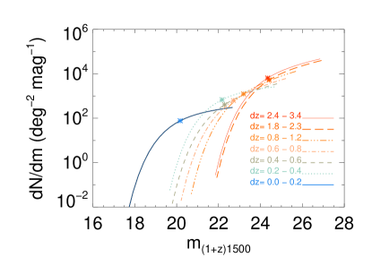
Figure 1: Star-forming galaxy surface density as a function of redshift derived from the luminosity functions listed in Table 1.

We convert from the number per comoving volume to the number per square degree by multiplying by the comoving volume per solid angle, calculated at about the mid-point in each redshift interval.

$$m^{*}_{(1+z)1500}=M^{*}_{15}+2.5log{\left[\frac{(d_{l}(z)*10^{5})^{2}}{(1.+z)}\right]}.$$ (5)

Here $d_{l}(z)$ is the luminosity distance in Mpc, and $z$ is the redshift.

In Figure 1 we show the luminosity functions listed in Table 1 recast into the number of galaxies per unit magnitude per square degree. Each curve has an $*$ to indicate the location of the characteristic magnitude $m^{*}_{(1+z)1500}$ where the Schechter function makes the transition from the exponential cutoff in galaxy counts at the bright end of the luminosity function to the power law extension of the faint end. The interval for the abscissa of each curve spans 5 mag (a factor of 100 in flux) centered on $m^{*}_{(1+z)1500}$. The figure is useful for estimating the number of targets within a given patch of sky down to an instrument’s brightness limit.

$$m^{*}_{(1+z)900}=m^{*}_{(1+z)1500}+\delta m^{1500}_{900}+\delta m_{esc}.$$ (6)

where $\delta m_{esc}=2.5\log{f^{e}_{900}}$, $\delta m^{1500}_{900}=2.5\log{F^{i}_{1500}/F^{i}_{900}}$, determined from the STARBURST99 (Leitherer et al., 1999, 2014, hereafter SB99) intrinsic SED described in § 3.2. Conveniently, in the rotating stellar evolution model , $F^{i}_{1500}/F^{i}_{900}\approx$ 1. This ratio is relatively insensitive to age in constant star-formation models. In the older, non-rotating SB99 models the range is 1.5 $\lesssim F^{i}_{1500}/F^{i}_{900}\lesssim$ 3 for ages 10 – 900 Gyr. A factor of 2 in the flux ratio amounts to $\delta m^{1500}_{900}=2.5\log{F^{i}_{1500}/F^{i}_{900}}\approx 0.75$.

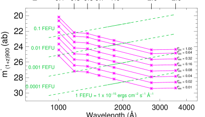
Figure 2: Estimate of each luminosity function’s characteristic magnitude, $m^{*}_{(1+z)900}$, as a function of redshift and assumed $f^{e}_{900}$ escape fraction just shortward of the edge Lyman edge. These estimates do not include IGM attenuation.

The estimates for $m^{*}_{(1+z)900}$, shown as magenta lines in Figure 2, are based on the rotating evolutionary models. They may be adjusted to adhere to the older models by shifting the ordinate by the preferred $\delta m^{1500}_{900}$ (= 0 for the rotational models). Likewise, offsets to account for differences in dust attenuation between 1500 and 900 Å may also be applied.

We have neglected here the stochastic attenuation expected from intervening neutral hydrogen absorption systems associated with the IGM. We will quantify the effects of this additional attenuation in § 4.

The estimate for $m^{*}_{(1+z)900}$ at a given $f^{e}_{900}$ is intended to provide guidance for detecting LyC emission at the most attenuated wavelength, just over the Lyman edge. The green dashed contours in Figure 2 indicate the flux levels $F_{(1+z)900}$ in units of femto erg flux units (1 FEFU = 10^-15 erg cm^-2 s^-1 Å^-1 ), which was roughly the background limit for the Far Ultraviolet Spectroscopic Explorer (FUSE). Current space-based UV background limits are $\sim$ 1 - 1000 times lower and will be discussed in § 4.1.2.

It should be kept in mind that $f^{e}_{900}$ is not a measure of the ratio of the total number of ionizing photos that escape to the total number that are emitted. In the following section we show that while the LyC flux in the relatively narrow wavelength range just shortward of the Lyman edge can be essentially zero, the fraction of escaping continuum photons integrated over the entire LyC emitting region, from the edge into the extreme UV (EUV), is significantly greater than zero.

3 Lyman Drop-ins

The abrupt drop-out in flux shortward of the LyC is a useful diagnostic for the photometric identification of star-forming galaxies (Steidel et al., 1995). The wavelength of the band where the flux drops out provides a constraint on the redshift. The technique was originally developed using ground-based surveys, which can efficiently identify objects at redshifts $z\approx$ 3 – 4. Lyman drop-outs at these redshifts are commonly referred to as Lyman Break Galaxies (LBGs). Cooke et al. (2014) have emphasized that the standard LBG technique is biased toward star-forming galaxies with zero detectable flux in the LyC, i.e. when line of sight column densities of $N_{HI}>>1\times$10¹⁸ cm^-2. For $N_{HI}\sim 1\times$10¹⁸ cm^-2 the drop-out does not extend completely throughout the EUV range, so we expect to find a class of star-forming galaxies that we call Lyman “drop-ins” as described below.

3.1 H I, He I, He II CGM transmission model

In principal, the shape of the continuum emission shortward of the Lyman edge contains a great deal of information regarding the distribution of ionization states for hydrogen and helium, and the distribution of dust along those unresolved line of sight(s) through an individual galaxy’s CGM favoring the escape of LyC radiation. The attenuation at each photoionization edge increases sharply followed by a relatively gentle recovery, varying approximately as $\propto(\frac{\lambda}{\lambda_{e}})^{3}$, where the $\lambda_{e}$ for H I, He I, and He II are 911.75, 504.26, and 227.84 Å, respectively.

In general, the transmission below the Lyman edge is a exponential function of the sum of dust, neutral hydrogen, neutral helium, and singly ionized helium optical depths,

$$T_{CGM}(\lambda)=\exp[{-\tau_{d}(\lambda)-\tau_{HI}(\lambda)-\tau_{HeI}(\lambda)-\tau_{HeII}(\lambda)}],$$ (7)

where the various optical depths are products of the column densities and cross-sections for each species, $\tau_{x}(\lambda)=N_{x}\sigma(\lambda)$. For the hydrogen and helium photoionization cross-sections we use the analytic fits from Verner et al. (1996), which differ slightly from the $\lambda^{3}$ relation. For the H I, He I, and He II resonance line cross-sections calculations we use the wavelengths and oscillator strengths for the 1 $<n<$ 79 lines of each species found in the online repository complied by Kurucz in CD-ROM 23.

We calculated the total optical depth template for each species, following a procedure used by McCandliss (2003), wherein Voigt profiles were generated for individual lines with fine enough sampling and range to resolve the doppler core and return the optical depth in the damping wing to near 0. Individual line profile optical depths were interpolated onto an common grid spanning the entire wavelength range of interest, for summation with all other lines and photoionization cross-sections. The doppler velocity was set to $b$ = 35 km s^-1, as is commonly assumed (Madau, 1995; Inoue & Iwata, 2008; Inoue et al., 2014) and is sufficient for our flux estimation exercise; however, it should be kept in mind that observations of the differential distribution of $b$ have been matched to $\frac{dN}{db}=\frac{4b^{4}_{\sigma}}{b^{5}}\exp(-(\frac{b_{\sigma}}{b})^{4})$ with $b_{\sigma}\approx$ 26 km s^-1 (Hui & Rutledge, 1999). How $\frac{dN}{db}$ varies with redshift is an open question.

The relative contributions of the three species are linked through the cosmic abundance of helium by number and imposed assumptions for the neutral fractions with respect to the total for the element (molecular hydrogen is neglected); i.e., $N^{tot}_{H}=N_{HI}+N_{HII}$, $N^{tot}_{He}=N_{HeI}+N_{HeII}+N_{HeIII}$ and $N^{tot}_{He}$ = 0.08 $N^{tot}_{H}$. The independent variables are the column of H I, its neutral fraction, $\chi_{HI}\equiv\frac{N_{HI}}{N^{tot}_{H}}$, and the helium neutral fraction, $\chi_{HeI}\equiv\frac{N_{HeI}}{N^{tot}_{He}}$.

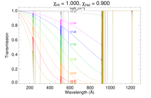
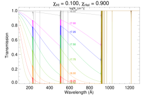
Figure 3: LyC transmission functions for $\log{N_{HI}(cm^{-2})}$ = 16.00, 17.00, 17.25, 17.50, 17.75, 18.00, 18.25, 18.50 that span the transition from optically thin to thick at the Lyman edge. Top – $\chi_{HI}$ =1, $\chi_{HeI}$ = 0.9. Bottom – $\chi_{HI}$ =0.1, $\chi_{HeI}$ = 0.9.

.

In Figure 3 we show two sets of transmission models, having ($\chi_{HI}$, $\chi_{HeI}$) = (1.0, 0.9), and (0.1, 0.9), top and bottom, respectively. The overall blackness of $f^{e}_{900}$ is set by the $N_{HI}$ column density, but total fraction of escaping LyC photons is set by the ionization state hydrogen relative to that of helium. The strength of the neutral and ionized helium edges becomes enhanced for $\chi_{HI}<$ 1.

The nature of dust attenuation in a highly ionized density bounded medium below the hydrogen Lyman edge is highly uncertain, so we have neglected it here. This should not be too serious, as the extinction near the Lyman edge in the canonical Milky Way model of Weingartner & Draine (2001, their Figure 14) is $N_{HI}/A(912)\approx$ 2.4 $\times$ 10²⁰ cm^-2 mag^-1. For $N_{HI}$ = 10¹⁸ cm^-2 this yields $A(912)$ =0.0042, so with $\tau_{d}(912)=A(912)/1.086$, we estimate a miniscule effect on transmission at the edge of $\exp{(-\tau_{d}(912))}$ = 0.996. However, if the dust abundance follows the total hydrogen instead of just H I, then $\tau_{d}$ will be higher.

In principal, a proper accounting of the neutral and ionized gases could lead to important observational insights into the temperature of the CGM along with the survivability and attenuation properties of dust grains with respect to the total gas content in LyC-leaking environments.

3.2 Intrinsic SB99 Star Formation Model

We employ here an SB99 spectral synthesis model, forming stars at a continuous rate of 1 $M_{\odot}$yr^-1 (Leitherer et al., 1999, 2014) for the intrinsic SED. We specified a Kroupa initial mass function, which has double power law exponents of -1.3, over the mass interval from 0.1 $<M_{\odot}<$ 0.5, and -2.3 for 0.5 $<M_{\odot}<$ 100. We also chose the Geneva evolutionary tracks with rotation at 40% of the break-up velocity (v0.4 models) and solar metallicity were also selected. After about 10 Myr the number of ionizing photons emitted by this model below the Lyman edge saturates at a rate of $\log{[Q_{0}(s^{-1})]}\sim$ 53.4 (Leitherer et al., 1999). The mass at this point is 10${}^{7}M_{\odot}$.

3.3 SB99 models with CGM attenuation

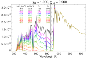
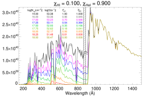
Figure 4: LyC drop-ins with ($\chi_{HI}$, $\chi_{HeI}$) as in Figure 3. SB99 v0.4 evolution model attenuated with the transmission functions in Figure 3. For $\log{N_{HI}(cm^{-2})}>$18 the escape fraction measured at 900 Å $f^{e}_{900}<<$1%, yet the integrated fraction of ionizing photons that escape, $f^{e}_{LyC}$, is significantly greater than $f^{e}_{900}$. The top panel shows a relatively smooth Lyman drop-in at $\log{N_{HI}(cm^{-2})}=$18. The bottom panel shows a double drop-in.

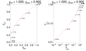
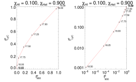
Figure 5: Integrated fraction of escaping LyC photons, $f^{e}_{LyC}$ on ordinate, escape fraction at 900 $f^{e}_{900}$on abscissa. Top–bottom order for ($\chi_{HI}$, $\chi_{HeI}$) as in Figure 3. Left linear–linear. Right log–log. The relationship is decidedly non-linear. Top to bottom shows varying degrees of significant escape even when $f^{e}_{900}$ has become black.

In Figure 4 we show the effect of attenuating the SB99 model with the transmission functions depicted in Figure 3. The shape of the continuum emitted below the Lyman edge, and hence the number of ionizing photons that ultimately escape from a star-forming region, is linked to the ionization state of hydrogen and helium in the surrounding column of gas. There is very little intrinsic stellar flux emitted below the He II edge at 228 Å, so the inclusion of He II has little effect on the overall total escape fraction. However, it would become important for the harder SEDs typical of quasars and AGN.

The top panel has ($\chi_{HI}$, $\chi_{HeI}$) = (1.0, 0.9), where we have assumed that helium is slightly ionized for the purpose of showing the location of the He II Lyman series. This model shows signs of a slight break shortward of the He I ionization edge at 504 Å, but overall it exhibits a relatively smooth Lyman drop-in with decreasing wavelength. In the bottom panel ($\chi_{HI}$, $\chi_{HeI}$) = (0.1, 0.9), so the break shortward of 504 Å is strengthened by the lower H I abundance with respect to He I, causing a Lyman ”double drop-in” to appear in the EUV region. The strength of the He I break with respect to the H I break becomes more enhanced as $\chi_{HI}$ decreases.

In each figure we have tabulated logarithms of the H I column density, the rate of ionizing photon production, the escape fraction integrated over the entire EUV band, $f^{e}_{LyC}$, and the escape fraction of ionizing photons in the narrow 20 Å wide region shortward of the Lyman edge, $f^{e}_{900}$. The table entries are color-coded to the spectra.

In Figure 5 we show that the relationship between $f^{e}_{LyC}$ and $f^{e}_{900}$, (logarithmic scales left and liner scales right) is decidedly nonlinear. We have overplotted an interpolation formula of the form

$$f^{e}_{LyC}=\frac{(f^{e}_{900})^{\zeta_{1}}+(f^{e}_{900})^{\zeta_{2}}+\epsilon}{(2+\epsilon)},$$ (8)

where ($\zeta_{1},\zeta_{2}$, and $\epsilon$) = (0.25, 0.75, 0.018) and (0.37, 0.95, 0.0011), for ($\chi_{HI}$, $\chi_{HeI}$) = (1.0, 0.9) and ($\chi_{HI}$, $\chi_{HeI}$) = (0.1, 0.9), respectively.

In all cases a column density $\log{N_{HI}(cm^{-2})}$ = 18 produces essentially zero flux at the edge, yielding an edge escape fraction of $f^{e}_{900}$= 0.003, yet the integrated escape fraction is 13 and 6%, for the two cases, respectively. Using the interpolation formulae, we find that for the Lyman edge escape fractions used in Figure 2, where $f^{e}_{900}$ = (0.01, 0.02, 0.04, 0.08, 0.16, 0.32, 1.00), the corresponding integrated escape fraction is $f^{e}_{LyC}$ = (0.18, 0.22, 0.27, 0.35, 0.45, 0.59, 1.00) and (0.10, 0.13, 0.18, 0.24, 0.34, 0.50, 1.00) for the two cases, respectively.

We conclude that measurements of the Lyman edge escape fraction, $f^{e}_{900}$, only provide, at best, lower limits to the the true integrated fraction of escaping ionizing photons, and generally offer poor representations of the total number of ionizing photons that escape. The tables in Figures 4 show that LBGs may emit significant amounts of LyC radiation, at the level of 5 to 1%, even if the optical depth at the edge is $\approx$ 10 ( $\log{N_{HI}(cm^{-2})}$ = 18.25). By way of example, we note that Izotov et al. (2016a) found an edge escape fraction $f^{e}_{900}$ = 0.08. Using Eq. 8, we derived an integrated escape fraction of $f^{e}_{LyC}$ = 0.35 or 0.25 for our two cases, respectively. This suggests that the “f-escape” problem might not be as bad as it seems. The only definitive way to rule this out is through deep UV observations in the redshifted rest frame of the EUV in an attempt to observe the LyC drop-in.

In the next section we address the observability of of the Lyman drop-ins in the face of the steadily increasing mean optical depth of the IGM with increasing redshift.

4 Redshifted models, including mean IGM transmission

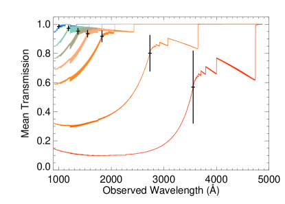
Figure 6: Mean IGM transmission functions for redshifts $z$ = (0.1, 0.3, 0.5, 0.7, 1.0, 2.0, 2.9). Computed from the ($\chi_{HI}$, $\chi_{HeI}$) = (1.0, 0.9) model. The vertical bar indicates the level of expected variation at the edge as found in Monte Carlo study of IGM absorbers distributed over a range of column densities from LAF to DLA with a piecewise break at the LL transition Inoue & Iwata (2008).

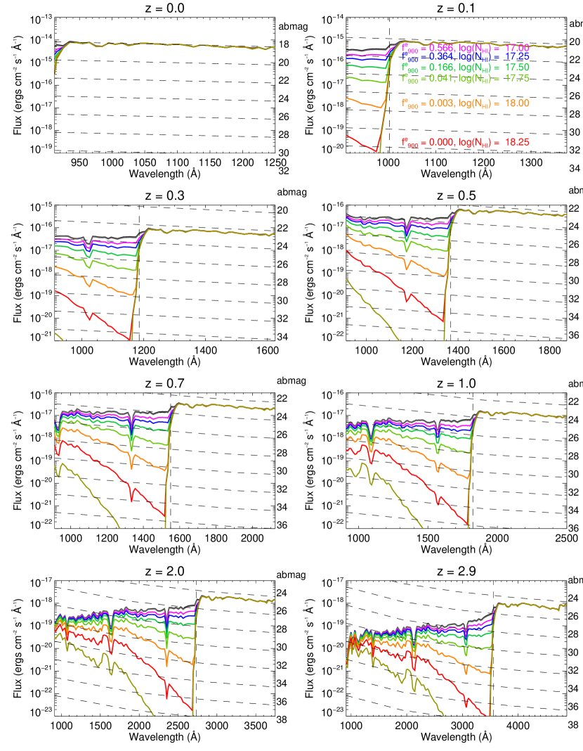
Figure 7: Redshifted ($\chi_{HI}$, $\chi_{HeI}$) = (1.0, 0.9) model with logarithmic scaling, showing LyC drop-in towards shorter wavelengths. Contours of constant abmag appear as dashed lines. Column density colors as in Figure 4. The edge escape fractions are $f^{e}_{900}$ ( 0.000, 0.003, 0.041, 0.166, 0.364, 0.566, 0.945) for ( red, orange, light green, green, blue, violet, and grey) respectively.

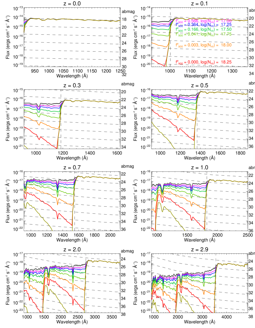
Figure 8: Redshifted ($\chi_{HI}$, $\chi_{HeI}$) = (0.1, 0.9) model with logarithmic scaling. The $z$ = 2.0 and 2.9 models show the pronounced double drop-in structure is severely depressed, but the structure survives albeit at a difficult to detect level. Colors and edge escape fractions as in Figure 7.

We have thus far not included attenuation of the escaping LyC due to resonant scattering and photoelectric absorption (photoionization) from discrete collections of intervening clouds in the IGM. Here we use the rest frame LyC transmission models described in § 3.1 to compute the mean transmission of the IGM as a function of the fiducial redshifts in Table 1.

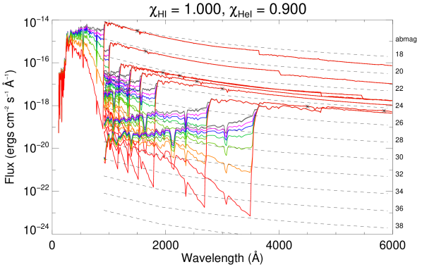
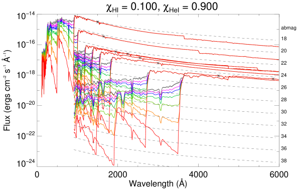
Figure 9: Column density colors as in Figure 4, but the lowest column 18.5 is omitted. Asterisks mark (1+$z$)1500 Å. Contours of constant abmag appear as dashed lines. Top – ($\chi_{HI}$, $\chi_{HeI}$) = (1.0, 0.9) model with logarithmic scaling. Bottom – ($\chi_{HI}$, $\chi_{HeI}$) = (1.0, 0.9).

The mean transmission function is derived from a mean optical depth (Paresce et al., 1980; Madau, 1995; Inoue et al., 2014), expressed here as a numeric integral

$$<\tau(\lambda)>=\sum_{i=0}^{L}\sum_{j=0}^{M}\left(\frac{\partial^{2}n}{\partial{N_{HI}}\partial{z}}\right)_{i,j}(1-e^{-\tau(\lambda_{o})})\Delta z_{i}\Delta N_{j}.$$ (9)

Here the observed wavelength is related to the rest frame wavelength by $\lambda_{o}=\lambda_{r}(1+z_{i})$. The optical depth is $\tau(\lambda_{o})=\tau_{HI}(\lambda_{o})+\tau_{HeI}(\lambda_{o})+\tau_{HeII}(\lambda_{o})$. The redshift range from 0 $\leq z_{i}\leq z_{L}$ is in fixed increments of $\Delta z_{i}$ =0.0005. The logarithm of the column densities range from 12.3 $\leq\log({N_{j}})\leq$ 22 in variable increments of $\Delta N_{j}=N_{j+1/2}-N_{j-1/2}$ with 0 $\leq j\leq M$ .

The differential distribution of the number of discrete absorbers with respect to H I column density and redshift, $\frac{\partial^{2}n}{\partial{N_{HI}}\partial{z}}$, is typically characterized by a piecewise continuous function in redshift and column density (c.f. Madau, 1995; Inoue et al., 2014). There are three basic H I absorption regimes: the Ly$\alpha$ forest regime (LAF), $\log{N_{HI}(cm^{-2})}\lesssim$ 17; the Lyman limit (LL) regime, 17 $\lesssim\log{N_{HI}(cm^{-2})}\lesssim$ 20, and the damped Ly$\alpha$ (DLA) regime, $20\lesssim\log{N_{HI}(cm^{-2})}$.

We employ the $\frac{\partial^{2}n}{\partial{N_{HI}}\partial{z}}$ described by Inoue et al. (2014), which uses a ”Schechter-like” distribution function for the column density multiplied by a piecewise-continuous multiple power law distribution to describe the evolution in redshift. The distribution function is broken down into the sum of two different products, which in combination reasonably agrees with the evolution of H I absorption systems from the LLA to DLA regimes as detailed in the literature (Weymann et al., 1998; Prochaska et al., 2005, 2010; Ribaudo et al., 2011; Noterdaeme et al., 2012; Fumagalli et al., 2013; Kim et al., 2013; O’Meara et al., 2013; Prochaska et al., 2014). We note that the Inoue et al. (2014) distribution function produces a mean transmission that is generally less aggressive than that produced by the distribution function used by Madau (1995), even though it does not include a contribution from DLAs.

The mean IGM transmission functions in the observers frame, $T_{IGM}(\lambda_{o})=\exp{<-\tau(\lambda)>}$, are plotted in Figure 6 for $z$ = (0.1, 0.3, 0.5, 0.7, 1.0, 2.0, 2.9). These transmission functions were computed from the ($\chi_{HI}$, $\chi_{HeI}$) = (1.0, 0.9) model. We emphasize that they are just mean relationships. Significant stochastic deviations are expected along any given line of sight. We give an indication of the level of such variations at the Lyman edge by overplotting the 68% deviations found by Inoue & Iwata (2008, their Figure 8) in a Monte Carlo simulation of IGM absorbers distributed over a range of column densities from LAF to DLA with a piecewise break at the LL transition. The appearance, or absence, of an LL system in the Monte Carlo simulation drives much of the expected transmission stochasticity. We see that while the mean attenuation is significant at $z$ =2.9, reaching a lower trough of $\approx$ 15% at 2000 Å, it is by no means complete. The transmission at the Lyman edge for each redshift is $T(z)$ = (0.98, 0.97, 0.95, 0.94, 0.92, 0.80, 0.57), which translates to a decrease in abmag at the respective edges of $\delta m^{*}_{(1+z)900}$ = (0.02, 0.03, 0.05, 0.07, 0.09, 0.24, 0.61).

In Figures 7, 8 and 9 we show the result of applying $T_{IGM}(\lambda_{o})$ to the ($\chi_{HI}$, $\chi_{HeI}$) = (1.0, 0.9) and ($\chi_{HI}$, $\chi_{HeI}$) = (0.1, 0.9) luminosity density models respectively. using abmag = -2.5$\log{F_{\nu}}$-48.6 and substituting $F_{\nu}=\frac{\lambda^{2}}{c}F_{\lambda}$, we determined the flux, $F_{(1+z)1500}$ in the observer’s frame from $m^{*}_{(1+z)1500}$ in Table 1, such that

$$\log(F_{(1+z)1500})=\frac{m^{*}_{(1+z)1500}+5\log{[(1+z)1500]}+2.408}{-2.5},$$ (10)

and found a scale factor, $M_{7}$, matching the redshifted SB99 luminosity density at luminosity distance $d_{l}(z)$ to the observed SED $F_{(1+z)1500}$ such that

$$F_{\lambda_{o}}=M_{7}\left(\frac{L_{(1+z)\lambda_{r}}}{4\pi d_{l}^{2}(z)(1+z)}\right).$$ (11)

Here the luminosity distance $d_{l}(z)$ is in cm $M_{7}=$ [0.8, 1.1, 3.2, 4.4, 5.6, 6.9, 13.7] for the fiducial redshifts in Table 1. The $z=0$ model is fixed to $m_{1500}$ = 18.0, with $M_{7}=1$ at a distance of $d_{l}$ = 177 Mpc. The mean transmission function was applied as a uniform screen to $F_{\lambda_{o}}$. The CGM transmission is applied to $L_{\lambda_{r}}$ in the rest frame prior to redshifting. Lines of constant abmag are overplotted on the figures.

4.1 LyC Detection Requirements

The results of the previous section show that detection and quantification of the fraction of LyC flux escaping from star-forming galaxies out to $z\sim$ 3 will be a formidable, but not insurmountable, challenge for future space observatories. Moreover, they are consistent with the paucity of detections to date.

4.1.1 Current Capabilities

Examining the $z=$ 0.1 models, we see that very little of the LyC region peeks out below $\sim$ 1000 Å. The Cosmic Origins Spectrograph (COS) on the Hubble Space Telescope (HST) has limited sensitivity in this bandpass ($A_{eff}\sim$ 10 cm^-2), with a background equivalent flux (BEF) of $\sim$ 10^-15 erg cm^-2 s^-1 Å^-1  $\sim$ 20 abmag (McCandliss et al., 2010; Redwine et al., 2016). Galaxies brighter than this are in the region of the exponential falloff in the luminosity function, so they become increasingly rare with increasing luminosity. Characteristic galaxies with edge escape fractions $f^{e}_{900}<0.4$, will have an attenuated edge flux more than an order of magnitude lower than the COS BEF. Consequently, they will be background limited, requiring extraordinarily long integration times to detect with confidence. We can expect to detect only a handful of such objects over the lifetime of COS. The three detections by Leitherer et al. (2016) at $z\approx$ 0.04 had edge fluxes $\sim$ 1 to 2 $\times$ 10^-15 erg cm^-2 s^-1 Å^-1 .

The situation is somewhat more favorable at $z$ = 0.3, 0.5, and 0.7, where the $m^{*}_{(1+z)1500}$ are quite similar ($m^{*}_{1950}$, $m^{*}_{2250}$, $m^{*}_{2550}$ = 22.3, 22.4, 22.7) and the LyC region extends shortward of $\sim$ 1200, 1350, and 1550 Å, respectively, into a wavelength region where the COS effective area $A_{eff}>$ 1000 cm^-2. Although the $m^{*}_{(1+z)1500}$ for galaxies at these redshifts are nearly an order of magnitude fainter than at $z$ = 0.1, the COS BEF is much lower than at $z=$ 0.1 ($\sim$ 10^-17 to 10^-18 erg cm^-2 s^-1 Å^-1  $\sim$ 25 to 27.5 abmag – depending on orbital attitude and solar activity), thus allowing for more efficient observing programs to be constructed. Still, the background limit is reached for characteristic galaxies at $f^{e}_{900}\approx$ 0.04 to 0.16. The depth of such observations will be limited and robust statistical samples difficult to come by, especially for $z$ = 0.5 and 0.7, where the number density is nearly 4 times lower. Nevertheless, the spectral baseline is relatively longer, which along with the higher effective area favors the detection of LyC drop-ins toward these higher redshifts.

For galaxies at $z\approx$ 1 the detection of escaping LyC with COS becomes even more difficult, as the unattenuated LyC region is of order the BEF. This was also the case for LyC leak photometric searches conducted using GALEX. The FUV ($\lambda_{eff}$ = 1528 Å, $\Delta\lambda$ =1344 - 1786) and NUV ($\lambda_{eff}$ = 2271 Å, $\Delta\lambda$ =1771 - 2831 channels on GALEX straddle the break for objects at a redshift of $z\approx$ 1.1. The GALEX  5$\sigma$ flux limit was $\sim$25 to 24 abmag for 30 ks integration in the FUV and NUV, respectively (Morrissey et al., 2005). In the NUV a $z$ = 1 characteristic galaxy is $\sim$23 abmag, while the unattenuated FUV SED ($f^{e}_{900}$ =1) has $\sim$25 abmag at 1530 Å; this is too faint for robust detections at near unity escape fraction. These limits are consistent with the Cowie et al. (2009) analysis of deep GALEX exposures of the GOODS-N field with spectroscopic redshifts, where they found no objects with FUV $<$ 25 for redshifts of $z>0.6$. We conclude that the limiting flux of GALEX was not low enough to adequately survey LyC leakage at a redshift of $z\gtrsim$ 1.

Observations by Siana et al. (2007) using the Space Telescope Imaging Spectrograph (STIS) and Advanced Camera for Surveys Solar Blind Channel (ACS/SBC) found no detections in deep far-UV observations around 1600 Å  of 21 HUDF objects with known spectroscopic redshifts 1.1 $<z<$ 1.5. The $3\sigma$ limits in the ACS/SBC F150LP channel were estimated to be $\approx$28 abmag. Their median abmag at 1500(1+1.3) = 3450 Å was 24.5, which is about 1 mag fainter than our characteristic magnitude at $z$ = 1. The non-detection to a 28 abmag limit at observer frame 1600 Å implies a $\log{N_{HI}(cm^{-2})}\gtrsim$ 17.75, yielding a $f^{e}_{900}$ $\sim$ 0.04 (an integrated 0.17 $<f^{e}_{LyC}<$ 0.26). These values compare fairly well to their stacked limit of $f_{esc,rel}<$ 0.08 evaluated at 700 Å in the rest frame.

Hubble Deep UV (HDUV) imaging of the GOODS-north and -south fields, using the Wide-Field Camera 3 (WFC3) filters F275W and F336W and redshifts supplied by 3D-HST Grism, to explore the redshift range $z\sim$ 2–3. The 5$\sigma$ detection limit was $\sim$ 28 abmag. The candidate leakers were estimated to have $f_{esc}>$ 0.6. This result is consistent with our $z$ = 2 and 2.9 calculations, showing that a characteristic galaxy at these redshifts with an abmag of 28 in the LyC will have $f^{e}_{900}>$ 0.4 at $z$ = 2 and $f^{e}_{900}>$ 0.6 at $z$ = 3.

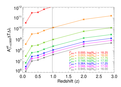
Figure 10: The product of effective area $A_{eff}(\lambda)$, observing time $\Delta T$, and bandwidth $\Delta\lambda$ required to detect flux from a characteristic galaxy, attenuated by a $\log{N_{HI}(cm^{-2})}$ = [18.25, 18.00, 17.75, 17.50, 17.25, 17.00, 16.00], in the wavelength region just over the Lyman edge, with a signal to noise of 5. The corresponding edge escape fractions are $f^{e}_{900}$ = [0.000, 0.003, 0.041, 0.166, 0.364, 0.566, 0.945] in color code of [red, orange, light green, green, blue, violet, grey]. The example given in the text (Eq. 12) is marked with black horizontal and vertical lines.

4.1.2 Future Capability Requirements

It is clear from Figure 2 that if we are to achieve the goal of statistically significant determination of LyC luminosity function evolution wherein we probe down to $f^{e}_{900}\approx$ 0.01 out to a redshift of 3, then we need to reach an abmag from 25 to 30 for the characteristic objects in the redshift range from 0.1 $<z<$ 2.9 . This corresponds to a flux range of $F_{(1+z)900}\sim$ 10^-17 to 10^-20 erg cm^-2 s^-1 Å^-1 . The luminosity function spans a range of $\approx\pm$ 2.5 mag about the characteristic value, so the flux range will need to be another factor of 10 lower to obtain adequate numbers of low-luminosity objects.

By way of example, if we assume a limiting flux requirement of $F^{lim}_{1800}$ =2 $\times$ 10^-20 erg cm^-2 s^-1 Å^-1  at a 1800 Å as a representative goal for $\sigma$ = 5 of edge detection with a $f^{e}_{900}\gtrsim$ 0.003 for faint-end objects at $z\approx$ 1, then we arrive at the following criteria for the product of effective area ($A^{eff}_{1800}$, observing time $\Delta T$, and $\Delta\lambda$ spectral bandwidth, assuming negligible background):

$$A^{eff}_{1800}~{}\Delta T~{}\Delta\lambda=\frac{\sigma^{2}}{F_{1800}/E_{1800}}=1.3\times 10^{10}{\rm cm^{2}\;s\;\AA},$$ (12)

where $E_{1800}$ is the photon energy at 1800 Å. This formula assumes that there is negligible background. It may be used for estimating effective area, observing time, and bandwidth requirements for photometric and spectroscopic applications. In Figure 10 we show the area-time-bandwidth product Lyman edge detection requirement for $\log{N_{HI}(cm^{-2})}$ = [18.25, 18.00, 17.75, 17.50, 17.25, 17.00, 16.00] as a function of redshift.

4.1.3 Target Sample Goals

there are $\sim$ 300 objects per unit magnitude per square degree at $z=$ 0.1 at the faint-end. By 0.3 $z=$ 0.3 the faint end areal density are $\sim$ 3000 objects per unit magnitude per square degree, being flat out to $z=$ 1. For $z=$ 2 the areal density at the faint end rises to $\sim$ 50,000 objects per unit magnitude per square degree.

The construction of high-fidelity luminosity functions places a requirement on sample size, where 25 objects per luminosity bin per redshift interval will yield an approximate rms deviation of $\sim$ 20% for each point. Luminosity range should be   2 - 3 orders of magnitude with $\sim$ 20 to 40 bins covering 10 redshift intervals. Redshifts are required for each object. This suggests an observing program with 500–1000 objects per redshift interval, yielding 5000–10,000 objects in total.

The development of a wide-field multi-object spectroscopic (MOS) capability and complementary photometric observations will be essential to providing these samples. Angular coverage requirements will be driven by low-redshift objects, which have lower areal number densities than higher-redshift objects, while observing time requirements will be driven by the faintest objects.

4.2 Observing Strategies

Spectroscopy and photometry provide complementary approaches to this problem. Spectroscopy offers an opportunity to examine in detail the variation of the flux escaping at wavelengths below the Lyman edge along with the compositional properties of the objects. Photometry can go deeper and offer higher spatial resolution at the expense of spectral information. Spectroscopy provides an avenue for training photometry.

A comprehensive program will incorporate photometry into the search for candidates and the deep probe of the faint end of the LyC luminosity function, while low-resolution precision spectroscopy will be used to characterize the shape of the LyC in a search for drop-ins, offering clues for the total ionizing photon budget and potentially dust attenuation in a completely unexplored bandpass. Spectral multiplexing over several square arcminutes will be of great importance for acquiring statistically significant samples in a reasonable amount of observing time.

These observations should be complemented by medium- to high-resolution ($R\sim$ 10,000 - 50,000) spectroscopy longward of the Lyman edge, providing a baseline assessment of intervening H I and metallic absorption systems associated with the CGM and IGM. Such observations, supported by spatially resolved imaging at the scale of 10 to 100 pc, can be used to account for the partial covering of emission regions, wherein the uniform screen assumption assumed here could be relaxed in favor of the informed modeling of foreground sources using measured superpositions of H I columns and metallic absorption distributions. This is especially important for determining the randomly distributed IGM attenuation prior to quantifying the actual escape from the CGM for the higher-$z$ objects. Success at high $z$ is likely to rely on the identification of “lucky sight-lines” aided by gravitational lens and/or a several $\sigma$-low deviation from the average number of obscuring line of sight IGM absorption systems.

5 Conclusion

Measurements of $f^{e}_{LyC}$ at $z\lesssim$ 3 across all types of star-forming galaxies are crucial to informing our understanding of how the universe came to be ionized. UV observations, far and near, provide the most direct path to the spatially resolved detection of ionizing radiation, and the opportunity to characterize the physical state of galactic environments that favor LyC escape.

The primary purpose of this work is to provide estimates of the flux in the LyC from star-forming galaxies, as functions of escape fraction and redshift. quantifying science return, defining technical requirements, and observing strategies for future large, medium, and small scale missions to be considered by the Astrophysics Decadal for 2020. A model has been developed based on a uniform foreground screen of H I, He I, and He II, attenuating a young continuous star-forming object with fluxes at (1+z)1500 Å scaled to reproduce the characteristic apparent magnitudes of the Arnouts et al. (2005) luminosity functions. The uniform screen model has as free parameters the ionization fractions of H and He ($\chi_{HI}$, $\chi_{HeI}$), wherein the ratio of H to He is set to the cosmic abundance. We also account for the mean attenuation by power law distributions of Ly$\alpha$ forest, LL, and DLA systems associated with the IGM as a function of increasing redshift.

We caution that the escape fraction measured just below the Lyman edge ($f^{e}_{900}$) at 911.8 Å provides only a lower limit to the fraction of LyC photons that escape as integrated over the entire EUV region ($f^{e}_{LyC}$). For 18.5 $>\log{N_{HI}(cm^{-2})}>$17.9, the Lyman edge can appear black (essentially zero) yet the integrated escape fraction can range from 1 to 20%, depending on the choice of ionization fractions ($\chi_{HI}$, $\chi_{HeI}$).

More accurate assessments of the integrated escape fraction could be made from spectroscopic observations that resolve the recovery of flux $\propto(\frac{\lambda}{\lambda_{e}})^{3}$; a phenomena that we have dubbed Lyman “drop-ins”. Observations of the LyC spectral shape could provide, in principle, the following: enhanced fidelity to the determination of the contribution of star-forming galaxies to the MIB; important observational insights into the temperature of the CGM and IGM; and constraints on the survivability and attenuation properties of dust grains with respect to the total gas content in LyC-leaking environments.

The uniform screen model adopted here is considerably simpler than the more realistic case of an undulating, highly discontinuous and chaotic “unity H I optical depth” surface of the CGM surrounding a star-forming galaxy, which must have a $\tau$ low enough for LyC radiation to escape. The model should be thought of as a kind of ensemble average of the galaxy’s partially covered star-forming regions, wherein much of the total star-formation may be buried by a more heavily attenuating ISM.

We suggest a strategy of high spectral and spatial resolution observations in the region longward of the Lyman edge, to guide assessment of the line of sight geometry in coordination with a spectroscopic determination of the degree of partial covering, along with the identification of specific Ly$\alpha$ forest, LL, and DLA systems that may contribute to the attenuation of objects toward higher redshift. Such information will allow a relaxing of the simple uniform screen model in favor of more realistic radiative transfer models.

Achieving the goal of a statistically significant characterization of LyC luminosity function evolution out to $z\lesssim$ 3 can be carried out most efficiently with a wide-field multi-object spectroscopic survey supported by photometric observations. An instrument with an effective area, observing time, and spectral bandwidth product of 1.3 $\times$ 10¹⁰ cm² s Å at 1800 Å would be sufficient to carry out such a program to a redshift of $z=$ 1.

References

- Arnouts et al. (2005) Arnouts, S., Schiminovich, D., Ilbert, O., et al. 2005, ApJ, 619, L43
- Bahcall & Sargent (1967) Bahcall, J. N., & Sargent, W. L. W. 1967, ApJ, 148, L65
- Bechtold et al. (1987) Bechtold, J., Weymann, R. J., Lin, Z., & Malkan, M. A. 1987, ApJ, 315, 180
- Benson et al. (2013) Benson, A., Venkatesan, A., & Shull, J. M. 2013, ApJ, 770, 76
- Bland-Hawthorn & Maloney (1999) Bland-Hawthorn, J., & Maloney, P. R. 1999, ApJ, 510, L33
- Borthakur et al. (2014) Borthakur, S., Heckman, T. M., Leitherer, C., & Overzier, R. A. 2014, Science, 346, 216
- Bouwens et al. (2015) Bouwens, R. J., Illingworth, G. D., Oesch, P. A., et al. 2015, ApJ, 811, 140
- Cooke et al. (2014) Cooke, J., Ryan-Weber, E. V., Garel, T., & Díaz, C. G. 2014, MNRAS, 441, 837
- Cowie et al. (2009) Cowie, L. L., Barger, A. J., & Trouille, L. 2009, ApJ, 692, 1476
- Crighton et al. (2015) Crighton, N. H. M., Murphy, M. T., Prochaska, J. X., et al. 2015, MNRAS, 452, 217
- Danforth et al. (2016) Danforth, C. W., Keeney, B. A., Tilton, E. M., et al. 2016, ApJ, 817, 111
- Deharveng et al. (1997) Deharveng, J.-M., Faiesse, S., Milliard, B., & Le Brun, V. 1997, A&A, 325, 1259
- Dove & Shull (1994) Dove, J. B., & Shull, J. M. 1994, ApJ, 430, 222
- Dove et al. (2000) Dove, J. B., Shull, J. M., & Ferrara, A. 2000, ApJ, 531, 846
- Fan et al. (2006) Fan, X., Carilli, C. L., & Keating, B. 2006, ARA&A, 44, 415
- Fernandez-Soto et al. (2003) Fernandez-Soto, A., Lanzetta, K. M., & Chen, H.-W. 2003, MNRAS, 342, 1215
- Finkelstein et al. (2015) Finkelstein, S. L., Ryan, Jr., R. E., Papovich, C., et al. 2015, ApJ, 810, 71
- Fumagalli et al. (2013) Fumagalli, M., O’Meara, J. M., Prochaska, J. X., & Worseck, G. 2013, ApJ, 775, 78
- Gaikwad et al. (2017) Gaikwad, P., Khaire, V., Choudhury, T. R., & Srianand, R. 2017, MNRAS, 466, 838
- Gnedin et al. (2008) Gnedin, N. Y., Kravtsov, A. V., & Chen, H.-W. 2008, ApJ, 672, 765
- Hui & Rutledge (1999) Hui, L., & Rutledge, R. E. 1999, ApJ, 517, 541
- Inoue & Iwata (2008) Inoue, A. K., & Iwata, I. 2008, MNRAS, 387, 1681
- Inoue et al. (2014) Inoue, A. K., Shimizu, I., Iwata, I., & Tanaka, M. 2014, MNRAS, 442, 1805
- Izotov et al. (2016a) Izotov, Y. I., Orlitová, I., Schaerer, D., et al. 2016a, Nature, 529, 178
- Izotov et al. (2016b) Izotov, Y. I., Schaerer, D., Thuan, T. X., et al. 2016b, MNRAS, 461, 3683
- Kim et al. (2013) Kim, T.-S., Partl, A. M., Carswell, R. F., & Müller, V. 2013, A&A, 552, A77
- Kollmeier et al. (2014) Kollmeier, J. A., Weinberg, D. H., Oppenheimer, B. D., et al. 2014, ApJ, 789, L32
- Leitet et al. (2013) Leitet, E., Bergvall, N., Hayes, M., Linné, S., & Zackrisson, E. 2013, A&A, 553, A106
- Leitherer et al. (2014) Leitherer, C., Ekström, S., Meynet, G., et al. 2014, ApJS, 212, 14
- Leitherer et al. (2016) Leitherer, C., Hernandez, S., Lee, J. C., & Oey, M. S. 2016, ApJ, 823, 64
- Leitherer et al. (1999) Leitherer, C., Schaerer, D., Goldader, J. D., et al. 1999, ApJS, 123, 3
- Madau (1995) Madau, P. 1995, ApJ, 441, 18
- Madau & Haardt (2015) Madau, P., & Haardt, F. 2015, ApJ, 813, L8
- Madau et al. (1999) Madau, P., Haardt, F., & Rees, M. J. 1999, ApJ, 514, 648
- McCandliss (2003) McCandliss, S. R. 2003, PASP, 115, 651
- McCandliss et al. (2010) McCandliss, S. R., France, K., Osterman, S., et al. 2010, ApJ, 709, L183
- Morrissey et al. (2005) Morrissey, P., Schiminovich, D., Barlow, T. A., et al. 2005, ApJ, 619, L7
- Naidu et al. (2016) Naidu, R. P., Oesch, P. A., Reddy, N., et al. 2016, ArXiv e-prints, arXiv:1611.07038
- Noterdaeme et al. (2012) Noterdaeme, P., Petitjean, P., Carithers, W. C., et al. 2012, A&A, 547, L1
- Oke & Gunn (1983) Oke, J. B., & Gunn, J. E. 1983, ApJ, 266, 713
- O’Meara et al. (2013) O’Meara, J. M., Prochaska, J. X., Worseck, G., Chen, H.-W., & Madau, P. 2013, ApJ, 765, 137
- Paresce et al. (1980) Paresce, F., McKee, C. F., & Bowyer, S. 1980, ApJ, 240, 387
- Prochaska et al. (2005) Prochaska, J. X., Herbert-Fort, S., & Wolfe, A. M. 2005, ApJ, 635, 123
- Prochaska et al. (2014) Prochaska, J. X., Madau, P., O’Meara, J. M., & Fumagalli, M. 2014, MNRAS, 438, 476
- Prochaska et al. (2010) Prochaska, J. X., O’Meara, J. M., & Worseck, G. 2010, ApJ, 718, 392
- Razoumov & Sommer-Larsen (2010) Razoumov, A. O., & Sommer-Larsen, J. 2010, ApJ, 710, 1239
- Reddy et al. (2016) Reddy, N. A., Steidel, C. C., Pettini, M., Bogosavljević, M., & Shapley, A. E. 2016, ApJ, 828, 108
- Redwine et al. (2016) Redwine, K., McCandliss, S. R., Zheng, W., et al. 2016, PASP, 128, 105006
- Ribaudo et al. (2011) Ribaudo, J., Lehner, N., & Howk, J. C. 2011, ApJ, 736, 42
- Ricotti et al. (2002) Ricotti, M., Gnedin, N. Y., & Shull, J. M. 2002, ApJ, 575, 49
- Robertson et al. (2015) Robertson, B. E., Ellis, R. S., Furlanetto, S. R., & Dunlop, J. S. 2015, ApJ, 802, L19
- Schechter (1976) Schechter, P. 1976, ApJ, 203, 297
- Scott et al. (2004) Scott, J. E., Kriss, G. A., Brotherton, M., et al. 2004, ApJ, 615, 135
- Shapley et al. (2006) Shapley, A. E., Steidel, C. C., Pettini, M., Adelberger, K. L., & Erb, D. K. 2006, ApJ, 651, 688
- Shapley et al. (2016) Shapley, A. E., Steidel, C. C., Strom, A. L., et al. 2016, ApJ, 826, L24
- Sharma et al. (2016) Sharma, M., Theuns, T., Frenk, C., et al. 2016, MNRAS, 458, L94
- Shull et al. (2015) Shull, J. M., Moloney, J., Danforth, C. W., & Tilton, E. M. 2015, ApJ, 811, 3
- Siana et al. (2007) Siana, B., Teplitz, H. I., Colbert, J., et al. 2007, ApJ, 668, 62
- Smith et al. (1981) Smith, M. G., Carswell, R. F., Whelan, J. A. J., et al. 1981, MNRAS, 195, 437
- Smith et al. (1996) Smith, P. L., Esmond, J. R., Heise, C., & Kurucz, R. L. 1996, in UV and X-ray Spectroscopy of Astrophysical and Laboratory Plasmas, ed. K. Yamashita & T. Watanabe, 513–516
- Steidel et al. (2001) Steidel, C. C., Pettini, M., & Adelberger, K. L. 2001, ApJ, 546, 665
- Steidel et al. (1995) Steidel, C. C., Pettini, M., & Hamilton, D. 1995, AJ, 110, 2519
- Verner et al. (1996) Verner, D. A., Ferland, G. J., Korista, K. T., & Yakovlev, D. G. 1996, ApJ, 465, 487
- Weingartner & Draine (2001) Weingartner, J. C., & Draine, B. T. 2001, ApJ, 548, 296
- Weymann et al. (1998) Weymann, R. J., Jannuzi, B. T., Lu, L., et al. 1998, ApJ, 506, 1
- Wise et al. (2014) Wise, J. H., Demchenko, V. G., Halicek, M. T., et al. 2014, MNRAS, 442, 2560
- Worseck et al. (2014) Worseck, G., Prochaska, J. X., O’Meara, J. M., et al. 2014, MNRAS, 445, 1745
- Xu et al. (2016) Xu, H., Wise, J. H., Norman, M. L., Ahn, K., & O’Shea, B. W. 2016, ApJ, 833, 84
- Yajima et al. (2011) Yajima, H., Choi, J.-H., & Nagamine, K. 2011, MNRAS, 412, 411
- Yajima et al. (2014) Yajima, H., Li, Y., Zhu, Q., et al. 2014, MNRAS, 440, 776
- Yoshida et al. (2006) Yoshida, M., Shimasaku, K., Kashikawa, N., et al. 2006, ApJ, 653, 988