Process Monitoring on Sequences
of System Call Count Vectors

Abstract

We introduce a methodology for efficient monitoring of processes running on hosts in a corporate network. The methodology is based on collecting streams of system calls produced by all or selected processes on the hosts, and sending them over the network to a monitoring server, where machine learning algorithms are used to identify changes in process behavior due to malicious activity, hardware failures, or software errors. The methodology uses a sequence of system call count vectors as the data format which can handle large and varying volumes of data.

Unlike previous approaches, the methodology introduced in this paper is suitable for distributed collection and processing of data in large corporate networks. We evaluate the methodology both in a laboratory setting on a real-life setup and provide statistics characterizing performance and accuracy of the methodology.

I Introduction

System call streams are enormous, and an efficient representation with performance guarantees independent of the level of activity on the host must be used. Some earlier work was based on processing of sequential streams of system calls [1, 2], which does not scale well — a single process can produce tens of thousands system calls per second, with hundreds of processes running on each host, or end point. Other approaches rely on computing frequencies of short sequences (n-grams) of system calls over a fixed time window  [3, 4]. However, in this case information about temporal dynamics of the process is lost.

Further on, both from security and performance points of view some of the processing is sent from the monitored host to the monitoring server — a different machine, dedicated to the monitoring task. This poses additional restrictions on the amount of data which can be collected: on the one hand, the network load must stay within the allowed limits; on the other hand, the machine executing the monitoring task must be able to process data from multiple hosts in the network.

In this paper we introduce a new methodology for monitoring networked computer systems based on system calls. The methodology combines careful selection of information being gathered with employment of advanced machine learning algorithms. We evaluate the methodology on a reproducible real-life setup, as well as provide statistics for production-level deployment of a monitoring system based on the methodology.

The paper proceeds as follows. Section II surveys related work on system call based monitoring. Section III describes the overall structure of the solution and summarizes results of the empirical evaluation. Section IV provides detailed explanation and justification of the solution architecture and technological choices, as well as addresses issues of data collection. Section V provides empirical evaluation of the methodology on a real-life setup, as well as statistics of a production-level deployment. Finally, Section VI summarizes paper contributions and suggests directions for future work.

II Related Work

Research of system-call based techniques for process identification and anomaly detection has been conducted since the 1990s. [1] is the seminal work which pushed forward research on methods and representations of operating system process monitoring based on system call.

Main research directions are methods and models of process behavior, on the one hand, and representation of system calls and system call sequences, on the other hand.

[2] provides an early comparison of machine learning methods for modeling process behavior. [5] introduces the model of execution graph, and behavior similarity measure based on the execution graph. [6] combines multiple models into an ensemble to improve anomaly detection. [7] applies continuous time Bayesian network (CTBN) to system call processes to account for time-dependent features and address high variability of system call streams over time. [8] applies a deep LSTM-based architecture to sequences of individual system calls, treating system calls as a language model.

Initially, only system call indices were used as features [1, 2]. [3] compares three different representations of system calls: n-grams of system call names, histograms of system call names, and individual system calls with associated parameters. [9] proposes the use of system call sequences of varying length as features. [3, 10] investigate extracting features for machine learning from arguments of system calls. [4] studies novel techniques of anomaly detection and classification using n-grams of system calls. [11] conducts an case study of n-gram based feature selection for system-call based monitoring, and analyses the influence of the size of the n-gram set and the maximum n-gram length on detection accuracy.

This work differs from earlier work on anomaly detection based on system calls in that:

• A distributed solution for high-volume large-scale network is introduced, rather than just an algorithm for monitoring of individual processes.

• The data representation combines both system-call frequencies and temporal dynamics of process behavior. The compromise between the amount of information preserved and the volume of data collected and processed can be tuned continuously with a small set of parameters.

• An efficient machine learning algorithm based on deep architecture, capable of benefiting both from high dimensionality of data and from learning temporal features of operating system processes is employed.

III Methodology Outline and Main Results

We approach the following problem: the stream of system calls of an operating system process is recorded in real time. Based on the system call stream, we seek to detect when the behavior of the process becomes anomalous, either due to misconfiguration or malfunctioning, or due to malicious activity of an attacker targeting the process.

An anomalous system call stream may correspond to one or more of the following scenarios:

• Novelty — we cannot classify a process reliably, possibly due to malfunctioning or an incompatible version.

• Non-grata — we identify a process which is known to be malicious.

• Masquerade — a process which we reliably classify as ‘foo’ presents itself as ‘bar’.

Fortunately, all of the above scenarios can be solved through multiclass classification of processes based on their system call streams — and this is indeed the approach we took. Novelty corresponds to classifying a process with low confidence. Non-grata is classifying a process (with high confidence) as belonging to a known malicious class. Finally, Masquerade relies on the fact that every running process ‘presents’ itself, that is, sends its own process name. Masquerade is realized if a process is classified, with high confidence, to have a different process name than the name the process pretends to bear. Based on these scenarios, alerts can be issued and appropriate correcting actions can be taken.

III-A Solution Architecture

The overall architecture of the solution is shown in Figure 1.

Figure 1: Solution architecture. System call data is sent from end points to the monitoring server over the network.

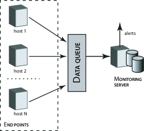
The processing is distributed. The data is collected by an agent program running on the end points. The data, aggregated over time frames for efficiency, is sent over the network to the data queue. The monitoring server consumes the data from the queue. Based on classification outcomes, the monitoring server may issue alerts when an anomalous event corresponding to one of the described scenarios is likely to take place.

There are a few tools [12, 13, 14] for collecting system calls in real time. Our solution uses sysdig [14]. Sysdig facilitates efficient recording of system calls in a high performance environment on modern Linux systems.

III-B Representation of Data

The main challenge in implementing the solution is bounding the amount of data collected and processed while preserving sufficient information for reliable classification. Using raw system call logs is infeasible:

• A single moderately loaded host can produce a million of system calls per second. Even for a single host the task would be challenging. Our architecture implies that data from many hosts is sent to the monitoring server for centralized processing.

• Raw system call logs have long temporal dependencies which are hard to learn: two system calls, one relying on the outcome of the other, can be hundreds of system calls apart.

• Although some previous research [3, 10] considered using system call arguments for constructing features for machine learning, we do not have a compact fixed-dimensional representation for system call arguments suitable for large-volume training and classification.

Consequently, we came up with a compact and easily learnable format based on sequences of system call count vectors:

• The data is a stream of vectors of integers, each vector is $\approx 300$ integers, one per system call type (there are $\approx 300$ system calls in Linux).

• Each vector corresponds to a fixed time interval $t$ (e.g. 1 second).

• Each vector component represents the number of calls issued during the time interval.

Let us consider an example. In this example we limit the monitoring to first 6 system calls:

1. exit

2. fork

3. read

4. write

5. open

6. close

Let us assume that process ‘foo’ performed the following sequence of system calls during a certain second:

    fork, open, read, write, read, write,
    read, write, read

The count vector representing the first second is:

exit	fork	read	write	open	close
0	1	3	2	1	0

Then, let us assume that during the next second we observe:

    write, read, write, close, exit

The corresponding count vector is

exit	fork	read	write	open	close
1	0	1	2	0	1

For input to machine learning model, the count vectors are normalized and combined into batches. The normalized two-second batch hence takes the following form:

sec	exit	fork	read	write	open	close
1	0.0	0.142	0.428	0.285	0.142	0.0
2	0.2	0.0	0.2	0.4	0.0	0.2

Vectors of counts of system calls are collected and sent for every monitored process at fixed short time intervals. However, the monitoring server processes sequences of system call vectors over longer time spans. This way, the performance guarantee is maintained through sending fixed amount of data per time unit independently of the activity on the host, but the temporal behavior is at least partially preserved. By varying the vector and sequence time durations, a balance between network and CPU load, on the one hand, and monitoring accuracy, on the other hand, can be adjusted depending on performance and accuracy requirements.

III-C Machine Learning Model

Figure 2: Machine learning model for classification of system call streams.

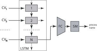
LSTM [15] (Long Short-Term Memory) deep learning architecture is particularly suitable for processing of sequences of system call count vectors. We use an LSTM network to train a model which reliably identifies processes by their count vector sequences and detects changes in their behavior.

The model structure is shown in Figure 2. The model is composed of a single-layer LSTM, followed by a fully-connected readout layer (FC), and a softmax layer (SM) for classification. Details about the machine learning model and algorithms are provided in Section IV.

III-D Main Results

We evaluated the solution on a laboratory setup and deployed the solution in the production environment. With 1-second count vectors and 10-seconds sequence length, the monitoring system achieves 90-93% accuracy for all scenarios. A single multi-core monitoring server is able to handle a network of 20,000 hosts. Empirical evaluation on the laboratory setup and the production environment are further described in Section V.

IV Machine Learning Architecture and Methodology

System calls are essentially sequential data and preserving the chronological information is important. Indeed, a sequence of system calls can be thought of as a sequence of words composing a sentence, the ordering of the words being critical to identify the meaning of the sentence. In order to preserve the temporal aspect of the system calls, we employ an LSTM-based architecture. LSTM is a type of recurrent neural network introduced in [15] that maps sequences of variable lengths to fixed dimensional vectors. It is particularly suitable for handling sequences of words or systems calls since the sequences can vary in length. LSTM is quite popular in the natural language community where it has been successfully applied to a vast variety of problems such as speech recognition or machine translation.

We now describe different variants of architectures that we experimented with. The architecture depicted in Figure 2 represents a neural network composed of a single-layer LSTM followed by a fully connected layer. The LSTM receives as input the sequence of count vectors in chronological order. We refer to this architecture as simple net.

Figure 3: Machine learning model based on bidirectional LSTM.

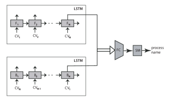
A slightly more complex architecture consists in two independent LSTMs where one receives the sequence in chronological order while the other receives it in reverse order (Figure 3). Such a network is called a bidirectional LSTM. This bidirectional LSTM outputs two fixed size vectors that are concatenated or averaged and fed to the following fully connected layer. We refer to this architecture as bidirectional net. A regular LSTM sees the sequence in chronological order and disregards the dependence that a later element in the sequence might have on one that precedes it. By allowing the network to look at the sequence in reverse order we take into account the dependence of the sequence in the other direction.

Finally, we experimented with an architecture that we called inception-like net inspired by the inception module introduced in [16]. Intuitively, considering a sequence at multiple scales at the same time, i.e. with multiple values of the time interval $t$, might give additional insights. If we take the example of a sentence, considering it as a sequence of words, but also as a sequence of couple of words might be useful to better understand the sentence. For an image, as discussed in [16], looking at an image with sliding windows at various scales helps making sense of features at different scales. Following this idea, the inception-like net consists in multiple LSTMs with tied-weights where each of them takes as input the same sequence but with different values of the time interval $t$. The different copies of the LSTM output fixed size vectors that are concatenated and fed to a fully connected layer.

The simple net performance is at par or slightly worse than with the more complex bidirectional net and inception-like net. Since the increase in performance is not significant, we opted for the simplest network. However, for the sake of completeness, results of the different architectures are reported in the next section.

V Empirical Evaluation

We evaluated our methodology in a laboratory setup as well as in production environment.

V-A Laboratory Setup

For the laboratory setup, we created a data collecting framework as shown in Figure 4.

Figure 4: Mail delivery client-server framework for evaluating the methodology

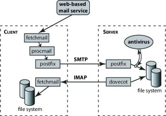
The setup consists of two hosts: the client and the server. A number of processes are involved in the workings of the setup. In the following description, the words in italic correspond to processes or process groups. The hosts collect emails from an external server. On the client, fetchmail is used to retrieve emails from a web-based email provider via the IMAP protocol. Then, procmail dispatches received emails, which are then sent by postfix to the server via SMTP protocol. The server’s postfix process receives the emails, passes them through the amavis antivirus and stores in the local filesystem. The dovecot process serves emails via the IMAP protocol. The emails are retrieved by the client’s fetchmail, and stored in the filesystem.

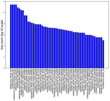
In addition to the mentioned processes or process groups, other utility processes run the hosts and are monitored. The setup is implemented as Docker [17] containers. In order to provide sufficient volume and diversity of the data processed, we opened a dedicated email account with a web-based email service, and subscribed the email account to many promotion and notification mailing lists, resulting in the average frequency of one incoming email per minute. For the empirical evaluation, we collected data from processes running both on the client and on the server during one week. The distribution of the count vectors lines is shown Figure 5

Figure 5: Histogram of count vector counts per process

For the empirical evaluation, we selected the 28 processes that are the most represented in our data and trained different models that aimed at classifying the processes based on their sequence of system calls. 80% of the data was used to train the classifiers and results were calculated on the 20% left out for testing. All the results reported for the LSTM-based architectures used LSTM with 64 hidden units and were trained using the Adam optimizer with an initial learning rate of $0.001$. The simple and bidirectional nets used a time interval $t=1$ while the inception-like net used $t=1,2,3$ simultaneously. L2 regularization was used on the parameters of the fully connected layer. Dropout on the input sequence didn’t seem to help significantly reduce overfitting in our experiments so results were omitted.

Results reported with Linear Support Vector Machine (SVM) [18], Logistic Regression [19], and Random Forest [20] were trained on a single time unit at a time, i.e. a one-dimensional vector representing $t$ seconds rather than a block of multiple time units (two-dimensional matrix). At test time, a process was classified using a majority vote over the multiple vectors representing it.

All the results reported are in terms of precision and recall per process (Table I). More precisely, the precisions and recalls over the different classes are averaged, this metric is known as macro-average precision and recall.

Model	Precision	Recall
Logistic Regression	0.843 (1e-16)	0.815 (1e-16)
Linear SVM	0.850 (1e-16)	0.827 (1e-16)
Random Forest	0.860 (0.006)	0.838 (9e-05)
Simple net	0.916 (0.01)	0.922 (0.003)
Bidirectional net	0.923 (0.01)	0.923 (0.003)
Inception-like net	0.924 (0.01)	0.925 (0.003)

TABLE I: Results for the laboratory setup. Results and standard deviations reported in parenthesis were obtained with 10 independent runs of the algorithms. A detailed description of the models is discussed in the main text.

V-B Production Environment

The results in the production environment (Table II) were obtained by training the model on data from one set of servers and evaluating the trained model on the data from a different set of servers, which makes the task more challenging. The servers may in general have different configurations, types and numbers of CPUs, and amounts of memory installed. Still, the model is able to generalize well on similar processes among different servers. The experiment was done on 20 different processes and the hyperparameters of the models were similar to the ones used for the laboratory setup.

Model	Precision	Recall
Logistic Regression	0.791 (1e-16)	0.741 (1e-16)
Linear SVM	0.792 (1e-16)	0.741 (1e-16)
Random Forest	0.850 (0.02)	0.795 (0.02)
Simple net	0.957 (0.03)	0.918 (0.03)
Bidirectional net	0.948 (0.04)	0.911 (0.04)
Inception-like net	0.965 (0.02)	0.931 (0.01)

TABLE II: Results for the production environment. Results and standard deviations reported in parenthesis were obtained with 10 independent runs of the algorithms. A detailed description of the models is discussed in the main text.

VI Summary and Future Work

The stream of system calls is a rich source of information about a computer system, but exact processing of the stream is impractical. Through a novel scheme which enables efficient processing of the stream while preserving properties essential for security and health monitoring, we are able to address several monitoring tasks at large scale with more than satisfactory accuracy. Future work is concerned with further advancing machine learning algorithms, as well as with moving from plain count vectors to a more compact but still as informative data representation.

References

- [1] S. Forrest, S. A. Hofmeyr, A. Somayaji, and T. A. Longstaff, “A sense of self for unix processes,” in Proceedings 1996 IEEE Symposium on Security and Privacy, May 1996, pp. 120–128.
- [2] C. Warrender, S. Forrest, and B. Pearlmutter, “Detecting intrusions using system calls: Alternative data models,” in IEEE symposium on security and privacy. IEEE Computer Society, 1999, pp. 133–145.
- [3] A. Liu, C. Martin, T. Hetherington, and S. Matzner, “A comparison of system call feature representations for insider threat detection,” in Information Assurance Workshop, 2005. IAW’05. Proceedings from the Sixth Annual IEEE SMC. IEEE, 2005, pp. 340–347.
- [4] C. Wressnegger, G. Schwenk, D. Arp, and K. Rieck, “A close look on n-grams in intrusion detection: Anomaly detection vs. classification,” in Proceedings of the 2013 ACM Workshop on Artificial Intelligence and Security, ser. AISec ’13. New York, NY, USA: ACM, 2013, pp. 67–76.
- [5] D. Gao, M. K. Reiter, and D. Song, “Gray-box extraction of execution graphs for anomaly detection,” in Proceedings of the 11th ACM Conference on Computer and Communications Security, ser. CCS ’04. New York, NY, USA: ACM, 2004, pp. 318–329.
- [6] D. Mutz, F. Valeur, G. Vigna, and C. Kruegel, “Anomalous system call detection,” ACM Trans. Inf. Syst. Secur., vol. 9, no. 1, pp. 61–93, Feb. 2006.
- [7] J. Xu and C. R. Shelton, “Intrusion detection using continuous time bayesian networks,” Journal of Artificial Intelligence Research, vol. 39, pp. 745–774, 2010.
- [8] G. Kim, H. Yi, J. Lee, Y. Paek, and S. Yoon, “Lstm-based system-call language modeling and robust ensemble method for designing host-based intrusion detection systems,” arXiv preprint arXiv:1611.01726, 2016.
- [9] K. Poulose Jacob and M. V. Surekha, “Anomaly detection using system call sequence sets.” Journal of Software, vol. 2, no. 6, 2007.
- [10] G. Tandon and P. K. Chan, “On the learning of system call attributes for host-based anomaly detection,” International Journal on Artificial Intelligence Tools, vol. 15, no. 06, pp. 875–892, 2006.
- [11] R. Canzanese, S. Mancoridis, and M. Kam, “System call-based detection of malicious processes,” in IEEE International Conference on Software Quality, Reliability and Security, ser. QRS ’15, 2015, pp. 119–124.
- [12] P. Kranenburg, B. Lankester, R. Sladkey, and D. Levin, “strace,” http://strace.io/, 1991–2017.
- [13] Sun Microsystems, “Dtrace,” http://dtrace.org/, 2005–2016.
- [14] Draios, Inc., “Sysdig,” http://sysdig.com/, 2012–2016.
- [15] S. Hochreiter and J. Schmidhuber, “Long short-term memory,” Neural Comput., vol. 9, no. 8, pp. 1735–1780, Nov. 1997.
- [16] C. Szegedy, W. Liu, Y. Jia, P. Sermanet, S. Reed, D. Anguelov, D. Erhan, V. Vanhoucke, and A. Rabinovich, “Going deeper with convolutions,” in Proceedings of the IEEE conference on computer vision and pattern recognition, 2015, pp. 1–9.
- [17] S. Hykes, “Docker,” http://docker.com/, 2013–2017.
- [18] R.-E. Fan, K.-W. Chang, C.-J. Hsieh, X.-R. Wang, and C.-J. Lin, “Liblinear: A library for large linear classification,” Journal of machine learning research, vol. 9, no. Aug, pp. 1871–1874, 2008.
- [19] S. H. Walker and D. B. Duncan, “Estimation of the probability of an event as a function of several independent variables,” Biometrika, vol. 54, no. 1-2, pp. 167–179, 1967.
- [20] L. Breiman, “Random forests,” Machine learning, vol. 45, no. 1, pp. 5–32, 2001.