Smooth and global Ising universal scaling functions

Abstract

We describe a method for approximating the universal scaling functions for the Ising model in a field. By making use of parametric coordinates, the free energy scaling function has a polynomial series everywhere. Its form is taken to be a sum of the simplest functions that contain the singularities which must be present: the Langer essential singularity and the Yang–Lee edge singularity. Requiring that the function match series expansions in the low- and high-temperature zero-field limits fixes the parametric coordinate transformation. For the two-dimensional Ising model, we show that this procedure converges exponentially with the order to which the series are matched, up to seven digits of accuracy. To facilitate use, we provide Python and Mathematica implementations of the code at both lowest order (three digit) and high accuracy.

I Introduction

At continuous phase transitions the thermodynamic properties of physical systems have singularities. Celebrated renormalization group analyses imply that not only the principal divergence but entire functions are universal, meaning that they will appear at any critical points that connect phases of the same symmetries in the same spatial dimension. The study of these universal functions is therefore doubly fruitful: it provides both a description of the physical or model system at hand, and every other system whose symmetries, interaction range, and dimension puts it in the same universality class.

The continuous phase transition in the two-dimensional Ising model is the most well studied, and its universal thermodynamic functions have likewise received the most attention. Without a field, an exact solution is known for some lattice models [1]. Precision numeric work both on lattice models and on the “Ising” conformal field theory (related by universality) have yielded high-order polynomial expansions of those functions, along with a comprehensive understanding of their analytic properties [2, 3, 4]. In parallel, smooth approximations of the Ising equation of state produce convenient, evaluable, differentiable empirical functions [5]. Despite being differentiable, these approximations become increasingly poor when derivatives are taken due to the neglect of subtle singularities.

This paper attempts to find the best of both worlds: a smooth approximate universal thermodynamic function that respects the global analytic properties of the Ising free energy. By constructing approximate functions with the correct singularities, corrections converge exponentially to the true function. To make the construction, we review the analytic properties of the Ising scaling function. Parametric coordinates are introduced that remove unnecessary singularities that are a remnant of the coordinate choice. The singularities known to be present in the scaling function are incorporated in their simplest form. Then, the arbitrary analytic functions that compose those coordinates are approximated by truncated polynomials whose coefficients are fixed by matching the series expansions of the universal function.

For the two-dimensional Ising model, this method produces scaling functions accurate to within $3\times 10^{-4}$ using just the values of the first three derivatives of the function evaluated at two points, e.g., critical amplitudes of the magnetization, susceptibility, and first generalized susceptibility. With six derivatives, it is accurate to about $10^{-7}$. We hope that with some refinement, this idea might be used to establish accurate scaling functions for critical behavior in other universality classes, doing for scaling functions what advances in conformal bootstrap did for critical exponents [6]. Mathematica and Python implementations will be provided in the supplemental material.

II Universal scaling functions

A renormalization group analysis predicts that certain thermodynamic functions will be universal in the vicinity of any critical point in the Ising universality class, from perturbed conformal fields to the end of the liquid–gas coexistence line. Here we will review precisely what is meant by universal.

Suppose one controls a temperature-like parameter $T$ and a magnetic field-like parameter $H$, which in the proximity of a critical point at $T=T_{c}$ and $H=0$ have normalized reduced forms $t=(T-T_{c})/T_{c}$ and $h=H/T$. Thermodynamic functions are derived from the free energy per site $f=(F-F_{c})/N$, which depends on $t$, $h$, and a litany of irrelevant parameters we will henceforth neglect. Explicit renormalization with techniques like the $\epsilon$-expansion or exact solutions like Onsager’s can be used calculated the flow of these parameters under continuous changes of scale $e^{\ell}$, yielding equations of the form

$$\frac{dt}{d\ell}=\frac{1}{\nu}t+\cdots \frac{dh}{d\ell}=\frac{\beta\delta}{\nu}h+\cdots \frac{df}{d\ell}=Df+\cdots$$ (1)

where $D=2$ is the dimension of space and $\nu=1$, $\beta=\frac{1}{8}$, and $\delta=15$ are dimensionless constants. The combination $\Delta=\beta\delta=\frac{15}{8}$ will appear often. The flow equations are truncated here, but in general all terms allowed by the symmetries of the parameters are present on their righthand side. By making a near-identity transformation to the coordinates and the free energy of the form $u_{t}(t,h)=t+\cdots$, $u_{h}(t,h)=h+\cdots$, and $u_{f}(f,u_{t},u_{h})\propto f(t,h)-f_{a}(t,h)$, one can bring the flow equations into the agreed upon simplest normal form

$$\frac{du_{t}}{d\ell}=\frac{1}{\nu}u_{t} \frac{du_{h}}{d\ell}=\frac{\Delta}{\nu}u_{h} \frac{du_{f}}{d\ell}=Du_{f}-\frac{1}{4\pi}u_{t}^{2}$$ (2)

which are exact as written [7]. The flow of the scaling fields $u_{t}$ and $u_{h}$ is made exactly linear, while that of the free energy is linearized as nearly as possible. The quadratic term in that equation is unremovable due to a ‘resonance’ between the value of $\nu$ and the spatial dimension in two dimensions, while its coefficient is chosen as a matter of convention, fixing the scale of $u_{t}$. Here the free energy $f=u_{f}+f_{a}$, where $u_{f}(u_{t},u_{h})$ is known as the singular part of the free energy, and $f_{a}(t,h)$ is a non-universal but analytic background free energy.

Solving these equations for $u_{f}$ yields

$$u_{f}(u_{t},u_{h}) =|u_{t}|^{D\nu}\mathcal{F}_{\pm}(u_{h}|u_{t}|^{-\Delta})+\frac{|u_{t}|^{D\nu}}{8\pi}\log u_{t}^{2}$$ (3)

$$=|u_{h}|^{D\nu/\Delta}\mathcal{F}_{0}(u_{t}|u_{h}|^{-1/\Delta})+\frac{|u_{t}|^{D\nu}}{8\pi}\log u_{h}^{2/\Delta}$$

where $\mathcal{F}_{\pm}$ and $\mathcal{F}_{0}$ are undetermined universal scaling functions related by a change of coordinates . The scaling functions are universal in the sense that any system in the same universality class will share the free energy (2), for suitable analytic functions $u_{t}$, $u_{h}$, and analytic background $f_{a}$ – the singular behavior is universal up to an analytic coordinate change. The invariant scaling combinations that appear as the arguments to the universal scaling functions will come up often, and we will use $\xi=u_{h}|u_{t}|^{-\Delta}$ and $\eta=u_{t}|u_{h}|^{-1/\Delta}$.

The analyticity of the free energy at places away from the critical point implies that the functions $\mathcal{F}_{\pm}$ and $\mathcal{F}_{0}$ have power-law expansions of their arguments about zero, the result of so-called Griffiths analyticity [9]. For instance, when $u_{t}$ goes to zero for nonzero $u_{h}$ there is no phase transition, and the free energy must be an analytic function of its arguments. It follows that $\mathcal{F}_{0}$ is analytic about zero. This is not the case at infinity: since

$$\mathcal{F}_{\pm}(\xi)=\xi^{D\nu/\Delta}\mathcal{F}_{0}(\pm\xi^{-1/\Delta})+\frac{1}{8\pi}\log\xi^{2/\Delta}$$ (4)

and $\mathcal{F}_{0}$ has a power-law expansion about zero, $\mathcal{F}_{\pm}$ has a series like $\xi^{D\nu/\Delta-j/\Delta}$ for $j\in\mathbb{N}$ at large $\xi$, along with logarithms. The nonanalyticity of these functions at infinite argument can be understood as an artifact of the chosen coordinates.

For the scale of $u_{t}$ and $u_{h}$, we adopt the same convention as used by [2]. The dependence of the nonlinear scaling variables on the parameters $t$ and $h$ is system-dependent, and their form can be found for common model systems (the square- and triangular-lattice Ising models) in the literature [4, 10].

III Singularities

III.1 Essential singularity at the abrupt transition

In the low temperature phase, the free energy has an essential singularity at zero field, which becomes a branch cut along the negative-$h$ axis when analytically continued to negative $h$ [11]. The origin can be schematically understood to arise from a singularity that exists in the imaginary free energy of the metastable phase of the model. When the equilibrium Ising model with positive magnetization is subjected to a small negative magnetic field, its equilibrium state instantly becomes one with a negative magnetization. However, under physical dynamics it takes time to arrive at this state, which happens after a fluctuation containing a sufficiently large equilibrium ‘bubble’ occurs.

The bulk of such a bubble of radius $R$ lowers the free energy by $2M|H|\pi R^{2}$, where $M$ is the magnetization, but its surface raises the free energy by $2\pi R\sigma$, where $\sigma$ is the surface tension between the stable–metastable interface. The bubble is sufficiently large to catalyze the decay of the metastable state when the differential bulk savings outweigh the surface costs. This critical bubble occurs with free energy cost

$$\Delta F_{c}\simeq\frac{\pi\sigma^{2}}{2M|H|}\simeq T\left(\frac{2M_{0}}{\pi\sigma_{0}^{2}}|\xi|\right)^{-1}$$ (5)

where $\sigma_{0}=\lim_{t\to 0}t^{-\mu}\sigma$ and $M_{0}=\lim_{t\to 0}t^{-\beta}M$ are the critical amplitudes for the surface tension and magnetization at zero field in the low-temperature phase [12]. In the context of statistical mechanics, Langer demonstrated that the decay rate is asymptotically proportional to the imaginary part of the free energy in the metastable phase, with

$$\operatorname{Im}F\propto\Gamma\sim e^{-\beta\Delta F_{c}}\simeq e^{-1/b|\xi|}$$ (6)

which can be more rigorously derived in the context of quantum field theory [13]. The constant $b=2M_{0}/\pi\sigma_{0}^{2}$ is predicted by known properties, e.g., for the square lattice $M_{0}$ and $\sigma_{0}$ are both predicted by Onsager’s solution [1], but for our conventions for $u_{t}$ and $u_{h}$, $M_{0}/\sigma_{0}^{2}=\bar{s}=2^{1/12}e^{-1/8}A^{3/2}$, where $A$ is Glaisher’s constant [2].

Figure 1: Analytic structure of the low-temperature scaling function $\mathcal{F}_{-}$ in the complex $\xi=u_{h}|u_{t}|^{-\Delta}\propto H$ plane. The circle depicts the essential singularity at the first order transition, while the solid line depicts Langer’s branch cut.

To lowest order, this singularity is a function of the scaling invariant $\xi$ alone. This suggests that it should be considered a part of the singular free energy, and thus part of the scaling function that composes it. There is substantial numeric evidence for this as well [14, 2]. We will therefore make the ansatz that

$$\operatorname{Im}\mathcal{F}_{-}(\xi+i0)=A_{0}\Theta(-\xi)\xi e^{-1/b|\xi|}\left[1+O(\xi)\right]$$ (7)

The linear prefactor can be found through a more careful accounting of the entropy of long-wavelength fluctuations in the droplet surface [15, 16]. In the Ising conformal field theory, the prefactor is known to be $A_{0}=\bar{s}/2\pi$ [13, 2]. The signature of this singularity in the scaling function is a superexponential divergence in the series coefficients about $\xi=0$, which asymptotically take the form

$$\mathcal{F}_{-}^{\infty}(m)=\frac{A_{0}}{\pi}b^{m-1}\Gamma(m-1)$$ (8)

III.2 Yang–Lee edge singularity

At finite size, the Ising model free energy is an analytic function of temperature and field because it is the logarithm of a sum of positive analytic functions. However, it can and does have singularities in the complex plane due to zeros of the partition function at complex argument, and in particular at imaginary values of field, $h$. Yang and Lee showed that in the thermodynamic limit of the high temperature phase of the model, these zeros form a branch cut along the imaginary $h$ axis that extends to $\pm i\infty$ starting at the point $\pm ih_{\mathrm{YL}}$ [17, 18]. The singularity of the phase transition occurs because these branch cuts descend and touch the real axis as $T$ approaches $T_{c}$, with $h_{\mathrm{YL}}\propto t^{\Delta}$. This implies that the high-temperature scaling function for the Ising model should have complex branch cuts beginning at $\pm i\xi_{\mathrm{YL}}$ for a universal constant $\xi_{\mathrm{YL}}$.

Figure 2: Analytic structure of the high-temperature scaling function $\mathcal{F}_{+}$ in the complex $\xi=u_{h}|u_{t}|^{-\Delta}\propto H$ plane. The squares depict the Yang–Lee edge singularities, while the solid lines depict branch cuts.

The Yang–Lee singularities, although only accessible with complex fields, are critical points in their own right, with their own universality class different from that of the Ising model [19]. Asymptotically close to this point, the scaling function $\mathcal{F}_{+}$ takes the form

$$\mathcal{F}_{+}(\xi)=A(\xi)+B(\xi)[1+(\xi/\xi_{\mathrm{YL}})^{2}]^{1+\sigma}+\cdots$$ (9)

with edge exponent $\sigma=-\frac{1}{6}$ and $A$ and $B$ analytic functions at $\xi_{\mathrm{YL}}$ [20, 2]. This creates a branch cut stemming from the critical point along the imaginary-$\xi$ axis with a growing imaginary part

$$\operatorname{Im}\mathcal{F}_{+}(i\xi\pm 0)=\pm\tilde{A}_{\mathrm{YL}}\Theta(\xi-\xi_{\mathrm{YL}})(\xi-\xi_{\mathrm{YL}})^{1+\sigma}[1+O[(\xi-\xi_{\mathrm{YL}})^{2}]]$$ (10)

This results in analytic structure for $\mathcal{F}_{+}$ shown in Fig. 2. The signature of this in the scaling function is an asymptotic behavior of the coefficients which goes like

$$\mathcal{F}_{+}^{\infty}(m)=A_{\mathrm{YL}}2(-1)^{2m}\theta_{\mathrm{YL}}^{1-\sigma-m}\binom{1-\sigma}{m}$$ (11)

IV Parametric coordinates

The invariant combinations $\xi=u_{h}|u_{t}|^{-\Delta}$ or $\eta=u_{t}|u_{h}|^{-1/\Delta}$ are natural variables to describe the scaling functions, but prove unwieldy when attempting to make smooth approximations. This is because, when defined in terms of these variables, scaling functions that have polynomial expansions at small argument have nonpolynomial expansions at large argument. Rather than deal with the creative challenge of dreaming up functions with different asymptotic expansions in different limits, we adopt another coordinate system, in terms of which a scaling function can be defined that has polynomial expansions in all limits.

The Schofield coordinates $R$ and $\theta$ are implicitly defined by

$$u_{t}(R,\theta)=R(1-\theta^{2}) u_{h}(R,\theta)=R^{\Delta}g(\theta)$$ (12)

where $g$ is an odd function whose first zero lies at $\theta_{0}>1$ [21]. We take

$$g(\theta)=\left(1-\frac{\theta^{2}}{\theta_{0}^{2}}\right)\sum_{i=0}^{\infty}g_{i}\theta^{2i+1}.$$ (13)

This means that $\theta=0$ corresponds to the high-temperature zero-field line, $\theta=1$ to the critical isotherm at nonzero field, and $\theta=\theta_{0}$ to the low-temperature zero-field (phase coexistence) line. In practice the infinite series in (13) cannot be entirely fixed, and it will be truncated at finite order.

Figure 3: Example of the parametric coordinates. Solid lines are of constant $R=\frac{1}{2},1,\ldots,8\frac{1}{2}$ and dashed lines are of constant $\theta=\pm 0\theta_{0},\frac{1}{16}\theta_{0},\ldots,\theta_{0}$ for $g(\theta)$ taken from the $n=6$ entry of Table 2.

One can now see the convenience of these coordinates. Both invariant scaling combinations depend only on $\theta$, as

$$\xi=u_{h}|u_{t}|^{-\Delta}=\frac{g(\theta)}{|1-\theta^{2}|^{\Delta}} \eta=u_{t}|u_{h}|^{-1/\Delta}=\frac{1-\theta^{2}}{|g(\theta)|^{1/\Delta}}$$ (14)

Moreover, both scaling variables have polynomial expansions in $\theta$ near zero, with

$$\xi=g^{\prime}(0)\theta+\cdots \theta\simeq 0$$ for (15)

$$\xi=g^{\prime}(\theta_{0})(\theta_{0}^{2}-1)^{-\Delta}(\theta-\theta_{0})+\cdots \theta\simeq\theta_{0}$$ for (16)

$$\eta=-2(\theta-1)g(1)^{-1/\Delta}+\cdots \text{for $\theta\simeq 1$}.$$ (17)

Since the scaling functions $\mathcal{F}_{\pm}(\xi)$ and $\mathcal{F}_{0}(\eta)$ have polynomial expansions about small $\xi$ and $\eta$, respectively, this implies both will have polynomial expansions in $\theta$ everywhere.

Therefore, in Schofield coordinates one expects to be able to define a global scaling function $\mathcal{F}(\theta)$ which has a polynomial expansion in its argument for all real $\theta$ by

$$u_{f}(R,\theta)=R^{D\nu}\mathcal{F}(\theta)+(1-\theta^{2})^{2}\frac{R^{2}}{8\pi}\log R^{2}$$ (18)

For small $\theta$, $\mathcal{F}(\theta)$ will resemble $\mathcal{F}_{+}$, for $\theta$ near one it will resemble $\mathcal{F}_{0}$, and for $\theta$ near $\theta_{0}$ it will resemble $\mathcal{F}_{-}$. This can be seen explicitly using the definitions (12) to relate the above form to the original scaling functions, giving

$$\mathcal{F}(\theta) =|1-\theta^{2}|^{D\nu}\mathcal{F}_{\pm}\left[g(\theta)|1-\theta^{2}|^{-\Delta}\right]+\frac{(1-\theta^{2})^{2}}{8\pi}\log(1-\theta^{2})^{2}$$ (19)

$$=|g(\theta)|^{D\nu/\Delta}\mathcal{F}_{0}\left[(1-\theta^{2})|g(\theta)|^{-1/\Delta}\right]+\frac{(1-\theta^{2})^{2}}{8\pi}\log g(\theta)^{2/\Delta}$$

This leads us to expect that the singularities present in these functions will likewise be present in $\mathcal{F}(\theta)$. The analytic structure of this function is shown in Fig. 4. Two copies of the Langer branch cut stretch out from $\pm\theta_{0}$, where the equilibrium phase ends, and the Yang–Lee edge singularities are present on the imaginary-$\theta$ line (because $\mathcal{F}$ has the same symmetry in $\theta$ as $\mathcal{F}_{+}$ has in $\xi$).

The location of the Yang–Lee edge singularities can be calculated directly from the coordinate transformation (12). Since $g(\theta)$ is an odd real polynomial for real $\theta$, it is imaginary for imaginary $\theta$. Therefore,

$$i\xi_{\mathrm{YL}}=\frac{g(i\theta_{\mathrm{YL}})}{(1+\theta_{\mathrm{YL}}^{2})^{-\Delta}}$$ (20)

The location $\theta_{0}$ is not fixed by any principle.

Figure 4: Analytic structure of the global scaling function $\mathcal{F}$ in the complex $\theta$ plane. The circles depict essential singularities of the first order transitions, the squares the Yang–Lee singularities, and the solid lines depict branch cuts.

V Functional form for the parametric free energy

As we have seen in the previous sections, the unavoidable singularities in the scaling functions are readily expressed as singular functions in the imaginary part of the free energy.

Our strategy follows. First, we take the singular imaginary parts of the scaling functions $\mathcal{F}_{\pm}(\xi)$ and truncate them to the lowest order accessible under polynomial coordinate changes of $\xi$. Then, we constrain the imaginary part of $\mathcal{F}(\theta)$ to have this simplest form, implicitly defining the analytic parametric coordinate change $g(\theta)$. Third, we perform a Kramers–Kronig type transformation to establish an explicit form for the real part of $\mathcal{F}(\theta)$ involving a second analytic function $G(\theta)$. Finally, we make good on the constraint made in the second step by fitting the coefficients of $g(\theta)$ and $G(\theta)$ to reproduce the correct known series coefficients of $\mathcal{F}_{\pm}$.

This success of this stems from the commutative diagram below. So long as the application of Schofield coordinates and the Kramers–Kronig relation can be said to commute, we may assume we have found correct coordinates for the simplest form of the imaginary part to be fixed later by the real part.

We require that, for $\theta\in\mathbb{R}$

$$\operatorname{Im}\mathcal{F}(\theta+0i)=\operatorname{Im}\mathcal{F}_{0}(\theta+0i)=C_{0}[\Theta(\theta-\theta_{0})\mathcal{I}(\theta)-\Theta(-\theta-\theta_{0})\mathcal{I}(-\theta)]$$ (21)

where

$$\mathcal{I}(\theta)=(\theta-\theta_{0})e^{-1/B(\theta-\theta_{0})}$$ (22)

reproduces the essential singularity in (7). Independently, we require for $\theta\in\mathbb{R}$

$$\operatorname{Im}\mathcal{F}(i\theta+0)=\operatorname{Im}\mathcal{F}_{\mathrm{YL}}(i\theta+0)=\frac{1}{2}C_{\mathrm{YL}}\left[\Theta(\theta-\theta_{\mathrm{YL}})(\theta-\theta_{\mathrm{YL}})^{1+\sigma}-\Theta(\theta+\theta_{\mathrm{YL}})(\theta+\theta_{\mathrm{YL}})^{1+\sigma}\right]$$ (23)

Fixing these requirements for the imaginary part of $\mathcal{F}(\theta)$ fixes its real part up to an analytic even function $G(\theta)$, real for real $\theta$.

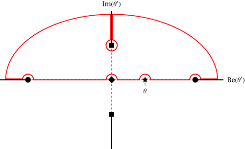
Figure 5: Integration contour over the global scaling function $\mathcal{F}$ in the complex $\theta$ plane used to produce the dispersion relation. The circular arc is taken to infinity, while the circles around the singularities are taken to zero.

To find the real part of the nonanalytic part of the scaling function, we make use of the identity

$$0=\oint_{\mathcal{C}}d\vartheta\,\frac{\mathcal{F}(\vartheta)}{\vartheta^{2}(\vartheta-\theta)}$$ (24)

where $\mathcal{C}$ is the contour in Figure 5. The integral is zero because there are no singularities enclosed by the contour. The only nonvanishing contributions from this contour as the radius of the semicircle is taken to infinity are along the real line and along the branch cut in the upper half plane. For the latter contributions, the real parts of the integration up and down cancel out, while the imaginary part doubles. This gives

$$0 =\left[\int_{-\infty}^{\infty}+\lim_{\epsilon\to 0}\left(\int_{i\infty-\epsilon}^{i\theta_{\mathrm{YL}}-\epsilon}+\int^{i\infty+\epsilon}_{i\theta_{\mathrm{YL}}+\epsilon}\right)\right]d\vartheta\,\frac{\mathcal{F}(\vartheta)}{\vartheta^{2}(\vartheta-\theta)}$$ (25)

$$=\int_{-\infty}^{\infty}d\vartheta\,\frac{\mathcal{F}(\vartheta)}{\vartheta^{2}(\vartheta-\theta)}+2i\int_{i\theta_{\mathrm{YL}}}^{i\infty}d\theta^{\prime}\,\frac{\operatorname{Im}\mathcal{F}(\vartheta)}{\vartheta^{2}(\vartheta-\theta)}$$

$$=-i\pi\frac{\mathcal{F}(\theta)}{\theta^{2}}+\mathcal{P}\int_{-\infty}^{\infty}d\vartheta\,\frac{\mathcal{F}(\vartheta)}{\vartheta^{2}(\vartheta-\theta)}+2i\int_{i\theta_{\mathrm{YL}}}^{i\infty}d\vartheta\,\frac{\operatorname{Im}\mathcal{F}(\vartheta)}{\vartheta^{2}(\vartheta-\theta)}$$

where $\mathcal{P}$ is the principle value. In principle one would need to account for the residue of the pole at zero, but since its order is less than two and $\mathcal{F}(0)=\mathcal{F}^{\prime}(0)=0$, this evaluates to zero. Rearranging, this gives

$$\mathcal{F}(\theta)=\frac{\theta^{2}}{i\pi}\mathcal{P}\int_{-\infty}^{\infty}d\vartheta\,\frac{\mathcal{F}(\vartheta)}{\vartheta^{2}(\vartheta-\theta)}+\frac{2\theta^{2}}{\pi}\int_{i\theta_{\mathrm{YL}}}^{i\infty}d\vartheta\,\frac{\operatorname{Im}\mathcal{F}(\theta^{\prime})}{\vartheta^{2}(\vartheta-\theta)}$$ (26)

Taking the real part of both sides, we find

$$\operatorname{Re}\mathcal{F}(\theta)=\frac{\theta^{2}}{\pi}\mathcal{P}\int_{-\infty}^{\infty}d\vartheta\,\frac{\operatorname{Im}\mathcal{F}(\vartheta)}{\vartheta^{2}(\vartheta-\theta)}-\frac{2\theta^{2}}{\pi}\int_{\theta_{\mathrm{YL}}}^{\infty}d\vartheta\,\frac{\operatorname{Im}\mathcal{F}(i\vartheta)}{\vartheta(\vartheta^{2}+\theta^{2})}$$ (27)

Because the real part of $\mathcal{F}$ is even, the imaginary part must be odd. Therefore

$$\operatorname{Re}\mathcal{F}(\theta)=\frac{\theta^{2}}{\pi}\int_{\theta_{0}}^{\infty}d\vartheta\,\frac{\operatorname{Im}\mathcal{F}(\vartheta)}{\vartheta^{2}}\left(\frac{1}{\vartheta-\theta}+\frac{1}{\vartheta+\theta}\right)-\frac{2\theta^{2}}{\pi}\int_{\theta_{\mathrm{YL}}}^{\infty}d\vartheta\,\frac{\operatorname{Im}\mathcal{F}(i\vartheta)}{\vartheta(\vartheta^{2}+\theta^{2})}$$ (28)

Evaluating these ordinary integrals, we find for $\theta\in\mathbb{R}$

$$\operatorname{Re}\mathcal{F}(\theta)=\operatorname{Re}\mathcal{F}_{0}(\theta)+\mathcal{F}_{\mathrm{YL}}(\theta)+G(\theta)$$ (29)

where

$$\operatorname{Re}\mathcal{F}_{0}(\theta)=C_{0}[\mathcal{R}(\theta)+\mathcal{R}(-\theta)]$$ (30)

where $\mathcal{R}$ is given by the function

$$\mathcal{R}(\theta)=\frac{1}{\pi}\left[\theta_{0}e^{1/B\theta_{0}}\operatorname{Ei}(-1/B\theta_{0})+(\theta-\theta_{0})e^{-1/B(\theta-\theta_{0})}\operatorname{Ei}(1/B(\theta-\theta_{0}))\right]$$ (31)

and

$$\mathcal{F}_{\mathrm{YL}}(\theta)=2C_{\mathrm{YL}}\left[2(\theta^{2}+\theta_{\mathrm{YL}}^{2})^{(1+\sigma)/2}\cos\left((1+\sigma)\tan^{-1}\frac{\theta}{\theta_{\mathrm{YL}}}\right)-\theta_{\mathrm{YL}}^{1+\sigma}\right]$$ (32)

We have also included the analytic part $G$, which we assume has a simple series expansion

$$G(\theta)=\sum_{i=1}^{\infty}G_{i}\theta^{2i}$$ (33)

From the form of the real part, we can infer the form of $\mathcal{F}$ that is analytic for the whole complex plane except at the singularities and branch cuts previously discussed. For $\theta\in\mathbb{C}$, we take

$$\mathcal{F}(\theta)=\mathcal{F}_{0}(\theta)+\mathcal{F}_{\mathrm{YL}}(\theta)+G(\theta),$$ (34)

where

$$\mathcal{F}_{0}(\theta)=C_{0}\left\{\mathcal{R}(\theta)+\mathcal{R}(-\theta)+i\operatorname{sgn}(\operatorname{Im}\theta)[\mathcal{I}(\theta)-\mathcal{I}(-\theta)]\right\}$$ (35)

VI Fitting

The scaling function has a number of free parameters: the position $\theta_{0}$ of the abrupt transition, prefactors in front of singular functions from the abrupt transition and the Yang–Lee point, the coefficients in the analytic part $G$ of the scaling function, and the coefficients in the undetermined coordinate function $g$.

The other parameters $B$, $C_{0}$, $\theta_{YL}$, and $C_{YL}$ are determined or further constrained by known properties. For $\theta>\theta_{0}$, the form (7) can be expanded around $\theta=\theta_{0}$ to yield

$$\operatorname{Im}u_{f} \simeq A_{0}u_{t}(\theta)^{D\nu}\xi(\theta)\exp\left\{\frac{1}{b\xi(\theta)}\right\}$$ (36)

$$=A_{0}R^{D\nu}(\theta_{0}^{2}-1)^{D\nu}\xi^{\prime}(\theta_{0})(\theta-\theta_{0})\exp\left\{\frac{1}{b\xi^{\prime}(\theta_{0})}\left(\frac{1}{\theta-\theta_{0}}-\frac{\xi^{\prime\prime}(\theta_{0})}{2\xi^{\prime}(\theta_{0})}\right)\right\}\left(1+O[(\theta-\theta_{0})^{2}]\right)$$

Comparing this with the requirement (21), we find that

$$B=-b\xi^{\prime}(\theta_{0})=-b\frac{g^{\prime}(\theta_{0})}{(\theta_{0}^{2}-1)^{1/\Delta}}$$ (37)

and

$$C_{0} =A_{0}t(\theta_{0}^{2}-1)^{D\nu}\xi^{\prime}(\theta_{0})\exp\left\{-\frac{\xi^{\prime\prime}(\theta_{0})}{2b\xi^{\prime}(\theta_{0})^{2}}\right\}$$ (38)

$$=A_{0}(\theta_{0}^{2}-1)^{D\nu-\Delta}g^{\prime}(\theta_{0})\exp\left\{-\frac{1}{b}\left(\frac{(\theta_{0}^{2}-1)^{\Delta}g^{\prime\prime}(\theta_{0})}{2g^{\prime}(\theta_{0})^{2}}-\frac{2\Delta(\theta_{0}^{2}-1)^{\Delta-1}\theta_{0}}{g^{\prime}(\theta_{0})}\right)\right\}$$

fixing $B$ and $C_{0}$. Similarly, (20) puts a constraint on the value of $\theta_{\mathrm{YL}}$, while the known amplitude of the Yang–Lee branch cut fixes the value of $C_{\mathrm{YL}}$ by

$$u_{f} \simeq A_{\mathrm{YL}}|u_{h}(\theta)|^{D\nu/\Delta}(\eta_{\mathrm{Y}L}-\eta(\theta))^{1+\sigma}$$ (39)

$$=A_{\mathrm{YL}}R^{D\nu}|g(i\theta_{\mathrm{YL}})|^{D\nu/\Delta}[-\eta^{\prime}(i\theta_{\mathrm{YL}})]^{1+\sigma}(\theta-i\theta_{\mathrm{YL}})^{1+\sigma}\left(1+O[(\theta-i\theta_{\mathrm{YL}})^{2}]\right)$$

$$\simeq R^{D\nu}\mathcal{F}_{\mathrm{YL}}(\theta)=C_{\mathrm{YL}}R^{D\nu}(\theta-i\theta_{\mathrm{YL}})^{1+\sigma}\left(1+O[(\theta-i\theta_{\mathrm{YL}})^{2}]\right)$$

$$C_{\mathrm{YL}}=A_{\mathrm{YL}}|g(i\theta_{\mathrm{YL}})|^{D\nu/\Delta}\left[\frac{-\eta^{\prime}(i\theta_{\mathrm{YL}})}{2i\theta_{\mathrm{YL}}}\right]^{1+\sigma}$$ (40)

where $A_{\mathrm{YL}}=-1.37(2)$ and $\xi_{\mathrm{YL}}=0.18930(5)$ [2]. Because these parameters are not known exactly, these constraints are added to the weighted sum of squares rather than substituted in.

This leaves as unknown variables the positions $\theta_{0}$ and $\theta_{\mathrm{YL}}$ of the abrupt transition and Yang–Lee edge singularity, the amplitude $C_{\mathrm{YL}}$ of the latter, and the unknown functions $G$ and $g$. We determine these approximately by iteration in the polynomial order at which the free energy and its derivative matches known results, shown in Table 1. We write as a cost function the difference between the known series coefficients of the scaling functions $\mathcal{F}_{\pm}$ and the series coefficients of our parametric form evaluated at the same points, $\theta=0$ and $\theta=\theta_{0}$, weighted by the uncertainty in the value of the known coefficients or by a machine-precision cutoff, whichever is larger. We also add the difference between the predictions for $A_{\mathrm{YL}}$ and $\xi_{\mathrm{YL}}$ and their known numeric values, again weighted by their uncertainty. In order to encourage convergence, we also add weak residuals $j!g_{j}$ and $j!G_{j}$ encouraging the coefficients of the analytic functions $g$ and $G$ in (13) and (33) to stay small. This can be interpreted as a prior which expects these functions to be analytic, and therefore have series coefficients which decay with a factorial.

A Levenberg–Marquardt algorithm is performed on the cost function to find a parameter combination which minimizes it. As larger polynomial order in the series are fit, the truncations of $G$ and $g$ are extended to higher order so that the codimension of the fit is constant. We performed this procedure starting at $n=2$ (matching the scaling function at the low and high temperature zero field points to quadratic order), up through $n=6$. At higher order we began to have difficulty minimizing the cost. The resulting fit coefficients can be found in Table 2.

Precise results exist for the value of the scaling function and its derivatives at the critical isotherm, or equivalently for the series coefficients of the scaling function $\mathcal{F}_{0}$. Since we do not use these coefficients in our fits, the error in the approximate scaling functions and their derivatives can be evaluated by comparison to their known values at the critical isotherm, or $\theta=1$. The difference between the numeric values of the coefficients $\mathcal{F}_{0}^{(m)}$ and those predicted by the iteratively fit scaling functions are shown in Fig. 6. For the values for which we were able to make a fit, the error in the function and its first several derivatives appear to trend exponentially towards zero in the polynomial order $n$. The predictions of our fits at the critical isotherm can be compared with the numeric values to higher order in Fig. 7, where the absolute values of both are plotted.

$m$	$\mathcal{F}_{-}^{(m)}$	$\mathcal{F}_{0}^{(m)}$	$\mathcal{F}_{+}^{(m)}$
0	0	$-1.197\,733\,383\,797\ldots$	0
1	$-1.357\,838\,341\,707\ldots$	$0.318\,810\,124\,891\ldots$	0
2	$-0.048\,953\,289\,720\ldots$	$0.110\,886\,196\,683(2)$	$-1.845\,228\,078\,233\ldots$
3	$0.038\,863\,932(3)$	$-0.016\,426\,894\,65(2)$	0
4	$-0.068\,362\,119(2)$	$-2.639\,978(1)\times 10^{-4}$	$8.333\,711\,750(5)$
5	$0.183\,883\,70(1)$	$5.140\,526(1)\times 10^{-4}$	0
6	$-0.659\,171\,4(1)$	$2.088\,65(1)\times 10^{-4}$	$-95.168\,96(1)$
7	$2.937\,665(3)$	$4.481\,9(1)\times 10^{-5}$	0
8	$-15.61(1)$	$3.16\times 10^{-7}$	1457.62(3)
9	96.76	$-4.31\times 10^{-6}$	0
10	$-679$	$-1.99\times 10^{-6}$	$-25\,891(2)$
11	$5.34\times 10^{3}$		0
12	$-4.66\times 10^{4}$		$5.02\times 10^{5}$
13	$4.46\times 10^{5}$		0
14	$-4.66\times 10^{6}$		$-1.04\times 10^{7}$

Table 1: Known series coefficients for the universal scaling functions. Those with trailing dots are known exactly or have closed integral representations. Those with listed uncertainties are taken from Mangazeev et al. [3]. Those without are taken from Fonseca et al., and are assumed to be accurate to within their last digit [2].

$n$	$\theta_{0}$	$\theta_{\mathrm{YL}}$	$C_{\mathrm{YL}}$	$G_{1}$	$G_{2}$	$G_{3}$	$G_{4}$
2	1.14841	0.989667	$-0.172824$	$-0.310183$	0.247454
3	1.25421	0.602056	$-0.385664$	$-0.352751$	0.258243
4	1.31649	0.640019	$-0.356397$	$-0.355055$	0.234659	$-0.00190837$
5	1.34032	0.623811	$-0.380029$	$-0.351275$	0.237046	$-0.00731973$
6	1.36261	0.646215	$-0.355764$	$-0.352058$	0.233166	$-0.00664903$	$-0.00168991$

$n$	$g_{0}$	$g_{1}$	$g_{2}$	$g_{3}$	$g_{4}$	$g_{5}$
2	0.373691	$-0.0216363$
3	0.448379	$-0.0220323$	0.000222006
4	0.441074	$-0.0348177$	0.000678173	$-0.0000430514$
5	0.443719	$-0.0460994$	$-0.000745834$	0.0000596688	$-0.00000440308$
6	0.438453	$-0.0531270$	$-0.00391478$	$-0.000408016$	0.0000262629	$-0.00000109745$

Table 2: Free parameters in the fit of the parametric coordinate transformation and scaling form to known values of the scaling function series coefficients for $\mathcal{F}_{\pm}$. The fit at stage $n$ matches those coefficients up to and including order $n$. Uncertainty estimates are difficult to quantify directly.

Figure 6: The error in the $m$th derivative of the scaling function $\mathcal{F}_{0}$ with respect to $\eta$ evaluated at $\eta=0$, as a function of the polynomial order $n$ at which the scaling function was fit. The point $\eta=0$ corresponds to the critical isotherm at $T=T_{c}$ and $H>0$, roughly midway between the two limits used in the fit, at $H=0$ and $T$ above and below $T_{c}$. Convergence here should reflect overall convergence of our scaling function at all $\theta$.

Figure 7: The series coefficients for the scaling function $\mathcal{F}_{0}$ as a function of polynomial order $m$. The numeric values are from Table 1 and are partially obscured by the other data.

Even at $n=2$, where only seven unknown parameters have been fit, the results are accurate to within $3\times 10^{-4}$. This approximation for the scaling functions also captures the singularities at the high- and low-temperature zero-field points well. A direct comparison between the magnitudes of the series coefficients known numerically and those given by the approximate functions is shown for $\mathcal{F}_{-}$ in Fig. 8, for $\mathcal{F}_{+}$ in Fig. 9, and for $\mathcal{F}_{0}$ in Fig. 7.

Figure 8: The series coefficients for the scaling function $\mathcal{F}_{-}$ as a function of polynomial order $m$. The numeric values are from Table 1, and those of Caselle et al. are from the most accurate scaling function listed in [5]. The deviation at high polynomial order illustrates the lack of the essential singularity in the form of Caselle et al..

Figure 9: The series coefficients for the scaling function $\mathcal{F}_{+}$ as a function of polynomial order $m$. The numeric values are from Table 1, and those of Caselle et al. are from the most accurate scaling function listed in [5]. Note all agree well for $H$ near zero, $T>T_{c}$, as does the function of Caselle et al.

Also shown are the ratio between the series in $\mathcal{F}_{-}$ and $\mathcal{F}_{+}$ and their asymptotic behavior, in Fig. 10 and Fig. 11, respectively. While our functions have the correct asymptotic behavior by construction, for $\mathcal{F}_{-}$ they appear to do poorly in an intermediate regime which begins at larger order as the order of the fit becomes larger. This is due to the analytic part of the scaling function and the analytic coordinate change, which despite having small high-order coefficients as functions of $\theta$ produce large intermediate derivatives as functions of $\xi$. We suspect that the nature of the truncation of these functions is responsible, and are investigating modifications that would converge better. Notice that this infelicity does not appear to cause significant errors in the function $\mathcal{F}_{-}(\theta)$ or its low order derivatives, as evidenced by the convergence in Fig. 6.

Figure 10: The series coefficients for the scaling function $\mathcal{F}_{-}$ as a function of polynomial order $m$, rescaled by their asymptotic limit $\mathcal{F}_{-}^{\infty}(m)$ from (8). The numeric values are from Table 1, and those of Caselle et al. are from the most accurate scaling function listed in [5]. Note that our $n=6$ fit generates significant deviations in polynomial coefficients $m$ above around 10.

Figure 11: The series coefficients for the scaling function $\mathcal{F}_{+}$ as a function of polynomial order $m$, rescaled by their asymptotic limit $\mathcal{F}_{+}^{\infty}(m)$ from (11). The numeric values are from Table 1, and those of Caselle et al. are from the most accurate scaling function listed in [5].

Besides reproducing the high derivatives in the series, the approximate functions defined here feature the appropriate singularity at the abrupt transition. Fig. 12 shows the ratio of subsequent series coefficients for $\mathcal{F}_{-}$ as a function of the inverse order, which should converge in the limit of $m\to 0$ to the inverse radius of convergence for the series. Approximations for the function without the explicit singularity have a nonzero radius of convergence, where both the numeric data and the approximate functions defined here show the appropriate divergence in the ratio.

Figure 12: Sequential ratios of the series coefficients of the scaling function $\mathcal{F}_{-}$ as a function of inverse polynomial order $m$. The extrapolated $y$-intercept of this plot gives the radius of convergence of the series, which should be zero due to the essential singularity (as seen in the known numeric values and in this work). Caselle et al. do not incorporate the essential singularity.

VII Outlook

We have introduced explicit approximate functions forms for the two-dimensional Ising universal scaling function in the relevant variables. These functions are smooth to all orders, include the correct singularities, and appear to converge exponentially to the function as they are fixed to larger polynomial order.

This method, although spectacularly successful, could be improved. It becomes difficult to fit the unknown functions at progressively higher order due to the complexity of the chain-rule derivatives, and we find an inflation of predicted coefficients in our higher-precision fits. These problems may be related to the precise form and method of truncation for the unknown functions.

The successful smooth description of the Ising free energy produced in part by analytically continuing the singular imaginary part of the metastable free energy inspires an extension of this work: a smooth function that captures the universal scaling through the coexistence line and into the metastable phase. The functions here are not appropriate for this except for a small distance into the metastable phase, at which point the coordinate transformation becomes untrustworthy. In order to do this, the parametric coordinates used here would need to be modified so as to have an appropriate limit as $\theta\to\infty$.

References

• Onsager [1944] L. Onsager, Crystal statistics. I. a two-dimensional model with an order-disorder transition, Physical Review 65, 117 (1944).
• Fonseca and Zamolodchikov [2003] P. Fonseca and A. Zamolodchikov, Ising field theory in a magnetic field: Analytic properties of the free energy, Journal of Statistical Physics 110, 527 (2003).
• Mangazeev et al. [2008] V. V. Mangazeev, M. T. Batchelor, V. V. Bazhanov, and M. Y. Dudalev, Variational approach to the scaling function of the 2d Ising model in a magnetic field, Journal of Physics A: Mathematical and Theoretical 42, 042005 (2008).
• Mangazeev et al. [2010] V. V. Mangazeev, M. Y. Dudalev, V. V. Bazhanov, and M. T. Batchelor, Scaling and universality in the two-dimensional Ising model with a magnetic field, Physical Review E 81, 060103 (2010).
• Caselle et al. [2001] M. Caselle, M. Hasenbusch, A. Pelissetto, and E. Vicari, The critical equation of state of the two-dimensional Ising model, Journal of Physics A: Mathematical and General 34, 2923 (2001).
• Gliozzi and Rago [2014] F. Gliozzi and A. Rago, Critical exponents of the 3d Ising and related models from conformal bootstrap, Journal of High Energy Physics 2014, 042 (2014).
• Raju et al. [2019] A. Raju, C. B. Clement, L. X. Hayden, J. P. Kent-Dobias, D. B. Liarte, D. Z. Rocklin, and J. P. Sethna, Normal form for renormalization groups, Physical Review X 9, 021014 (2019).
• Note [1] To connect the results of this paper with Mangazeev and Fonseca, one can write $\mathcal{F}_{0}(\eta)=\tilde{\Phi}(-\eta)=\Phi(-\eta)+(\eta^{2}/8\pi)\mathop{log}\nolimits\eta^{2}$ and $\mathcal{F}_{\pm}(\xi)=G_{\mathrm{high}/\mathrm{low}}(\xi)$.
• Griffiths [1967] R. B. Griffiths, Thermodynamic functions for fluids and ferromagnets near the critical point, Physical Review 158, 176 (1967).
• Clement [2019] C. Clement, Respect Your Data: Topics in Inference and Modeling in PhysicsPh.D. thesis, Cornell University, Ann Arbor (2019).
• Langer [1967] J. S. Langer, Theory of the condensation point, Annals of Physics 41, 108 (1967).
• Kent-Dobias [2020] J. P. Kent-Dobias, Novel Critical PhenomenaPh.D. thesis, Cornell University, Ann Arbor (2020).
• Voloshin [1985] M. B. Voloshin, Decay of false vacuum in ($1+1$) dimensions, Soviet Journal of Nuclear Physics 42, 644 (1985).
• Enting and Baxter [1980] I. G. Enting and R. J. Baxter, An investigation of the high-field series expansions for the square lattice Ising model, Journal of Physics A: Mathematical and General 13, 3723 (1980).
• Günther et al. [1980] N. J. Günther, D. J. Wallace, and D. A. Nicole, Goldstone modes in vacuum decay and first-order phase transitions, Journal of Physics A: Mathematical and General 13, 1755 (1980).
• Houghton and Lubensky [1980] A. Houghton and T. C. Lubensky, The metastable Ising magnet in a negative field, Physics Letters A 77, 479 (1980).
• Yang and Lee [1952] C. N. Yang and T. D. Lee, Statistical theory of equations of state and phase transitions. I: Theory of condensation, Physical Review 87, 404 (1952).
• Lee and Yang [1952] T. D. Lee and C. N. Yang, Statistical theory of equations of state and phase transitions. II: Lattice gas and Ising model, Physical Review 87, 410 (1952).
• Fisher [1978] M. E. Fisher, Yang-Lee edge singularity and $\phi^{3}$ field theory, Physical Review Letters 40, 1610 (1978).
• Cardy [1985] J. L. Cardy, Conformal invariance and the Yang-Lee edge singularity in two dimensions, Physical Review Letters 54, 1354 (1985).
• Schofield [1969] P. Schofield, Parametric representation of the equation of state near a critical point, Physical Review Letters 22, 606 (1969).