Lipschitz stability for an inverse hyperbolic problem of determining two coefficients by a finite number of observations

Abstract

We consider an inverse problem of reconstructing two spatially varying coefficients in an acoustic equation of hyperbolic type using interior data of solutions with suitable choices of initial condition. Using a Carleman estimate, we prove Lipschitz stability estimates which ensures unique reconstruction of both coefficients. Our theoretical results are justified by numerical studies on the reconstruction of two unknown coefficients using noisy backscattered data.

1 Statement of the problem

1.1 Introduction

The main purpose of this paper is to study the inverse problem of determining simultaneously the function $\rho(x)$ and the conductivity $p(x)$ in the following:

$$\rho(x)\partial_{t}^{2}u-\mathrm{div}\,(p(x)\nabla u)=0$$ (1.1)

from a finite number of boundary observations on the domain $\Omega$ which is a bounded open subset of $\mathbb{R}^{n},\;n\geq 1$.

The reconstruction of two coefficients of the principal part of an operator with a finite number of observations is very challenging since we mix at least two difficulties, see [15] for the case of a principal matrix term in the divergence form, arising from anisotropic media) or [25] for Lame system or [6, 13, 38, 39, 40] for Maxwell system.

Furthermore, in this work we establish a Lipschitz stability inequality. First, this stability inequality implies the uniqueness of the reconstruction of coefficients $\rho(x)$ and $p(x)$. Second, we can use it to perform numerical reconstruction with noisy observations to be more close to real-life applications.

Bukhgeim and Klibanov [19] created the methodology by Carleman estimate for proving the uniqueness in coefficient inverse problems and after [19], there has been many works published on this topic. We refer to some of them. [11, 12, 15, 16, 17], [26] - [28], [32] - [34], [37, 48]. In all these works except the recent works [5, 6], only theoretical studies are presented. From other side, the existence of a stability theorems allow us to improve the results of the numerical reconstruction by choosing different regularization strategies in the minimization procedure.

In particular we refer to Imanuvilov and Yamamoto [27] which established the Lipschitz stability for the coefficient inverse problem for a hyperbolic equation. Our argument in this paper is a simplification of [27] and Klibanov and Yamamoto [37].

To the authors’ knowledge, there exist few works which study numerical reconstruction based on the theoretical stability analysis for the inverse problem with finite and restricted measurements. Furthermore, the case of the reconstruction of the conductivity coefficient in the divergence form for the hyperbolic operator induces some numerical difficulties, see [3, 7, 10, 22] for details.

In numerical simulations of this paper we use similar optimization approach which was applied recently in works [3, 5, 6, 8, 10]. More precisely, we minimize the Tikhonov functional in order to reconstruct unknown spatially distributed wave speed and conductivity functions of the acoustic wave equation from transmitted or backscattered boundary measurements. For minimization of the Tikhonov functional we construct the associated Lagrangian and minimize it on the adaptive locally refined meshes using the domain decomposition finite element/finite difference method similar to one of [3]. Details of this method can be found in forthcoming publication. The adaptive optimization method is implemented efficiently in the software package WavES [47] in C++/PETSc [45].

Our numerical simulations show that we can accurately reconstruct location of both space-dependent wave speed and conductivity functions already on a coarse non-refined mesh. The contrast of the conductivity function is also reconstructed correctly. However, the contrast of the wave speed function should be improved. In order to obtain better contrast, similarly with [2, 7, 8], we applied an adaptive finite element method, and refined the finite element mesh locally only in places, where the a posteriori error of the reconstructed coefficients was large. Our final results attained on a locally refined meshes show that an adaptive finite element method significantly improves reconstruction obtained on a coarse mesh.

The outline of this paper is as follows. In Section 2, we show a key Carleman estimate, in Section 3 we complete the proofs of Theorems 1.1 and 1.2. Finally, in section 4 we present numerical simulations taking into account the theoretical observations required in Theorem 1.1 as an important guidance. Section 5 concludes the main results of this paper.

1.2 Settings and main results

Let $\Omega\subset\mathbb{R}^{n}$ be a bounded domain with smooth boundary $\partial\Omega$. We consider an acoustic equation

$$\rho(x)\partial_{t}^{2}u(x,t)-\mbox{div}\thinspace(p(x)\nabla u(x,t))=0,\quad x\in\Omega,\thinspace 0<t<T.$$ (1.2)

To (1.2) we attach the initial and boundary conditions:

$$u(x,0)=a(x),\quad\partial_{t}u(x,0)=0,\quad x\in\Omega$$ (1.3)

and

$$u(x,t)=h(x,t),\quad(x,t)\in\partial\Omega\times(0,T).$$ (1.4)

We will write $u(p,\rho,a,h)$ a weak solution of the problem (1.2)-(1.4). Functions $p,\rho$ are assumed to be positive on $\overline{\Omega}$ and are unknown in $\Omega$. They should be determined by extra data of solutions $u$ in $\Omega$.

Throughout this paper, we set $\partial_{j}=\frac{\partial}{\partial x_{j}}$, $\partial_{i}\partial_{j}=\frac{\partial^{2}}{\partial x_{i}\partial x_{j}}$, $\partial_{t}^{2}=\frac{\partial^{2}}{\partial t^{2}}$, $1\leq i,j\leq n$.

Let $\omega\subset\Omega$ be a suitable subdomain of $\Omega$ and $T>0$ be given. In this paper, we consider an inverse problem of determining coefficients $p=p(x)$ and $\rho=\rho(x)$ of the principal term, from the interior observations:

$$u(x,t),\quad x\in\omega,\thinspace 0<t<T.$$

In order to formulate our results, we need to introduce some notations. For sufficiently smooth positive coefficients $p$ and $\rho$ and initial and boundary data, we can prove the existence of a unique weak solution to (1.2)-(1.4) (e.g., Lions and Magenes [42]), which we denote by $u=u(p,\rho,a,h)$.

Henceforth $(\cdot,\cdot)$ denotes the scalar product in $\mathbb{R}^{n}$, and $\nu=\nu(x)$ be the unit outward normal vector to $\partial\Omega$ at $x$. Let the subdomain $\omega\subset\Omega$ satisfy

$$\partial\omega\supset\{x\in\partial\Omega;\thinspace((x-x_{0})\cdot\nu(x)))>0\}$$ (1.5)

with some $x_{0}\not\in\overline{\Omega}$. We note that $\omega\subset\Omega$ cannot be an arbitrary subdomain. For example, in the case of a ball $\Omega$, the condition (1.5) requires that $\omega$ should be a neighborhood of a sub-boundary which is larger than the half of $\partial\Omega$. The condition (1.5) is also a sufficient condition for an observability inequality by observations in $\omega\times(0,T)$ (e.g., Ch VII, section 2.3 in Lions [41]).

We set

$$\Lambda=\left(\sup_{x\in\Omega}|x-x_{0}|^{2}-\inf_{x\in\Omega}|x-x_{0}|^{2}\right)^{\frac{1}{2}}.$$ (1.6)

We define admissible sets of unknown coefficients. For arbitrarily fixed functions $\eta_{0}\in C^{2}(\overline{\Omega})$, $\eta_{1}\in(C^{2}(\overline{\Omega}))^{n}$ and constants $M_{1}>0,0<\theta_{0}\leq 1,\theta_{1}>0$, we set

$$\mathcal{U}^{1}=\mathcal{U}^{1}_{M_{1},\theta_{1},\eta_{0},\eta_{1}}=\biggl{\{}p\in C^{2}(\overline{\Omega});\thinspace p=\eta_{0},\thinspace\nabla p=\eta_{1}\quad\mbox{on $\partial\Omega$},$$ (1.7)

$$\|p\|_{C^{2}(\overline{\Omega})}\leq M_{1},\quad p\geq\theta_{1}\quad\mbox{on $\overline{\Omega}$}\biggr{\}},$$

$$\mathcal{U}^{2}=\mathcal{U}^{2}_{M_{1},\theta_{1}}=\biggl{\{}\rho\in C^{2}(\overline{\Omega});\thinspace\|\rho\|_{C^{2}(\overline{\Omega})}\leq M_{1},\quad\rho\geq\theta_{1}\quad\mbox{on $\overline{\Omega}$}\biggr{\}},$$

$$\mathcal{U}=\mathcal{U}_{M_{1},\theta_{0},\theta_{1},\eta_{0},\eta_{1},x_{0}}=\biggl{\{}(p,\rho)\in\mathcal{U}^{1}\times\mathcal{U}^{2};\quad\frac{(\nabla(p\rho^{-1})\cdot(x-x_{0}))}{2p\rho^{-1}(x)}<1-\theta_{0},\quad x\in\overline{\Omega\setminus\omega}\biggr{\}}.$$

We note that there exists a constant $M_{0}>0$ such that $\left\|\nabla\left(\frac{p}{\rho}\right)\right\|_{C(\overline{\Omega})}\leq M_{0}$ for each $(p,\rho)\in\mathcal{U}^{1}\times\mathcal{U}^{2}$.

Then we choose a constant $\beta>0$ such that

$$\beta+\frac{M_{0}\Lambda}{\sqrt{\theta_{1}}}\sqrt{\beta}<\theta_{0}\theta_{1},\quad\theta_{1}\inf_{x\in\Omega}|x-x_{0}|^{2}-\beta\Lambda^{2}>0.$$ (1.8)

Here we note that such $\beta>0$ exists by $x_{0}\not\in\overline{\Omega}$, and in fact $\beta>0$ should be sufficiently small.

We are ready to state our first main result.

Theorem 1.1.

Let $q\in\mathcal{U}^{1}$ be arbitrarily fixed and let $a_{1},a_{2}\in C^{3}(\overline{\Omega})$ satisfy

$$\left\{\begin{array}[]{rl}&|\mbox{div}\thinspace(q\nabla a_{\ell})|>0,\quad\mbox{$\ell=1$ or $\ell=2$,}\\ &((\mbox{div}\thinspace(q\nabla a_{2})\nabla a_{1}-\mbox{div}\thinspace(q\nabla a_{1})\nabla a_{2})\cdot(x-x_{0}))>0\quad\mbox{on $\overline{\Omega}$}.\end{array}\right.$$ (1.9)

We further assume that

$$u(q,\sigma,a_{\ell},h_{\ell})\in W^{4,\infty}(\Omega\times(0,T)),\quad\ell=1,2$$

and

$$T>\frac{\Lambda}{\sqrt{\beta}}.$$ (1.10)

Then there exists a constant $C>0$ depending on $\Omega,T,\mathcal{U},q,\sigma$ and a constant $M_{2}>0$ such that

$$\|p-q\|_{H^{1}(\Omega)}+\|\rho-\sigma\|_{L^{2}(\Omega)}\leq C\sum_{\ell=1}^{2}\|u(p,\rho,a_{\ell},h_{\ell})-u(q,\sigma,a_{\ell},h_{\ell})\|_{H^{3}(0,T;L^{2}(\omega))}$$ (1.11)

for each $(p,\rho)\in\mathcal{U}$ satisfying

$$\|u(p,\rho,a_{\ell},h_{\ell})\|_{W^{4,\infty}(\Omega\times(0,T))}\leq M_{2}.$$ (1.12)

The conclusion (1.11) is a Lipschitz stability estimate with twice changed initial displacement satisfying (1.9). In Imanuvilov and Yamamoto [28], by assuming that $\rho=\sigma\equiv 1$, a Hölder stability estimate is proved for $p-q$, provided that $p$ and $q$ vary within a similar admissible set. However, in the case of two unknown coefficients $p,\rho$, the condition (1.9) requires us to fix $q\in\mathcal{U}^{1}$ and the theorem gives stability only around given $q$, in general.

Remark 1.

In this remark, we will show that with special choice of $a_{1},a_{2}$, the condition (1.9) can be satisfied uniformly for $q\in\mathcal{U}^{1}$, which guarantees that the set of $a_{1},a_{2}$ satisfying (1.9), is not empty. We fix $a_{1},b_{2}\in C^{2}(\overline{\Omega})$ satisfying

$$(\nabla a_{1}(x)\cdot(x-x_{0}))>0,\quad|\nabla b_{2}(x)|>0,\quad x\in\overline{\Omega}.$$ (1.13)

We choose $\gamma>0$ sufficiently large and we set

$$a_{2}(x)=e^{\gamma b_{2}(x)}.$$

Then $\partial_{k}a_{2}=\gamma(\partial_{k}b_{2})e^{\gamma b_{2}(x)}$ and

$$\Delta a_{2}=(\gamma^{2}|\nabla b_{2}|^{2}+\gamma\Delta b_{2})e^{\gamma b_{2}},$$

and so

$$\mbox{div}\thinspace(q\nabla a_{2})=q\Delta a_{2}+\nabla q\cdot\nabla a_{2}=(q\gamma^{2}|\nabla b_{2}|^{2}+O(\gamma))e^{\gamma b_{2}}$$

and

$$(\mbox{div}\thinspace(q\nabla a_{2})\nabla a_{1}-\mbox{div}\thinspace(q\nabla a_{1})\nabla a_{2})\cdot(x-x_{0}))$$

$$= e^{\gamma b_{2}}\{(q\gamma^{2}|\nabla b_{2}|^{2}+O(\gamma))\nabla a_{1}-\mbox{div}\thinspace(q\nabla a_{1})\gamma\nabla b_{2}\}\cdot(x-x_{0})$$

$$= e^{\gamma b_{2}}(q\gamma^{2}|\nabla b_{2}|^{2}(\nabla a_{1}\cdot(x-x_{0}))+O(\gamma))$$

$$\geq e^{\gamma\min_{x\in\overline{\Omega}}b_{2}(x)}(\gamma^{2}\theta_{1}\min_{x\in\overline{\Omega}}\{|\nabla b_{2}(x)|^{2}(\nabla a_{1}(x)\cdot(x-x_{0}))\}+O(\gamma))$$

for each $q\in\mathcal{U}^{1}$. Therefore, for large $\gamma>0$, by (1.13) we see that (1.9) is fulfilled. Moreover this choice of $a_{1},a_{2}$ is independent of choices of $q\in\mathcal{U}^{1}$, and there exists a constant $C>0$, which is dependent on $\Omega,T,\mathcal{U},M_{2}$ but independent of choices $(p,\rho),(q,\sigma)$, such that (1.11) holds for each $(p,\rho),(q,\sigma)\in\mathcal{U}$.

Without special choice such as (1.13), we consider the stability estimate by not fixing $q$. If we can suitably choose initial values $(n+1)$-times, then we can establish the Lipschitz stability for arbitrary $(p,\rho),(q,\sigma)\in\mathcal{U}$.

Theorem 1.2.

Let $A:=\left(\begin{array}[]{cc}a_{1}\\ \vdots\\ a_{n+1}\\ \end{array}\right)\in(C^{2}(\overline{\Omega}))^{n+1}$ satisfy

$$\mbox{det}\thinspace(\partial_{1}A(x),...,\partial_{n}A(x),\Delta A(x))\neq 0,\quad x\in\overline{\Omega}.$$ (1.14)

We assume (1.10). Then there exists a constant $C>0$ depending on $\Omega,T,\mathcal{U},a_{\ell},h_{\ell}$, $\ell=1,2,...,n+1$ and a constant $M_{2}>0$ such that

$$\|p-q\|_{H^{1}(\Omega)}+\|\rho-\sigma\|_{L^{2}(\Omega)}\leq C\sum_{\ell=1}^{n+1}\|u(p,\rho,a_{\ell},h_{\ell})-u(q,\sigma,a_{\ell},h_{\ell})\|_{H^{2}(0,T;L^{2}(\omega))}$$ (1.15)

for each $(p,\rho),(q,\sigma)\in\mathcal{U}$ satisfying

$$\|u(p,\rho,a_{\ell},h_{\ell})\|_{W^{4,\infty}(\Omega\times(0,T))},\|u(q,\sigma,a_{\ell},h_{\ell})\|_{W^{4,\infty}(\Omega\times(0,T))}\leq M_{2},\quad\ell=1,2,...,n+1.$$

Example 1.

This example illustrates how to choose initial values satisfying (1.14). Although in Theorem 1.2 , we have to take more observations, the condition for the initial values is more generous compared with Theorem 1.1. For example, we can choose the following initial displacement $a_{1},...,a_{n+1}$: let $D=(d_{ij})_{1\leq i,j\leq n}$ be a matrix such that $d_{ij}\in\mathbb{R}$ and $D^{-1}$ exists. Then we give linear functions $a_{1},...,a_{n}$ by

$$a_{\ell}(x)=\sum_{k=1}^{n}d_{\ell k}x_{k},\quad\ell=1,2,...,n$$

and we choose $a_{n+1}(x)$ satisfying $\Delta a_{n+1}(x)\neq 0$ for $x\in\overline{\Omega}$. Then we can easily verify that this choice $a_{1},...,a_{n+1}$ satisfies (1.14).

We note that Theorems 1.1 and 1.2 yield the uniqueness for our inverse problem in the respective case.

2 The Carleman estimate for a hyperbolic equation

We show a Carleman estimate for a second-order hyperbolic equation. We recall that $\mathcal{U}$ is defined by (1.7).

Let us set

$$Q=\Omega\times(-T,T).$$

For $x_{0}\not\in\overline{\Omega}$ and $\beta>0$ satisfying (1.8), we define the functions $\psi=\psi(x,t)$ and $\varphi=\varphi(x,t)$ by

$$\psi(x,t)=|x-x_{0}|^{2}-\beta t^{2}$$ (2.1)

and

$$\varphi(x,t)=e^{\lambda\psi(x,t)}$$ (2.2)

with parameter $\lambda>0$. We add a constant $C_{0}>0$ if necessary so that we can assume that $\psi(x,t)\geq 0$ for $(x,t)\in Q$, so that

$$\varphi(x,t)\geq 1,\quad(x,t)\in\overline{Q}.$$

Henceforth $C>0$ denotes generic constants which are independent of parameter $s>0$ in the Carleman estimates and choices of $(p,\rho),(q,\sigma)\in\mathcal{U}$.

We show a Carleman estimate which is derived from Theorem 1.2 in Imanuvilov [24]. See Imanuvilov and Yamamoto [28] for a concrete sufficient condition on the coefficients yielding a Carleman estimate.

Lemma 2.1.

We assume $(\mu,1)\in\mathcal{U}$, and that (1.5) holds for some $x_{0}\not\in\overline{\Omega}$. Let $y\in H^{1}(Q)$ satisfy

$$\partial_{t}^{2}y(x,t)-\mu\Delta y=F\quad\mbox{in $Q$}$$ (2.3)

and

$$y(x,t)=0,\quad(x,t)\in\partial\Omega\times(-T,T),\quad\partial_{t}^{k}y(x,\pm T)=0,\quad x\in\Omega,\thinspace k=0,1.$$ (2.4)

Let

$$T>\frac{\Lambda}{\sqrt{\beta}}.$$ (2.5)

We fix $\lambda>0$ sufficiently large. Then there exist constants $s_{0}>0$ and $C>0$ such that

$$\int_{Q}(s|\nabla_{x,t}y|^{2}+s^{3}|y|^{2})e^{2s\varphi}dxdt\leq C\int_{Q}|F|^{2}e^{2s\varphi}dxdt+C\int^{T}_{-T}\int_{\omega}(s|\partial_{t}y|^{2}+s^{3}|y|^{2})e^{2s\varphi}dxdt$$ (2.6)

for all $s>s_{0}$.

In the Lemma 2.1, we notice that the constants $C>0$ and $s_{0}>0$ are determined by $\mathcal{U},\Omega,T,x_{0},\omega$ and independent of $s$ and choices of the coefficients $(\mu,1),(p,\rho),(q,\sigma)\in\mathcal{U}$.

Setting $\Gamma=\{x\in\partial\Omega;\thinspace(x-x_{0})\cdot\nu(x)\geq 0\}$, one can prove a Carleman estimate whose second term on the right-hand side of (2.6) is replaced by

$$\int^{T}_{-T}\int_{\Gamma}s|\nabla y\cdot\nu|^{2}e^{2s\varphi}dSdt,$$

and as for a direct proof, see Bellassoued and Yamamoto [18], Cheng, Isakov, Yamamoto and Zhou [20]. In Isakov [29], a similar Carleman estimate is established for supp $y\subset Q$, which cannot be applied to the case where we have no Neumann data outside of $\Gamma$.

For the Carleman estimate, we have to assume that $\partial_{t}^{k}y(\cdot,\pm T)=0$ in $\Omega$ for $k=0,1$, but $u(p,\rho,a,h)$, $u(q,\sigma,a,h)$ do not satisfy this condition. Thus we need a cut-off function which is defined as follows.

By (1.10) and the definitions (2.1) and (2.2) of $\psi,\varphi$, we can choose $d_{0}\in\mathbb{R}$ such that

$$\varphi(x,0)>d_{0},\quad\varphi(x,\pm T)<d_{0},\qquad x\in\overline{\Omega}.$$ (2.7)

Hence, for small $\varepsilon_{0}>0$, we find a sufficiently small $\varepsilon_{1}>0$ such that

$$\varphi(x,t)\geq d_{0}+\varepsilon_{0},\quad(x,t)\in\overline{\Omega\times[-\varepsilon_{1},\varepsilon_{1}]}$$ (2.8)

and

$$\varphi(x,t)\leq d_{0}-\varepsilon_{0},\quad(x,t)\in\overline{\Omega}\times([-T,-T+2\varepsilon_{1}]\cup[T-2\varepsilon_{1},T]).$$ (2.9)

We define a cut-off function satisfying $0\leq\chi\leq 1$, $\chi\in C^{\infty}(\mathbb{R})$ and

$$\chi(t)=\left\{\begin{array}[]{rl}0,&-T\leq t\leq-T+\varepsilon_{1},\quad T-\varepsilon_{1}\leq t\leq T,\\ 1,&-T+2\varepsilon_{1}\leq t\leq T-2\varepsilon_{1}.\end{array}\right.$$ (2.10)

Henceforth we write $\chi^{\prime}(t)=\frac{d\chi}{dt}(t)$, $\chi^{\prime\prime}(t)=\frac{d^{2}\chi}{dt^{2}}(t)$.

In view of the cut-off function, we can prove

Lemma 2.2.

Let $(p,\rho)\in\mathcal{U}$ and let (2.5) hold, and we fix $\lambda>0$ sufficiently large. Then there exist constants $s_{0}>0$ and $C>0$ such that

$$\int_{Q}(s|\nabla_{x,t}u|^{2}+s^{3}|u|^{2})e^{2s\varphi}dxdt\leq C\int_{Q}|\rho\partial_{t}^{2}u-\mbox{div}\thinspace(p\nabla u)|^{2}e^{2s\varphi}dxdt$$

$$+Cs^{3}e^{2s(d_{0}-\varepsilon_{0})}\|u\|^{2}_{H^{1}(Q)}+C\int^{T}_{-T}\int_{\omega}(s|\partial_{t}u|^{2}+s^{3}|u|^{2})e^{2s\varphi}dxdt$$ (2.11)

for all $s>s_{0}$ and $u\in H^{1}(Q)$ satisfying $\rho\partial_{t}^{2}u-\mbox{div}\thinspace(p\nabla u)\in L^{2}(Q)$ and $u|_{\partial\Omega}=0$.

Proof.

We notice

$$u=\chi u+(1-\chi)u.$$

Then

$$\int_{Q}(s|\nabla_{x,t}u|^{2}+s^{3}|u|^{2})e^{2s\varphi}dxdt$$

$$\leq 2\int_{Q}(s|\nabla_{x,t}(\chi u)|^{2}+s^{3}|\chi u|^{2})e^{2s\varphi}dxdt+2\int_{Q}(s|\nabla_{x,t}((1-\chi)u)|^{2}+s^{3}|(1-\chi)u|^{2})e^{2s\varphi}dxdt.$$

Since the second term on the right-hand side does not vanish only if $T-2\varepsilon_{1}\leq|t|\leq T$, that is, only if $\varphi(x,t)\leq d_{0}-\varepsilon_{0}$ by (2.9), we obtain

$$\int_{Q}(s|\nabla_{x,t}u|^{2}+s^{3}|u|^{2})e^{2s\varphi}dxdt$$

$$\leq 2\int_{Q}(s|\nabla_{x,t}(\chi u)|^{2}+s^{3}|\chi u|^{2})e^{2s\varphi}dxdt+Cs^{3}e^{2s(d_{0}-\varepsilon_{0})}\|u\|^{2}_{H^{1}(Q)}.$$ (2.12)

On the other hand, we have

$$\left\{\begin{array}[]{rl}&\partial_{t}^{2}(\chi u)(x,t)=\frac{p}{\rho}\Delta(\chi u)+\frac{\chi}{\rho}(\rho\partial_{t}^{2}u-\mbox{div}\thinspace(p\nabla u))+\frac{\nabla p}{\rho}\cdot\nabla(\chi u)+2\chi^{\prime}\partial_{t}u+\chi^{\prime\prime}u\quad\mbox{in $Q$},\\ &\chi u|_{\partial\Omega}=0,\\ &\partial_{t}^{k}(\chi u)(\cdot,\pm T)=0\quad\mbox{in $\Omega$, $k=0,1$.}\\ \end{array}\right.$$

Therefore, applying Lemma 2.1 to $\left(\partial_{t}^{2}-\frac{p}{\rho}\Delta\right)(\chi u)$ by regarding $\frac{\chi}{\rho}(\rho\partial_{t}^{2}u-\mbox{div}\thinspace(p\nabla u))$ $+\frac{\nabla p}{\rho}\cdot\nabla(\chi u)+2\chi^{\prime}\partial_{t}u+\chi^{\prime\prime}u$ as non-homogeneous term, and choosing $s>0$ sufficiently large, we obtain

$$\int_{Q}(s|\nabla_{x,t}(\chi u)|^{2}+s^{3}|\chi u|^{2})e^{2s\varphi}dxdt$$

$$\leq C\int_{Q}|\frac{\chi}{\rho}(\rho\partial_{t}^{2}u-\mbox{div}\thinspace(p\nabla u))|^{2}e^{2s\varphi}dxdt$$

$$+ C\int_{Q}|2\chi^{\prime}\partial_{t}u+\chi^{\prime\prime}u|^{2}e^{2s\varphi}dxdt+C\int^{T}_{-T}\int_{\omega}(s|\partial_{t}(\chi u)|^{2}+s^{3}|\chi u|^{2})e^{2s\varphi}dxdt$$

$$\leq C\int_{Q}|\rho\partial_{t}^{2}u-\mbox{div}\thinspace(p\nabla u)|^{2}e^{2s\varphi}dxdt$$

$$+ Ce^{2s(d_{0}-\varepsilon_{0})}\|u\|^{2}_{H^{1}(Q)}+C\int^{T}_{-T}\int_{\omega}(s|\partial_{t}u|^{2}+s^{3}|u|^{2})e^{2s\varphi}dxdt.$$

At the last inequality, we used the same argument as the second term on the right-hand side of (2.12). Substituting this in the first term on the right-hand side of (2.12), we complete the proof of Lemma 2.2.

∎

We conclude this section with a Carleman estimate for a first-order partial differential equation.

Lemma 2.3.

Let $A\in(C^{1}(\overline{\Omega}))^{n}$ and $B\in C^{1}(\overline{\Omega})$, and let

$$Qf:=A(x)\cdot\nabla f(x)+B(x)f,\quad f\in H^{1}(\Omega).$$

We assume

$$(A(x)\cdot(x-x_{0}))\neq 0,\quad x\in\overline{\Omega}.$$ (2.13)

Then there exist constants $s_{0}>0$ and $C>0$ such that

$$\int_{\Omega}s^{2}|f|^{2}e^{2s\varphi(x,0)}dx\leq C\int_{\Omega}|Qf|^{2}e^{2s\varphi(x,0)}dx$$ (2.14)

for $s>s_{0}$ and $f\in H^{1}_{0}(\Omega)$ and

$$\int_{\Omega}s^{2}(|f|^{2}+|\nabla f|^{2})e^{2s\varphi(x,0)}dx\leq C\int_{\Omega}(|Qf|^{2}+|\nabla(Qf)|^{2})e^{2s\varphi(x,0)}dx$$ (2.15)

for $s>s_{0}$ and $f\in H^{2}_{0}(\Omega)$.

The proof can be done directly by integration by parts, and we refer for example to Lemma 2.4 in Bellassoued, Imanuvilov and Yamamoto [14].

3 Proofs of Theorems 1.1 and 1.2

3.1 Proof of Theorem 1.1

We divide the proof into three steps. The argument in Second Step is a simplification of the corresponding part in [27], while the energy estimate (3.16) in Third Step modifies the argument towards the Lipschitz stability in [37].

First Step: Even extension in $t$.

We set

$$y(a)(x,t)=u(p,\rho,a,h)(x,t)-u(q,\sigma,a,h)(x,t),\quad R(x,t)=u(q,\sigma,a,h)(x,t),$$

and we write $y$ in place of $y(a)$. We define

$$f(x)=p(x)-q(x),\quad g(x)=\rho(x)-\sigma(x),\qquad x\in\Omega,\thinspace 0<t<T.$$ (3.1)

Then we have

$$\rho\partial_{t}^{2}y(x,t)-\mbox{div}\thinspace(p(x)\nabla y(x,t))=\mbox{div}\thinspace(f(x)\nabla R)-g\partial_{t}^{2}R(x,t)\quad\mbox{in $\Omega\times(0,T)$},$$ (3.2)

and

$$y(x,0)=\partial_{t}y(x,0)=0,\quad x\in\Omega,\quad y|_{\partial\Omega}=0.$$ (3.3)

We take the even extensions of the functions $R(x,t)$, $y(x,t)$ on $t\in(-T,0)$. For simplicity, we denote the extended functions by the same notations $R(x,t),y(x,t)$. Since $y\in W^{4,\infty}(\Omega\times(0,T))$, $y(\cdot,0)=\partial_{t}y(\cdot,0)=0$ and $\partial_{t}\nabla R(\cdot,0)=0$ by $\partial_{t}u(q,\sigma,a,h)(\cdot,0)=0$ in $\Omega$, we see that $(\partial_{t}^{3}R)(\cdot,0)=(\partial_{t}^{3}y)(\cdot,0)=0$ in $\Omega$, and so $R\in W^{4,\infty}(Q)$,

$$y\in W^{4,\infty}(Q)$$

and

$$\left\{\begin{array}[]{rl}&\rho\partial_{t}^{2}y(x,t)-\mbox{div}\thinspace(p(x)\nabla y(x,t))=\mbox{div}\thinspace(f(x)\nabla R)-g\partial_{t}^{2}R(x,t)\quad\mbox{in $Q$},\\ &y(x,0)=\partial_{t}y(x,0)=0,\quad x\in\Omega,\\ &y=0\quad\mbox{on $\partial\Omega\times(-T,T)$}.\end{array}\right.$$ (3.4)

We set

$$y_{1}=y_{1}(a)=\partial_{t}y(a),\quad y_{2}=y_{2}(a)=\partial_{t}^{2}y(a).$$ (3.5)

Henceforth we write $y_{1}$ and $y_{2}$ in place of $y_{1}(a)$ and $y_{2}(a)$ when there is no fear of confusion. Then

$$\partial_{t}^{2}R(x,0)=\partial_{t}^{2}u(q,\sigma,a,h)(x,0)=\frac{1}{\sigma}\mbox{div}\thinspace(q(x)\nabla u(q,\sigma,a,h))|_{t=0}=\frac{\mbox{div}\thinspace(q\nabla a)}{\sigma}$$

and $\partial_{t}y_{2}(x,0)=\partial_{t}^{3}y(x,0)=0$ for $x\in\Omega$, because we can differentiate the first equation in (3.4) and substitute $t=0$ in terms of $y\in W^{4,\infty}(Q)$. Hence we have

$$\left\{\begin{array}[]{rl}&\rho\partial_{t}^{2}y_{1}(x,t)-\mbox{div}\thinspace(p(x)\nabla y_{1}(x,t))=\mbox{div}\thinspace(f(x)\nabla\partial_{t}R)-g\partial_{t}^{3}R=:G_{1}\quad\mbox{in $Q$},\\ &y_{1}(x,0)=0,\\ &\partial_{t}y_{1}(x,0)=\frac{1}{\rho}\mbox{div}\thinspace(f\nabla a)-g\frac{\mbox{div}\thinspace(q\nabla a)}{\rho\sigma},\\ &y_{1}=0\quad\mbox{on $\partial\Omega\times(-T,T)$}\end{array}\right.$$ (3.6)

and

$$\left\{\begin{array}[]{rl}&\rho\partial_{t}^{2}y_{2}(x,t)-\mbox{div}\thinspace(p(x)\nabla y_{2}(x,t))=\mbox{div}\thinspace(f(x)\nabla\partial_{t}^{2}R)-g\partial_{t}^{4}R=:G_{2}\quad\mbox{in $Q$},\\ &y_{2}(x,0)=\frac{1}{\rho}\mbox{div}\thinspace(f\nabla a)-g\frac{\mbox{div}\thinspace(q\nabla a)}{\rho\sigma},\\ &\partial_{t}y_{2}(x,0)=0,\quad x\in\Omega,\\ &y_{2}=0\quad\mbox{on $\partial\Omega\times(-T,T)$}.\end{array}\right.$$ (3.7)

Second Step: weighted energy estimate and Carleman estimate.

Let $k=1,2$. First, by multiplying the first equations in (3.6) and (3.7) by $2\partial_{t}y_{k}$, we can readily see

$$\partial_{t}(\rho|\partial_{t}y_{k}|^{2}+p|\nabla y_{k}|^{2})-\mbox{div}\thinspace(2p(\partial_{t}y_{k})\nabla y_{k})=2(\partial_{t}y_{k})G_{k}\quad\mbox{in $Q$}.$$ (3.8)

Multiplying (3.8) by $\chi(t)e^{2s\varphi}$ and integrating by parts over $\Omega\times(-T,0)$, we have

$$\int^{0}_{-T}\int_{\Omega}\{\chi e^{2s\varphi}\partial_{t}(\rho|\partial_{t}y_{k}|^{2})+\chi e^{2s\varphi}\partial_{t}(p|\nabla y_{k}|^{2})\}dxdt$$

$$-\int^{0}_{-T}\int_{\omega}\chi e^{2s\varphi}\mbox{div}\thinspace(2p(\partial_{t}y_{k})\nabla y_{k})dxdt=\int^{0}_{-T}\int_{\Omega}\chi e^{2s\varphi}G_{k}2(\partial_{t}y_{k})dxdt.$$ (3.9)

For $k=2$, by $y_{2}|_{\partial\Omega}=0$, $\chi(-T)=0$ and the initial condition of $y_{2}$, we have

[the left-hand side of (3.9)]

$$= \int_{\Omega}[\chi e^{2s\varphi}\rho|\partial_{t}y_{2}|^{2}]^{t=0}_{t=-T}dx-\int^{0}_{-T}\int_{\Omega}(\chi^{\prime}+2s\chi\partial_{t}\varphi)\rho|\partial_{t}y_{2}|^{2}e^{2s\varphi}dxdt$$

$$+ \int_{\Omega}[\chi e^{2s\varphi}p|\nabla y_{2}|^{2}]^{t=0}_{t=-T}dx-\int^{0}_{-T}\int_{\Omega}(\chi^{\prime}+2s\chi\partial_{t}\varphi)p|\nabla y_{2}|^{2}e^{2s\varphi}dxdt$$

$$+ \int^{0}_{-T}\int_{\Omega}2s\chi(\nabla\varphi\cdot\nabla y_{2})2p(\partial_{t}y_{2})e^{2s\varphi}dxdt$$

$$\geq \int_{\Omega}p|\nabla y_{2}(x,0)|^{2}e^{2s\varphi(x,0)}dx-C\int_{Q}s|\nabla_{x,t}y_{2}|^{2}e^{2s\varphi}dxdt.$$

Here we augmented the integral over $\Omega\times(-T,0)$ to $Q:=\Omega\times(-T,T)$, and used $|\chi^{\prime}+2s\chi\partial_{t}\varphi|\leq Cs$ in $Q$ and

$$|2s\chi(\nabla\varphi\cdot\nabla y_{2})\partial_{t}y_{2}|\leq Cs|\nabla y_{2}||\partial_{t}y_{2}|\leq Cs|\nabla_{x,t}y_{2}|^{2}\quad\mbox{in $Q$}.$$

Moreover

$$\mbox{[the right-hand side of \eqref{3.9}]}\leq C\int_{Q}|G_{2}|^{2}e^{2s\varphi}dxdt+C\int_{Q}s|\partial_{t}y_{2}|^{2}e^{2s\varphi}dxdt.$$ (3.10)

Therefore (3.9) and (3.10) yield

$$\int_{\Omega}|\nabla y_{2}(x,0)|^{2}e^{2s\varphi(x,0)}dx\leq C\int_{Q}|G_{2}|^{2}e^{2s\varphi}dxdt+C\int_{Q}s|\nabla_{x,t}y_{2}|^{2}e^{2s\varphi}dxdt.$$ (3.11)

Applying Lemma 2.2 to (3.7) and substituting it into (3.11), we obtain

$$\int_{\Omega}|\nabla y_{2}(x,0)|^{2}e^{2s\varphi(x,0)}dx\leq C\int_{Q}|G_{2}|^{2}e^{2s\varphi}dxdt+Cs^{3}e^{2s(d_{0}-\varepsilon_{0})}\|y_{2}\|^{2}_{H^{1}(Q)}+CD_{2}^{2}$$ (3.12)

for $s\geq s_{0}$. Here and henceforth we set

$$D_{k}^{2}:=s^{3}e^{Cs}\|y_{k}\|^{2}_{H^{1}(-T,T;L^{2}(\omega))},\quad k=1,2.$$ (3.13)

For $k=1$, we can similarly argue to have

$$\int_{\Omega}|y_{2}(x,0)|^{2}e^{2s\varphi(x,0)}dx=\int_{\Omega}|\partial_{t}y_{1}(x,0)|^{2}e^{2s\varphi(x,0)}dx$$

$$\leq C\int_{Q}|G_{1}|^{2}e^{2s\varphi}dxdt+Cs^{3}e^{2s(d_{0}-\varepsilon_{0})}\|y_{1}\|^{2}_{H^{1}(Q)}+CD_{1}^{2}$$ (3.14)

Hence (3.12) and (3.14) imply

$$\int_{\Omega}(|\nabla y_{2}(x,0)|^{2}+|y_{2}(x,0)|^{2})e^{2s\varphi(x,0)}dx$$ (3.15)

$$\leq C\int_{Q}(|G_{1}|^{2}+|G_{2}|^{2})e^{2s\varphi}dxdt+Cs^{3}e^{2s(d_{0}-\varepsilon_{0})}(\|y_{1}\|^{2}_{H^{1}(Q)}+\|y_{2}\|^{2}_{H^{1}(Q)})$$

$$+ C(D_{1}^{2}+D_{2}^{2})$$

for $s\geq s_{0}$.

Third Step: Energy estimate for $\|y_{1}\|^{2}_{H^{1}(Q)}$ and $\|y_{2}\|^{2}_{H^{1}(Q)}$.

Applying a usual energy estimate to (3.6) and (3.7), in terms of the Poincaré inequality, we have

$$\int_{\Omega}(|\nabla_{x,t}y_{k}(x,t)|^{2}+|y_{k}(x,t)|^{2})dx$$

$$\leq C\int_{\Omega}(|\nabla_{x,t}y_{k}(x,0)|^{2}+|y_{k}(x,0)|^{2})dx+C\int^{T}_{-T}\int_{\Omega}|G_{k}|^{2}dxdt,\quad k=1,2,$$

for $-T\leq t\leq T$. Consequently

$$\|y_{k}\|^{2}_{H^{1}(Q)}\leq C\int_{\Omega}(|\nabla_{x,t}y_{k}(x,0)|^{2}+|y_{k}(x,0)|^{2})dx+C\int_{Q}|G_{k}|^{2}dxdt,\quad k=1,2.$$ (3.16)

Substituting (3.16) in (3.15) and using $e^{2s\varphi}\geq 1$, we obtain

$$\int_{\Omega}(|\nabla y_{2}(x,0)|^{2}+|y_{2}(x,0)|^{2})e^{2s\varphi(x,0)}dx$$

$$\leq C\int_{Q}(|G_{1}|^{2}+|G_{2}|^{2})e^{2s\varphi}dxdt+Cs^{3}e^{2s(d_{0}-\varepsilon_{0})}\int_{\Omega}(|\nabla y_{2}(x,0)|^{2}+|y_{2}(x,0)|^{2})dx$$

$$+ Cs^{3}e^{2s(d_{0}-\varepsilon_{0})}\int_{Q}(|G_{1}|^{2}+|G_{2}|^{2})dxdt+C(D_{1}^{2}+D_{2}^{2}),$$

that is,

$$\int_{\Omega}(|\nabla y_{2}(x,0)|^{2}+|y_{2}(x,0)|^{2})e^{2s\varphi(x,0)}(1-Cs^{3}e^{2s(d_{0}-\varepsilon_{0}-\varphi(x,0)})dx$$

$$\leq Cs^{3}e^{2s(d_{0}-\varepsilon_{0})}\int_{Q}(|G_{1}|^{2}+|G_{2}|^{2})dxdt+C\int_{Q}(|G_{1}|^{2}+|G_{2}|^{2})e^{2s\varphi}dxdt$$

$$+ C(D_{1}^{2}+D_{2}^{2}),$$

By (2.8), choosing $s>0$ sufficiently large, we have

$$1-Cs^{3}e^{2s(d_{0}-\varepsilon_{0}-\varphi(x,0)}\geq 1-Cs^{3}e^{-4\varepsilon_{0}s}\geq\frac{1}{2}.$$

Hence

$$\int_{\Omega}(|\nabla y_{2}(x,0)|^{2}+|y_{2}(x,0)|^{2})e^{2s\varphi(x,0)}dx$$

$$\leq Cs^{3}e^{2s(d_{0}-\varepsilon_{0})}\int_{Q}(|G_{1}|^{2}+|G_{2}|^{2})dxdt+C\int_{Q}(|G_{1}|^{2}+|G_{2}|^{2})e^{2s\varphi}dxdt+C(D_{1}^{2}+D_{2}^{2})$$

for all large $s>0$. By the definitions of $G_{1}$ and $G_{2}$ in (3.6) and (3.7), we see that

$$\sum_{k=1}^{2}|G_{k}|^{2}\leq C(|\nabla f|^{2}+|f|^{2}+|g|^{2})\quad\mbox{in $Q$}.$$

Consequently, recalling (3.5): $y_{1}=y_{1}(a)$ and $y_{2}=y_{2}(a)$, we obtain

$$\int_{\Omega}|\nabla y_{2}(a)(x,0)|^{2}e^{2s\varphi(x,0)}dx$$ (3.17)

$$\leq Cs^{3}e^{2s(d_{0}-\varepsilon_{0})}\int_{Q}(|\nabla f|^{2}+|f|^{2}+|g|^{2})dxdt+C\int_{Q}(|\nabla f|^{2}+|f|^{2}+|g|^{2})e^{2s\varphi}dxdt$$

$$+ C(D_{1}^{2}+D_{2}^{2}).$$

Substituting (3.16) in (3.14), we can similarly argue to have

$$\int_{\Omega}|y_{2}(a)(x,0)|^{2}e^{2s\varphi(x,0)}dx$$ (3.18)

$$\leq Cs^{3}e^{2s(d_{0}-\varepsilon_{0})}\int_{Q}(|\nabla f|^{2}+|f|^{2}+|g|^{2})dxdt+C\int_{Q}(|\nabla f|^{2}+|f|^{2}+|g|^{2})e^{2s\varphi}dxdt$$

$$+ CD_{1}^{2}$$

for all large $s>0$.

Setting $a=a_{1},a_{2}$, by the initial condition in (3.7), we see

$$\rho y_{2}(a_{\ell})(x,0)=\mbox{div}\thinspace(f\nabla a_{\ell})-\frac{\mbox{div}\thinspace(q\nabla a_{\ell})}{\sigma}g,\quad\ell=1,2.$$ (3.19)

Then, eliminating $g$ in the two equations in (3.19), we obtain

$$(\mbox{div}\thinspace(q\nabla a_{2})\nabla a_{1}-\mbox{div}\thinspace(q\nabla a_{1})\nabla a_{2})\cdot\nabla f+((\mbox{div}\thinspace(q\nabla a_{2})\Delta a_{1}-(\mbox{div}\thinspace(q\nabla a_{1})\Delta a_{2})f$$

$$= \rho\mbox{div}\thinspace(q\nabla a_{2})y_{2}(a_{1})(x,0)-\rho\mbox{div}\thinspace(q\nabla a_{1})y_{2}(a_{2})(x,0)\quad\mbox{in $Q$}.$$

Applying (2.15) in Lemma 2.3 to this first-order equation in $f$, by the second condition in (1.9), we have

$$s^{2}\int_{\Omega}(|\nabla f|^{2}+|f|^{2})e^{2s\varphi(x,0)}dx$$ (3.20)

$$\leq \int_{\Omega}|\mbox{div}\thinspace(q\nabla a_{2})y_{2}(a_{1})(x,0)-\mbox{div}\thinspace(q\nabla a_{1})y_{2}(a_{2})(x,0)|^{2}e^{2s\varphi(x,0)}dx$$

$$+ C\int_{\Omega}|\nabla(\mbox{div}\thinspace(q\nabla a_{2})y_{2}(a_{1})(x,0)-\mbox{div}\thinspace(q\nabla a_{1})y_{2}(a_{2})(x,0))|^{2}e^{2s\varphi(x,0)}dx$$

$$\leq C\int_{\Omega}\left(\sum_{\ell=1}^{2}(|\nabla y_{2}(a_{\ell})(x,0)|^{2}+|y_{2}(a_{\ell})(x,0)|^{2}\right)e^{2s\varphi(x,0)}dx.$$

Moreover, assuming that the first condition in (1.9) holds with $\ell=1$ for example, we have

$$g=\frac{\sigma}{\mbox{div}\thinspace(q\nabla a_{1})}(\mbox{div}\thinspace(f\nabla a_{1})-\rho y_{2}(a_{1})(x,0))\quad\mbox{on $\overline{\Omega}$},$$

and so

$$|g(x)|\leq C(|\nabla f(x)|+|f(x)|+|y_{2}(a_{1})(x,0)|),\quad x\in\overline{\Omega}.$$

Hence, applying (3.20) and (3.17)-(3.18) for $y_{2}(a_{1})(x,0)$ and $y_{2}(a_{2})(x,0)$, we obtain

$$\int_{\Omega}(|\nabla f|^{2}+|f|^{2}+|g|^{2})e^{2s\varphi(x,0)}dx$$ (3.21)

$$\leq Cs^{3}e^{2s(d_{0}-\varepsilon_{0})}\int_{\Omega}(|\nabla f|^{2}+|f|^{2}+|g|^{2})dx$$

$$+ C\int_{Q}(|\nabla f|^{2}+|f|^{2}+|g|^{2})e^{2s\varphi}dxdt+C\widetilde{D}^{2}.$$

Here we used $|y_{k}(x,-t)|=|y_{k}(x,t)|$, $k=1,2$ which is seen by the even extension of $y(\cdot,t)$ in $t$, and recall (3.13), and we set

$$\widetilde{D}^{2}:=\sum_{\ell=1}^{2}\|u(p,\rho,a_{\ell},h_{\ell})-u(q,\sigma,a_{\ell},h_{\ell})\|^{2}_{H^{3}(0,T;L^{2}(\omega))}.$$ (3.22)

We will estimate the second term on the right-hand side of (3.21) as follows.

$$\int_{Q}(|\nabla f|^{2}+|f|^{2}+|g|^{2})e^{2s\varphi}dxdt$$

$$= \int_{\Omega}(|\nabla f|^{2}+|f|^{2}+|g|^{2})e^{2s\varphi(x,0)}\left(\int^{T}_{-T}e^{2s(\varphi(x,t)-\varphi(x,0))}dt\right)dx.$$

Since

$$\varphi(x,t)-\varphi(x,0)=e^{\lambda|x-x_{0}|^{2}}(e^{-\lambda\beta t^{2}}-1)$$

$$\leq -e^{\lambda\min_{x\in\overline{\Omega}}|x-x_{0}|^{2}}(1-e^{-\lambda\beta t^{2}})\leq-C_{0}(1-e^{-\lambda\beta t^{2}})\quad\mbox{in $Q$},$$

we have

$$\int^{T}_{-T}e^{2s(\varphi(x,t)-\varphi(x,0))}dt\leq\int^{T}_{-T}\exp(-2sC_{0}(1-e^{-\lambda\beta t^{2}}))dt=o(1)$$

as $s\to\infty$, where we used the Lebesgue convergence theorem. Therefore

$$\int_{Q}(|\nabla f|^{2}+|f|^{2}+|g|^{2})e^{2s\varphi}dxdt\leq o(1)\int_{\Omega}(|\nabla f|^{2}+|f|^{2}+|g|^{2})e^{2s\varphi(x,0)}dx$$

as $s\to\infty$, and choosing $s>0$ sufficiently large, we can absorb the second term on the right-hand side of (3.21) into the left-hand side. By (2.8), we have $e^{2s\varphi(x,0)}\geq e^{2s(d_{0}+\varepsilon_{0})}$, so that from (3.21) we obtain

$$e^{2s(d_{0}+\varepsilon_{0})}\int_{\Omega}(|\nabla f|^{2}+|f|^{2}+|g|^{2})dx$$

$$\leq Cs^{3}e^{2s(d_{0}-\varepsilon_{0})}\int_{\Omega}(|\nabla f|^{2}+|f|^{2}+|g|^{2})dx+C\widetilde{D}^{2}$$

for all large $s>0$. For large $s>0$, we see that $e^{2s(d_{0}+\varepsilon_{0})}-Cs^{3}e^{2s(d_{0}-\varepsilon_{0})}>0$. Hence fixing such $s>0$, we reach

$$\int_{\Omega}(|\nabla f|^{2}+|f|^{2}+|g|^{2})e^{2s\varphi(x,0)}dx\leq C\widetilde{D}^{2}.$$ (3.23)

By the definition (3.22) of $\widetilde{D}^{2}$, the proof of Theorem 1.1 is completed.

3.2 Proof of Theorem 1.2.

Again we set

$$\rho y_{2}(a_{\ell})(x,0)=\mbox{div}\thinspace(f\nabla a_{\ell})-\frac{\mbox{div}\thinspace(q\nabla a_{\ell})}{\sigma}g$$

$$= \sum_{k=1}^{n}(\partial_{k}a_{\ell})\partial_{k}f+(\Delta a_{\ell})f-\frac{\mbox{div}\thinspace(q\nabla a_{\ell})}{\sigma}g,\quad\ell=1,...,n+1.$$

that is,

$$\sum_{k=1}^{n}(\partial_{k}a_{\ell})\partial_{k}f-\frac{\mbox{div}\thinspace(q\nabla a_{\ell})}{\sigma}g=\rho y_{2}(a_{\ell})(x,0)-(\Delta a_{\ell})f,\quad\ell=1,...,n+1.$$ (3.24)

We rewrite (3.24) as a linear system with respect to $(n+1)$ unknowns $\partial_{1}f$, …, $\partial_{n}f$, $g$:

$$\left(\begin{array}[]{cccc}\partial_{1}a_{1}&\cdots&\partial_{n}a_{1}&-\frac{1}{\sigma}\sum_{k=1}^{n}(\partial_{k}q)\partial_{k}a_{1}-\frac{q\Delta a_{1}}{\sigma}\\ \vdots&\vdots&\vdots&\vdots\\ \partial_{1}a_{n+1}&\cdots&\partial_{n}a_{n+1}&-\frac{1}{\sigma}\sum_{k=1}^{n}(\partial_{k}q)\partial_{k}a_{n+1}-\frac{q\Delta a_{n+1}}{\sigma}\\ \end{array}\right)\left(\begin{array}[]{cc}\partial_{1}f\\ \vdots\\ \partial_{n}f\\ g\\ \end{array}\right)$$

$$= \left(\begin{array}[]{cc}\rho y_{2}(a_{1})(x,0)-(\Delta a_{1})f\\ \vdots\\ \rho y_{2}(a_{n+1})(x,0)-(\Delta a_{n+1})f\\ \end{array}\right).$$

In the coefficient matrix, multiplying the $j$-th column by $\frac{1}{\sigma}\partial_{j}q$, $j=1,2,...,n$ and adding them to the $(n+1)$-th column, we obtain

[the determinant of the coefficient matrix]

$$= \mbox{det}\thinspace\left(\begin{array}[]{cccc}\partial_{1}a_{1}&\cdots&\partial_{n}a_{1}&-\frac{q\Delta a_{1}}{\sigma}\\ \vdots&\vdots&\vdots&\vdots\\ \partial_{1}a_{n+1}&\cdots&\partial_{n}a_{n+1}&-\frac{q\Delta a_{n+1}}{\sigma}\\ \end{array}\right)$$

$$= -\frac{q}{\sigma}\mbox{det}\thinspace\left(\begin{array}[]{cccc}\partial_{1}a_{1}&\cdots&\partial_{n}a_{1}&\Delta a_{1}\\ \vdots&\vdots&\vdots&\vdots\\ \partial_{1}a_{n+1}&\cdots&\partial_{n}a_{n+1}&\Delta a_{n+1}\\ \end{array}\right)\quad\mbox{on $\overline{\Omega}$}.$$

Therefore by the assumption (1.14), there exists a constant $C>0$, independent of choices of $(p,\rho)$ and $(q,\sigma)$, such that

$$|\nabla f(x)|^{2}+|g(x)|^{2}\leq C\left(\sum_{\ell=1}^{n+1}|\rho y_{2}(a_{\ell})(x,0)|^{2}+|f(x)|^{2}\right),\quad x\in\overline{\Omega},$$

and so

$$\int_{\Omega}(|\nabla f|^{2}+|g|^{2})e^{2s\varphi(x,0)}dx\leq C\int_{\Omega}\sum_{\ell=1}^{n+1}|y_{2}(a_{\ell})(x,0)|^{2}e^{2s\varphi(x,0)}dx+\int_{\Omega}|f(x)|^{2}e^{2s\varphi(x,0)}dx.$$ (3.25)

We consider a first-order partial differential operator:

$$(Q_{0}f)(x)=(x-x_{0})\cdot\nabla f(x),\quad x\in\Omega.$$ (3.26)

By $x_{0}\not\in\overline{\Omega}$, the condition (2.13) is satisfied, and (2.14) in Lemma 2.3 yields

$$s^{2}\int_{\Omega}|f(x)|^{2}e^{2s\varphi(x,0)}dx\leq C\int_{\Omega}|((x-x_{0})\cdot\nabla f(x)|^{2}e^{2s\varphi(x,0)}dx$$

$$\leq C\int_{\Omega}|\nabla f(x)|^{2}e^{2s\varphi(x,0)}dx$$

for all large $s>0$. Therefore

$$\int_{\Omega}|f(x)|^{2}e^{2s\varphi(x,0)}dx\leq\frac{C}{s^{2}}\int_{\Omega}|\nabla f(x)|^{2}e^{2s\varphi(x,0)}dx$$

for all large $s>0$. Substituting this inequality into the second term on the right-hand side of (3.25) and absorbing into the left-hand side by choosing $s>0$ large, in terms of (3.18) with $y_{2}(a_{\ell})$, $\ell=1,2,...,n+1$,

$$\int_{\Omega}(|\nabla f|^{2}+|f|^{2}+|g|^{2})e^{2s\varphi(x,0)}dxdt\leq C\int_{\Omega}\sum_{\ell=1}^{n+1}|y_{2}(a_{\ell})(x,0)|^{2}e^{2s\varphi(x,0)}dx$$

$$\leq Cs^{3}e^{2s(d_{0}-\varepsilon_{0})}\int_{\Omega}(|\nabla f|^{2}+|f|^{2}+|g|^{2})e^{2s\varphi(x,0)}dxdt$$

$$+ C\int_{Q}(|\nabla f|^{2}+|f|^{2}+|g|^{2})e^{2s\varphi}dxdt+C\sum_{\ell=1}^{n+1}s^{3}e^{Cs}\|y_{1}(a_{\ell})\|^{2}_{H^{1}(-T,T;L^{2}(\omega))}$$

for all large $s>0$. Similarly to (3.23), we can absorb the first and the second terms on the right-hand side into the left-hand side, so that we can complete the proof of Theorem 1.2.

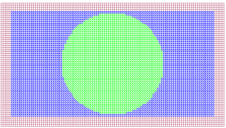
a) $\Omega$	b) $\Omega_{FEM}=\Omega_{1}\cup\Omega_{2}$

Figure 1: a) Computational mesh used in the domain decomposition of the domain $\Omega=\Omega_{FEM}\cup\Omega_{FDM}$. b) The finite element mesh in $\Omega_{FEM}=\Omega_{1}\cup\Omega_{2}$.

Exact $\rho(x)$
Test 1	Test 2	Test 3	Test 4
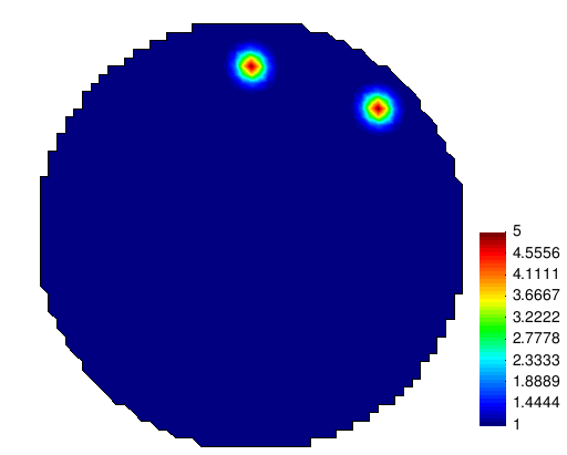
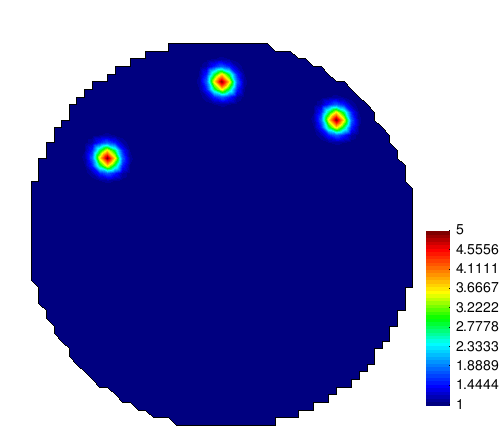
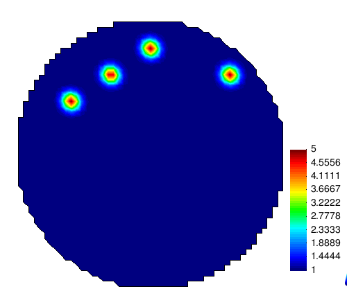
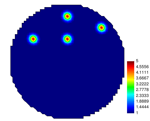
Exact $p(x)$
Test 1	Test 2	Test 3	Test 4

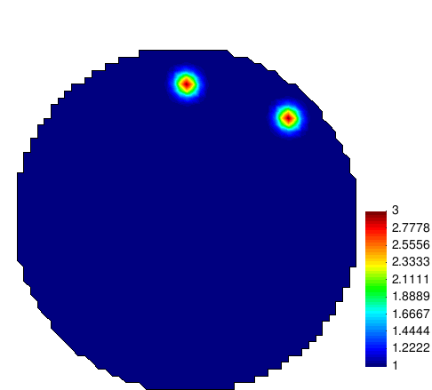
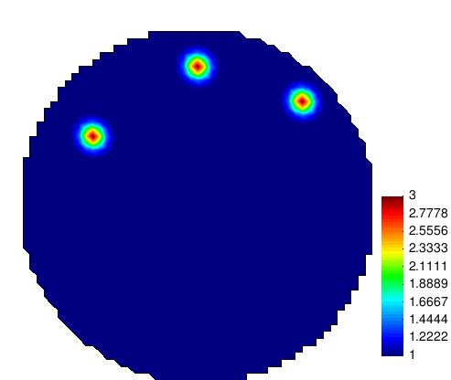
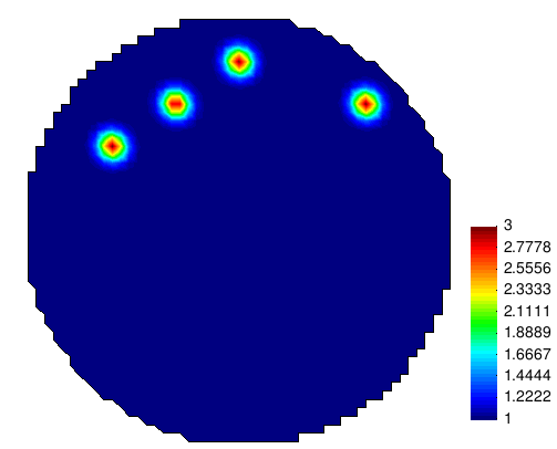
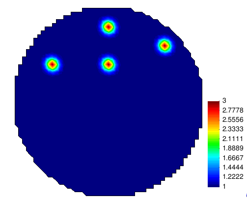
Figure 2: Exact Gaussian functions $\rho(x)$ and $p(x)$ in $\Omega_{1}$ in different tests.

Test 1
$\rho(x),\delta=3\%$	$\rho(x),\delta=10\%$	$p(x),\delta=3\%$	$p(x),\delta=10\%$
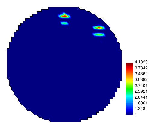
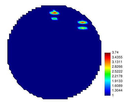
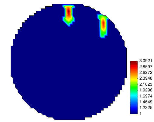
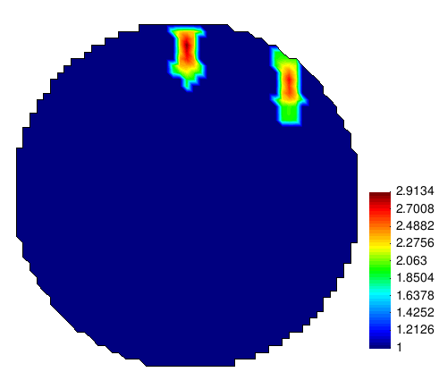
Test 2
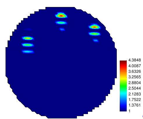
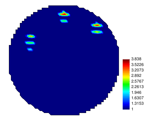
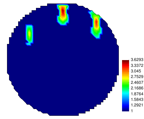
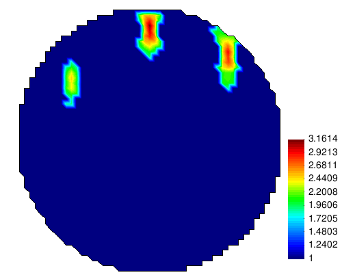
Test 3
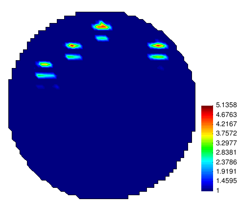
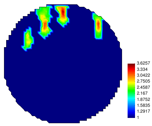
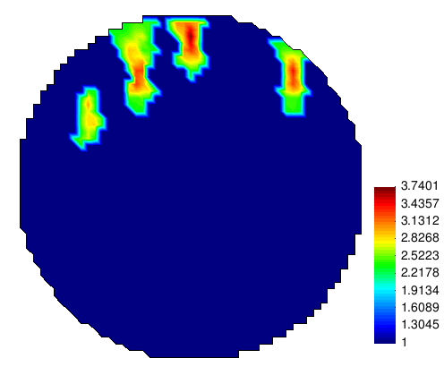
Test 4

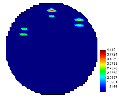
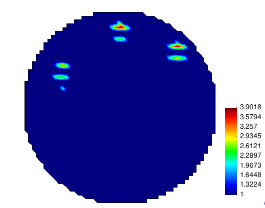
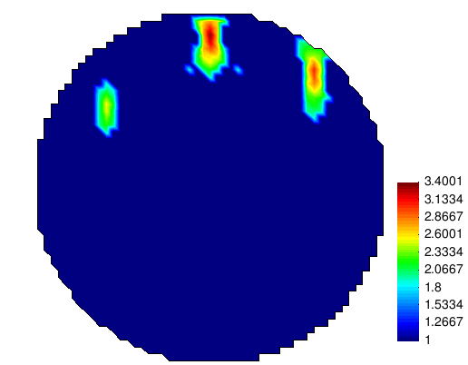
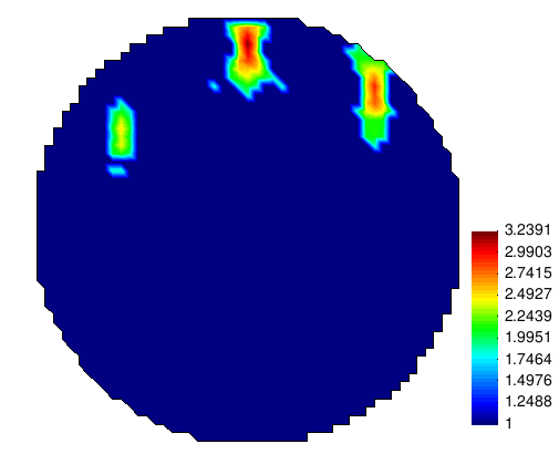
Figure 3: Reconstructions obtained in Tests 1-4 on a coarse mesh for different noise levels $\delta$ in data.

4 Numerical Studies

In this section, we present numerical simulations of the reconstruction of two unknown functions $\rho(x)$ and $p(x)$ of the equation (1.1) using the domain decomposition method of [3].

To do that we decompose the computational domain $\Omega$ into two subregions $\Omega_{FEM}$ and $\Omega_{FDM}$ such that $\Omega=\Omega_{FEM}\cup\Omega_{FDM}$ with two layers of structured overlapping nodes between these domains, see Figure 1 and Figure 2 of [4] for details about communication between $\Omega_{FEM}$ and $\Omega_{FDM}$. We will apply in our computations the finite element method (FEM) in $\Omega_{FEM}$ and the finite difference method (FDM) in $\Omega_{FDM}$. We also decompose the domain $\Omega_{FEM}$ into two different domains $\Omega_{1},\Omega_{2}$ such that $\Omega_{FEM}=\Omega_{1}\cup\Omega_{2}$ which are intersecting only by their boundaries, see Figure 1. We use the domain decomposition approach in our computations since it is efficiently implemented in the high performance software package WavES [47] using C++ and PETSc [45]. For further details about construction of $\Omega_{FDM}$ and $\Omega_{FEM}$ domains as well as the domain decomposition method we refer to [3].

The boundary $\partial\Omega$ of the domain $\Omega$ is such that $\partial\Omega=\partial_{1}\Omega\cup\partial_{2}\Omega\cup\partial_{3}\Omega$ where $\partial_{1}\Omega$ and $\partial_{2}\Omega$ are, respectively, top and bottom parts of $\Omega$, and $\partial_{3}\Omega$ is the union of left and right sides of this domain. We will collect time-dependent observations $\Gamma_{1}:=\partial_{1}\Omega\times(0,T)$ at the backscattering side $\partial_{1}\Omega$ of $\Omega$. We also define $\Gamma_{1,1}:=\partial_{1}\Omega\times(0,t_{1}]$, $\Gamma_{1,2}:=\partial_{1}\Omega\times(t_{1},T)$, $\Gamma_{2}:=\partial_{2}\Omega\times(0,T)$ and $\Gamma_{3}:=\partial_{3}\Omega\times(0,T)$.

We have used the following model problem in all computations:

$$\begin{split}\rho(x)\partial_{t}^{2}u(x,t)-\mbox{div}\thinspace((p(x)\nabla u(x,t))&=0~{}\mbox{in}~{}~{}\Omega_{T},\\ u(x,0)=a(x),~{}~{}~{}u_{t}(x,0)&=0~{}\mbox{in}~{}~{}\Omega,\\ \partial_{n}u&=f(t)~{}\mbox{on}~{}\Gamma_{1,1},\\ \partial_{n}u&=-\partial_{t}u~{}\mbox{on}~{}\Gamma_{1,2},\\ \partial_{n}u&=-\partial_{t}u~{}\mbox{on}~{}\Gamma_{2},\\ \partial_{n}u&=0~{}\mbox{on}~{}\Gamma_{3}.\\ \end{split}$$ (4.1)

In (4.1) the function $f(t)$ represents the single direction of a plane wave which is initialized at $\partial_{1}\Omega$ in time $t=[0,2.0]$ and is defined as

$$\begin{split}f(t)=\left\{\begin{array}[]{ll}\sin\left(\omega_{f}t\right),&\text{ if }t\in\left(0,\frac{2\pi}{\omega_{f}}\right),\\ 0,&\text{ if }t>\frac{2\pi}{\omega_{f}}.\end{array}\right.\end{split}$$ (4.2)

We initialize initial condition $a(x)$ at the boundary $\partial_{1}\Omega$ as

$$\begin{split}u(x,0)&=f_{0}(x)={\rm e}^{-(x_{1}^{2}+x_{2}^{2}+x_{3}^{3})}\cdot\cos t|_{t=0}={\rm e}^{-(x_{1}^{2}+x_{2}^{2}+x_{3}^{3})}.\end{split}$$ (4.3)

We assume that both functions $\rho(x)=p(x)=1$ are known inside $\Omega_{FDM}\cup\Omega_{2}$. The goal of our numerical tests is to reconstruct simultaneously two smooth functions $\rho(x),p(x)$ of the domain $\Omega_{1}$ of Figure 1. The main feature of these functions is that they model inclusions of a very small sizes what can be of practical interest in real-life applications.

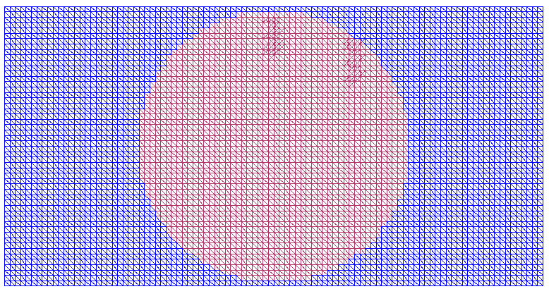
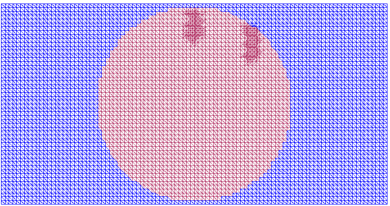
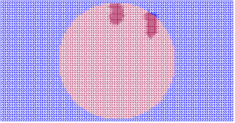
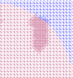
adaptively refined meshes zoomed once refined mesh twice refined mesh three times refined mesh
$\rho(x),\delta=3\%$	$\rho(x),\delta=10\%$	$p(x),\delta=3\%$	$p(x),\delta=10\%$

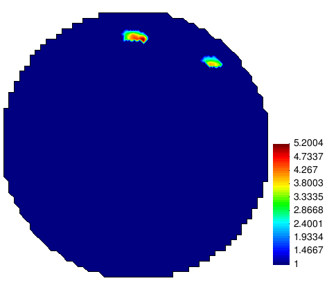
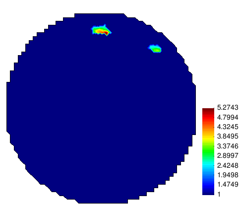
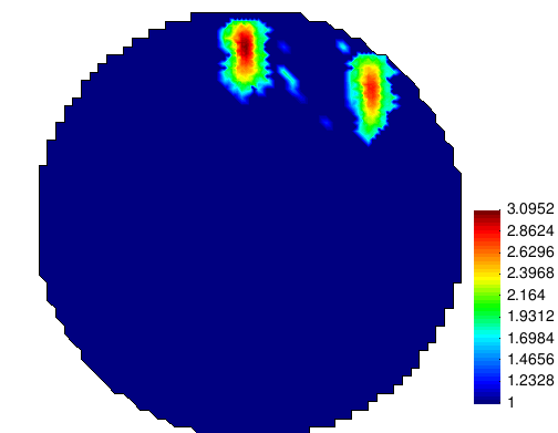
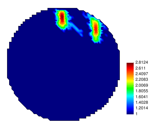
Figure 4: Test 1: reconstructions obtained on three times adaptively refined mesh for different noise levels $\delta$ in data.

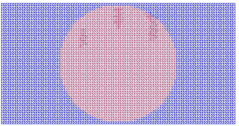
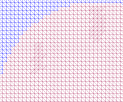
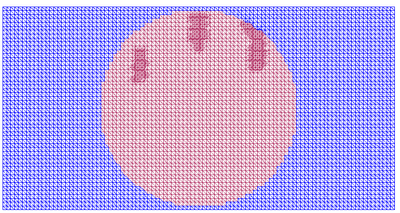
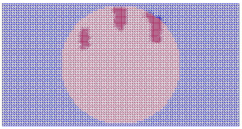
adaptively refined meshes zoomed once refined mesh twice refined mesh three times refined mesh
$\rho(x),\delta=3\%$	$\rho(x),\delta=10\%$	$p(x),\delta=3\%$	$p(x),\delta=10\%$

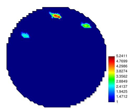
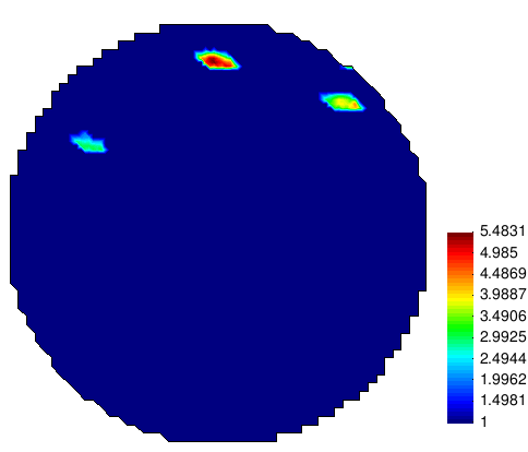
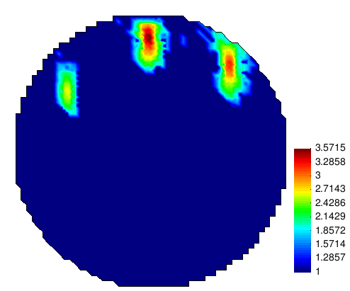
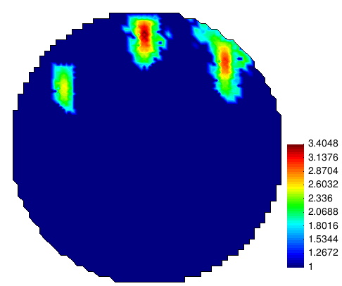
Figure 5: Test 2: reconstructions obtained on two times adaptively refined mesh for different noise levels $\delta$ in data.

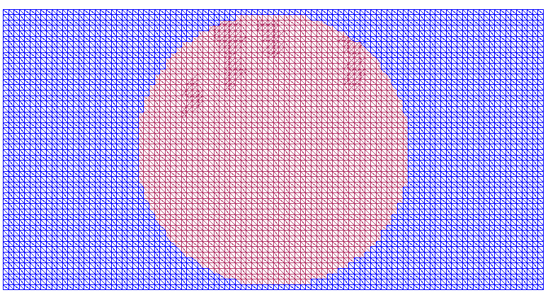
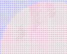
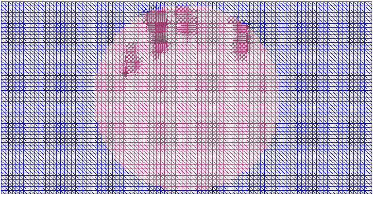
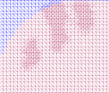
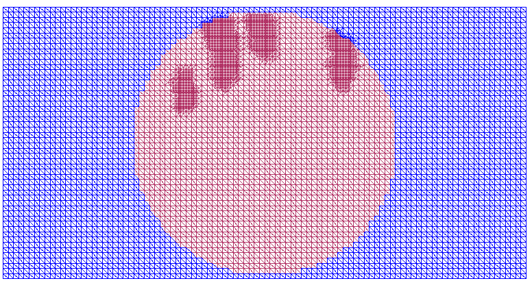
adaptively refined meshes zoomed once refined mesh twice refined mesh three times refined mesh
$\rho(x),\delta=3\%$	$\rho(x),\delta=10\%$	$p(x),\delta=3\%$	$p(x),\delta=10\%$

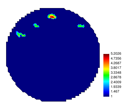
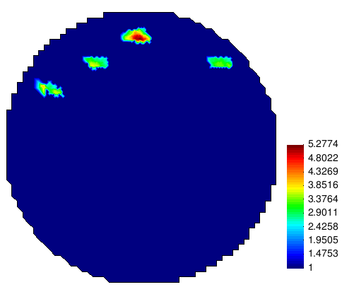
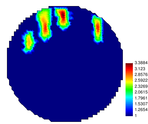
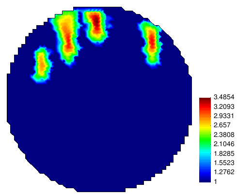
Figure 6: Test 3: reconstructions obtained on three times adaptively refined mesh for different noise levels $\delta$ in data.

We set the dimensionless computational domain $\Omega$ in the domain decomposition as

$$\Omega=\left\{x=(x_{1},x_{2}):x_{1}\in(-1.1,1.1),x_{2}\in(-0.62,0.62)\right\},$$

and the domain $\Omega_{FEM}$ as

$$\Omega_{FEM}=\left\{x=(x_{1},x_{2}):x_{1}\in(-1.0,1.0),x_{2}\in(-0.52,0.52)\right\}.$$

We choose the mesh size $h=0.02$ in $\Omega=\Omega_{FEM}\cup\Omega_{FDM}$, as well as in the overlapping regions between FE/FD domains.

We assume that our two functions $\rho(x),p(x)$ belongs to the set of admissible parameters

$$\begin{split}M_{\rho}&=\{\rho\in C^{2}(\overline{\Omega});~{}1\leq\rho(x)\leq 10\},\\ M_{p}&=\{p\in C^{2}(\overline{\Omega});~{}1\leq p(x)\leq 5\}.\end{split}$$ (4.4)

We define now our coefficient inverse problem which we use in computations.

Inverse Problem (IP) Assume that the functions $\rho(x),p(x)$  of the model problem (4.1) are unknown. Let these functions satisfy conditions (4.4,) and $\rho(x)=1,p(x)=1$ in the domain $\Omega\backslash\Omega_{\rm FEM}$. Determine the functions $\rho(x),p(x)$ for $x\in\Omega\backslash\Omega_{\rm FDM},$  assuming that the following function $\tilde{u}\left(x,t\right)$ is known

$$u\left(x,t\right)=\tilde{u}\left(x,t\right),\forall\left(x,t\right)\in\Gamma_{1}.$$ (4.5)

To determine both coefficients $\rho(x),p(x)$ in inverse problem IP we minimize the following Tikhonov functional

$$\begin{split}J(\rho(x),p(x))&:=J(u,\rho,p)=\frac{1}{2}\int_{\Gamma_{1}}(u-\tilde{u})^{2}z_{\delta}(t)dsdt\\ &+\frac{1}{2}\alpha_{1}\int_{\Omega}(\rho-\rho_{0})^{2}~{}~{}dx+\frac{1}{2}\alpha_{2}\int_{\Omega}(p-p_{0})^{2}~{}~{}dx.\end{split}$$ (4.6)

Here, $\tilde{u}$ is the observed function $u$ in time at the backscattered boundary $\partial_{1}\Omega$, the function $u$ satisfy the equations (4.1) and thus depends on $\rho,p$, $\rho_{0},p_{0}$ are the initial guesses for $\rho,p$, correspondingly, and $\alpha_{i},i=1,2$, are regularization parameters. We take $\rho_{0}=1,p_{0}=1$ at all points of the computational domain since previous computational works [3, 10, 2, 7] as well as experimental works of [43, 44] have shown that a such choice gives good results of reconstruction. Here, $z_{\delta}(t)$ is a cut-off function chosen as in [3, 10, 7]. This function is introduced to ensure the compatibility conditions at $\overline{\Omega}_{T}\cap\left\{t=T\right\}$ for the adjoint problem, see details in [3, 10, 7].

To solve the minimization problem we take into account conditions (4.4) and introduce the Lagrangian

$$\begin{split}L(v)&=J(u,\rho,p)+\int_{\Omega}\int_{0}^{T}\lambda\Big{(}\rho\frac{\partial^{2}u}{\partial t^{2}}-\mbox{div}\thinspace(p\nabla u)\Big{)}~{}dxdt,\end{split}$$ (4.7)

where $v=(u,\lambda,\rho,p)$. Our goal is to find a stationary point of the Lagrangian with respect to $v$ satisfying $\forall\bar{v}=(\bar{u},\bar{\lambda},\bar{\rho},\bar{p})$

$$L^{\prime}(v;\bar{v})=0,$$ (4.8)

where $L^{\prime}(v;\cdot)$ is the Jacobian of $L$ at $v$. To find optimal parameters $\rho,p$ from (4.8) we use the conjugate gradient method with iterative choice of the regularization parameters $\alpha_{j},j=1,2$, in (4.6). More precisely, in all our computations we choose the regularization parameters iteratively as was proposed in [1], such that $\alpha^{n}_{j}=\alpha^{0}_{j}(n+1)^{-q}$, where $n$ is the number of iteration in the conjugate gradient method, $q\in(0,1)$ and $\alpha^{0}_{j}$ are initial guesses for $\alpha_{j},j=1,2$. Similarly with [35] we take $\alpha_{j}=\delta^{\zeta}$, where $\delta$ is the noise level and $\zeta$ is a small number taken in the interval $(0,1)$. Different techniques for the computation of a regularization parameter are presented in works [23, 30, 31, 46], and checking of performance of these techniques for the solution of our inverse problem can be challenge for our future research.

To generate backscattered data we solve the model problem (4.1) in time $T=[0,2.0]$ with the time step $\tau=0.002$ which satisfies to the CFL condition [21]. In order to check performance of the reconstruction algorithm we supply simulated backscattered data at $\partial_{1}\Omega$ by additive, as in [3, 10, 7], noise $\delta=3\%,10\%$. Similar results of reconstruction are obtained for random noise and they will be presented in the forthcoming publication.

Table 1. Computational results of the reconstructions on a coarse and on adaptively refined meshes together with computational errors in the maximal contrast of $\rho(x),p(x)$ in percents. Here, $N_{\rho}^{j},N_{p}^{j}$ denote the final number of iterations in the conjugate gradient method on $j$ times refined mesh for reconstructed functions $\rho$ and $p$, respectively.

Coarse mesh $\delta=3\%$ $\delta=10\%$ Case $\max_{\Omega_{1}}\rho$ error, % $N_{\rho}^{0}$ Test 1 4.13 17.4 13 Test 2 4.38 12.4 $15$ Test 3 5.14 2.8 $16$ Test 4 4.12 17.6 $14$ Case $\max_{\Omega_{1}}\rho$ error, % $N_{\rho}^{0}$ Test 1 3.74 25.2 12 Test 2 3.84 23.2 $13$ Test 3 5.08 1.6 $16$ Test 4 3.9 22 $13$ Case $\max_{\Omega_{1}}p$ error, % $N_{p}^{0}$ Test 1 3.09 3 $13$ Test 2 3.63 21 $15$ Test 3 3.63 21 $16$ Test 4 3.4 13.3 $14$ Case $\max_{\Omega_{1}}p$ error, % $N_{p}^{0}$ Test 1 2.9 3.33 $12$ Test 2 3.16 5.33 $13$ Test 3 3.74 24.67 $16$ Test 4 3.24 8 13 Adaptively refined mesh Case $\max_{\Omega_{1}}\rho$ error, % $N_{\rho}^{j}$ Test 1 5.2 4 $N_{\rho}^{3}=9$ Test 2 5.24 4.8 $N_{\rho}^{2}=6$ Test 3 5.2 4 $N_{\rho}^{3}=1$ Test 4 5.5 10 $N_{\rho}^{3}=8$ Case $\max_{\Omega_{1}}\rho$ error, % $N_{\rho}^{j}$ Test 1 5.3 6 $N_{\rho}^{3}=7$ Test 2 5.5 10 $N_{\rho}^{2}=10$ Test 3 5.28 5.6 $N_{\rho}^{3}=1$ Test 4 5.36 7.2 $N_{\rho}^{3}=8$ Case $\max_{\Omega_{1}}p$ error, % $N_{p}^{j}$ Test 1 3.1 3.33 $N_{p}^{3}=9$ Test 2 3.57 19 $N_{p}^{2}=6$ Test 3 3.39 13 $N_{p}^{3}=1$ Test 4 3.4 13.3 $N_{p}^{3}=14$ Case $\max_{\Omega_{1}}p$ error, % $N_{p}^{j}$ Test 1 2.8 6.67 $N_{p}^{3}=7$ Test 2 3.4 13.3 $N_{p}^{2}=9$ Test 3 3.49 16.3 $N_{p}^{3}=1$ Test 4 3.26 8.67 $N_{p}^{3}=10$

4.1 Test 1

In this test we present numerical results of the simultaneous reconstruction of two functions $\rho(x)$ and $p(x)$ given by

$$\begin{split}\rho(x)=1.0&+4.0\cdot{\rm e}^{-((x_{1}-0.3)^{2}+{(x_{2}-0.3)}^{2})/0.001}\\ &+4.0\cdot{\rm e}^{-(x_{1}^{2}+{(x_{2}-0.4)}^{2})/0.001},\\ p(x)=1.0&+2.0\cdot{\rm e}^{-((x_{1}-0.3)^{2}+{(x_{2}-0.3)}^{2})/0.001}\\ &+2.0\cdot{\rm e}^{-(x_{1}^{2}+{(x_{2}-0.4)}^{2})/0.001},\\ \end{split}$$ (4.9)

which are presented in Figure  2.

Figures 3 show results of the reconstruction on a coarse mesh with additive noise $\delta=3\%,10\%$ in data. We observe that the location of both functions $\rho,p$ given by (4.9) is imaged correctly. We refer to Table 1 for the reconstruction of the contrast in both functions.

To improve contrast and shape of the reconstructed functions $\rho(x)$ and $p(x)$ we run computations again using an adaptive conjugate gradient method similar to the one of [7]. Figure 4 and Table 1 show results of reconstruction on the three times locally refined mesh. We observe that we achieve better contrast for both functions $\rho(x)$ and $p(x)$, as well as better shape for the function $\rho(x)$.

4.2 Test 2

In this test we present numerical results of the reconstruction of the functions $\rho(x)$ and $p(x)$ given by three Gaussians shown in Figure  2 and given by

$$\begin{split}\rho(x)=1.0&+4.0\cdot{\rm e}^{-((x_{1}-0.3)^{2}+{(x_{2}-0.3)}^{2})/0.001}\\ &+4.0\cdot{\rm e}^{-(x_{1}^{2}+{(x_{2}-0.4)}^{2})/0.001}\\ &+4.0\cdot{\rm e}^{-((x_{1}+0.3)^{2}+{(x_{2}-0.2)}^{2})/0.001},\\ p(x)=1.0&+2.0\cdot{\rm e}^{-((x_{1}-0.3)^{2}+{(x_{2}-0.3)}^{2})/0.001}\\ &+2.0\cdot{\rm e}^{-(x_{1}^{2}+{(x_{2}-0.4)}^{2})/0.001}\\ &+2.0\cdot{\rm e}^{-((x_{1}+0.3)^{2}+{(x_{2}-0.2)}^{2})/0.001}.\end{split}$$ (4.10)

Figures 3 show results of the reconstruction on a coarse mesh with additive noise $\delta=3\%,10\%$ in data. We observe that the location of three Gaussians for both functions $\rho,p$ is imaged correctly, see Table 1 for the reconstruction of contrast in these functions.

To improve contrast and shape of the reconstructed functions $\rho(x)$ and $p(x)$ we run computations again using an adaptive conjugate gradient method similar to the one of [7]. Figure 5 and Table 1 show results of reconstruction on the two times locally refined mesh. We observe that we achieve better contrast for both functions $\rho(x)$ and $p(x)$, as well as better shape for the function $\rho(x)$. Results on the three times refined mesh were similar to the results obtained on a two times refined mesh, and we are not presenting them here.

4.3 Test 3

This test presents numerical results of the reconstruction of the functions $\rho(x)$ and $p(x)$ given by four different Gaussians shown in Figure  2 and given by

$$\begin{split}\rho(x)=1.0&+4.0\cdot{\rm e}^{-((x_{1}-0.3)^{2}+{(x_{2}-0.3)}^{2})/0.001}\\ &+4.0\cdot{\rm e}^{-(x_{1}^{2}+{(x_{2}-0.4)}^{2})/0.001}\\ &+4.0\cdot{\rm e}^{-((x_{1}+0.3)^{2}+{(x_{2}-0.2)}^{2})/0.001}\\ &+4.0\cdot{\rm e}^{-((x_{1}+0.15)^{2}+{(x_{2}-0.3)}^{2})/0.001},\\ p(x)=1.0&+2.0\cdot{\rm e}^{-((x_{1}-0.3)^{2}+{(x_{2}-0.3)}^{2})/0.001}\\ &+2.0\cdot{\rm e}^{-(x_{1}^{2}+{(x_{2}-0.4)}^{2})/0.001}\\ &+2.0\cdot{\rm e}^{-((x_{1}+0.3)^{2}+{(x_{2}-0.2)}^{2})/0.001}\\ &+2.0\cdot{\rm e}^{-((x_{1}+0.15)^{2}+{(x_{2}-0.3)}^{2})/0.001}.\end{split}$$ (4.11)

Figures 3 show results of the reconstruction of four Gaussians on a coarse mesh with additive noise $\delta=3\%,10\%$ in data. We have obtained similar results as in the two previous tests: the location of four Gaussians for both functions $\rho,p$ already on a coarse mesh is imaged correctly. However, as follows from the Table 1, the contrast should be improved. Again, to improve the contrast and shape of the Gaussians we run an adaptive conjugate gradient method similar to one of [7]. Figure 6 shows results of reconstruction on the three times locally refined mesh. Using Table 1 we observe that we achieve better contrast for both functions $\rho(x)$ and $p(x)$, as well as better shape for the function $\rho(x)$.

4.4 Test 4

In this test we tried to reconstruct four Gaussians shown in Figure  2 and given by

$$\begin{split}\rho(x)=1.0&+4.0\cdot{\rm e}^{-((x_{1}-0.3)^{2}+{(x_{2}-0.3)}^{2})/0.001}\\ &+4.0\cdot{\rm e}^{-(x_{1}^{2}+{(x_{2}-0.4)}^{2})/0.001}\\ &+4.0\cdot{\rm e}^{-((x_{1}+0.3)^{2}+{(x_{2}-0.2)}^{2})/0.001}\\ &+4.0\cdot{\rm e}^{-(x_{1}^{2}+{(x_{2}-0.2)}^{2})/0.001},\\ p(x)=1.0&+2.0\cdot{\rm e}^{-((x_{1}-0.3)^{2}+{(x_{2}-0.3)}^{2})/0.001}\\ &+2.0\cdot{\rm e}^{-(x_{1}^{2}+{(x_{2}-0.4)}^{2})/0.001}\\ &+2.0\cdot{\rm e}^{-((x_{1}+0.3)^{2}+{(x_{2}-0.2)}^{2})/0.001}\\ &+2.0\cdot{\rm e}^{-(x_{1}^{2}+{(x_{2}-0.2)}^{2})/0.001}.\end{split}$$ (4.12)

We observe that two Gaussians in this example are located one under another one. Thus, backscattered data from these two Gaussians will be superimposed and thus, we expect to reconstruct only three Gaussians from four.

Figure 3 shows results of the reconstruction of these four Gaussians on a coarse mesh with additive noise $\delta=3\%,10\%$ in data. As expected, we could reconstruct only three Gaussians from four, see Table 1 for reconstruction of the contrast in them. Even application of the adaptive algorithm can not give us the fourth Gaussian. However, the contrast in the reconstructed functions is improved, as in Test 3.

5 Conclusions

In this work we present theoretical and numerical studies of the reconstruction of two space-dependent functions $\rho(x)$ and $p(x)$ in a hyperbolic problem.
In the theoretical part of this work we derive a local Carleman estimate which allows to obtain a conditional Lipschitz stability inequality for the inverse problem formulated in section 1. This stability is very important for our subsequent numerical reconstruction of the two unknown functions $\rho(x)$ and $p(x)$ in the hyperbolic model (4.1).
In the numerical part we present a computational study of the simultaneous reconstruction of two functions $\rho(x)$ and $p(x)$ in a hyperbolic problem (4.1) from backscattered data using an adaptive domain decomposition finite element/difference method similar to one developed in [3, 7]. In our numerical tests, we have obtained stable reconstruction of the location and contrasts of both functions $\rho(x)$ and $p(x)$ for noise levels $\delta=3\%,10\%$ in backscattered data. Using results of Table 1 and Figures 4–6 we can conclude, that an adaptive domain decomposition finite element/finite difference algorithm significantly improves qualitative and quantitative results of the reconstruction obtained on a coarse mesh.

References

- [1] A. Bakushinsky, M. Y. Kokurin, and A. Smirnova, Iterative Methods for Ill-posed Problems, De Gruyter, Berlin, 2011.
- [2] L.Beilina, Adaptive Finite Element Method for a coefficient inverse problem for the Maxwell’s system, Applicable Analysis, 90 (2011), 1461–1479.
- [3] L. Beilina, Domain Decomposition finite element/finite difference method for the conductivity reconstruction in a hyperbolic equation, Communications in Nonlinear Science and Numerical Simulation, Elsevier, 2016, doi:10.1016/j.cnsns.2016.01.016
- [4] L. Beilina, Adaptive hybrid FEM/FDM methods for inverse scattering problems, Inverse Problems and Information Technologies, 1(3), 73–116, 2002.
- [5] L. Beilina, M. Cristofol, and S. Li, Uniqueness and stability of time and space-dependent conductivity in a hyperbolic cylindrical domain, arXiv:1607.01615.
- [6] L. Beilina, M. Cristofol, and K. Niinimäki, Optimization approach for the simultaneous reconstruction of the dielectric permittivity and magnetic permeability functions from limited observations, Inverse Problems and Imaging, 9 (2015), 1-25.
- [7] L. Beilina and S. Hosseinzadegan, An adaptive finite element method in reconstruction of coefficients in Maxwell’s equations from limited observations, Applications of Mathematics, 61(3) (2016), 253–286.
- [8] L. Beilina and C. Johnson, A posteriori error estimation in computational inverse scattering, Mathematical Models in Applied Sciences, 1 (2005), 23-35.
- [9] L. Beilina and M.V. Klibanov, Approximate Global Convergence and Adaptivity for Coefficient Inverse Problems, Springer-Verlag, Berlin, 2012.
- [10] L. Beilina and K. Niinimäki, Numerical studies of the Lagrangian approach for reconstruction of the conductivity in a waveguide, arXiv:1510.00499, 2015.
- [11] M. Bellassoued, Uniqueness and stability in determining the speed of propagation of second order hyperbolic equation with variable coefficients, Appl. Anal. 83 (2004), 983-1014.
- [12] M.Bellassoued, Global logarithmic stability in inverse hyperbolic problem by arbitrary boundary observation, Inverse Problems 20 (2004), 1033-1052.
- [13] M. Bellassoued, M. Cristofol, and E. Soccorsi, Inverse boundary value problem for the dynamical heterogeneous Maxwell’s system, Inverse Problems 28 (2012), 095009.
- [14] M. Bellassoued, O. Y. Imanuvilov, and M. Yamamoto, Inverse problem of determining the density and two Lame coefficients by boundary data, SIAM J. Math. Anal. 40 (2008), 238-265.
- [15] M. Bellassoued, D. Jellali and M. Yamamoto, Lipschitz stability in in an inverse problem for a hyperbolic equation with a finite set of boundary data, Applicable Analysis 87 (2008), 1105-1119.
- [16] M. Bellassoued and M. Yamamoto, Logarithmic stability in determination of a coefficient in an acoustic equation by arbitrary boundary observation, J. Math. Pures Appl. 85 (2006), 193-224.
- [17] M. Bellassoued and M. Yamamoto, Determination of a coefficient in the wave equation with a single measurement, Appl. Anal. 87 (2008), 901-920.
- [18] M. Bellassoued and M. Yamamoto, Carleman Estimates and Applications to Inverse Problems for Hyperbolic Systems, Springer-Japan, to appear.
- [19] A.L. Bugkheim and M.V.Klibanov, Global uniqueness of class of multidimentional inverse problems, Soviet Math. Dokl. 24 (1981), 244-247.
- [20] J. Cheng, V. Isakov, M. Yamamoto, and Q. Zhou, Lipschitz stability in the lateral Cauchy problem for elasticity system, J. Math. Kyoto Univ. 43 (2003), 475-501.
- [21] R. Courant, K. Friedrichs and H. Lewy, On the partial differential equations of mathematical physics, Journal of Research and Development, 11(2) (1967), 215–234.
- [22] Y. T. Chow and J. Zou, A numerical method for reconstructing the coefficient in a wave equation, Numerical Methods for Partial Differential Equations 31 (2015), 289–307.
- [23] H. W. Engl, M. Hanke and A. Neubauer, Regularization of Inverse Problems, Kluwer, Boston, 2000.
- [24] O. Y. Imanuvilov, On Carleman estimates for hyperbolic equations, Asymptotic Analysis 32 (2002), 185-220.
- [25] O. Y. Imanuvilov, V. Isakov and M. Yamamoto, An inverse problem for the dynamical Lamé system with two sets of boundary data, Comm. Pure Appl. Math. 56 (2003), 1366-1382.
- [26] O. Y. Imanuvilov and M. Yamamoto, Global uniqueness and stability in determining coefficients of wave equations, Comm. Partial Differential Equations 26 (2001), 1409-1425.
- [27] O. Y. Imanuvilov and M. Yamamoto, Global Lipschitz stability in an inverse hyperbolic problem by interior observations, Inverse Problems 17 (2001), 717-728.
- [28] O. Y. Imanuvilov and M. Yamamoto, Determination of a coefficient in an acoustic equation with single measurement, Inverse Problems 19 (2003), 157-171.
- [29] V. Isakov, Inverse Problems for Partial Differential Equations, Springer-Verlag, Berlin, 1998, 2006.
- [30] K. Ito, B. Jin, and T. Takeuchi, Multi-parameter Tikhonov regularization, Methods and Applications of Analysis, 18 (2011), 31-46.
- [31] B. Kaltenbacher, A. Neubauer, and O. Scherzer. Iterative Regularization Methods for Nonlinear Problems, de Gruyter, Berlin, 2008.
- [32] M. V. Klibanov, Inverse problems in the ”large” and Carleman bounds, Differential Equations, 20 (1984), 755-760.
- [33] M. V. Klibanov, Inverse problems and Carleman estimates, Inverse Problems, 8(1992), 575-596.
- [34] M. V. Klibanov, Carleman estimates for global uniqueness, stability and numerical methods for coefficient inverse problems, J. Inverse Ill-Posed Probl., 21 (2013), 477-560.
- [35] M. V. Klibanov, A. B. Bakushinsky, L. Beilina, Why a minimizer of the Tikhonov functional is closer to the exact solution than the first guess, Journal of Inverse and Ill - Posed Problems, 19 (2011), 83-105.
- [36] M. V. Klibanov and A. Timonov, Carleman Estimates for Coefficient Inverse Problems and Numerical Applications, VSP, Utrecht, 2004.
- [37] M. V. Klibanov and M. Yamamoto, Lipschitz stability of an inverse problem for an acoustic equation, Appl. Anal., 85 (2006), 515-538.
- [38] S. Li, An inverse problem for Maxwell’s equations in bi-isotropic media, SIAM Journal on Mathematical Analysis, 37 (2005), 1027–1043.
- [39] S. Li and M. Yamamoto, An inverse source problem for Maxwell’s equations in anisotropic media, Applicable Analysis, 84 (2005), 1051–1067.
- [40] S. Li and M. Yamamoto, An inverse problem for Maxwell’s equations in anisotropic media in two dimensions, Chin. Ann. Math. Ser B 28 (2007), 35-54.
- [41] J.-L. Lions, Controlabilité Exacte, Perturbations et Stabilisation des Système Distribués, Masson, Paris, 1988.
- [42] J.-L. Lions and E. Magenes, Non-Homogeneous Boundary Value Problems and Applications, Berlin, Springer, 1972.
- [43] C. Eyraud, J.-M. Geffrin, and A. Litman, 3-D imaging of a microwave absorber sample from microwave scattered field measurements, IEEE Microwave and Wireless Components Letters, 25(7)(2015), 472–474.
- [44] T. M. Grzegorczyk, P. M. Meaney, P. A. Kaufman, R. M. diFlorio Alexander, and K.D. Paulsen, Fast 3-d tomographic microwave imaging for breast cancer detection, IEEE Trans Med Imaging, 31 (2012), 1584–1592.
- [45] PETSc, Portable, Extensible Toolkit for Scientific Computation, http://www.mcs.anl.gov/petsc/
- [46] A. N. Tikhonov, A. V. Goncharsky, V. V. Stepanov, and A. G. Yagola, Numerical Methods for the Solution of Ill-Posed Problems, Kluwer, London, 1995.
- [47] WavES, the software package, http://www.waves24.com
- [48] M. Yamamoto, Uniqueness and stability in multidimensional hyperbolic inverse problems, J. Math. Pures Appl., 78 (1999), 65-98.