Transport in the cat’s eye flow on intermediate time scales

Abstract

We consider the advection-diffusion transport of tracers in a one-parameter family of plane periodic flows where the patterns of streamlines feature regions of confined circulation in the shape of “cat’s eyes”, separated by meandering jets with ballistic motion inside them. By varying the parameter, we proceed from the regular two-dimensional lattice of eddies without jets to the sinusoidally modulated shear flow without eddies. When a weak thermal noise is added, i.e. at large Péclet numbers, several intermediate time scales arise, with qualitatively and quantitatively different transport properties: depending on the parameter of the flow, the initial position of a tracer, and the aging time, motion of the tracers ranges from subdiffusive to super-ballistic. Extensive numerical simulations of the aged mean squared displacement for different initial conditions are compared to a theory based on a Lévy walk that describes the intermediate-time ballistic regime. Interplay of the walk process with internal circulation dynamics in the trapped state results at intermediate time scale in non-monotonic characteristics of aging.

I Introduction

In hydrodynamics, the global transport properties of complicated flow patterns are derived from (often nontrivial) spatial averages over the local geometry of the velocity field. Regions of circulation (eddies, vortices) and the far-reaching jets belong to the basic building blocks of many two-dimensional flow patterns. In laminar jets, the tracer particles are advected over large distances. In contrast, a tracer captured inside an eddy stays localized for a long time (in the absence of molecular diffusion, forever). In 1880, Lord Kelvin (Sir William Thomson) described the inviscid plane vortex street flanked by regions of translational motion. He portrayed a pattern in which two stripes with opposite directions of translational velocities were “separated $[\dots]$ by a cat’s eye border pattern of elliptic whirls” Kelvin . In the context of two-dimensional transport, it is convenient to replace a single vortex street by a spatially periodic stationary pattern of vortices and jets. Below we use for this purpose the so-called “cat’s eye flow”, introduced in Childress1989 for studies of hydromagnetic effects. This model allows us to vary, by means of the single parameter, the relative areas occupied by the eddies and by the jets. In the limit of shrinking jets, the pattern turns into the pure cellular flow, i.e. a periodic arrangement of eddies divided by the separatrices connecting stagnation points. The separatrices form the cell borders: as long as molecular diffusion is neglected, they stay impenetrable for the tracers. With diffusion taken into account, all flow regions become accessible for tracers, and their transport possesses a hierarchy of timescales: the short and intermediate times at which the starting position of a tracer (near the eddy center, close to a separatrix, etc.) matters, and the final asymptotic state in which information about the starting configuration has been effectively erased by diffusion. For the case of very small molecular diffusion, a formal mathematical distinction between intermediate timescales was suggested in Fannjiang_2002 where transport in absence of mean drift was viewed as a superposition of an appropriate random continuous martingale process and the nearly periodic fluctuation. Two characteristic times were introduced: the “martingale time”, defined as the ratio of the variance of fluctuation to the effective diffusivity, and the “dissipation time” at which the increments of the martingale become approximately stationary. Over long times, the martingale component dominates the behavior: “the longer the timescale, the less anomalous the scaling is” Fannjiang_2002 . Physically, different characteristic times are related to typical timescales of deterministic circulation as well as to average durations of diffusive passages across various building blocks of the flow pattern.

Cellular flows often serve as prime examples of systems showing subdiffusion for intermediate times, see Bouchaud ; Isichenko and references therein. From the point of view of transport, these systems have much in common with combs where one-dimensional motion along the backbone or spine is interrupted by motion along the teeth in the transverse direction. Movement along the backbone is modeled by continuous time random walks (CTRW) with power law waiting time densities. If the stages of propagation along the teeth as well as of circulation inside the eddies are regarded as time intervals spent in a trapped state, then diffusion in cellular flows corresponds to combs with finite tooth length and to CTRW with power law waiting time distributions possessing exponential cutoffs. These upper cutoffs originate in the typical maximal time needed to diffuse across an eddy. Like in other CTRW models with power law waiting times, the properties of the diffusion depend on the aging time and the initial conditions.

In cellular flows with weak molecular diffusion, see Pomeau ; Childress ; Soward ; Shraiman ; RosenbluthEtAl , the intermediate and the final asymptotics are of the main interest. The final asymptotics, as predicted by homogenization theory Majda , is diffusive, and here the recent effort has been put into the quantitative description. In flows without jets, like in Pomeau or in the eddy lattice flow PoeschkeEtAl2016 , the intermediate asymptotics is subdiffusive IyerNovikov ; HairerEtAl . In flows with jets (“channels” in terminology of Fannjiang ), this intermediate asymptotics corresponds to Lévy walks interrupted by rests. Before addressing the complex geometry of experimentally available flows SolomonEtAl1993 ; SolomonEtAl1994 ; WeeksEtAl1996 , it seems reasonable to perform a thorough study of a simpler variant: a two-dimensional periodic flow pattern of the “cat’s eye flow” Kelvin ; Childress1989 ; Fannjiang . Below, similar to our previous work on the eddy lattice flow PoeschkeEtAl2016 , we demonstrate that for tracers starting on the edge of the jet, the transport by this flow pattern for intermediate times can indeed be modeled as a Lévy walk (LW), with eddies in the role of traps, and jets viewed as a transport mode in the LW scheme (see ZaburdaevEtAl and references therein). This conclusion is corroborated by comparison of theoretical estimates with results of our extensive numerical simulations. However, due to the presence of internal circulation dynamics in the trapped state, the model based on the flow possesses a richer behavior than a simple Lévy walk model would suggest, which is manifested in its very different aging properties. In contrast to the well understood aging in LW Barkai ; Magdziarz , the cat’s eye flow displays strong dependence on the initial conditions and a set of unusual aging behaviors. Like in the eddy lattice, transport by the flow is more complicated than its random walk representation! We are aware neither of existing extensive numerical simulations of this system, nor of a comparison of numerics with theoretical predictions.

Below, in Sec. II we discuss and illustrate the basic features of the cat’s eye flow pattern. The subsequent Sec. III focuses on the different time scales for the mean squared displacement of tracer particles in the system. In Sec. IV we present and discuss the results of numerical simulations. Finally, in Sec. V we sum up our findings. Some details of the theoretical description are contained in the appendix.

II The flow

Dynamics of a tracer in the plane cat’s eye flow obeys the stochastic differential equation

$$\dot{\mathbf{r}}=\mathrm{rot}\,(0,0,\psi_{\mathrm{Cat}}(\mathbf{r}))+\sqrt{2D}\bm{\xi}$$ (1)

with the two-dimensional footnote1 stream function

$$\psi_{\mathrm{Cat}}(x,y)=u\,a\left(\sin\left(\frac{x}{a}\right)\sin\left(\frac{y}{a}\right)+A\cos\left(\frac{x}{a}\right)\cos\left(\frac{y}{a}\right)\right),$$ (2)

where $u$ is the characteristic velocity, $D$ is the molecular diffusivity and $\bm{\xi}=(\xi_{x},\xi_{y})$ is a vector of Gaussian noises with zero mean, unit variance and $\langle\xi_{x}(t)\xi_{x}(t^{\prime})\rangle=\langle\xi_{y}(t)\xi_{y}(t^{\prime})\rangle=\delta(t^{\prime}-t)$. The deterministic part of the flow pattern is periodic with respect to both coordinates and consists of elementary cells of the length and width $\pi a$. On taking $a$ as the spatial unit, ${a^{2}}/{D}$ as the unit of time, and introducing the Péclet number $\mathrm{Pe}={u\,a}/{D}$, the equations turn into

$$\dot{\mathbf{r}} = \mathrm{Pe}\;\mathrm{rot}\,(0,0,\Psi_{\mathrm{Cat}}(\mathbf{r}))+\sqrt{2}\bm{\xi}$$ (3)

$$\Psi_{\mathrm{Cat}}(x,y) = \sin x\sin y+A\cos x\cos y.$$ (4)

Thus the system is governed by two dimensionless parameters $A$ and Pe. We concentrate on the case $\mathrm{Pe}\gg 1$. The deterministic velocity components of the flow (4) are

$$\mathrm{Pe}^{-1}\dot{x} = \frac{\partial\Psi_{\mathrm{Cat}}}{\partial y}=\sin x\cos y-A\cos x\sin y$$ (5)

$$\mathrm{Pe}^{-1}\dot{y} = -\frac{\partial\Psi_{\mathrm{Cat}}}{\partial x}=-\cos x\sin y+A\sin x\cos y.$$

This flow pattern can be imposed in a layer of incompressible fluid with kinematic viscosity $\nu$ that obeys the Navier-Stokes equation, by applying a spatially periodic force, e.g. $\mathbf{F}=4\nu\sin x\cos y\,(\mathbf{e}_{x}+A\mathbf{e}_{y})$.

Formally, the parameter $A$ can assume arbitrary real values of either sign. However, it is sufficient to restrict analysis to the interval $0\leq A\leq 1$. A transformation $x\to\pi-x$ (or $y\to\pi-y$) is equivalent to the change of the sign of $A$, whereas a shift $x\to x+\pi/2$, $y\to y+\pi/2$ with simultaneous rescaling of time units by the factor $A$ is equivalent to the transformation $A\to 1/A$. For numerical investigations, we take the following values of $A$: $10^{-3},\,10^{-2},\,10^{-1},\,0.25,\,0.5,\,0.75,\,0.9,$ and $1$.

Regardless of the value of $A$, the flow possesses stagnation points at ($x=\pi m$, $y=\pi n$), and at ($x=\pi/2+\pi m$, $y=\pi/2+\pi n$), $m,n=0,\pm 1,\pm 2,\dots$. At $|A|<1$, the former points are hyperbolic fixed points (saddles) and the latter ones are elliptic fixed points (centers). At $|A|>1$, the reverse configuration of equilibria takes place. Exchange of stability between stagnation points occurs in the course of degenerate global bifurcation at $|A|=1$. At this parameter value, the straight lines $y=x+\pi n$, $n=\pm 1,\pm 2\dots$ turn into invariant continua of stagnation points, see straight red lines in Fig. 1 (a). In that case the system is transformed into a shear flow: the plane is partitioned into alternating regions of ballistic motion in opposite directions. At $A=0$, in contrast, the jets are absent and the entire plane is covered by cells with closed streamlines: the eddy lattice flow PoeschkeEtAl2016 . Isolines of the stream function (4) for several typical values of $A$ are presented in Fig. 1. The dashed curves, obtained by shifting by multiples of $\pi$ in both directions the curve

$$y(x)=\arctan\left(-A\cot(x)\right),$$ (6)

for $x\in[0,\pi]$, are the midlines of the jet regions in which ballistic motion takes place: along them, $\Psi_{\mathrm{Cat}}(x,y)$ vanishes. These jet regions are separated from the closed elliptic orbits by the isolines $|\Psi_{\mathrm{Cat}}|=A$: the separatrices are obtained by translating

$$y_{\pm}(x)=\arccos\left[\frac{A^{2}\cos x\pm\sqrt{1-A^{2}}\sin^{2}x}{A^{2}\cos^{2}x+\sin^{2}x}\right]$$ (7)

for $x\in[0,\pi]$ along both coordinates with $\pi$-periodicity, cf. the red curves that delineate cat’s eyes in Fig. 1. Here the plus (respectively minus) sign corresponds to the lower (respectively upper) boundary of the “cat’s eye”. At non-zero small values of $A$ the narrow curvy jets with alternating directions of unbounded motion are formed between the cells (Fig. 1f). As $A$ grows, these jets become thicker (Fig. 1e, Fig. 1d).

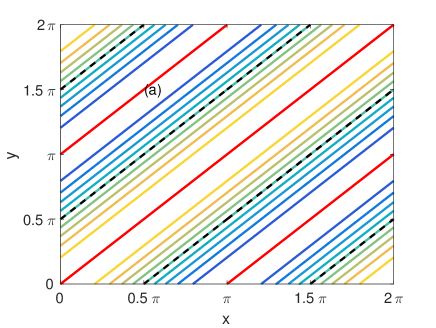
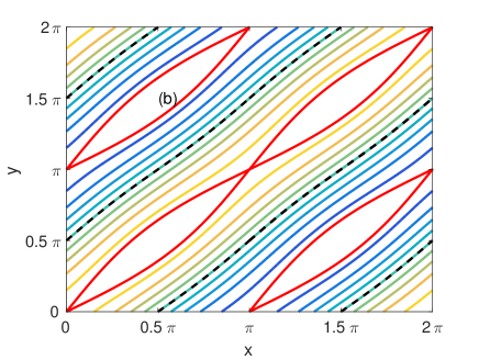
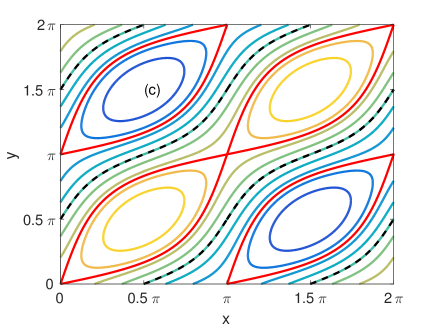
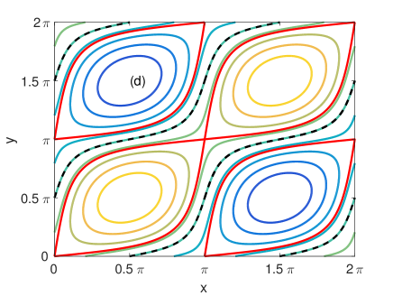
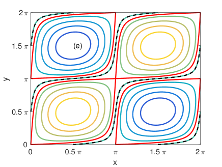
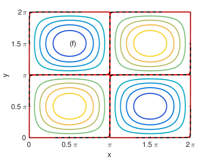
Figure 1: Contour plot of streamfunction (4) for (a) $A=1$, (b) $A=0.9$, (c) $A=0.5$, (d) $A=0.25$, (e) $A=10^{-1}$, and (f) $A=10^{-3}$. Yellow closed streamlines, e.g. lower left vortex, denote counterclockwise motion. Blue closed streamlines denote clockwise motion. For $A\to 1$ separatrices (red) between jets and eddies merge pairwise, the eddies cease to exist, and a shear flow with the sinusoidal velocity profile emerges. For $A\to 0$ pairs of separatrices (red) merge with the midline of the jet (black dashed) and become the edges of quadratic cells.

The flow is anisotropic: it possesses an axis of faster transport (shortened to “the axis” throughout this paper). Its direction corresponds to rotation of the coordinate system $(x,y)$ around the origin by $\pi/4$. In the rotated reference frame, the equations of motion are simplified: in terms of $x_{\pm}=x\pm y$, their deterministic part turns into

$$\dot{x}_{+} = \mathrm{Pe}\,(1+A)\sin x_{-},$$

$$\dot{x}_{-} = \mathrm{Pe}\,(1-A)\sin x_{+}.$$ (8)

At $A=1$ the value of $x_{-}$ becomes an integral of motion, and the plane gets foliated into the continuum of invariant straight lines. The velocity of motion along each of these lines is sinusoidally modulated across the continuum. In presence of diffusion, the (longitudinal) motion along $x_{+}$ has both deterministic and diffusive components, whereas the (transverse) motion along $x_{-}$ is purely diffusive. In contrast, at $A=0$, the pattern (II) turns into the conventional cellular flow. In terms of $x_{+}$ and $x_{-}$, the separatrix (7) becomes

$$x_{-}=\pm\arccos\left[\frac{(1-A)\cos x_{+}+2A}{1+A}\right],$$ (9)

hence the maximal width of the “eye”, in terms of original coordinates $x$ and $y$, is

$$\sqrt{2}\arccos\frac{3A-1}{1+A}.$$

The local velocity $v_{\rm s}$ along the separatrix is given by

$$v_{\rm s}^{2}(x_{+}) = 2\mathrm{Pe}^{2}(1-A)$$

$$\times\left[(A-1)\cos^{2}x_{+}-2A\cos x_{+}+A+1\right].$$

We take for the width of the jet channel the distance between the separatrices of adjacent saddle points, measured along the local normal direction to the midline $\Psi_{\mathrm{Cat}}=0$ of the jet, yielding a lengthy expression. As a function of the coordinate $x_{+}$, along the axis, the jet width oscillates between the sharp maximum

$$w_{\rm max}=\frac{1}{\sqrt{2}}\arccos\frac{1-3A}{1+A}$$ (11)

and the minimal value

$$w_{\rm min}=\frac{1+A}{\sqrt{1+A^{2}}}\arcsin\frac{2A}{1+A}$$ (12)

measured in units of the original coordinates. Both reproduce the exact width $\pi/\sqrt{2}$ of the jet for $A=1$.

At small values of $A$ the width displays a broad plateau around its minimal value. There, the minimum

$$w_{\rm min}\approx 2A+\frac{A^{3}}{3}+\ldots$$ (13)

can be used as a “typical” jet width. The linear approximation suffices for our purposes. At $A=1$ the deviation is 22%. For $A\leq 0.9$ it is 4% or less, fitting better for smaller values of $A$.

III Mean squared displacement

III.1 Characteristic times

We start from the analysis of the characteristic times involved in the motion of the particles. The treatment is analogous to the case of eddy lattices PoeschkeEtAl2016 , and the notation used is similar. In comparison to the eddy lattices with their two characteristic times:

• $t_{1}$ - the characteristic time of the deterministic transport over a single eddy,

• $t_{2}$ - the characteristic time to diffuse through a cell of the size $\pi a$,

here the third time,

• $t_{3}$ - the characteristic maximal time spent in a jet,

comes into play, making the picture more complex.

The estimates for the two first times are the same as in the eddy lattice flow, see PoeschkeEtAl2016 . Expressed in units of, respectively, Eq.(2) and Eq.(3), they are

$$t_{1}\simeq\frac{a}{u}=\frac{1}{\mathrm{Pe}}$$ (14)

and

$$t_{2}\simeq\frac{a^{2}}{D}\equiv 1,$$ (15)

and are interrelated via the Péclet number: $t_{1}=t_{2}/\mathrm{Pe}$. The third characteristic time is

$$t_{3}\simeq\frac{a^{2}}{D}w^{2}=t_{2}w^{2}$$ (16)

where $w$ is the characteristic width of the jet measured in units of $a$, i.e. the parameter $w$ itself is dimensionless. Note that

$$t_{3}=w^{2}\approx 4A^{2}$$ (17)

in our normalised units.

The waiting times in an eddy are given by a power law probability density function (normal Sparre-Andersen behavior)

$$\phi(t)\propto t^{-3/2}$$ (18)

between $t_{1}$ and $t_{2}$ with cutoffs both at short and at long times. The waiting time in a jet is given by a similar power law, but with the upper cutoff time $t_{3}$. The time $t_{1}$ corresponds essentially to the time resolution of the random walk scheme: behavior at shorter times is dominated by the local dynamics.

III.2 Transport regimes

When starting at the separatrix of the flow, three transport regimes can be observed. Here we describe them qualitatively; quantitative details are relegated to the subsequent section that presents the numerical simulations of the motion.

At short times $t<t_{1}$, a particle starting anywhere close to the separatrix, except for the immediate vicinity of the hyperbolic stagnation point, moves along the streamline with the local velocity close to $v_{s}$ and the average velocity $v$ of the order of Pe. This motion does not depend on whether the instantaneous position of the tracer is inside the jet or inside the eddy. The regime of motion is therefore ballistic: The mean squared displacement MSD of a particle grows as $\langle(\Delta R)^{2}\rangle\simeq v^{2}t^{2}$. The simulations confirm that at large Péclet numbers the typical velocities when moving close to the separatrix in the jet and in the eddy coincide, and are close to Pe: $v\approx\mathrm{Pe}$.

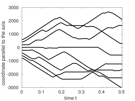
Figure 2: Coordinate parallel to the axis of the system at $\mathrm{Pe}=10^{4}$ and $A=0.5$ for a tracer starting at the separatrix. To resolve the trajectories optically at small values of $t$, a fictitious vertical shift between them has been introduced.

After the time $t_{1}$, provided both times $t_{2}$ and $t_{3}$ are considerably larger than $t_{1}$, i.e. $\mathrm{Pe}\,w^{2}\gg 1$, the second transport regime sets in. Like a preceding regime, this is still a ballistic transport, but a slower one: the prefactor is reduced to a quarter of its original size. At these times the particle might travel over several lattice cells. The translational motion in the jet corresponds to the transport mode of a Lévy walk scheme, whereas the confined motion in an eddy corresponds to the trapping event. Both stages can be visually identified in the trajectories in Fig. 2. The waiting time densities in the trapped and in the transport modes follow the same power-law asymptotics $\phi(t)\propto t^{-3/2}$. Such a Lévy walk scheme corresponds to the ballistic motion and the analysis within the Lévy walk formalism (see Appendix A) yields the expression for the growth of MSD:

$$\mathrm{MSD}(t)=\frac{1}{4}v^{2}t^{2}.$$ (19)

Subsequent regimes of ballistic transport for various values of $A$ are presented in Fig. 3. The crossover between them is visualized in Fig. 4, where it can be seen that the theoretical estimate for the change in the prefactor, given by Eq. (19), is well matched by simulations. The MSD is dominated by the longitudinal motion along the axis of the system. The (anomalous) transport in the system is strongly anisotropic since the motion in direction normal to the axis still takes place within just one eddy or jet. This motion cannot be captured by a coarse-grained random walk model, and will be discussed further on the basis of numerical results.

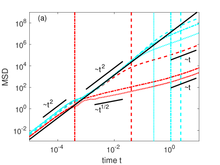
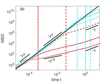
Figure 3: Temporal evolution of MSD for ensembles of tracers starting on the separatrix between the jet and the vortex at, respectively, $A=10^{-3}$ (lowest curve), $A=10^{-2}$, $A=10^{-1}$, $A=0.25$, $A=0.5$ (center curves), and $A=0.75$ (uppermost curve), compared to the asymptotic theory, Eq. (19) (black continuous). Time $t_{3}$ Eq. (17) is indicated by vertical lines. Panel (a): $10^{4}$ walks at Pe $=10^{4}$. Panel (b): $10^{3}$ walks at Pe $=10^{5}$. Velocity in both plots varies slightly with $A$ around $v\approx 0.75\,\mathrm{Pe}$. The intermediate ballistic regime occurs only if $t_{3}\gg t_{1}=1/\mathrm{Pe}$. Note that the curves in (a) are the black dashed lines in Figs. 5 and 6.

Figure 4: Crossover in prefactor of MSD between two regimes of ballistic transport. Rescaled curves from Fig. 3 (a) for $A=0.25$ (dotted), $A=0.5$ (dash-dotted), and $A=0.75$ (dashed). Horizontal lines indicate the values: $0.58$, $0.54$, $0.145$, and $0.135$. The MSD during the intermediate ballistic regime is about one quarter of its value during the initial ballistic regime, as predicted by theory, Eq. (19).

The behavior between the two larger times $t_{3}$ and $t_{2}$ is non-universal. In contrast, the terminal diffusion regime that sets in at long times $t>t_{2}$ is universal: it does not depend on initial conditions. In the remainder of this section we reproduce the estimates for directional coefficients of diffusion in the terminal regime, derived by Fannjiang and Papanicolaou Fannjiang .

At time and length scales corresponding to the terminal regime, the flow structure can be considered as a layered one, a parallel arrangement of jets and rows of eddies whose particular form practically ceases to play a role: the terminal diffusion coefficients are dominated by the times spent in the corresponding structures. A simple estimate is based on the assumption of constant thickness for those parallel layers: the exact form and the thickness modulation influence only numerical prefactors. For small $A$ the eddy lattice (EL) layers show isotropic diffusion with the diffusion coefficient

$$D_{\mathrm{EL}}\simeq\sqrt{uaD}=D\,\mathrm{Pe}^{1/2}.$$ (20)

The diffusion in the channel (jet) is strongly anisotropic. In the direction normal to the axis

$$D_{\bot}=D$$ (21)

holds, whereas in the parallel direction we have

$$D_{\|}\simeq u^{2}t_{3}=u^{2}\frac{a^{2}w^{2}}{D}=D\,\mathrm{Pe}^{2}w^{2}.$$ (22)

The terminal diffusion coefficient in the direction perpendicular to the axis is given by the harmonic mean of the corresponding local coefficients, i.e. it corresponds to a sequential switching of diffusivities (conductivities in electric terms)

$$D^{*}_{\bot}\simeq(D_{\mathrm{EL}}^{-1}(1-w)+D_{\bot}^{-1}w)^{-1}=\frac{D}{w+(1-w)\mathrm{Pe}^{-1/2}}.$$ (23)

For large $\mathrm{Pe}$ it is dominated by the first term in the denominator

$$D^{*}_{\bot}\simeq D/w\simeq D/A.$$ (24)

This effect takes place for $w>\mathrm{Pe}^{-1/2}$, which in the units $u=a=1$, used in Fannjiang , translates precisely into $A>\sqrt{D}$. The final diffusion coefficient in the direction parallel to the axis is the one for parallel switching of the diffusivities (conductivities)

$$D^{*}_{\|}\simeq D_{\mathrm{EL}}(1-w)+D_{\|}w=D[\mathrm{Pe}^{2}w^{3}+\mathrm{Pe}^{1/2}(1-w)].$$ (25)

For large $\mathrm{Pe}$ this is dominated by the first term provided $w>\mathrm{Pe}^{-1/2}$ again, resulting in

$$D^{*}_{\|}\simeq D\mathrm{Pe}^{2}w^{3},$$ (26)

i.e.

$$D^{*}_{\|}\simeq D\mathrm{Pe}^{2}A^{3}.$$ (27)

In this way, the result of Fannjiang is reproduced; since there $\mathrm{Pe}\equiv 1/D$, it follows $D^{*}_{\|}\simeq A^{3}/D$.

The simple reasoning above does not allow us to analyze the aging phenomena that strongly depend on the nontrivial dynamics inside the flow structures. This task can be accomplished numerically.

IV Numerical simulations

By numerically integrating the Langevin equation (3), we obtained trajectories $\mathbf{r}(t)=(x,y)$ of tracer particles. These trajectories were used to compute the MSD from the initial position, as well as the MSD parallel respectively perpendicular to the axis. Integration was performed by the stochastic Heun method: an efficient algorithm for integration of stochastic differential equations with additive noise Mannella . The size of the time step was chosen sufficiently small to ensure that the deviations of the deterministic part of (3) from its exact solution are negligible. Note that without noise the stream function $\Psi$ is conserved. Choosing a time step $\Delta t=10^{-3}\mathrm{Pe}^{-1}$ turned out to be sufficient for all parameter values in all regimes of interest, until the maximum simulation time $t_{\mathrm{max}}=10$. The simulations were done in the range of Péclet numbers from $10^{3}$ to $10^{5}$. Below, we focus mainly on the results for $\mathrm{Pe}=10^{4}$.

We consider the following four initial conditions: (a) starting at the center of a cat’s eye, i.e. at $(x,y)=(\pi/2,\pi/2)$, (b) “flooded”, i.e. with equal probability in the periodic cell of the two-dimensional space, (c) starting on the central streamline of the jet, i.e. with $x$ drawn with equal probability from $[0,\pi]$ and obeying (6), and (d) starting from the separatrix between jet and cat’s eye, i.e. with $x\in[0,\pi]$ equally distributed and obeying Eq. (7). Results for different values of $A$ are plotted in Figs. 3 to 6. For most situations the component of the MSD parallel to the axis dominates. Only for small values of $A$ or when starting inside the cat’s eye for short time intervals the two components are approximately equal.

IV.1 Starting from the separatrix

When starting from the separatrix the MSD shows an initial and an intermediate ballistic regime, see Fig. 3. One can clearly see, that the intermediate ballistic regime occurs only if $t_{3}\gg t_{1}=1/\mathrm{Pe}$.

In the other case, when $A$ is very small so that the flow pattern is very close to the cellular flow, the intermediate diffusion exponent is 1/2 IyerNovikov ; HairerEtAl .

IV.2 Other initial conditions

For the other examined initial conditions the MSD is very similar, except for a start at the center of a cat’s eye, see Figs. 5 and 6. For this initial condition an initial regime of normal diffusion turns after a short super-ballistic transient into a final regime of normal diffusion. Additionally, there is an intermediate regime of normal diffusion, for moderate values of $A$, i.e. if $0.25\leq A\leq 0.9$. For most initial conditions at not too small $A$ the overall MSD is almost identical to MSD parallel to the axis: the MSD perpendicular to the axis is negligible. Both components of the MSD display normal diffusion for times $t\gg t_{2}$. Our simulations confirm the observation that the corresponding final diffusion coefficients $D_{\parallel}^{*}$ and $D_{\perp}^{*}$ indeed possess functional dependences derived above, see Fannjiang and Section III. The simulations indicate that these relations hold not only for $A\ll 1$ but approximately also in the broader range $A\leq 0.5$.

When the parameter $A$ approaches unity, the flow turns into a shear flow with a sinusoidal velocity profile. At $A=1$, the equations of motion in terms of the coordinates $x_{+}=x+y$ and $x_{-}=x-y$ become

$$\dot{x}_{+} = \mathrm{Pe}\sin x_{-}\,+\,\sqrt{2}\,(\xi_{x}+\xi_{y})$$ (28)

$$\dot{x}_{-} = \sqrt{2}\,(\xi_{x}-\xi_{y}).$$ (29)

In the stripe where $\sin x_{-}\approx x_{-}$ this is approximately the linear shear flow Novikov . The MSDs along both coordinates are well known Foister and read in our notation (note that $D=1$)

$$\mathrm{MSD}_{\parallel}=\frac{1}{2}\left\langle x_{+}^{2}\right\rangle = \frac{8}{3}\mathrm{Pe}^{2}t^{3}$$ (30)

$$\mathrm{MSD}_{\perp}=\frac{1}{2}\left\langle x_{-}^{2}\right\rangle = 2t.$$ (31)

Indeed, numerics show that for $\mathrm{Pe}=10^{3}$ to $10^{5}$ the MSDs are well fitted by $\mathrm{MSD}_{\parallel}^{\mathrm{sim}}=2\mathrm{Pe}^{2}t^{3}$ and $\mathrm{MSD}_{\perp}^{\mathrm{sim}}=2t$. This means that for $A=1$ the system is close to a linear shear flow.

Noteworthy, for tracers starting close to the separatrix at $A\to 1$, the final normally diffusive regime is preceded by a superballistic one: a transition towards the shear flow $\mathrm{MSD}_{\parallel}\propto t^{3}$, see Eq. (30) and Fig. 6 (c,d), is being established.

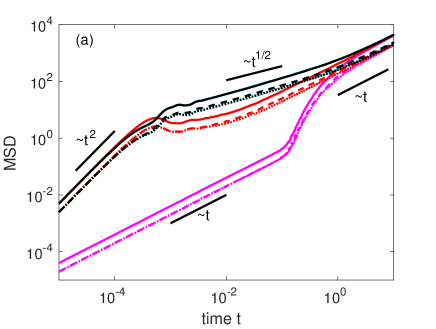
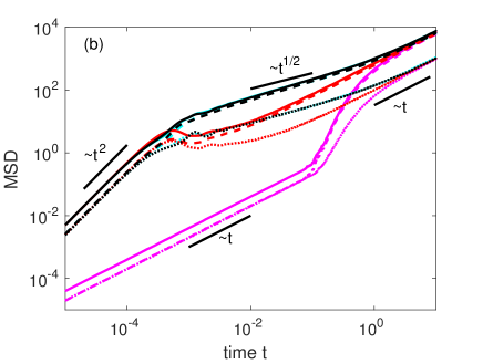
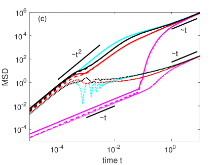
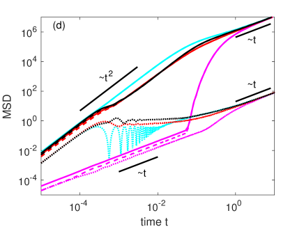
Figure 5: Temporal evolution of MSD for $10^{4}$ walks at $\mathrm{Pe}=10^{4}$. Solid lines: total MSD, dashed lines: MSD parallel to the jet, dotted lines: MSD orthogonal to the jet. Starting positions are denoted by coloring: central streamline of a jet (light cyan), center of an eddy (magenta), flooded (dark red) and the separatrix between jet and eddy (black). Panels: (a) $A=10^{-3}$, (b) $A=10^{-2}$, (c) $A=10^{-1}$, and (d) $A=0.25$. Note that in (a) and (b) the jet region is so thin that the MSD for the first and last initial condition (cyan and black) almost coincide. For (a) the parallel and the perpendicular components of the MSDs are almost equal, and the eddy lattice flow PoeschkeEtAl2016 is being reproduced. Note also that in (d) the MSD for the flooded case (red) and the start on the separatrix (black) are very similar.

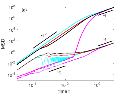
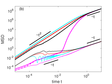
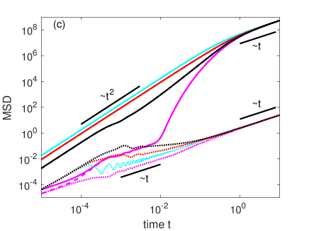
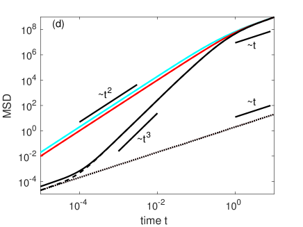
Figure 6: Same as Fig. 5 with (a) $A=0.5$, (b) $A=0.75$, (c) $A=0.9$, and (d) $A=1$. Note that in the flow pattern of (d) there are no eddies, and the corresponding initial condition has converged to the one for a start at the separatrix (black).

IV.3 Aging

For the initial position of tracers at the center of the cat’s eye we also considered the aged MSD: starting at $(x,y)=(\pi/2,\pi/2)$, letting the tracers evolve for the aging time $t_{a}$, and then commencing the observation. Figures 7 and 8 show these aged MSDs. Note that the slopes are the same as in Figs. 5 and 6. The MSDs for other initial conditions are already close to that for the flooded case and thus do age a lot less. Recall that for $A=1$ there are no eddies anymore; their former centers, as well as the former hyperbolic points, lie exactly on the separatrix which, in its turn, becomes a straight line that entirely consists of degenerate stagnation points. For this situation we show in Fig. 8 (d) the process of aging for starting on that straight line.

For $A\neq 1$ the aged MSD as a function of time is oscillating. As shown in PoeschkeEtAl2016 , for sufficiently small $A$ and not too large values of times and aging times $t,t_{a}\ll 1$, the leading terms for the aged MSD are given by

$$\mathrm{MSD}(t,t_{a}) \approx 8(t+t_{a})+\frac{8(t+t_{a})}{\left[1+(2\Omega\,t(t+t_{a}))^{2}\right]^{2}}$$

$$\times\left\{\left[(2\Omega\,t(t+t_{a}))^{2}-1\right]\cos(\Omega\,t)\right.$$

$$\qquad\left.-4\Omega\,t(t+t_{a})\sin(\Omega\,t)\right\},$$

where the frequency of oscillations $\Omega\approx\mathrm{Pe}\,\sqrt{1-A^{2}}$ is a monotonically decreasing function of $A$. For this approximation to work well, the aging time should strongly exceed one period: $t_{a}\gg{2\pi}/{\Omega}$.

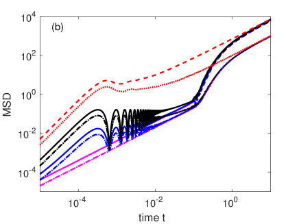
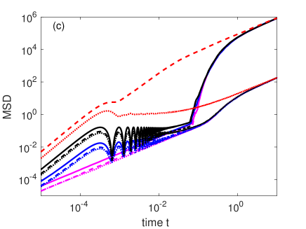
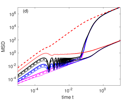
Figure 7: Aged MSD for $10^{4}$ walks starting at the eddy center at $\mathrm{Pe}=10^{4}$. Solid lines: total MSD, dashed lines: MSD parallel to the jet, dotted lines: MSD orthogonal to the jet. Aging times: $t_{a}=0$ (magenta), $t_{a}=10^{-3}$ (blue) and $t_{a}=10^{-2}$ (black). Panels: (a) $A=10^{-3}$, (b) $A=10^{-2}$, (c) $A=10^{-1}$, and (d) $A=0.25$. For $t_{a}\gg t_{2}$ the MSD converges to the flooded case (red dashed) respectively to its orthogonal part (red dotted). In (a) the jet region is so thin, that the eddy lattice flow is reproduced. Here the parallel and the orthogonal components are approximately the same.

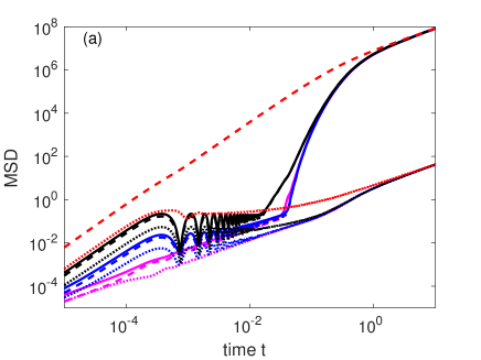
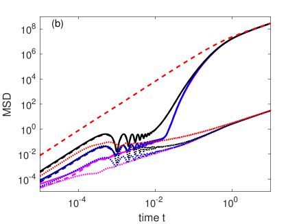
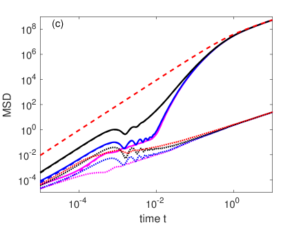
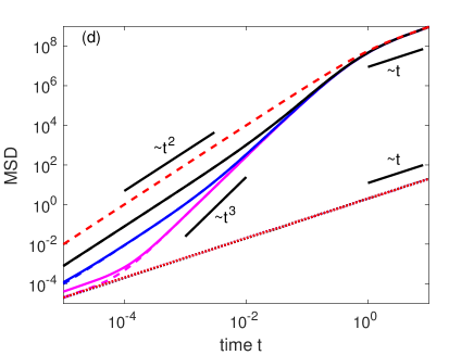
Figure 8: Same as Fig. 7 with (a) $A=0.5$, (b) $A=0.75$, (c) $A=0.9$, and (d) $A=1$. Note that at $A=1$ there are no eddies. Their former centers lie on the straight lines which consist of degenerate equilibria. Here, aging for tracers that start on these lines is shown.

V Conclusions

We considered the advection-diffusion problem for tracer particles in the cat’s eye flow. This two-dimensional flow consists of jet regions having a shape of meandering strips, and eddies having a shape of cat’s eyes. The family of the cat’s eye flows is parametrized by a single parameter, and interpolates between the eddy lattice flow (without jets) and a shear flow with sinusoidal velocity profile (without eddies). In the absence of molecular diffusion, the tracers are either carried away ballistically by jets, or stay trapped in eddies. Adding small thermal noise makes possible the transitions between eddies and jets, and, at long times, leads to anisotropic diffusion with the diffusion coefficient in the jet’s direction much larger than the one in the perpendicular direction. This long time regime seems to be the only one which was discussed theoretically in considerable detail. At intermediate time scales the transport can be modeled by a stochastic scheme corresponding to Lévy walks interrupted by rests. The transport phase of the walk corresponds to the motion in a jet, and rests to trapping in eddies. This scheme however only applies for the initial conditions corresponding to starting close to the separatrix. The behavior for other initial conditions may be vastly different.

In the present work we provide results of extensive numerical simulations of the particles’ transport by the cat’s eye flow concentrating on the mean squared displacement of the particles from their initial positions in a broad time domain, and investigate its intermediate-time behavior, the influence of initial conditions, and aging regimes, i.e. the behavior of MSD between some intermediate time $t_{a}$ and final observation time $t>t_{a}$. The results of simulations confirm theoretical results for the long time behavior of MSD, and the applicability of the Lévy walk scheme for intermediate times, including the prediction about the connection between the transport velocities in the short- and intermediate-time ballistic regimes. They also show a multitude of possible aging behaviors (depending on initial conditions), including an oscillatory one which is observed when particles start inside the eddies. This oscillatory behavior is due to the particles’ rotation in an eddy during the trapping phase, and is not captured by the Lévy walk scheme.

Appendix A Derivation of the intermediate asymptotic MSD

In this section we derive the asymptotic expression for the MSD, Eq. (19), for intermediate times when starting at the separatrix. Since the MSD is dominated by the longitudinal motion along the axis of the system, a one-dimensional model is adequate. We use Lévy walks interrupted by rests as a theoretical description. The derivation follows KlaS .

Let $P_{1}(x,t)$ be the probability density of a tracer being at position $x$ at time $t$ when starting in a ballistic mode and alternating between ballistic motions with velocity $v$ and rests. Given the probability densities of waiting times inside a jet (without index), for resting times (with index $r$) as well as for the last, incomplete step respectively rest (upper-case symbols), we obtain

$$P_{1}(x,t) = \Phi(x,t)+\int_{0}^{t}\phi(x,t^{\prime})\Phi_{r}(t-t^{\prime})\,dt^{\prime}$$

$$+\int_{-\infty}^{\infty}dx^{\prime}\int_{0}^{\infty}dt^{\prime}\int_{0}^{t^{\prime}}dt^{\prime\prime}$$

$$\times\phi(x^{\prime},t^{\prime\prime})\phi_{r}(t-t^{\prime})\Phi(x-x^{\prime},t-t^{\prime})+\dots,$$

respectively

$$P_{1}(k,s) = \Phi(k,s)+\phi(k,s)\Phi_{r}(s)$$

$$+[\phi(k,s)\phi_{r}(s)]^{1}\Phi(k,s)$$

$$+[\phi(k,s)\phi_{r}(s)]^{1}\phi(k,s)\Phi_{r}(s)+\dots$$

$$+[\phi(k,s)\phi_{r}(s)]^{n}\Phi(k,s)$$

$$+[\phi(k,s)\phi_{r}(s)]^{n}\phi(k,s)\Phi_{r}(s)+\dots$$

in Fourier-Laplace representation. By applying the geometric series to odd and even terms separately and averaging the result with the one from an analog calculation for starting in the resting phase, we arrive at

$$P(k,s)=\frac{\Phi(k,s)(1+\phi_{r}(s))+\Phi_{r}(s)(1+\phi(k,s))}{2(1-\phi_{r}(s)\phi(k,s))}$$ (35)

for the probability density of being at time $t$ at position $x$ on the axis Fourier-transformed in space and Laplace-transformed in time. Numerics show that the waiting time densities of a tracer inside a jet respectively a vortex can roughly be approximated by a power law $\propto t^{-3/2}$, if the parameter $A$ is not too small, as expected in theory. Hence we get

$$\phi_{r}(s) = 1-\sqrt{\tau s}$$ (36)

$$\Phi_{r}(s) = \sqrt{\frac{\tau}{s}}$$ (37)

$$\Phi(k,s) = \mathrm{Re}\left\{\sqrt{\frac{\tau}{s+ivk}}\right\}$$

$$= \frac{\sqrt{\tau}\cos\left(\frac{1}{2}\arctan\left(\frac{vk}{s}\right)\right)}{(s^{2}+v^{2}k^{2})^{1/4}}$$

as well as

$$\phi(k,s)=\frac{1}{2}\sqrt{\frac{\tau}{\pi}}\int_{\tau/\pi}^{\infty}t^{-3/2}\cos(kvt)e^{-st}\;dt.$$ (39)

Writing the cosine complex one obtains

$$\phi(k,s) = e^{-\frac{\tau}{\pi}s}\cos\left(\frac{\tau}{\pi}kv\right)$$

$$+\frac{\sqrt{s+ikv}}{2}\left[-\sqrt{\tau}+\mathrm{erf}\left(\sqrt{\frac{\tau}{\pi}(s+ikv)}\right)\right]$$

$$+\frac{\sqrt{s-ikv}}{2}\left[-\sqrt{\tau}+\mathrm{erf}\left(\sqrt{\frac{\tau}{\pi}(s-ikv)}\right)\right].$$

Substituting everything into (35) and expanding both its numerator and its denominator separately first in $k$ until second order and then in $s$ until first order, keeping only the highest order terms in $s$ in each coefficient of the series of $k$ yields

$$P(k,s)=\frac{4\sqrt{\frac{\tau}{s}}-\frac{3\sqrt{\tau}v^{2}}{4s^{5/2}}k^{2}}{4\sqrt{\tau s}+\frac{\sqrt{\tau}v^{2}}{4s^{3/2}}k^{2}}=\frac{1}{s}\frac{\left[1-\frac{3}{16}\left(\frac{vk}{s}\right)^{2}\right]}{\left[1+\frac{1}{16}\left(\frac{vk}{s}\right)^{2}\right]},$$ (41)

i.e.

$$P(k,s)=\frac{1}{s}\left[1-\frac{1}{4}\left(\frac{vk}{s}\right)^{2}\right]$$ (42)

in second order in $k$. From the probability density follows the MSD

$$\mathrm{MSD}(s)=\frac{1}{2}v^{2}s^{-3},$$ (43)

which according to Tauberian theorems for the inverse Laplace-transform corresponds to (19) in real time.

References

- (1) W. Thomson (Lord Kelvin), Nature 23, 45 (1880).
- (2) S. Childress and A. M. Soward, J. Fluid. Mech. 205, 99 (1989).
- (3) A. Fannjiang, J. Diff. Eq. 179, 433 (2002).
- (4) J. P. Bouchaud and A. Georges, Phys. Rep. 195, 127 (1990).
- (5) M. B. Isichenko, Rev. Mod. Phys. 64, 961 (1992).
- (6) W. Young, A. Pumir, and Y. Pomeau, Phys. Fluids A 1, 462 (1989).
- (7) S. Childress, Phys. Earth Planet. Inter. 20, 172 (1979).
- (8) A. M. Soward, J. Fluid Mech. 180, 267 (1987).
- (9) B. I. Shraiman, Phys. Rev. A 36, 261 (1987).
- (10) M. N. Rosenbluth, H. L. Berk, I. Doxas, and W. Horton, Phys. Fluids 30, 2636 (1987).
- (11) A. J. Majda and P. R. Kramer, Phys. Rep. 314, 237 (1999).
- (12) P. Pöschke, I. M. Sokolov, A. A. Nepomnyashchy, and M. A. Zaks, Phys. Rev. E 94, 032128 (2016).
- (13) G. Iyer and A. Novikov, Probab. Theory Relat. Fields 164, 707 doi:10.1007/s00440-015-0617-9 (2016).
- (14) M. Hairer et al., arXiv:1607.01859 [math.PR] (2016).
- (15) A. Fannjiang and G. Papanicolaou, SIAM: J. Appl. Math. 54, 333 (1994).
- (16) T. H. Solomon, E. R. Weeks, and H. L. Swinney, Phys. Rev. Lett. 71, 3975 (1993).
- (17) T. H. Solomon, E. R. Weeks, and H. L. Swinney, Physica D 76, 70 (1994).
- (18) E. R. Weeks, J. S. Urbach, and H. L. Swinney, Physica D 97, 291 (1996).
- (19) V. Zaburdaev, S. Denisov, and J. Klafter, Rev. Mod. Phys. 87, 483 (2015).
- (20) D. Froemberg and E. Barkai, Phys. Rev. E 87, 030104(R), (2013).
- (21) M. Magdziarz and T. Zorawik, Phys. Rev. E 95, 022126 (2017).
- (22) The original flow in Childress1989 was three-dimensional. For our purposes its in-plane components are quite sufficient.
- (23) R. Mannella, in Stochastic processes in physics, chemistry, and biology (Springer, Berlin Heidelberg, 2000), p. 353.
- (24) E. A. Novikov, J. Appl. Math. Mech. 22, 412 (1958).
- (25) R. T. Foister and T. G. M. Van De Ven, J. Fluid Mech. 96, 105 (1980).
- (26) J. Klafter and I. M. Sokolov, First steps in Random Walks (Oxford University Press, Oxford, 2011).