Entropy production of active particles and for particles in active baths

Abstract

Entropy production of an active particle in an external potential is identified through a thermodynamically consistent minimal lattice model that includes the chemical reaction providing the propulsion and ordinary translational noise. In the continuum limit, a unique expression follows, comprising a direct contribution from the active process and an indirect contribution from ordinary diffusive motion. From the corresponding Langevin equation, this physical entropy production cannot be inferred through the conventional, yet here ambiguous, comparison of forward and time-reversed trajectories. Generalizations to several interacting active particles and passive particles in a bath of active ones are presented explicitly, further ones are briefly indicated.

Keywords: active matter, entropy production

Active particles have become a major paradigm of non-equilibrium statistical physics. Endowed with some propulsion mechanism, they perform persistent motion in one direction until the latter changes either due to smooth rotational diffusion or, as in bacteria, due to major reorientation. Already on the single particle level and even more so for many interacting ones, they exhibit a variety of new phenomena, which can be modeled and understood with effective equations of motion as described in several recent reviews [1, 2, 3, 4, 5, 6, 7, 8, 9, 10, 11, 12, 13]. A related class of systems are those where passive particles are put into a bath of such active ones, like colloidal particles in a laser trap that are pushed around by bacteria present in the embedding aqueous solution [14, 15]. On a phenomenological level, the motion of the passive particle in such a non-equilibrium bath [16, 17, 18, 19, 20, 21] can be described in a quite similar way as in the first case.

Several recent works seek to formulate a thermodynamic foundation for the so far phenomenological models of active Brownian particles [22, 23, 24, 25, 26, 27]. In particular, identifying the entropy production necessarily associated with any such non-equilibrium system is a non-trivial problem. One route is to follow stochastic thermodynamics [28] and identify entropy production from comparing the weights for forward and time-reversed trajectories. However, such a procedure depends on the chosen level of coarse-graining and is hence not unique, as recent studies of active Ornstein-Uhlenbeck particles have shown [29, 30, 31, 32]. Similar concepts have been applied in order to identify entropy production for field theories of active matter [33] and for active particles driven in linear response by chemical reactions [34].

In this paper, we identify entropy production for active particles by first starting from a simplified but still thermodynamically consistent lattice model where a chemical reaction leads to propulsion. Earlier lattice models for active particles have not considered this thermodynamic aspect [35, 36, 37]. In addition to this active process, we allow for re-orientations of the director and include ordinary translational diffusion. In the continuum limit of a small step size per reaction event, we find a unique expression for the total entropy production. On the basis of an effective Langevin description of the model, however, two different definitions of entropy production based on the weights of forward and time-reversed trajectories are conceivable. We demonstrate that these differ from the total entropy production and trace this discrepancy to the fact that any such Langevin equation contains implicit coarse-graining as soon as at least two microscopic processes govern the motion like here chemical reactions and the ever-present thermal translational noise.

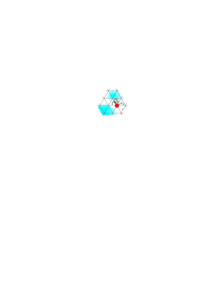
Figure 1: Illustration of the lattice model for an active particle. The particle jumps along the edges of a lattice in a potential landscape. Transitions along the director ${\boldsymbol{n}}$ can be driven by a chemical reaction (indicated by the rates $k^{+}$ and $k^{-}$). Thermal noise induces rotational transitions of the director ${\boldsymbol{n}}$ (rate $\gamma$) and translational transitions in any lattice direction (rate $w$).

We start with a lattice model for an active particle in two dimensions on either a square or a triangular lattice with lattice constant $a$, see Fig. 1. The sites are labeled by ${\boldsymbol{r}}_{i}$ and the four (six) lattice vectors oriented along the adjacent edges of the square (triangular) lattice are labeled by ${\boldsymbol{e}}_{i}$. The active particle has an orientation ${\boldsymbol{n}}$ that is at any time parallel to one of these lattice vectors. Propulsion of the particle one lattice unit in direction ${\boldsymbol{n}}$ arises from a not further specified chemical reaction that liberates a free energy $\Delta\mu$ in each reaction step. This chemical reaction occurs with a rate $k^{+}$ in this forward direction. Thermodynamic consistency requires that the rate $k^{-}$ for the backward reaction with a concomitant step in the $-{\boldsymbol{n}}$ direction to happen obeys the ratio

$$k^{+}/k^{-}=\exp\Delta\mu.$$ (1)

Throughout the paper we set $k_{B}=T=1$, i.e., entropy is dimensionless and all energies are measured in units of the embedding bath temperature. If the orientation ${\boldsymbol{n}}$ of the particle was fixed, the mean velocity $u_{\mathrm{ac}}$ and the dispersion $D_{\rm{ac}}$ of this then effectively one-dimensional motion would be given by

$$u_{\mathrm{ac}}=(k^{+}-k^{-})a~{}~{}~{}\textup{and}~{}~{}~{}D_{\rm{ac}}=(k^{+}+k^{-})a^{2}/2.$$ (2)

It will later be convenient to express the rates in terms of these quantities as

$$k^{\pm}=D_{\rm{ac}}/a^{2}\pm u_{\mathrm{ac}}/2a.$$ (3)

In the presence of an additional potential $V({\boldsymbol{r}}_{i})$, thermodynamic consistency requires that these rates become inhomogeneous. The symmetric choice

$$k^{\pm}({\boldsymbol{r}}_{i},{\boldsymbol{n}})=k^{\pm}\exp[-(V({\boldsymbol{r}}_{i}\pm a{\boldsymbol{n}})-V({\boldsymbol{r}}_{i}))/2]$$ (4)

ensures that the local detailed balance condition

$$k^{+}({\boldsymbol{r}}_{i},{\boldsymbol{n}})/k^{-}({\boldsymbol{r}}_{i}+a{\boldsymbol{n}},{\boldsymbol{n}})=\exp[V({\boldsymbol{r}}_{i})-V({\boldsymbol{r}}_{i}+a{\boldsymbol{n}})+\Delta\mu]$$ (5)

is respected.

In addition to these moves generated by the chemical reaction driving the particle, the orientation ${\boldsymbol{n}}$ becomes stochastic as well. In the simplest case, this orientation undergoes Markovian transitions with a rate $\gamma$ between two adjacent orientations. Under this dynamics, for periodic boundary conditions, or with a confining potential on an infinite plane, the particle reaches a steady state with the probability $p({\boldsymbol{r}}_{i},{\boldsymbol{n}})$ to find it at site ${\boldsymbol{r}}_{i}$ with an orientation ${\boldsymbol{n}}$. The stationary probability current from ${\boldsymbol{r}}_{i}$ in the direction of ${\boldsymbol{n}}$ is then

$$j_{\rm{ac}}({\boldsymbol{r}}_{i},{\boldsymbol{n}})\equiv p({\boldsymbol{r}}_{i},{\boldsymbol{n}})k^{+}({\boldsymbol{r}}_{i},{\boldsymbol{n}})-p({\boldsymbol{r}}_{i}+a{\boldsymbol{n}},{\boldsymbol{n}})k^{-}({\boldsymbol{r}}_{i}+a{\boldsymbol{n}},{\boldsymbol{n}}).$$ (6)

The entropy production rate $\sigma_{{\rm ac}}$ of this active particle in the steady state now follows uniquely from the usual rules of stochastic thermodynamics by summing over all transitions as [38, 28]

$$\sigma_{{\rm ac}}=\sum_{i,{\boldsymbol{n}}}{j_{\rm{ac}}({\boldsymbol{r}}_{i},{\boldsymbol{n}})}\ln[k^{+}({\boldsymbol{r}}_{i},{\boldsymbol{n}})/k^{-}({\boldsymbol{r}}_{i}+a{\boldsymbol{n}},{\boldsymbol{n}})].$$ (7)

There is no explicit contribution from the re-orientational moves of the director ${\boldsymbol{n}}$, since the forward and backward rate for each such link is the same, given by $\gamma$, and hence the corresponding logarithmic term would vanish. This orientational dynamics, however, affects the stationary state, which is, in general, hard to compute but not explicitly required for stating this expression of entropy production due to the active process.

Preparing for a continuum limit, we now assume that the lattice constant $a$ is small compared to the length-scale of variations of the potential and the stationary distribution. We can then expand the rates (4) as

$$k^{\pm}({\boldsymbol{r}}_{i},{\boldsymbol{n}})\approx(D_{\rm{ac}}/a^{2})(1\pm u_{\mathrm{ac}}a/2D_{\rm{ac}})(1\mp a{\boldsymbol{n}}{\boldsymbol{\nabla}}V({\boldsymbol{r}}_{i})/2).$$ (8)

Likewise, the stationary distribution can be expanded as

$$p({\boldsymbol{r}}_{i}+a{\boldsymbol{n}},{\boldsymbol{n}})\approx p({\boldsymbol{r}}_{i},{\boldsymbol{n}})[1+a{\boldsymbol{n}}{\boldsymbol{\nabla}}\ln p({\boldsymbol{r}}_{i},{\boldsymbol{n}})].$$ (9)

Inserting these expansions into (6) and (7) and collecting the terms that dominate in the limit $a\to 0$, one gets

$$j_{\rm{ac}}({\boldsymbol{r}}_{i},{\boldsymbol{n}})=p({\boldsymbol{r}}_{i},{\boldsymbol{n}})[u_{\mathrm{ac}}-D_{\rm{ac}}{\boldsymbol{n}}{\boldsymbol{\nabla}}(V({\boldsymbol{r}}_{i})+\ln p({\boldsymbol{r}}_{i},{\boldsymbol{n}}))]/a$$ (10)

for the magnitude of the corresponding vector-valued current density ${\boldsymbol{j}}_{\rm{ac}}({\boldsymbol{r}}_{i},{\boldsymbol{n}})\equiv{\boldsymbol{n}}j_{\rm{ac}}({\boldsymbol{r}}_{i},{\boldsymbol{n}})$. The entropy production rate becomes

$$\sigma_{{\rm ac}}=\sum_{i,{\boldsymbol{n}}}{j_{\rm{ac}}({\boldsymbol{r}}_{i},{\boldsymbol{n}})}\,a\,[u_{\mathrm{ac}}/D_{\rm{ac}}-{\boldsymbol{n}}{\boldsymbol{\nabla}}V({\boldsymbol{r}}_{i})].$$ (11)

In the continuum limit, we implicitly redefine $p({\boldsymbol{r}},{\boldsymbol{n}})$ and ${\boldsymbol{j}}({\boldsymbol{r}},{\boldsymbol{n}})$ as densities by dividing $p({\boldsymbol{r}}_{i},{\boldsymbol{n}})$ and ${\boldsymbol{j}}({\boldsymbol{r}}_{i},{\boldsymbol{n}})$ by the area of the associated unit cell of the lattice; ${\boldsymbol{j}}({\boldsymbol{r}}_{i},{\boldsymbol{n}})$ obtains the correct dimensionality of a current density by additional multiplication with $a$. Replacing now the summation over ${\boldsymbol{r}}_{i}$ by an integration over ${\boldsymbol{r}}$, we find as our first result that the entropy production rate due to the active process can finally be expressed as

$$\sigma_{{\rm ac}} =\langle(u_{\mathrm{ac}}-D_{\rm{ac}}{\boldsymbol{n}}{\boldsymbol{\nabla}}V({\boldsymbol{r}}))^{2}\rangle/D_{\rm{ac}}-D_{\rm{ac}}\sum_{\boldsymbol{n}}\int d{\boldsymbol{r}}[{\boldsymbol{n}}{\boldsymbol{\nabla}}p({\boldsymbol{r}},{\boldsymbol{n}})][u_{\mathrm{ac}}-{\boldsymbol{n}}{\boldsymbol{\nabla}}V({\boldsymbol{r}})]$$

$$=\langle(u_{\mathrm{ac}}-D_{\rm{ac}}{\boldsymbol{n}}{\boldsymbol{\nabla}}V({\boldsymbol{r}}))^{2}\rangle/D_{\rm{ac}}-D_{\rm{ac}}\langle({\boldsymbol{n}}{\boldsymbol{\nabla}})^{2}V({\boldsymbol{r}})\rangle,$$ (12)

where we have applied integration by parts to the second term. Here, and in the following, the angular brackets $\langle...\rangle$ denote an average in the stationary state $p({\boldsymbol{r}},{\boldsymbol{n}})$.

So far, we have not yet included ordinary thermal translational diffusion. We can do so by allowing additional moves from ${\boldsymbol{r}}_{i}$ to ${\boldsymbol{r}}_{i}+a{\boldsymbol{e}}_{i}$ with a rate

$$w({\boldsymbol{r}}_{i},{\boldsymbol{e}}_{i})=w\exp[-(V({\boldsymbol{r}}_{i}+a{\boldsymbol{e}}_{i})-V({\boldsymbol{r}}_{i}))/2],$$ (13)

where $w\equiv D_{\rm{tr}}a^{2}$ is the bare discrete jump rate and $D_{\rm{tr}}$ the diffusion constant on a square lattice. For a triangular lattice, one has to choose $w=2D_{\rm{tr}}/3a^{2}$. The corresponding probability current from ${\boldsymbol{r}}_{i}$ in the direction ${\boldsymbol{e}}_{i}$ is then

$$j_{\rm{tr}}({\boldsymbol{r}}_{i},{\boldsymbol{n}},{\boldsymbol{e}}_{i})=p({\boldsymbol{r}}_{i},{\boldsymbol{n}})w({\boldsymbol{r}}_{i},{\boldsymbol{e}}_{i})-p({\boldsymbol{r}}_{i}+a{\boldsymbol{e}}_{i},{\boldsymbol{n}})w({\boldsymbol{r}}_{i},-{\boldsymbol{e}}_{i}).$$ (14)

Going through the same steps as above, for both lattices, one gets the current density

$${\boldsymbol{j}}_{\rm{tr}}({\boldsymbol{r}}_{i},{\boldsymbol{n}})=-D_{\rm{tr}}p({\boldsymbol{r}}_{i},{\boldsymbol{n}}){\boldsymbol{\nabla}}[V({\boldsymbol{r}}_{i})+\ln p({\boldsymbol{r}}_{i},{\boldsymbol{n}})]$$ (15)

and the entropy production rate due to the translational diffusive steps

$$\sigma_{{\rm tr}}=-\sum_{\boldsymbol{n}}\int d{\boldsymbol{r}}\,{\boldsymbol{j}}_{\rm{tr}}({\boldsymbol{r}},{\boldsymbol{n}}){\boldsymbol{\nabla}}V({\boldsymbol{r}})=D_{\rm{tr}}\langle[{\boldsymbol{\nabla}}V({\boldsymbol{r}})]^{2}-{\boldsymbol{\nabla}}^{2}V({\boldsymbol{r}})\rangle,$$ (16)

which is, in the first form, well-known from ordinary stochastic thermodynamics as the entropy production in the medium [28, Sec. 2.5], which is in the steady state equal to the total entropy production, and the second equality follows with an integration by parts. In equilibrium, i.e., without an active process, $\sigma_{{\rm tr}}$ vanishes since for a Boltzmann distribution $\sim\exp[-V({\boldsymbol{r}}_{i})]$ the two terms above cancel. For an active process, the stationary distribution is no longer of this form and, hence, in the presence of a potential even these translational diffusive steps can contribute to the entropy production rate, which is our second main insight. The total entropy production rate becomes

$$\sigma_{\rm{tot}} \equiv\sigma_{{\rm ac}}+\sigma_{{\rm tr}}$$

$$=\langle(u_{\mathrm{ac}}-D_{\rm{ac}}{\boldsymbol{n}}{\boldsymbol{\nabla}}V({\boldsymbol{r}}))^{2}\rangle/D_{\rm{ac}}-D_{\rm{ac}}\langle({\boldsymbol{n}}{\boldsymbol{\nabla}})^{2}V({\boldsymbol{r}})\rangle+D_{\rm{tr}}\langle[{\boldsymbol{\nabla}}V({\boldsymbol{r}})]^{2}-{\boldsymbol{\nabla}}^{2}V({\boldsymbol{r}})\rangle.$$ (17)

Since this result no longer contains any explicit reference to the originally underlying lattice, it should be obvious that it holds as a continuum result also for three-dimensional active motion. Moreover, it holds for any non-driven Markovian dynamics of the orientation ${\boldsymbol{n}}$ as long as the latter is independent of the spatial position. Therefore, it includes ordinary active Brownian particles with their orientational diffusion [3].

The stationary distribution underlying above averages follows in the discrete case from the stationary master equation, which we cast in the shape of a balance equation for the edge currents (6) and (14)

$$0=\partial_{t}p({\boldsymbol{r}}_{i},{\boldsymbol{n}})=j_{\rm{ac}}({\boldsymbol{r}}_{i}-a{\boldsymbol{n}},{\boldsymbol{n}})-j_{\rm{ac}}({\boldsymbol{r}}_{i},{\boldsymbol{n}})-\sum_{{\boldsymbol{e}}_{i}}j_{\rm{tr}}({\boldsymbol{r}}_{i},{\boldsymbol{n}},{\boldsymbol{e}}_{i})+L_{\boldsymbol{n}}p({\boldsymbol{r}}_{i},{\boldsymbol{n}}),$$ (18)

where the operator $L_{{\boldsymbol{n}}}$ acting solely on ${\boldsymbol{n}}$ conveys the non-driven dynamics of the rotational degree of freedom. Likewise in the continuum limit, the stationary distribution is the solution of the stationary Fokker-Planck equation that follows from the continuity of the currents (10) and (15) as

$$0=\partial_{t}p({\boldsymbol{r}},{\boldsymbol{n}}) =-{\boldsymbol{\nabla}}[{\boldsymbol{j}}_{\rm{ac}}({\boldsymbol{r}},{\boldsymbol{n}})+{\boldsymbol{j}}_{\rm{tr}}({\boldsymbol{r}},{\boldsymbol{n}})]+L_{{\boldsymbol{n}}}p({\boldsymbol{r}},{\boldsymbol{n}})$$

$$=-{\boldsymbol{\nabla}}{\boldsymbol{n}}[u_{\mathrm{ac}}-D_{\rm{ac}}{\boldsymbol{n}}({\boldsymbol{\nabla}}V({\boldsymbol{r}}))]p({\boldsymbol{r}},{\boldsymbol{n}})+D_{\rm{ac}}({\boldsymbol{n}}{\boldsymbol{\nabla}})^{2}p({\boldsymbol{r}},{\boldsymbol{n}})$$

$$\qquad+D_{\rm{tr}}{\boldsymbol{\nabla}}[({\boldsymbol{\nabla}}V({\boldsymbol{r}}))p({\boldsymbol{r}},{\boldsymbol{n}})]+D_{\rm{tr}}{\boldsymbol{\nabla}}^{2}p({\boldsymbol{r}},{\boldsymbol{n}})+L_{{\boldsymbol{n}}}p({\boldsymbol{r}},{\boldsymbol{n}}).$$ (19)

For a continuous space of orientations ${\boldsymbol{n}}$, the operator $L_{\boldsymbol{n}}$ becomes the Fokker-Planck operator governing the stochastic dynamics of ${\boldsymbol{n}}$. For example, in two dimensions, for a dipolar interaction through the potential $\mathcal{U}({\boldsymbol{n}})=-{\boldsymbol{B}}{\boldsymbol{n}}$ , this operator would read $L_{\boldsymbol{n}}\propto\partial_{\theta}^{2}+B\partial_{\theta}\sin\theta$, where $\theta$ denotes the angle between ${\boldsymbol{n}}$ and the homogeneous field ${\boldsymbol{B}}$. Multiplication of equation (Entropy production of active particles and for particles in active baths) by $V({\boldsymbol{r}})$ and repeated integration by parts leads to the relation

$$0=\left\langle{\boldsymbol{n}}{\boldsymbol{\nabla}}V({\boldsymbol{r}})[u_{\mathrm{ac}}-D_{\rm{ac}}{\boldsymbol{n}}{\boldsymbol{\nabla}}V({\boldsymbol{r}})]\right\rangle+D_{\rm{ac}}\left\langle({\boldsymbol{n}}{\boldsymbol{\nabla}})^{2}V({\boldsymbol{r}})\right\rangle-D_{\rm{tr}}\left\langle[{\boldsymbol{\nabla}}V({\boldsymbol{r}})]^{2}\right\rangle+D_{\rm{tr}}\left\langle{\boldsymbol{\nabla}}^{2}V({\boldsymbol{r}})\right\rangle,$$ (20)

which can be used to write the expression (12) for the active part of the entropy production as

$$\sigma_{{\rm ac}}=u_{\mathrm{ac}}^{2}/D_{\rm{ac}}-u_{\mathrm{ac}}\left\langle{\boldsymbol{n}}{\boldsymbol{\nabla}}V({\boldsymbol{r}})\right\rangle-D_{\rm{tr}}\left\langle[{\boldsymbol{\nabla}}V({\boldsymbol{r}})]^{2}\right\rangle+D_{\rm{tr}}\left\langle{\boldsymbol{\nabla}}^{2}V({\boldsymbol{r}})\right\rangle.$$ (21)

Consequently, the total entropy production (17) becomes

$$\sigma_{\rm{tot}}=u_{\mathrm{ac}}^{2}/D_{\rm{ac}}-u_{\mathrm{ac}}\left\langle{\boldsymbol{n}}{\boldsymbol{\nabla}}V({\boldsymbol{r}})\right\rangle.$$ (22)

For a comparison with previous work, we state for our model on the continuum level the corresponding Langevin dynamics, which can be read off from the Fokker-Planck equation (Entropy production of active particles and for particles in active baths) as

$$\dot{{\boldsymbol{r}}}=u_{\mathrm{ac}}{\boldsymbol{n}}-(D_{\rm{tr}}+D_{\rm{ac}}{\boldsymbol{n}}\otimes{\boldsymbol{n}}){\boldsymbol{\nabla}}V({\boldsymbol{r}})+{\boldsymbol{\zeta}}_{\rm{tr}}+\zeta_{\rm{ac}}{\boldsymbol{n}}.$$ (23)

It contains ordinary thermal translational noise with the correlations

$$\langle{\boldsymbol{\zeta}}_{\rm{tr}}(t_{2})\otimes{\boldsymbol{\zeta}}_{\rm{tr}}(t_{1})\rangle=2D_{\rm{tr}}\boldsymbol{1}\delta(t_{2}-t_{1}).$$ (24)

The chemical driving leads to an active noise, which acts along ${\boldsymbol{n}}$, has correlations

$$\langle\zeta_{\rm{ac}}(t_{2})\zeta_{\rm{ac}}(t_{1})\rangle=2D_{\rm{ac}}\delta(t_{2}-t_{1}),$$ (25)

and is uncorrelated with the translational noise. Thermodynamic consistency thus leads to an active “mobility” $D_{\rm{ac}}{\boldsymbol{n}}\otimes{\boldsymbol{n}}$ for motion in a potential, which is reminiscent of the coupling described in Ref. [34] in linear response.

There is no need to specify the orientational dynamics for ${\boldsymbol{n}}(t)$ explicitly, provided it is Markovian, independent of ${\boldsymbol{r}}$, and non-driven. Under these conditions, the stationary distribution factorizes $p({\boldsymbol{r}},{\boldsymbol{n}})=p({\boldsymbol{r}}|{\boldsymbol{n}})p({\boldsymbol{n}})$ with

$$p({\boldsymbol{n}})\sim\exp[-\mathcal{U}({\boldsymbol{n}})],$$ (26)

where the potential $\mathcal{U}({\boldsymbol{n}})$ is constant for ordinary rotational diffusion and $\mathcal{U}({\boldsymbol{n}})=-{\boldsymbol{B}}{\boldsymbol{n}}$ if the director is subject to a dipolar interaction with a field ${\boldsymbol{B}}$.

It might look tempting to infer the entropy production directly from the Langevin equation (23) by comparing the weight of a forward trajectory ${\boldsymbol{r}}(t),{\boldsymbol{n}}(t)$ (for $0\leq t\leq\mathcal{T}$) with that of the corresponding backward trajectory $\tilde{\boldsymbol{r}}(t)={\boldsymbol{r}}(\mathcal{T}-t),\tilde{\boldsymbol{n}}(t)={\boldsymbol{n}}(\mathcal{T}-t)$ [39, 28]. This apparently innocent procedure fails in the presence of two noise sources as the following simple example of free active motion shows. The Langevin equation

$$\dot{{\boldsymbol{r}}}=u_{\mathrm{ac}}{\boldsymbol{n}}+{\boldsymbol{\zeta}}_{\rm{tr}}+\zeta_{\rm{ac}}{\boldsymbol{n}}$$ (27)

with the above given noise correlations leads to the weight (conditioned on the ${\boldsymbol{n}}$-trajectory)

$$p[{\boldsymbol{r}}(t)|{\boldsymbol{n}}(t)]\sim\exp\int_{0}^{\mathcal{T}}dt\bigg{\{}-\frac{(\dot{{\boldsymbol{r}}}{\boldsymbol{n}}-u_{\mathrm{ac}})^{2}}{4D_{||}}-\frac{[(\boldsymbol{1}-{\boldsymbol{n}}\otimes{\boldsymbol{n}})\dot{{\boldsymbol{r}}}]^{2}}{4D_{\rm{tr}}}\bigg{\}},$$ (28)

which follows from the path weights of the components of the white noise (24, 25) in the directions parallel and perpendicular to ${\boldsymbol{n}}$. For the former, the diffusion coefficients for the active and the translational noise add up to $D_{||}\equiv D_{\rm{tr}}+D_{\rm{ac}}$. The part of the exponent that is asymmetric under time reversal becomes after averaging

$$\varSigma\equiv\left\langle\ln\frac{p[{\boldsymbol{r}}(t)|{\boldsymbol{n}}(t)]}{p[\tilde{{\boldsymbol{r}}}(t)|\tilde{{\boldsymbol{n}}}(t)]}\right\rangle/\mathcal{T}=u_{\mathrm{ac}}^{2}/(D_{\rm{tr}}+D_{\rm{ac}})\leq\sigma_{\rm{tot}}=u_{\mathrm{ac}}^{2}/D_{\rm{ac}},$$ (29)

which is less than what we have identified above as physical entropy production rate $\sigma_{\rm{tot}}$. This conventional procedure fails in this case since the trajectory no longer contains the full thermodynamically relevant information. An increment along the ${\boldsymbol{n}}$-direction could be either due to thermal translational noise (without concomitant entropy production in the absence of a potential) or due to an active chemical reaction which comes with entropy production. A comparison on the level of forward and backward trajectories thus implicitly involves some coarse-graining of the underlying microscopic processes in which case the true entropy production is underestimated by a bona-fide comparison of the weights [40, 41, 42, 43, 44, 45].

The inequality $0\leq\varSigma\leq\sigma_{\rm{tot}}$ holds even in the presence of the potential $V({\boldsymbol{r}})$, as we now show. The conditioned path weights corresponding to the Langevin equation (23) read

$$p[{\boldsymbol{r}}(t)|{\boldsymbol{n}}(t)]\sim\exp\int_{0}^{\mathcal{T}}dt\bigg{\{} -\frac{[\dot{{\boldsymbol{r}}}{\boldsymbol{n}}-u_{\mathrm{ac}}+D_{||}{\boldsymbol{n}}{\boldsymbol{\nabla}}V({\boldsymbol{r}})]^{2}}{4D_{||}}-\frac{[(\boldsymbol{1}-{\boldsymbol{n}}\otimes{\boldsymbol{n}})(\dot{{\boldsymbol{r}}}+D_{\rm{tr}}{\boldsymbol{\nabla}}V({\boldsymbol{r}}))]^{2}}{4D_{\rm{tr}}}$$

$$+\frac{D_{||}}{2}({\boldsymbol{n}}{\boldsymbol{\nabla}})^{2}V({\boldsymbol{r}})+\frac{D_{\rm{tr}}}{2}[(\boldsymbol{1}-{\boldsymbol{n}}\otimes{\boldsymbol{n}}){\boldsymbol{\nabla}}]^{2}V({\boldsymbol{r}})\bigg{\}},$$ (30)

where the terms in the second line arise from the Stratonovich discretization rule. With this expression, the quantity $\varSigma$ follows as

$$\varSigma \equiv\left\langle\ln\frac{p[{\boldsymbol{r}}(t)|{\boldsymbol{n}}(t)]}{p[\tilde{{\boldsymbol{r}}}(t)|\tilde{\boldsymbol{n}}(t)]}\right\rangle/\mathcal{T}$$

$$=\left\langle(\dot{{\boldsymbol{r}}}{\boldsymbol{n}})u_{\mathrm{ac}}/D_{||}-\dot{{\boldsymbol{r}}}{\boldsymbol{\nabla}}V({\boldsymbol{r}})\right\rangle=u_{\mathrm{ac}}\left\langle\dot{{\boldsymbol{r}}}{\boldsymbol{n}}\right\rangle/D_{||}=u_{\mathrm{ac}}^{2}/D_{||}-u_{\mathrm{ac}}\left\langle{\boldsymbol{n}}{\boldsymbol{\nabla}}V({\boldsymbol{r}})\right\rangle.$$ (31)

Here, we use that the average $\left\langle\dot{{\boldsymbol{r}}}{\boldsymbol{\nabla}}V({\boldsymbol{r}})\right\rangle$ vanishes, since it is the total differential of $V({\boldsymbol{r}})$, and evaluate the average $\left\langle\dot{{\boldsymbol{r}}}{\boldsymbol{n}}\right\rangle$ via integration by parts from $\int d{\boldsymbol{r}}d{\boldsymbol{n}}{\boldsymbol{j}}({\boldsymbol{r}},{\boldsymbol{n}}){\boldsymbol{n}}$ with the steady state current

$${\boldsymbol{j}}({\boldsymbol{r}},{\boldsymbol{n}})\equiv[D_{\rm{ac}}{\boldsymbol{n}}(u_{\mathrm{ac}}/D_{\rm{ac}}-{\boldsymbol{n}}({\boldsymbol{\nabla}}V({\boldsymbol{r}})))-D_{\rm{ac}}{\boldsymbol{n}}({\boldsymbol{n}}{\boldsymbol{\nabla}})-D_{\rm{tr}}({\boldsymbol{\nabla}}V({\boldsymbol{r}}))-D_{\rm{tr}}{\boldsymbol{\nabla}}]p({\boldsymbol{r}},{\boldsymbol{n}}).$$ (32)

In the fictitious, dynamically equivalent, process for which active and translational diffusion in ${\boldsymbol{n}}$-direction are attributed to the same source of noise, $\varSigma$ would correspond to the true thermodynamic entropy production and therefore $\varSigma\geq 0$. On the other hand, the positivity of $D_{\rm{tr}}$ directly shows that $\varSigma\leq\sigma_{\rm{tot}}$ in the comparison of Eq. (31) with (22). Equality, $\varSigma=\sigma_{\rm{tot}}$, is reached only in the limit of vanishing translational noise [32], i.e., for $D_{\rm{tr}}\to 0$.

For models of active particles that lack both ordinary and active translational diffusion, the full trajectory of the system is described by ${\boldsymbol{r}}(t)$ whereas the director ${\boldsymbol{n}}$ becomes a dependent variable. The time reversal used in Ref. [29] to define an entropy production rate therefore involves, in the simple case of a free particle, the implicit reversal of the director ${\boldsymbol{n}}$. Inspired by this definition, we now consider for the present model a ratio of path weights where this reversal is made explicit, leading to the quantity

$$\varSigma^{\prime}\equiv\left\langle\ln\frac{p[{\boldsymbol{r}}(t)|{\boldsymbol{n}}(t)]}{p[\tilde{{\boldsymbol{r}}}(t)|-\tilde{\boldsymbol{n}}(t)]}\right\rangle/\mathcal{T}=u_{\mathrm{ac}}\left\langle{\boldsymbol{n}}{\boldsymbol{\nabla}}V({\boldsymbol{r}})\right\rangle,$$ (33)

which is zero for a vanishing potential, as is also the case for the entropy production defined in Ref. [29]. Interestingly, this quantity adds up with $\varSigma$ to the potential-independent constant

$$\varSigma+\varSigma^{\prime}=u_{\mathrm{ac}}^{2}/D_{||}$$ (34)

and likewise with the total entropy production to $\sigma_{\rm{tot}}+\varSigma^{\prime}=u_{\mathrm{ac}}^{2}/D_{\rm{ac}}$ . If the dynamics of the director ${\boldsymbol{n}}$ is symmetric under flipping ${\boldsymbol{n}}\mapsto-{\boldsymbol{n}}$, i.e., $p[-{\boldsymbol{n}}(t)]=p[{\boldsymbol{n}}(t)]$, and non-driven, the quantity $\varSigma^{\prime}$ satisfies $0\leq\varSigma^{\prime}\leq u_{\mathrm{ac}}^{2}/D_{||}$, due to the positivity of $\varSigma$ and Jensen’s inequality in

$$\varSigma^{\prime}=-\left\langle\ln\frac{p[\tilde{{\boldsymbol{r}}}(t),-\tilde{\boldsymbol{n}}(t)]}{p[{\boldsymbol{r}}(t),{\boldsymbol{n}}(t)]}\right\rangle/\mathcal{T}\geq-\ln\left\langle\frac{p[\tilde{{\boldsymbol{r}}}(t),-\tilde{\boldsymbol{n}}(t)]}{p[{\boldsymbol{r}}(t),{\boldsymbol{n}}(t)]}\right\rangle/\mathcal{T}=0.$$ (35)

In spite of this positivity, $\varSigma^{\prime}$ does not qualify as a characterization of the physical entropy production, since its dependence on a potential (for fixed $u_{\mathrm{ac}}$ and $D_{\rm{ac}}$) is complementary to the physical dissipation (i.e., to $\sigma_{\rm{tot}}$). The distinction between $\varSigma$ and $\varSigma^{\prime}$ is reminiscent of a similar alternative in the case of external flow [46], see also [27].

The “sum-rule” (34), however, applies only on the continuum level. In the discrete model, the contribution to the logarithmic ratio of path weights (33) from transitions amounts to only the respective changes $\Delta V$ of the potential, since the contribution $\Delta\mu$ from the chemical reaction cancels for inverted ${\boldsymbol{n}}$ in the backward path. Since the change of the potential is zero on average, the only contribution to $\varSigma^{\prime}$ stems from the sojourn times in states where the exit rates for forward and backward path do not cancel, leading to

$$\varSigma^{\prime}=\sum_{i,{\boldsymbol{n}}}p({\boldsymbol{r}}_{i},{\boldsymbol{n}})[-k^{+}({\boldsymbol{r}}_{i},{\boldsymbol{n}})-k^{-}({\boldsymbol{r}}_{i},{\boldsymbol{n}})+k^{+}({\boldsymbol{r}}_{i},-{\boldsymbol{n}})+k^{-}({\boldsymbol{r}}_{i},-{\boldsymbol{n}})],$$ (36)

with no obvious relation to $\varSigma$ or $\sigma_{\rm{tot}}$.

So far, we have dealt with one active particle. Our approach is easily generalized to $N$ interacting particles with positions ${\boldsymbol{r}}^{j}$ and orientation ${\boldsymbol{n}}^{j}$ leading to

$$\sigma_{{\rm ac}}=\sum_{j=1}^{N}\left\{\langle(u_{\mathrm{ac}}-D_{\rm{ac}}{\boldsymbol{n}}^{j}{\boldsymbol{\nabla}}^{j}V(\{{\boldsymbol{r}}^{j}\}))^{2}\rangle/D_{\rm{ac}}-D_{\rm{ac}}\langle({\boldsymbol{n}}^{j}{\boldsymbol{\nabla}}^{j})^{2}V(\{{\boldsymbol{r}}^{j}\})\rangle\right\},$$ (37)

where $V(\{{\boldsymbol{r}}^{j}\})$ comprises the two-body interaction potential and a possible external one-body potential and ${\boldsymbol{\nabla}}^{j}\equiv{\boldsymbol{\nabla}}_{{\boldsymbol{r}}^{j}}$. The diffusive translational contribution $\sigma_{{\rm tr}}$ (16) is likewise additive in the $N$ particles.

This formalism can also easily be applied to $M$ passive colloidal particles ($j=N+1,\dots,N+M$) in a non-equilibrium bath of $N$ active ones ($j=1,...,N$) leading to

$$\sigma_{\rm{tot}} =\sum_{j=1}^{N}\left\{\langle(u_{\mathrm{ac}}-D_{\rm{ac}}{\boldsymbol{n}}^{j}{\boldsymbol{\nabla}}^{j}V(\{{\boldsymbol{r}}^{j}\}))^{2}\rangle/D_{\rm{ac}}-D_{\rm{ac}}\langle({\boldsymbol{n}}^{j}{\boldsymbol{\nabla}}^{j})^{2}V(\{{\boldsymbol{r}}^{j}\})\rangle\right\}$$

$$\qquad+\sum_{j=1}^{M+N}\left\{\langle D_{\rm{tr}}^{j}{\boldsymbol{\nabla}}^{j}V(\{{\boldsymbol{r}}^{j}\})^{2}\rangle-D_{\rm{tr}}^{j}\langle({\boldsymbol{\nabla}}^{j})^{2}V(\{{\boldsymbol{r}}^{j}\})\rangle\right\}$$

$$=Nu_{\mathrm{ac}}^{2}/D_{\rm{ac}}-u_{\mathrm{ac}}\sum_{j=1}^{N}\left\langle{\boldsymbol{n}}^{j}{\boldsymbol{\nabla}}^{j}V(\{{\boldsymbol{r}}^{j}\})\right\rangle,$$ (38)

where $V(\{{\boldsymbol{r}}_{i}\})$ includes all two-body interactions and the external potential.

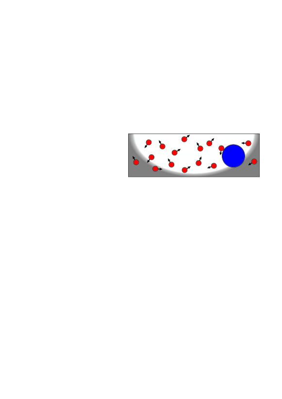
Figure 2: Illustration of a passive particle (blue) interacting via hard-core repulsion with many active particles (red). An external harmonic potential (indicated in gray) acts only one the passive particle.

For a simple example, assume that an external harmonic potential of strength $k$ acts only on one passive colloid embedded in a bath of active ones, see Fig. 2, as realized in experiments [14, 15]. All particles (passive and active ones) are hard-core repulsive. From the first equality in (38), the total entropy production then becomes

$$\sigma_{\rm{tot}}=\rho Nu_{\mathrm{ac}}^{2}/D_{\rm{ac}}+D_{\rm{tr}}k(k\langle{\boldsymbol{r}}^{2}\rangle-d)$$ (39)

in $d$ dimensions and with ${\boldsymbol{r}}$ denoting the position of the passive colloid. On the lattice level, one has to correct for the fact that the reaction step is possible only if the neighboring lattice site is unoccupied which happens for a fraction $\rho<1$ of total phase space that is, in general, not easily computable. The second term is essentially the net heat dissipated through the viscous friction of the passive particle while sliding down diffusively the potential after having been pushed upwards by the active particles.

Building on the minimal thermodynamically consistent model for active particles presented above, several generalizations towards more detailed models are straightforwardly conceivable. First, for non-spherical particles, the translational diffusion tensor will typically not be isotropic. For rod-like particles oriented along ${\boldsymbol{n}}$, one would replace $D_{\rm{tr}}$ by a diffusion tensor of the form

$$\mathbf{D}_{\mathrm{tr}}=D_{\rm{tr}}^{||}{\boldsymbol{n}}\otimes{\boldsymbol{n}}+D_{\rm{tr}}^{\perp}(\boldsymbol{1}-{\boldsymbol{n}}\otimes{\boldsymbol{n}})$$ (40)

with a perpendicular component $D_{\rm{tr}}^{\perp}$ and a parallel component $D_{\rm{tr}}^{||}$. The latter is then relevant in expressions containing $D_{\rm{ac}}+D_{\rm{tr}}$. Second, one could allow for different reaction channels indexed by $\rho$, each with a different $u_{\mathrm{ac}}^{\rho}$ and $D_{\rm{ac}}^{\rho}$ and then sum over the $\rho$.

Third, one can add further internal degrees of freedom to the model, which act as a memory and affect the preferred chemical reaction channel [47]. Formally, if these internal degrees of freedom satisfy a non-driven Markovian dynamics, they can be treated analogously to the degree of freedom associated with ${\boldsymbol{n}}$. In particular, this generalization allows one to emulate the dynamics of active Ornstein-Uhlenbeck particles using one continuous internal degree of freedom $f$, which couples to the propulsion speed as $u_{\mathrm{ac}}\propto f$ and whose dynamics is such that $f{\boldsymbol{n}}$ describes an Ornstein-Uhlenbeck process.

Fourth, one could replace the simple Poisson process used above for modeling the chemical reaction by a more elaborate chemical reaction network, in which each transition comes either with a reaction step or with a displacement step. Such a network would typically be multicyclic, allowing for a weak coupling between the chemical reaction and the stepping of the particle. In a linear response description of the network currents [48], this coupling would be expressed by a small Onsager coefficient [34].

Popular models of active Brownian particles, for example the active Ornstein-Uhlenbeck particles considered in Refs. [29, 30], neglect both active and thermal translational noise in the Langevin equation (23). In our model, setting ${\boldsymbol{\zeta}}_{\rm{tr}}=0$ is thermodynamically consistent. In that case, the entropy production $\varSigma$ in the effective model becomes equal to the total entropy production $\sigma_{\rm{tot}}$. In contrast, setting $\zeta_{\rm{ac}}=0$ breaks micro-reversibility, leading to trajectories that lack a time-reversed counterpart. Thus, in the limit $D_{\rm{ac}}\to 0$ with fixed $u_{\mathrm{ac}}$, the total entropy production $\sigma_{\rm{tot}}$ diverges. Likewise, in the presence of a potential scaling like $V\sim 1/D_{\rm{ac}}$ and for $D_{\rm{tr}}=0$, both $\varSigma$ and $\varSigma^{\prime}$ diverge. Nonetheless, the Langevin equation (23) with ${\boldsymbol{\zeta}}_{\rm{tr}}=\zeta_{\rm{ac}}=0$ may be a valid effective description of large active particles with strong propulsion force. The well-defined stationary distribution for this process can then be used for the averages in Eq. (17) or (38) to obtain the leading order contribution to $\sigma_{\rm{tot}}$ for small but non-zero $D_{\rm{ac}}$. The non-divergent entropies considered for active Ornstein-Uhlenbeck particles in Refs. [29, 30] differ from $\sigma_{\rm{tot}}$, $\varSigma$, and $\varSigma^{\prime}$ and rely on the variability of the propulsion speed $u_{\mathrm{ac}}$ in order to make the coarse-grained trajectories ${\boldsymbol{r}}(t)$ reversible. In models with constant $u_{\mathrm{ac}}$, as considered here, such a definition would not be feasible, let alone lead to the thermodynamic entropy production characterizing the dissipation in the surrounding medium.

In summary, we have determined entropy production for a large class of active particles starting with a thermodynamically consistent lattice model. Its continuum limit offers an alternative to attempts of defining entropy production from path weights from an effective Langevin equation. These definitions underestimate the total entropy production (whenever translational noise cannot be ignored) and suffer from a certain arbitrariness when defining the “time-reversed” path. We have focused on the stationary state and the average entropy production. Extensions to relaxation from an arbitrary initial state or to time-dependent potentials should be straightforward. Likewise, starting with the lattice model, trajectory-dependent entropy production and the corresponding integral and detailed fluctuation theorems can be derived as in ordinary stochastic thermodynamics [28]. Finally, it will be interesting, and presumably somewhat more challenging, to extend this approach to hydrodynamic and field-theoretic descriptions of active particles, and, more generally, of active matter [49, 33, 12, 50].

References

References

- [1] S. Ramaswamy, “The mechanics and statistics of active matter”, Ann. Rev. Cond. Mat. Phys. 1, 323 (2010).
- [2] M. E. Cates, “Diffusive transport without detailed balance in motile bacteria: does microbiology need statistical physics?”, Rep. Prog. Phys. 75, 042601 (2012).
- [3] P. Romanczuk, M. Bär, W. Ebeling, B. Lindner, and L. Schimansky-Geier, “Active Brownian particles”, Eur. Phys. J. Spec. Top. 202, 1 (2012).
- [4] M. C. Marchetti, J. F. Joanny, S. Ramaswamy, T. B. Liverpool, J. Prost, M. Rao, and R. A. Simha, “Hydrodynamics of soft active matter”, Rev. Mod. Phys. 85, 1143 (2013).
- [5] J. Elgeti, R. G. Winkler, and G. Gompper, “Physics of microswimmers – single particle motion and collective behavior: a review”, Rep. Prog. Phys. 78, 056601 (2015).
- [6] M. E. Cates and J. Tailleur, “Motility-induced phase separation”, Ann. Rev. Cond. Mat. Phys. 6, 219 (2015).
- [7] J. Bialké, T. Speck, and H. Löwen, “Active colloidal suspensions: Clustering and phase behavior”, J. Non-Cryst. Solids 407, 367 (2015).
- [8] J. Prost, F. Jülicher, and J.-F. Joanny, “Active gel physics”, Nature Phys. 11, 111 (2015).
- [9] C. Bechinger, R. Di Leonardo, H. Löwen, C. Reichhardt, G. Volpe, and G. Volpe, “Active particles in complex and crowded environments”, Rev. Mod. Phys. 88, 045006 (2016).
- [10] H. Stark, “Swimming in external fields”, Eur. Phys. J. Spec. Top. 225, 2369 (2016).
- [11] G. Oshanin, M. N. Popescu, and S. Dietrich, “Active colloids in the context of chemical kinetics”, J. Phys. A: Math. Theor. 50, 134001 (2017).
- [12] P. Illien, R. Golestanian, and A. Sen, “‘Fuelled’ motion: phoretic motility and collective behaviour of active colloids”, Chem. Soc. Rev. 46, 5508 (2017).
- [13] S. Ramaswamy, “Active matter”, J. Stat. Mech.: Theor. Exp. 2017, 054002 (2017).
- [14] S. Krishnamurthy, S. Ghosh, D. Chatterji, R. Ganapathy, and A. K. Sood, “A micrometre-sized heat engine operating between bacterial reservoirs”, Nature Phys. 12, 1134 (2016).
- [15] A. Argun, A.-R. Moradi, E. Pince, G. B. Bagci, and G. Volpe, “Experimental evidence of the failure of Jarzynski equality in active baths”, arXiv:1601.01123 (2016).
- [16] D. T. N. Chen, A. W. C. Lau, L. A. Hough, M. F. Islam, M. Goulian, T. C. Lubensky, and A. G. Yodh, “Fluctuations and rheology in active bacterial suspensions”, Phys. Rev. Lett. 99, 148302 (2007).
- [17] H. Vandebroek and C. Vanderzande, “Dynamics of a polymer in an active and viscoelastic bath”, Phys. Rev. E 92, 060601 (2015).
- [18] C. Maggi, M. Paoluzzi, N. Pellicciotta, A. Lepore, L. Angelani, and R. Di Leonardo, “Generalized energy equipartition in harmonic oscillators driven by active baths”, Phys. Rev. Lett. 113, 238303 (2014).
- [19] S. Steffenoni, K. Kroy, and G. Falasco, “Interacting brownian dynamics in a nonequilibrium particle bath”, Phys. Rev. E 94, 062139 (2016).
- [20] R. Wulfert, M. Oechsle, T. Speck, and U. Seifert, “Driven Brownian particle as a paradigm for a nonequilibrium heat bath: Effective temperature and cyclic work extraction”, Phys. Rev. E 95, 050103 (2017).
- [21] R. Zakine, A. Solon, T. Gingrich, and F. van Wijland, “Stochastic Stirling engine operating in contact with active baths”, Entropy 19, 193 (2017).
- [22] C. Ganguly and D. Chaudhuri, “Stochastic thermodynamics of active Brownian particles”, Phys. Rev. E 88, 032102 (2013).
- [23] D. Chaudhuri, “Active Brownian particles: Entropy production and fluctuation response”, Phys. Rev. E 90, 022131 (2014).
- [24] U. M. B. Marconi and C. Maggi, “Towards a statistical mechanical theory of active fluids”, Soft Matter 11, 8768 (2015).
- [25] S. Chakraborti, S. Mishra, and P. Pradhan, “Additivity, density fluctuations, and nonequilibrium thermodynamics for active Brownian particles”, Phys. Rev. E 93, 052606 (2016).
- [26] T. Speck, “Stochastic thermodynamics for active matter”, EPL 114, 30006 (2016).
- [27] T. Speck, “Stochastic thermodynamics with reservoirs: Sheared and active colloidal particles”, arXiv:1707.05289 (2017).
- [28] U. Seifert, “Stochastic thermodynamics, fluctuation theorems, and molecular machines”, Rep. Prog. Phys. 75, 126001 (2012).
- [29] E. Fodor, C. Nardini, M. E. Cates, J. Tailleur, P. Visco, and F. van Wijland, “How far from equilibrium is active matter?”, Phys. Rev. Lett. 117, 038103 (2016).
- [30] D. Mandal, K. Klymko, and M. R. DeWeese, “Entropy production and fluctuation theorems for active matter”, arXiv:1704.02313 (2017).
- [31] U. M. B. Marconi, A. Puglisi, and C. Maggi, “Heat, temperature and Clausius inequality in a model for active brownian particles”, Sci. Rep. 7, 46496 (2017).
- [32] A. Puglisi and U. M. B. Marconi, “Clausius relation for active particles: What can we learn from fluctuations”, Entropy 19, 356 (2017).
- [33] C. Nardini, E. Fodor, E. Tjhung, F. van Wijland, J. Tailleur, and M. E. Cates, “Entropy production in field theories without time-reversal symmetry: Quantifying the non-equilibrium character of active matter”, Phys. Rev. X 7, 021007 (2017).
- [34] P. Gaspard and R. Kapral, “Mechanochemical fluctuation theorem and thermodynamics of self-phoretic motors”, arXiv:1706.05691 (2017).
- [35] A. G. Thompson, J. Tailleur, M. E. Cates, and R. A. Blythe, “Lattice models of nonequilibrium bacterial dynamics”, J. Stat. Mech.: Theor. Exp. p. P02029 (2011).
- [36] A. P. Solon and J. Tailleur, “Revisiting the flocking transition using active spins”, Phys. Rev. Lett. 111, 078101 (2013).
- [37] A. B. Slowman, M. R. Evans, and R. A. Blythe, “Jamming and attraction of interacting run-and-tumble random walkers”, Phys. Rev. Lett. 116, 218101 (2016).
- [38] J. Schnakenberg, “Network theory of microscopic and macroscopic behavior of master equation systems”, Rev. Mod. Phys. 48, 571 (1976).
- [39] C. Maes and K. Netocný, “Time-reversal and entropy”, J. Stat. Phys. 110, 269 (2003).
- [40] R. Kawai, J. M. R. Parrondo, and C. Van den Broeck, “Dissipation: The phase-space perspective”, Phys. Rev. Lett. 98, 080602 (2007).
- [41] A. Gomez-Marin, J. Parrondo, and C. Van den Broeck, “The “footprints” of irreversibility”, EPL 82, 50002 (2008).
- [42] E. Roldan and J. M. R. Parrondo, “Estimating dissipation from single stationary trajectories”, Phys. Rev. Lett. 105, 150607 (2010).
- [43] J. Mehl, B. Lander, C. Bechinger, V. Blickle, and U. Seifert, “Role of hidden slow degrees of freedom in the fluctuation theorem”, Phys. Rev. Lett. 108, 220601 (2012).
- [44] S. Bo and A. Celani, “Entropy production in stochastic systems with fast and slow time-scales”, J. Stat. Phys. 154, 1325 (2014).
- [45] S. Bo and A. Celani, “Multiple-scale stochastic processes: Decimation, averaging and beyond”, Phys. Rep. 670, 1 (2017).
- [46] T. Speck, J. Mehl, and U. Seifert, “Role of external flow and frame invariance in stochastic thermodynamics”, Phys. Rev. Lett. 100, 178302 (2008).
- [47] P. Pietzonka, K. Kleinbeck, and U. Seifert, “Extreme fluctuations of active Brownian motion”, New J. Phys. 18, 052001 (2016).
- [48] D. Andrieux and P. Gaspard, “A fluctuation theorem for currents and non-linear response coefficients”, J. Stat. Mech. p. P02006 (2007).
- [49] E. Bertin, M. Droz, and G. Grégoire, “Hydrodynamic equations for self-propelled particles: microscopic derivation and stability analysis”, J. Phys. A: Math. Theor. 42, 445001 (2009).
- [50] C. Sandford, A. Y. Grosberg, and J.-F. Joanny, “Pressure and flow of exponentially self-correlated active particles”, Phys. Rev. E 96, 052605 (2017).