Spectral properties and breathing dynamics of a few-body Bose-Bose mixture in a 1D harmonic trap

Abstract

We investigate a few-body mixture of two bosonic components, each consisting of two particles confined in a quasi one-dimensional harmonic trap. By means of exact diagonalization with a correlated basis approach we obtain the low-energy spectrum and eigenstates for the whole range of repulsive intra- and inter-component interaction strengths. We analyse the eigenvalues as a function of the inter-component coupling, covering hereby all the limiting regimes, and characterize the behaviour in-between these regimes by exploiting the symmetries of the Hamiltonian. Provided with this knowledge we study the breathing dynamics in the linear-response regime by slightly quenching the trap frequency symmetrically for both components. Depending on the choice of interactions strengths, we identify 1 to 3 monopole modes besides the breathing mode of the center of mass coordinate. For the uncoupled mixture each monopole mode corresponds to the breathing oscillation of a specific relative coordinate. Increasing the inter-component coupling first leads to multi-mode oscillations in each relative coordinate, which turn into single-mode oscillations of the same frequency in the composite-fermionization regime.

I Introduction

The physics of ultra-cold atoms has gained a great boost of interest since the first experimental realization of an atomic Bose-Einstein condensate Anderson et al. (1995); Davis et al. (1995), where research topics such as collective modes Jin et al. (1996); Mewes et al. (1996); Stringari (1996), binary mixtures Myatt et al. (1997); Hall et al. (1998) and lower-dimensional geometries Olshanii (1998); Görlitz et al. (2001); Moritz et al. (2003) were in the focus right from the start. In most of the experiments on ultra-cold gases the atoms are but weakly correlated and well described by a mean-field (MF) model, the well-known Gross-Pitaevskii equation (GPE), or in case of mixtures by coupled GPEs Ho and Shenoy (1996); Esry et al. (1997); Pu and Bigelow (1998a). Bose-Bose mixtures exhibit richer physics compared to their single component counterpart. For instance, different ground state profiles can be identified depending on the ratios between the intra- and inter-species interaction strengths, being experimentally tunable by e.g. Feshbach resonances (FR) Chin et al. (2010): the miscible (M), immiscible symmetry-broken (SB) or immiscible core-shell structure, also called phase separation (PS) Papp et al. (2008); Tojo et al. (2010); McCarron et al. (2011). Comparing the experimentally obtained densities to numerical MF calculations Pattinson et al. (2013); Lee et al. (2016) provides a sensitive probe for precision measurements of the scattering lengths or, if known, the magnetic fields used to tune them Tojo et al. (2010). Another possibility to access the interaction regime and thus the scattering lengths is by exciting the system and extracting the frequencies of low-lying excitations Egorov et al. (2013). In contrast to a single-species case the collective modes of mixtures exhibit new exciting phenomena: doublet splitting of the spectrum containing in-phase and out-of-phase oscillations, mode-softening for increasing inter-component coupling, onset of instability of the lowest dipole mode leading to the SB phase as well as minima in the breathing mode frequencies w.r.t. interaction strength Pu and Bigelow (1998b); Gordon and Savage (1998); Morise and Wadati (2000).

The breathing or monopole mode, characterized by expansion and contraction of the atomic density, has in particular proven to be a useful tool for the diagnostics of static and dynamical properties of physical systems. It is sensitive to the system’s dimensionality, spin statistics as well as form and strength of interactions Bauch et al. (2009, 2010); Abraham et al. (2012); Abraham and Bonitz (2014). In the early theoretical investigations on quasi-one-dimensional single-component condensates Menotti and Stringari (2002) it was shown that different interaction regimes can be distinguished by the breathing mode frequency, which has been used in experiments Moritz et al. (2003); Haller et al. (2009); Fang et al. (2014). Furthermore, the monopole mode provides indirect information on the ground state McDonald et al. (2013), its compressibility Altmeyer et al. (2007) and the low-lying energy spectrum such that an analogy has been drawn to absorption/emission spectroscopy in molecular physics Abraham and Bonitz (2014).

From a theoretical side, those of the above experiments which are concerned with quasi-1D set-up are in particular interesting, since correlations are generically stronger, rendering MF theories often inapplicable. Here, confinement induced resonances (CIR) Olshanii (1998) can be employed to realize the Tonks-Girardeau limit Kinoshita et al. (2004); Paredes et al. (2004), where the bosons resemble a system of non-interacting fermions in many aspects. While this case can be solved analytically Girardeau (1960); Girardeau and Minguzzi (2007), strong but finite interactions are tractable only to numerical approaches, which limits the analysis to few-body systems. For instance, a profound investigation of the ground state phases of a few-body Bose-Bose mixture Zöllner et al. (2008); Hao and Chen (2009) showed striking differences to the MF calculations: for coinciding trap centres, a new phase with bimodal symmetric density structure, called composite fermionization (CF), is observed while SB is absent for any finite inter-component coupling. Only in the limit of infinite coupling the ground state becomes two-fold degenerate enabling to choose between CF and SB representations Dehkharghani et al. (2015), while the MF theory predicts the existence of SB already for finite couplings. This observation accentuates the necessity to include correlation effects.

In this work we solve the time-independent problem of the simplest Bose-Bose mixture confined in a quasi-1D HO trap with two particles in each component, covering the whole parameter space of intra- and inter-species interactions, thereby complementing the analysis of some previous studies García-March et al. (2014a, b); Dehkharghani et al. (2015). To accomplish this, an exact diagonalization method based on a correlated basis is introduced. We unravel how the distinguishability of the components renders the spectrum richer and complexer compared to a single component case Zöllner et al. (2007). Furthermore, these results are used to investigate the breathing dynamics of the composite system. While the breathing spectrum of a single component was recently investigated comprehensively in Schmitz et al. (2013); Tschischik et al. (2013); Chen et al. (2015); Choi et al. (2015); Gudyma et al. (2015); Atas et al. (2016), reporting a transition from a two mode beating of the center of mass $\Omega_{CM}$ and relative motion $\Omega_{rel}$ frequencies for few atoms to a single mode breathing for many particles, the breathing mode properties of few-body Bose-Bose mixtures are not characterized so far. For this reason, we analyse the number of breathing frequencies and the kind of motion to which they correspond in dependence on the intra- and inter-component interaction for the binary mixture at hand.

This work is structured as follows. In Sec. II we introduce the Hamiltonian of the system. In Sec. III we perform a coordinate transformation to construct a fast converging correlated basis. Using exact diagonalization with respect to this basis we study in Sec. IV the low-lying energy spectrum for various interaction regimes. Sec. V is dedicated to the breathing dynamics within the linear response regime. An experimental realization is discussed in Sec. VI and we conclude the paper with a summary and an outlook in Sec. VII.

II Model

We consider a Bose-Bose mixture containing two components, which are labelled by $\sigma\in\{A,B\}$, confined in a highly anisotropic harmonic trap. We assume the low temperature regime, where the inter-particle interactions may be modelled via a contact potential, and strong transversal confinement allowing us to integrate out frozen degrees of freedom leading to a quasi-1D model. Our focus lies on a mixture of $N_{\sigma}=2$ particles, which have the same mass $m_{\sigma}\equiv m$ and trapping frequencies $\omega_{\sigma,\perp}\equiv\omega_{\perp}$, $\omega_{\sigma,\parallel}\equiv\omega$ in the transversal, longitudinal direction, respectively. This can be realized by choosing different hyperfine states of the same atomic species. By further rescaling the energy and length in units of $\hbar\omega$ and $a_{ho}=\sqrt{\hbar/(m\omega)}$ one arrives at the simplified Hamiltonian:

$$H=\sum_{\sigma}H_{\sigma}+H_{AB},$$ (1)

with single-component Hamiltonians $H_{\sigma}$ and inter-component coupling $H_{AB}$.

$$H_{\sigma}=\sum_{i=1}^{2}\left(-\frac{1}{2}\frac{\partial^{2}}{\partial x_{\sigma,i}^{2}}+\frac{1}{2}x_{\sigma,i}^{2}\right)+g_{\sigma}\delta(x_{\sigma,1}-x_{\sigma,2}),$$ (2)

$$H_{AB}=g_{AB}\sum_{i,j=1}^{2}\delta(x_{A,i}-x_{B,j}),$$ (3)

where $g_{\alpha}\approx(2a_{\alpha}^{3D}\omega_{\perp})/(\omega a_{ho})$ with $a_{\alpha}^{3D}$ the 3D s-wave scattering length and $\alpha\in\{A,B,AB\}$ are effective (off-resonant) interaction strengths.

III Methodology: Exact diagonalization in a correlated basis

To obtain information on the low-energy excitation spectrum we employ the well-established method of exact diagonalization. However, concerning the choice of basis, instead of taking bosonic number states w.r.t. HO eigenstates as in e.g. García-March et al. (2014a), we pursue a different approach by using a correlated atom-pair basis. Thereby we can efficiently cover regimes of very strong intra- and inter-component interaction strengths $g_{\alpha}$ and achieve convergence for relatively small basis sizes of about 700.

Actually, the idea of choosing optimized basis sets to speed up the convergence with respect to the size of basis functions can be also seen in the context of the potential-optimized discrete variable representation (PO-DVR) Echave and Clary (1992). Here, one employs eigenstates of conveniently constructed one-dimensional reference Hamiltonians in order to incorporate more information on the actual Hamiltonian into the basis compared to the standard DVR technique Light and Carrington Jr (2000); Beck et al. (2000). Another approach, stemming from nuclear physics, uses an effective two-body interaction potential instead of an optimized basis for solving ultra-cold many-body problems Christensson et al. (2009); Rotureau (2013); Lindgren et al. (2014).

In order to construct a tailored basis, which already incorporates intra-component correlations, let us neglect for a moment the inter-component coupling $H_{AB}$, which leaves us with two independent bosonic components, each consisting of two particles. The problem of two particles in a harmonic trap can be solved analytically Busch et al. (1998) and boils down to a coordinate transformation and solving a Weber differential equation under a delta potential constraint. Each eigenstate of this bosonic two-particle problem turns out to be a tensor product of a HO eigenfunction of the center of mass (CM) coordinate and a normalized as well as symmetrized Parabolic Cylinder Function (PCF) $\varphi_{n}(r)\propto D_{\mu(g,n)}(|r|)$ of the relative coordinate with $\mu(g,n)$ being a real valued quantum number depending on the interaction strength $g$ and excitation level $n\in\mathbb{N}_{0}$, which is obtained by solving a transcendental equation derived from the delta-type constraint:

$$g=-2^{\frac{3}{2}}\frac{\Gamma(\frac{1-\mu}{2})}{\Gamma(-\frac{\mu}{2})}.$$ (4)

Coming back to the binary mixture problem we apply a coordinate transformation to the relative frame $\vec{Y}\equiv(R_{CM},R_{AB},r_{A},r_{B})^{T}$ defined by:

• total CM coordinate
  $R_{CM}=1/4\sum_{\sigma}\sum_{i=1}^{2}x_{\sigma,i}$,

• relative CM coordinate
  $R_{AB}=1/2\sum_{i=1}^{2}x_{A,i}-1/2\sum_{i=1}^{2}x_{B,i}$,

• relative coordinate for each $\sigma$ component
  $r_{\sigma}=x_{\sigma,1}-x_{\sigma,2}$.

The Hamiltonian attains a new structure in this frame. Firstly, the total CM is separated $H=H_{R_{CM}}+H_{rem}$ and is simply a HO of mass $M=4$.

$$H_{R_{CM}}=-\frac{1}{8}\frac{\partial^{2}}{\partial R_{CM}^{2}}+2R_{CM}^{2},$$ (5)

with the spectrum $E_{n}^{CM}=n+1/2$ and $n\in\mathbb{N}_{0}$. The remainder of the Hamiltonian can be decomposed as $H_{rem}=H_{0}+g_{AB}H_{1}$, where $H_{0}=H_{R_{AB}}+\sum_{\sigma}H_{r_{\sigma}}$ can be solved analytically and $H_{1}$ couples the eigenstates of $H_{0}$. $H_{R_{AB}}$ is HO of mass $M=1$ and $H_{r_{\sigma}}$ lead to the above mentioned Weber differential equations with delta-type constraint.

$$H_{R_{AB}}=-\frac{1}{2}\frac{\partial^{2}}{\partial R_{AB}^{2}}+\frac{1}{2}R_{AB}^{2},$$ (6)

$$H_{r_{\sigma}}=-\frac{\partial^{2}}{\partial r_{\sigma}^{2}}+\frac{1}{4}r_{\sigma}^{2}+g_{\sigma}\delta(r_{\sigma}),$$ (7)

$$H_{1}=\sum_{i,j=1}^{2}\delta\left(R_{AB}+(-1)^{i}\frac{r_{A}}{2}+(-1)^{j}\frac{r_{B}}{2}\right).$$ (8)

Now to diagonalize $H_{rem}$ we choose as basis the eigenvectors of $H_{0}$, which we label as $|k,l,m\rangle$ with $k,l,m\in\mathbb{N}_{0}$. The energy of a corresponding basis function and its spatial representation are given by:

$$\langle R_{AB},r_{A},r_{B}|k,l,m\rangle=\Phi_{k}^{AB}(R_{AB})\varphi_{l}^{A}(r_{A})\varphi_{m}^{B}(r_{B}),$$ (9)

$$E_{k,l,m}^{(0)}=k+\mu(g_{A},l)+\mu(g_{B},m)+\frac{3}{2},$$ (10)

where $\Phi^{AB}_{k}$ are HO eigenstates and $\varphi_{i}^{\sigma}(r)\propto D_{\mu(g_{\sigma},i)}(|r|)$. All $\varphi_{i}^{\sigma}(r)$ are of even parity because of the bosonic nature of particles of each component.

The main challenge now is the calculation of the matrix elements of $H_{1}$, which are complicated 2D integrals at first sight and need to be tackled numerically. In the Appendix we provide a circumvention of this problem via the Schmidt decomposition Nielsen and Chuang (2000), allowing us to replace one 2D integral by multiple 1D integrals, which results in faster computation times. In quantum chemistry, the algorithm for achieving such a representation is known as POTFIT Jäckle and Meyer (1996). We will point out several symmetries to avoid the calculation of redundant terms and outline (dis)advantages of the whole method.

To summarize, the coordinate transformation to the chosen relative frame (i) decouples the CM motion and (ii) naturally guides us to employ the analytically known eigenstates of $H_{0}$ as the basis states in order to incorporate intra-component correlations into our basis.

IV Stationary Properties

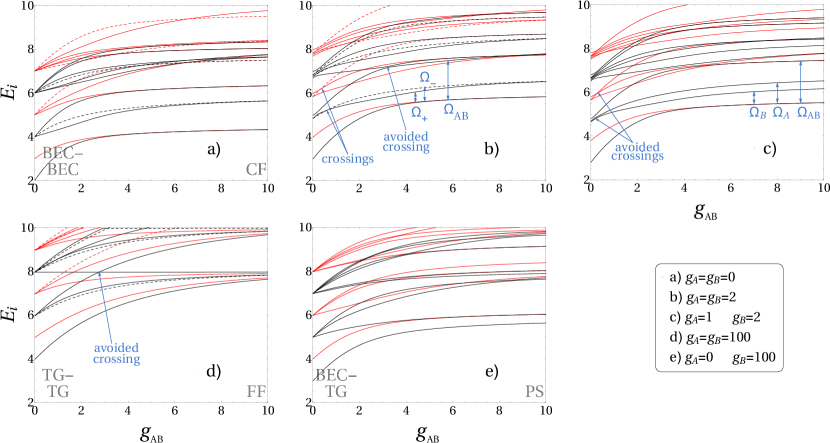
Figure 1: (Colour online) Energy spectrum of $H$ as a function of $g_{AB}$ for different fixed $g_{A}$ and $g_{B}$. The decoupled total CM is assumed to be in its ground state. The total parity is thus determined solely by the $R_{AB}$ parity and is marked by black lines (even states) and red lines (odd states). In Fig. a) b) d) solid curves correspond to symmetric ($+1$) and dashed to antisymmetric ($-1$) eigenstates under the $S_{r}$ operation. The indicated (avoided) crossings are exemplary and simply outline specific features. In b) and c), we label the excited states which are relevant for the lowest monopole excitations as discussed in Sect. V by the corresponding excitation frequencies $\Omega_{AB}$ etc. The labels for the ground-state phases in the limiting regimes BEC-BEC, TG-TG, etc. follow the nomenclature of García-March et al. (2014a), see also the main text. All quantities are given in HO units.

By means of the correlated basis introduced above and an efficient strategy for calculating the Hamiltonian matrix to be diagonalized (see Appendix A), we can easily obtain the static properties of our system for a huge variety of different intra- and inter-component interaction strengths. Before going into the details, we need to address the symmetries of $H$ in the relative frame.

Symmetry analysis

First of all, $H$ commutes with the individual parity operators $P_{Y_{i}}$ of the relative frame coordinates, $[H,P_{Y_{i}}]=0$. The eigenvectors of $P_{r_{\sigma}}$ are restricted to even parity because of the bosonic character of our components. Due to the decoupling of $H_{R_{CM}}$ it is sufficient to consider only the ground state of the total CM motion, which is of even $R_{CM}$ parity, in the following. Then, the parity of the $R_{AB}$ degree of freedom completely determines the total parity of the eigenstates. Another symmetry arises, if one chooses equal intra-component interaction strengths $g_{\sigma}$. Under these circumstances the Hamiltonian is invariant under $r_{A}\leftrightarrow r_{B}$ exchange, which we define as the $S_{r}$ transformation. It should be noted, that translating all these transformations to the laboratory frame leads to certain proper and improper rotations of the four-dimensional coordinate space.

Energy spectra

In Fig. 1 we show the total energy spectrum as a function of $g_{AB}$ for various fixed values of $g_{A}$ and $g_{B}$. The total CM is assumed to be in its ground state. Fig. 1(a) depicts the non-interacting intra-component scenario $g_{\sigma}=0$. For $g_{AB}=0$ the Hamiltonian represents two uncoupled non-interacting bosonic species and we will label this regime as BEC-BEC following the nomenclature of García-March et al. (2014a). The eigenenergies are integers with equal spacings of $\hbar w$, which is 1 in our units. In this limit the PCFs are even HO eigenstates of mass $m=1/2$. The eigenenergies are thus $E_{tot}=E_{n=0}^{CM}+E_{k,l,m}^{(0)}\equiv E_{0,k,l,m}^{(0)}=k+2l+2m+2$.

For $g_{AB}=0$, the $i$th eigenenergy corresponding to only even (odd) $R_{AB}$-parity eigenstates is $(i+2)!/(2!i!)$ fold degenerate with $i\in\mathbb{N}_{0}$. Already a small inter-component coupling lifts all these degeneracies such that branches of eigenenergies arise. In the following, we label these resulting branches as the $i$th even or odd $R_{AB}$-parity branch, respectively. Note that this grouping of the energy levels into branches will be used in the following for all values of $g_{AB}$ and in particular for the analysis of the breathing dynamics in section V. As we further increase the inter-component coupling strength, we observe that states corresponding to branches of opposite $R_{AB}$-parity incidentally cross, as they are of different symmetry and consequently not coupled by the $H_{1}$ perturbation.

For very strong $g_{AB}$ values, i.e. in the composite fermionization (CF) limit Zöllner et al. (2008); Hao and Chen (2009), we observe a restoration of degeneracies, but in a different manner, namely the lowest states merge pairwise forming a two-fold degeneracy. In this regime the two components spatially separate for the ground state, where one component locates on the left side of the trap, while the other is pushed to the right side due to the strong inter-component repulsion. The two-fold degeneracy of the ground state reflects actually the two possible configurations: A left B right and A right B left. This behaviour can be observed in the relative frame densities, discussed later in this section. Another striking peculiarity for $g_{AB}\rightarrow\infty$ are non-integer eigenvalues and unequal energy spacings.

A very similar analysis concerning this specific choice of interactions ($g_{\sigma}=0$ and arbitrary $g_{AB}$) was performed in Dehkharghani et al. (2015), where an effective interaction approach was employed to greatly improve the convergence properties of exact diagonalization in order to access properties of a Bose-Bose mixture up to $N=10$ particles. However, the analysis only covered a single line of the $(g_{A},g_{B},g_{AB})$ parameter space. Here, we extend the ground state analysis of García-March et al. (2014a) and study the low-lying excitations for arbitrary interactions.

In Fig. 1(b) we show the impact of moderate but symmetric intra-component interactions of strength $g\equiv g_{\sigma}=2$. Already in the uncoupled regime ($g_{AB}=0$) we observe fewer degeneracies compared to the $g_{\sigma}=0$ case. Nevertheless, we group the eigenstates into branches of even / odd $R_{AB}$-parity also for finite $g_{\sigma}$ by continuously following the eigenenergies to the $g_{\sigma}\rightarrow 0+$ limit. The reason for the reduced degeneracies is that PCFs are not HO eigenstates any more, while PCFs of both components are still the same. The energy is $E_{0,k,l,m}^{(0)}=k+\mu(g,l)+\mu(g,m)+2$. To roughly estimate the energetic ordering it is sufficient to know that the real-valued quantum number $\mu(g,n)$ fulfils for $0<g<\infty$ the following relations:

• $2n<\mu(g,n)<2n+1$

• $\mu(g,n)+1<\mu(g,n+1)<\mu(g,n)+2$

meaning that a single excitation of the relative motion $r_{\sigma}$ is energetically below a double excitation of the $R_{AB}$ degree of freedom. E.g. the first even $R_{AB}$-parity branch in the uncoupled non-interacting regime (BEC-BEC in Fig. 1(a)) contains three degenerate states: $|2,0,0\rangle$, $|0,1,0\rangle$ and $|0,0,1\rangle$ (eq. (9)). By choosing finite $g_{\sigma}$ values $|2,0,0\rangle$ acquires a higher energy than $|0,1,0\rangle$ and $|0,0,1\rangle$ leading to reduced degeneracies in the spectrum. Another striking feature is the appearance of additional crossings between states of the same $R_{AB}$-parity due to the $S_{r}$ symmetry. States, which possess different quantum numbers concerning the $S_{r}$ transformation ($+1$ or $-1$), are allowed to cross as they ’randomly’ do throughout the $g_{AB}$ variation. Of course, such crossings are also present in the previous non-interacting case, it being also component-symmetric. An avoided crossing between a state of the first even $R_{AB}$-parity branch and a state of the second even $R_{AB}$-parity branch is worth mentioning, which is present for all values of $g_{\sigma}$ (see the exemplary arrow in Fig. 1 (b) or (d)). States of the same symmetry obviously do not cross according to the Wigner-von Neumann non-crossing rule von Neumann and Wigner (1929).

In Fig. 1(c) we asymmetrically increase the intra-component interactions $g_{\sigma}$ as compared to the non-interacting case, namely to $g_{A}=1$ and $g_{B}=2$. For the uncoupled scenario ($g_{AB}=0$) all the degeneracies are lifted, because now PCFs of the $A$ and the $B$ components are different. The energy is $E_{0,k,l,m}^{(0)}=k+\mu(g_{A},l)+\mu(g_{B},m)+2$. The energetic state ordering is far from obvious, which becomes apparent upon closer inspection of the $\mu(g,n)$ function. E.g. consider again the first even $R_{AB}$-parity branch. Its lowest energy state is a single excitation of $r_{B}$, followed by a single excitation of $r_{A}$. The highest energy of this branch corresponds to a double $R_{AB}$ excitation. The ordering pattern for higher order branches is even more complicated. For intermediate values of $g_{AB}$ we observe that crossings from the previous scenario (with $g_{\sigma}=2$) between states of the same $R_{AB}$-parity are replaced by avoided crossings because of the broken $S_{r}$ symmetry. The strong coupling regime displays less degeneracies as compared to the component-symmetric cases of Fig. 1(a) and (b) with the two-fold ground state degeneracy remaining untouched.

In Fig. 1(d) we choose very strong intra-component interaction strengths $g_{\sigma}=100$. When the $g_{AB}$-coupling is absent, we have two hard-core bosons in each component. The system can thus be mapped to a two-component mixture of non-interacting fermions Girardeau (1960); Yukalov and Girardeau (2005) and will be referred to as TG-TG limit. The PCFs become near degenerate with odd HO eigenstates, which again leads to integer-valued eigenenergies $E_{0,k,l,m}^{(0)}\approx k+2l+2m+4$ with equal spacings and the same degree of (near-)degeneracies as in the non-interacting case (Fig. 1(a)). The limit of strong inter-component coupling displays a completely different structure of the spectrum. The so-called full fermionization (FF) Girardeau and Minguzzi (2007) phase can be mapped to a non-interacting ensemble of four fermions with the ground state energy $N^{2}/2=8$. However, in contrast to the single-component case of four bosons, we need to take into account that the components are distinguishable. The degeneracy of the ground state is expected to be $N!/(N_{A}!N_{B}!)=6$-fold and corresponds to the different possibilities of ordering the laboratory frame coordinates while keeping in mind the indistinguishability of particles of each component. A profound study of these ground states can be done by employing a snippet basis Deuretzbacher et al. (2008) of $N$ distinguishable particles, which interact with each other by an infinite repulsive delta-interaction. According to eq. (2) of Ref. Deuretzbacher et al. (2008), the snippet basis for distinguishable particles is defined as:

$$\langle x_{1},...,x_{N}|\Pi\rangle=\begin{cases}\sqrt{N!}|\Psi_{0}^{F}|&\quad\text{if}\quad x_{\Pi(1)}<...<x_{\Pi(N)}\\ 0&\quad\text{otherwise,}\end{cases}$$ (11)

where $\Psi_{0}^{F}$ represents the ground state of $N$ non-interacting fermions and $\Pi$ is a permutation of particle coordinates, which defines the sector where $\langle x_{1},...,x_{N}|\Pi\rangle$ has support. Every snippet state is one of $N!$ possible ground states in the hard-core limit.

To adjust this basis to our case one can follow a procedure described for a Bose-Fermi mixture in Fang et al. (2011). The only modification is to replace the antisymmetric exchange symmetry of the fermionic species by a symmetric one. With respect to the spatial projection $\langle\vec{x}|\equiv\langle x_{A,1},x_{A,2},x_{B,1},x_{B,2}|$ we will combine the $4!=24$ sectors of the distinguishable case into $6$ ground states of our Bose-Bose mixture. Each ground state consists of $4$ different sectors, reflecting the indistinguishability within each component, meaning that by exchanging the spatial order of identical particles we switch between these $4$ sectors. By exchanging the spatial order of distinguishable particles we switch between the different ground states. Thus, the permutations $\Pi=\tau\ \kappa$ can be decomposed in transpositions $\tau$ which exchange identical particles and transpositions $\kappa$ which exchange distinguishable particles, leading to the following ground state configurations:

$$\Psi_{AABB} \propto\langle\vec{x}|(e+(1,2))(e+(3,4))\ (e)\rangle,$$

$$\Psi_{BBAA} \propto\langle\vec{x}|(e+(3,4))(e+(1,2))\ (1,3)(2,4)\rangle,$$

$$\Psi_{ABAB} \propto\langle\vec{x}|(e+(1,3))(e+(2,4))\ (2,3)\rangle,$$

$$\Psi_{BABA} \propto\langle\vec{x}|(e+(2,4))(e+(1,3))\ (1,4)\rangle,$$

$$\Psi_{ABBA} \propto\langle\vec{x}|(e+(1,4))(e+(2,3))\ (2,4)\rangle,$$

$$\Psi_{BAAB} \propto\langle\vec{x}|(e+(2,3))(e+(1,4))\ (1,3)\rangle,$$

where the $(i,j)$ notation describes the exchange of particles $i\leftrightarrow j$, $e$ is the identity permutation and for two permutations $\Pi_{1}$, $\Pi_{2}$, $\langle\vec{x}|\Pi_{1}+\Pi_{2}\rangle$ is defined as $\langle\vec{x}|\Pi_{1}\rangle+\langle\vec{x}|\Pi_{2}\rangle$. The sub-index of the wave-function $\Psi$ relates to the particle arrangements in the one-body density distribution.

The last case we discuss is the highly asymmetric case $g_{A}=0$ and $g_{B}=100$ in Fig. 1(e). For $g_{AB}=0$ (BEC-TG) one expects, based on the previous considerations, integer eigenvalues $E_{0,k,l,m}^{(0)}\approx k+2l+2m+3$ and thus equal spacings as for the cases $g_{\sigma}=0$ and $g_{\sigma}=100$ depicted in Fig. 1(a) and (d), because the PCF of the $A$ component is an even HO eigenstate and the PCF of the $B$ component is degenerate with an odd HO eigenstate. Very peculiar is the strong coupling case, where we observe a non-degenerate ground state, the so-called phase separation (PS) phase García-March et al. (2014a), where the $A$ component occupies the centre of the harmonic trap, while the $B$ component, in order to reduce its intra-component interaction energy, forms a shell around the $A$ component.

Relative-frame densities

Figure 2: Ground state relative frame probability densities: a) $\rho_{1}^{(0)}(R_{AB})$ b) $\rho_{1}^{(0)}(r_{A})$ and c) $\rho_{1}^{(0)}(r_{B})$. The depicted limiting cases are BEC-BEC ($g_{\sigma}=g_{AB}=0$), TG-TG ($g_{\sigma}=100$, $g_{AB}=0$), CF ($g_{\sigma}=0$, $g_{AB}=10$) and PS ($g_{A}=0$, $g_{B}=100$, $g_{AB}=10$). All quantities are given in HO units.

Let us now inspect the relative-frame probability densities $\rho_{1}(Y_{i})$ instead of the usually studied one-body densities $\rho_{1}(x_{\sigma})$ of the laboratory frame as e.g. in García-March et al. (2014a). We will see that these quantities can be used to identify regions of most probable relative distances and provide a more detailed picture of particle arrangements than their laboratory frame counterparts. Moreover, in the quench dynamics study, the subject of the next section, an occupation of a certain eigenstate of $H$ will lead to the breathing oscillation of only one relative-frame density, making it possible to connect different breathing modes to specific relative motions within the system, at least for the weakly coupled case $g_{AB}\ll 1$.

We define these quantities as follows:

$$\rho_{1}^{(j)}(Y_{i})=\int\prod_{p\neq i}dY_{p}\ |\langle\vec{Y}|E_{j}\rangle|^{2},$$ (12)

where $|E_{j}\rangle$ is the $j$-th eigenstate of $H$ and we trace out all the degrees of freedom of the relative frame $\vec{Y}$ except for one.

Let’s compare our results concerning the ground state densities for some limiting cases to the ones obtained in García-March et al. (2014a). In Fig. 2 we show the densities for all the degrees of freedom except for $R_{CM}$, which trivially obeys a Gaussian distribution. In the BEC-BEC case all the densities are characterized by a Gaussian density profile, since the Hamiltonian consists of completely decoupled HOs for each degree of freedom. The TG-TG limit differs from the BEC-BEC case in the $\rho_{1}^{(0)}({r_{\sigma}})$ distributions featuring two maxima and a minimum in between, a result of strong repulsion within each component. This behaviour reflects actually the already known results of the analytical two-particle solution Busch et al. (1998), where $\rho_{1}^{(0)}(r)$ develops a minimum in the centre of the density distribution for finite $g$ whose value tends to zero as $g\rightarrow\infty$.

The CF phase is in some sense a complete counter-part to the TG-TG case. Now $\rho_{1}^{(0)}(R_{AB})$ features two maxima and a minimum in between, a result of A and B strongly repelling each other. This feature is blurred in the one-body density distributions $\rho_{1}^{(0)}(x_{\sigma})$ of the laboratory frame and one needs to additionally consider the two-body density function $\rho_{2}^{(0)}(x_{A},x_{B})$ to verify this behaviour Zöllner et al. (2008). The density distribution of $\rho_{1}^{(0)}(r_{\sigma})$ is more compressed compared to the BEC-BEC case due to the tighter confinement induced by the other component.

Finally, the PS phase corresponds to a core-shell structure, where $\rho_{1}^{(0)}(R_{AB})$ and $\rho_{1}^{(0)}(r_{A})$ show a more pronounced peak, while $\rho_{1}^{(0)}(r_{B})$ obeys a bimodal distribution with two density peaks being much further apart than both in the CF and in the TG-TG case. This can be understood in the following way: firstly, the fact that A locates in the trap centre and not the other way around is because B needs to minimize its repulsive intra-component interaction energy by separating its particles. Secondly, the need to minimize the repulsive inter-component energy pushes the B particles even further along the harmonic trap at the cost of increased potential energy until these two energies balance themselves out. The two A particles are compressed to closer distances as compared to the BEC-BEC case because of a tighter trap induced by B, while at the same time A modifies the HO potential to a double well for B. This results in stronger localization of particles, which leads to a more pronounced peak in the $R_{AB}$ distribution.

V Breathing Dynamics

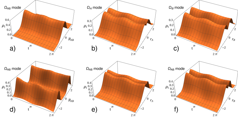
Figure 3: (Colour online) Relative frame density modulations for the component-asymmetric case of Fig. 1 (c). Subfigs. (a)-(c): The decoupled regime $g_{AB}=0$. (a) $\rho_{1}(R_{AB},t)$ oscillates solely due to $|2,0,0\rangle$ eigenstate with the frequency $\Omega_{AB}=2$, (b) $\rho_{1}(r_{A},t)$ due to $|0,1,0\rangle$ with the frequency $\Omega_{A}$, (c) $\rho_{1}(r_{B},t)$ due to $|0,0,1\rangle$ with the frequency $\Omega_{B}$. Subfigs. (d)-(f): Strongly coupled regime $g_{AB}=10$. (d) $\rho_{1}(R_{AB},t)$, (e) $\rho_{1}(r_{A},t)$, (f) $\rho_{1}(r_{B},t)$. All the profiles oscillate with the same frequency $\Omega_{AB}$. Not shown is the breathing motion of $\rho_{1}(R_{CM},t)$ with the constant frequency of $\Omega_{CM}=2$, it being a decoupled motion of a single-particle HO. Quench strength $\delta\omega=-0.1$. All quantities are given in post-quench HO units.

The spectral properties discussed above can be probed by slightly quenching a system parameter such that the lowest lying collective modes are excited. Here, we focus on a slight quench of the trapping frequency in order to excite the breathing or monopole modes being characterized by a periodic expansion and compression of the atomic density. While in the single-component case two lowest lying breathing modes of in general distinct frequencies exist, being associated with a motion of the CM and the relative coordinates Bauch et al. (2009); Schmitz et al. (2013), respectively, the number of breathing modes, their frequencies and the associated “normal coordinates” are so far unknown for the more complex case of a binary few-body mixture and shall be the subject of this section.

Experimentally, breathing oscillations can be studied by measuring the width of $\sigma$ species density distribution $\int dx_{\sigma}\ x_{\sigma}^{2}\rho_{1}(x_{\sigma},t)$ where we have omitted the subtraction of the mean value $\int dx_{\sigma}\ x_{\sigma}\rho_{1}(x_{\sigma},t)$ squared, which vanishes due to the parity symmetry. From a theoretical point of view, it is fruitful to define a breathing observable as $\sum_{\sigma,i}x_{\sigma,i}^{2}$, whose expectation value is essentially the sum of the widths of the A and the B component.

To study the breathing dynamics we will perform a slight and component-symmetric quench of the HO trapping frequency, where our HO units will be given with respect to the post-quench system. The initial state for the time-propagation is the ground state $|\Psi(t=0)\rangle=|E_{0}\rangle_{\omega_{0}}$ of some pre-quench Hamiltonian with frequency $\omega_{0}\gtrsim 1$. Then a sudden quench is performed to $\omega=1$. The time evolution of this state is thus described as follows:

$$|\Psi(t)\rangle=e^{-iHt}|E_{0}\rangle_{\omega_{0}}\approx\sum_{j=0}^{n}c_{j}e^{-iE_{j}t}|E_{j}\rangle,$$ (13)

where $|E_{j}\rangle\equiv|E_{j}\rangle_{\omega}$ and $c_{j}=\langle E_{j}|E_{0}\rangle_{\omega_{0}}$ is the overlap between the initial state and the $j$th eigenstate $|E_{j}\rangle$ of the post-quench Hamiltonian $H$. Since both the pre- and post-quench Hamiltonian are time-reversal symmetric, we assume their eigenstates and thereby also the overlap coefficients $c_{j}$ to be real-valued without loss of generality. A small quench ensures that $|c_{0}|\approx 1$ and only the $n$ lowest excited states are of relevance. Symmetry considerations further reduce the number of allowed contributions. E.g. states of odd $R_{CM}$-parity or odd $R_{AB}$-parity have zero overlap with $|E_{0}\rangle_{\omega_{0}}$, because the initial state is of even $R_{CM}$- and $R_{AB}$-parity and the quench does not affect any of the symmetries discussed in the previous section. Similarly, in the component-symmetric case $g_{A}=g_{B}$, states, which are antisymmetric w.r.t. the $S_{r}$ operation, have no overlap with the pre-quench ground state being symmetric under $S_{r}$.

For the weakly coupled regime, the relative-frame coordinates turn out to be extremely helpful for characterizing the participating breathing modes. Therefore, we study in particular the reduced densities of the relative-frame coordinates. Employing the expansion in post-quench eigenstates from eq. (13), their time-evolution may be approximated within the linear-response regime as

$$\rho_{1}(Y_{i},t)\approx c_{0}^{2}\rho_{1}^{(0)}(Y_{i})+2\sum_{j=1}^{n}c_{0}c_{j}\rho_{1}^{(0,j)}(Y_{i})\cos(\Delta_{j}t),$$ (14)

neglecting terms of the order $c_{i}c_{j}$ for $i,j>0$. So $\rho_{1}(Y_{i},t)$ can be decomposed into the stationary background $\rho_{1}^{(0)}(Y_{i})$ and time-dependent modulations of the form $\rho_{1}^{(0,j)}(Y_{i})=\int\prod_{p\neq i}dY_{p}\ \langle\vec{Y}|E_{0}\rangle\langle E_{j}|\vec{Y}\rangle$, further called transition densities, with oscillation frequency $\Delta_{j}=E_{j}-E_{0}$.

In the following, we regard the excitations of the first even $R_{AB}$-parity branch as the lowest monopole modes and show that each monopole mode is directly connected to the breathing modulation of a single relative-frame density, if the two components are but weakly coupled. This behaviour changes for increasing $g_{AB}$, where each coordinate begins to exhibit an oscillation with more than one frequency. By inspecting the modulations of the variances of each relative-coordinate and taking the excitation amplitudes into account, we show that four (three) breathing modes are excited for $g_{A}\neq g_{B}$ ($g_{A}=g_{B}$) in the weakly coupled regime, while only two breathing modes are of relevance in the strongly coupled regime. First, we inspect the component-asymmetric case of Fig. 1(c) in detail to illustrate some peculiarities of involved breathing modes, since it contains the most relevant features. Thereafter, we unravel differences to the component-symmetric case of Fig. 1(b).

V.1 Component-asymmetric case

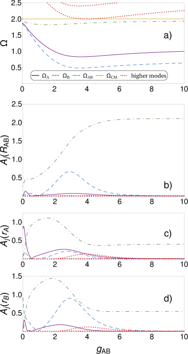
Figure 4: (Colour online) (a) Breathing mode frequencies as a function of the inter-component coupling $g_{AB}$ for the component-asymmetric case $g_{A}=1.0$ and $g_{B}=2.0$. The modes are labelled with respect to the uncoupled regime, where each mode can be identified with a particular relative-frame motion (Fig. 3 (a)-(c)). (b)-(d) Amplitudes $A_{j}$ (eq. (20)) of the modes depicted in (a) (same color coding), which determine the relevance of the contribution to the oscillation of the observable $Y_{i}^{2}$ as a function of the inter-component coupling $g_{AB}$: (b) $A_{j}(R_{AB})$, (c) $A_{j}(r_{A})$, (d) $A_{j}(r_{B})$. The red dotted lines stem from the states of the second even $R_{AB}$-parity branch. All quantities are given in post-quench HO units.

Because of the low amplitude quenching protocol, we will excite four breathing modes simultaneously in the component-asymmetric case ($g_{A}=1$, $g_{B}=2$). Three of them stem from the first even $R_{AB}$-parity branch of Fig. 1(c). Remember, however, that the total CM was assumed to be in the ground state to keep the spectrum discernible. One obtains the full spectral picture by including all CM excitations, meaning duplicating and up-shifting depicted energy curves by $\Delta E=n$ with $n\in\mathbb{N}$. This reveals a forth mode, namely a double total CM excitation. It features the same parity symmetries and is energetically of the same order as the states from the first even $R_{AB}$-parity branch ensuring a considerable overlap with the initial state. The total CM trivially oscillates with the constant frequency $\Omega_{CM}=2$ independent of any interactions $g_{\alpha}$ it being a decoupled degree of freedom with the single-particle HO Hamiltonian (eq. (5)) Bauch et al. (2010); Schmitz et al. (2013). The other three modes, which are excited, are known analytically, when there is no coupling between the components, and we label the corresponding mode frequencies as:

1. $|0\rangle|0,1,0\rangle\ \leftrightarrow\ \Omega_{A}(g_{AB}=0)=\mu(g_{A},1)-\mu(g_{A},0)$,

2. $|0\rangle|0,0,1\rangle\ \leftrightarrow\ \Omega_{B}(g_{AB}=0)=\mu(g_{B},1)-\mu(g_{B},0)$,

3. $|0\rangle|2,0,0\rangle\ \leftrightarrow\ \Omega_{AB}(g_{AB}=0)=2$,

4. $|2\rangle|0,0,0\rangle\ \leftrightarrow\ \Omega_{CM}=2$,

where we have prepended the CM eigenstate $|n\rangle$ for a complete characterization of the involved states. States of higher order even $R_{AB}$-parity branches as well as higher excitations of the CM coordinate are negligible due to small overlaps with the initial state.

In the uncoupled regime $g_{AB}=0$, one can show analytically that each relative-coordinate density oscillates with a single frequency, each corresponding to exactly one eigenstate of the first even $R_{AB}$-parity branch (see Fig. 3 (a)-(c)). E.g. for $\rho_{1}(R_{AB},t)$, the only transition density $\rho_{1}^{(0,j)}(R_{AB})$ which survives taking the partial trace is the one corresponding to $|0\rangle|2,0,0\rangle$, while the contributions from the remaining excited states vanish. This leads to the breathing motion in the $R_{AB}$ coordinate with a single frequency $\Omega_{AB}$. Analogously one can show that $|0\rangle|0,1,0\rangle$ solely induces density modulation in $\rho_{1}(r_{A})$ with the frequency $\Omega_{A}$, while $\rho_{1}(r_{B})$ oscillates with $\Omega_{B}$ exclusively due to $|0\rangle|0,0,1\rangle$. Thereby, the relative-frame coordinates render “normal coordinates” in the uncoupled regime, which is also a valid picture for extremely weak couplings.

By introducing a larger coupling between the components one observes that each relative frame density, except for $\rho_{1}(R_{CM},t)$, begins to oscillate with up to three frequencies simultaneously. So all the modes begin to contribute to the density modulation of each relative coordinate. However, there are some peculiarities we observe, for the visualization of which the densities are not well suited any more. Instead, we will transform the breathing observable to the relative frame and consider the expectation values of individual terms it decomposes into:

$$\sum_{\sigma,i}x_{\sigma,i}^{2}=4R_{CM}^{2}+R_{AB}^{2}+\frac{1}{2}r_{A}^{2}+\frac{1}{2}r_{B}^{2}.$$ (15)

The expectation value of each observable with respect to the time-evolved state $|\Psi(t)\rangle$ is directly related to the respective relative-frame density:

$$\langle\Psi(t)|Y_{i}^{2}|\Psi(t)\rangle=\int dY_{i}\ Y_{i}^{2}\ \rho_{1}(Y_{i},t).$$ (16)

Inserting the time-evolution of the relative frame density from eq. (14) one finds that the observables decompose into a stationary value and a time-dependent modulation as well. In particular, we are interested in the amplitudes of modulations, when the inter-component coupling is varied, since they determine how many frequencies are of essential relevance for the considered motion. The amplitude of the $j$th mode is essentially composed of the overlap $c_{j}$ and of the transition element:

$$\langle E_{j}|Y_{i}^{2}|E_{0}\rangle=\int dY_{i}\ Y_{i}^{2}\ \rho_{1}^{(0,j)}(Y_{i}).$$ (17)

In order to evaluate the overlaps $c_{j}=\langle E_{j}|E_{0}\rangle_{\omega_{0}}$ with $j\neq 0$ in terms of only the post-quench Hamiltonian eigenstates, we perform a Taylor approximation with respect to the weak quench strength $\delta\omega=\omega-\omega_{0}$, namely $|E_{0}\rangle_{\omega_{0}}\approx|E_{0}\rangle_{\omega}-\delta\omega\frac{d}{d\omega}|E_{0}\rangle_{\omega}$ evaluated at $\omega=1$, and arrive at

$$c_{j}\approx-\langle E_{j}|\frac{d}{d\omega}|E_{0}\rangle\delta\omega.$$ (18)

Applying the (off-diagonal) Hellmann-Feynman theorem, one obtains:

$$\langle E_{j}|\frac{d}{d\omega}|E_{0}\rangle=\frac{-\omega\langle E_{j}|\sum_{i,\sigma}x_{i,\sigma}^{2}|E_{0}\rangle}{E_{j}-E_{0}}.$$ (19)

The overlaps are hence connected to the transition elements of each relative-frame breathing observable (eq. (15)), weighted with the inverse of the mode frequency, which leads to a damping of contributions from higher order branches. This relation enables us to calculate the amplitude $A_{j}$, with which the $j$-th mode contributes to the oscillation of the observable $Y_{i}^{2}$:

$$A_{j}(Y_{i})=\left|\frac{c_{j}}{\delta\omega}\langle E_{j}|Y_{i}^{2}|E_{0}\rangle\right|,$$ (20)

which may be interpreted as the susceptibility of the $Y_{i}^{2}$ observable for the excitation of the state $|E_{j}\rangle$.

In Fig. 4 (a) we show the values of possible breathing mode frequencies, obtained from the spectrum of Fig. 1 (c). $\Omega_{CM}=2$ does not depend on any interactions $g_{\alpha}$. In contrast to this, $\Omega_{AB}$ is degenerate with $\Omega_{CM}$ for $g_{AB}=0$, and when increasing $g_{AB}$, decreases to a minimum first and then increases with the tendency to asymptotically reach $\Omega_{CM}$ again. This behaviour strongly resembles the dependence of the relative-coordinate breathing-mode frequency in the single-component case Schmitz et al. (2013). $\Omega_{A}$ and $\Omega_{B}$ have qualitatively akin curve shapes, varying much stronger with $g_{AB}$. In particular, we note that these frequencies reach values below the frequency of the CM dipole mode being equal to unity.

The breathing mode frequencies discussed above are labelled according to the peculiarity of the uncoupled regime, where each eigenstate from the first even $R_{AB}$-parity branch leads to a breathing motion of some specific relative-frame coordinate. Indeed, if we look at the amplitudes $A_{j}$ in Fig. 4 (b)-(d) in the decoupled regime ($g_{AB}=0$), we recognize that the amplitude for the coordinate $Y_{i}$ is non-zero only for one mode, namely the one with which $\rho_{1}(Y_{i},t)$ oscillates in Fig. 3 (a)-(c). When we increase the inter-component coupling, the eigenstates cease to be simple product states in the relative coordinate frame resulting in contamination of each density modulation with the frequencies from the other modes as well, which leads to a three-mode oscillation. Nevertheless, we label the frequencies corresponding to the uncoupled case and follow the states continuously throughout the $g_{AB}$ variation.

Another peculiarity worth noting arises in the strongly coupled regime: $\Omega_{\sigma}$ oscillations become strongly suppressed for all the observables making $\Omega_{AB}$ and $\Omega_{CM}$ the main contributors to the density modulations. In Fig. 3 (d)-(f) we show that all the relative-coordinate densities oscillate with the same frequency $\Omega_{AB}$. We highlight that in the CF regime each density peak of the bimodal distribution $\rho_{1}(R_{AB},t)$ does not only breath periodically but also its maximum height position performs dipole-mode like oscillations, see Fig. 3 (d).

V.2 Component-symmetric case

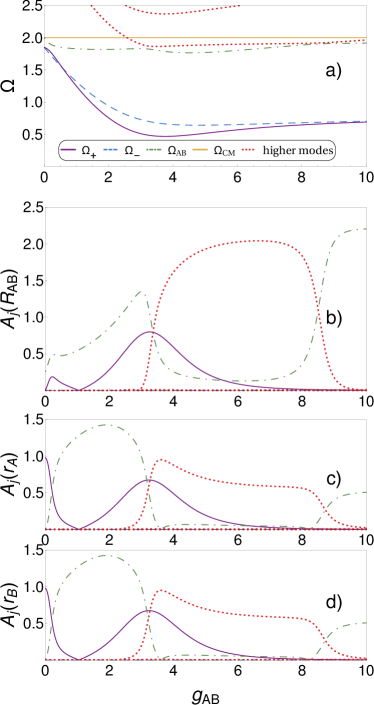
Figure 5: (Colour online) (a) Breathing mode frequencies as a function of the inter-component coupling $g_{AB}$ for the component-symmetric case $g_{\sigma}=2.0$. (b)-(d) Amplitudes $A_{j}$ (eq. (20)) of the modes shown in (a) (same color pattern), which determine the relevance of the contribution to the oscillation of the observable $Y_{i}^{2}$ as a function of the inter-component coupling $g_{AB}$: (b) $A_{j}(R_{AB})$, (c) $A_{j}(r_{A})$, (d) $A_{j}(r_{B})$. The red dotted lines stem from the states of the second even $R_{AB}$-parity branch. All quantities are given in post-quench HO units.

Now we compare the above results with the component-symmetric case of Fig. 1 (b), where $g_{A}=g_{B}=2$. Fig. 5 (a) depicts the possible breathing-mode frequencies. Here, two main differences arise: First, the $\Omega_{AB}$ curve features two minima due to two avoided crossings with an eigenstate of the second even $R_{AB}$-parity branch. Second, the other two breathing mode frequencies of the relative coordinates are degenerate for $g_{AB}=0$, then separate with increasing $g_{AB}$ and approach one another asymptotically. Instead of using the labels $\Omega_{A}$ and $\Omega_{B}$ as in the component-asymmetric case, we label these two modes with $\Omega_{+}$ and $\Omega_{-}$, since the corresponding excited eigenstates are symmetric and antisymmetric w.r.t. $S_{r}$, respectively (see Fig. 1 (b)). The latter frequency, however, does not give any contribution to the breathing dynamics, it being symmetry excluded.

The motion of the $r_{A}$ and $r_{B}$ coordinates is identical due to the imposed component-symmetry and in the uncoupled regime ($g_{AB}=0$) they both oscillate solely with the $\Omega_{+}$ frequency (see Fig. 5 (c) and (d)). Similarly to the component-asymmetric case, we see that when increasing $g_{AB}$ the $\Omega_{AB}$ ($\Omega_{+}$) mode contributes also to the observable $r_{\sigma}^{2}$ ($R_{AB}^{2}$).

However, in the intermediate interaction regime ${3.7\lesssim g_{AB}\lesssim 8.3}$ we observe a strong suppression of the $\Omega_{AB}$ mode contribution for all observables, which is in stark contrast to the component-asymmetric case. Instead, a state of the second even $R_{AB}$-parity branch gains relevance. These two eigenstates actually participate in the avoided crossing exemplary indicated by an arrow in the spectrum (see Fig. 1 (b)) and thereby exchange their character. By further increasing $g_{AB}$ we observe another exchange of roles, which is attributed to the presence of a second avoided crossing (see Fig. 5 (a)), such that the strong inter-component coupling regime shows again the absolute dominance of the $\Omega_{AB}$ mode over the other lowest breathing modes besides $\Omega_{CM}$.

VI Experimental realization

The few-body Bose-Bose mixture studied here should be observable with existing cold atom techniques. Quantum gas microscopes allow the detection of single particles in a well controlled many-body or few-body system Bakr et al. (2010); Sherson et al. (2010) and recent progress also allows for spin-resolved imaging in 1D systems using an expansion in the perpendicular direction Preiss et al. (2015); Boll et al. (2016). In these set-ups, the single-particle sensitivity relies on pinning the atoms in a deep lattice during imaging and experiments have so far focused on lattice systems. However, bulk systems might be imaged with high spatial resolution by freezing the atomic positions in a lattice before imaging. For fast freezing, this would allow a time-resolved measurement of the breathing dynamics. Moreover, spin order was recently observed in very small fermionic bulk systems via spin-selective spilling to one side of the system Murmann et al. (2015).

Deterministic preparation of very small samples was demonstrated for fermions via trap spilling Serwane et al. (2011) and for bosons by cutting out a subsystem of a Mott insulator Islam et al. (2015). The tight transverse confinement for a 1D system can be obtained from a 2D optical lattice, while the axial confinement would come from an additional optical potential, which can be separately controlled to initialize the breathing mode dynamics.

Choosing two hyperfine states of the same atomic species ensures the same mass of the two bosonic species. Possible choices include ${}^{7}Li$, ${}^{39}K$ or ${}^{87}Rb$. While the former have usable FRs to tune the interaction strengths, the latter allows selective tuning via CIR in a spin-dependent transversal confinement as can be realized for heavier elements. Note that the longitudinal confinement needs to be spin-independent in order to ensure the same longitudinal trap frequencies and trap centres assumed in the calculations. The inter-component interaction strength can be tuned via a transverse spatial separation as obtained e.g. from a magnetic field gradient Schachenmayer et al. (2015). In the case of ${}^{7}Li$ and ${}^{39}K$, the inter-component background scattering lengths are negative Chin et al. (2010) leading to negative $g_{AB}$, but although not reported, inter-component FRs might exist. Alternatively, $g_{AB}$ might be tuned via a CIR, which selectively changes $g_{AB}$ at magnetic fields, where the intra-component scattering lengths are very different.

In the following we give concrete numbers for a choice of ${}^{7}Li$. The density distribution has structures on the scale of the HO unit $a_{ho}$ (Fig. 2). Choosing the trap parameters as in Ref. Serwane et al. (2011) as $\omega/(2\pi)=1.5$ kHz and $\omega_{\perp}/(2\pi)=15$ kHz, yields $a_{ho}=1$ $\mathrm{\mu m}$, i.e. larger than a typical optical resolution of $0.8$ $\mathrm{\mu m}$. At the same time, temperatures much lower than $\hbar\omega/k_{B}=72$ nK are state of the art. The breathing dynamics will occur on a time scale of several $100$ $\mathrm{\mu s}$, which is easily experimentally accessible. Choosing a smaller $\omega$ would make the imaging easier, but would impose stricter requirements on the temperature.

For the observation of the breathing mode dynamics, one would record the positions of all four particles in each experimental image and obtain the widths $\langle R_{CM}^{2}\rangle_{t}$, $\langle R_{AB}^{2}\rangle_{t}$, $\langle r_{\sigma}^{2}\rangle_{t}$ by averaging the occurring relative coordinates over many single-shots after a fixed hold time $t$.

VII Discussion and Outlook

In this work we have explored a few-body problem of a Bose-Bose mixture with two atoms in each component confined in a quasi-1D HO trapping potential by exact diagonalization. By applying a coordinate transformation to a suitable frame we have constructed a rapidly converging basis consisting of HO and PCF eigenfunctions. The latter stem from the analytical solution of the relative part of the two-atom problem Busch et al. (1998) and include the information about the intra-species correlations, which renders our basis superior to the common approach of using HO eigenstates as basis states.

We have then explored the behaviour of the low-lying energy spectrum as a function of the inter-species coupling for various fixed values of intra-species interaction strengths. Hereby we have covered the strongly coupled limiting cases of Composite Fermionization, Full Fermionization and Phase Separation, studied also intermediate symmetric and asymmetric values of $g_{A}$ and $g_{B}$ and related the ground state relative-frame densities of some limiting cases to the known laboratory frame results García-March et al. (2014a). We have discussed the evolution of degeneracies and explained appearing (avoided) crossings in terms of the symmetries of the Hamiltonian, which become directly manifest in the chosen relative-coordinate frame.

Finally, the obtained results were used to study the dynamics of the system under a slight component-symmetric quench of the trapping potential. We have derived expressions for the time evolution of the relative-frame densities within the linear response regime and observed that in the uncoupled regime ($g_{AB}=0$) the density of each relative frame coordinate performs breathing oscillations with a single frequency corresponding to a specific excited state of the first even $R_{AB}$-parity branch of the spectrum. The total CM coordinate performs breathing oscillations with the frequency $\Omega_{CM}=2$ (HO units). For asymmetric choices of $g_{\sigma}$ values, three additional monopole modes participate in the dynamics, each of them corresponding to the motion of a particular relative coordinate: $\Omega_{A}$ for the relative coordinate of the A component, $\Omega_{B}$ for the relative coordinate of the B component and $\Omega_{AB}$ for the relative distance of the CMs of both components. In contrast to this, the symmetric case $g_{A}=g_{B}$ leads to only two additional modes because of a symmetry-induced selection rule: $\Omega_{+}$ for the relative coordinates of both components and $\Omega_{AB}$ for the relative distance of the CMs of both components.

For not too strong inter-component coupling, each relative coordinate exhibits multi-mode oscillations and we have explored their relevance for the density modulations by analysing the behaviour of suitably chosen observables as one gradually increases the coupling between the components for symmetric and asymmetric choices of intra-component interactions strengths. Thereby, we have found that for strong couplings, where Composite Fermionization takes place, the $\Omega_{\sigma}$ ($\Omega_{+}$) modes become highly suppressed, leaving only two monopole modes in this regime: $\Omega_{AB}$ and $\Omega_{CM}$. We have observed the same effect for the case of Phase Separation (results not shown). Interestingly, the dependence of $\Omega_{AB}$ on $g_{AB}$ strongly resembles the behaviour of the relative-coordinate breathing frequency in the single-component case Schmitz et al. (2013). All in all, we have obtained 2 to 4 monopole modes for the quench dynamics depending on the strength of the inter-component coupling and the symmetry of the intra-species interactions, which is in strong contrast to the single-component case Schmitz et al. (2013) as well as to the MF results, where two low-lying breathing modes can be obtained, namely an in-phase (out-of-phase) mode for a component-symmetric (component-asymmetric) quench Morise and Wadati (2000). Finally, we have argued that the experimental preparation of the considered few-body mixture and measurement of the predicted effects are in reach by means of state-of-the-art techniques.

This work serves as a useful analysis tool for future few-body experiments. Measurements of the monopole modes can be mapped to the effective interactions within the system such that precise measurements of the scattering lengths or external magnetic fields can be performed. The numerical method used here can be applied to Bose-Fermi and Fermi-Fermi mixtures with two particles in each component simplifying the numerics, because the PCFs have to be replaced by odd HO eigenstates, if a bosonic component is switched to a fermionic one, which significantly accelerates the calculation of integrals. Further, it would be interesting to see how the frequencies and the amplitudes of the monopole modes vary for an increasing number of particles. Exploring the spectrum for negative values of interaction parameters is also a promising direction of future research.

Appendix A

In the following, we discuss how to efficiently calculate matrix elements of the coupling operator $H_{1}$ from eq. (8) with respect to the basis (9). Because of the already mentioned even parity of $\varphi^{\sigma}_{i}$ one can make simple substitutions of the form $\tilde{r}_{\sigma}=-r_{\sigma}$ to show that each delta in the sum of $H_{1}$ gives the same contribution, such that after performing an integral over $R_{AB}$ one obtains:

$$\langle a,b,c|H_{1}|k,l,m\rangle=$$

$$4\int dr_{A}\int dr_{B}\ \Phi_{a}^{AB}\left(\frac{r_{A}+r_{B}}{2}\right)\Phi_{k}^{AB}\left(\frac{r_{A}+r_{B}}{2}\right)$$

$$\varphi_{b}^{A}(r_{A})\varphi_{l}^{A}(r_{A})\varphi_{c}^{B}(r_{B})\varphi_{m}^{B}(r_{B}).$$ (21)

At this point it is important to notice that the integral vanishes for odd $(a+k)$ because of the parity symmetries of $\Phi^{AB}$ and $\varphi^{\sigma}$, which can be seen by transforming to relative and center-of-mass coordinates $r=r_{A}-r_{B}$, $R=(r_{A}+r_{B})/2$. In the following, we assume that the quantum numbers for the $R_{AB}$ coordinate are restricted to $a,k\in\{1,...,n_{AB}\}$ and for the $r_{\sigma}$ coordinates to $b,c,l,m\in\{1,...,n_{\rm rel}\}$. Now our computation strategy consists of three steps:

First, we circumvent evaluating the 2D integral from eq. (21) by viewing the product of the two HO eigenstates $\Phi_{a}^{AB}\Phi_{k}^{AB}$ as a pure, in general not normalized state $\chi_{a,k}$ depending on the two coordinates $r_{A}$ and $r_{B}$ and applying the Schmidt decomposition Nielsen and Chuang (2000) or, equivalently, the so-called POTFIT algorithm Jäckle and Meyer (1996).

$$\chi_{a,k}(r_{A},r_{B}) \equiv\Phi_{a}^{AB}\left(\frac{r_{A}+r_{B}}{2}\right)\Phi_{k}^{AB}\left(\frac{r_{A}+r_{B}}{2}\right)$$

$$\approx\sum_{i=0}^{d}\lambda_{i}^{(a,k)}w_{i}^{A;(a,k)}(r_{A})w_{i}^{B;(a,k)}(r_{B}).$$

Here, $|\lambda^{(a,k)}_{i}|^{2}$ coincides with the $i$th eigenvalue of the reduced one-body density matrix corresponding to the degree-of-freedom $r_{\sigma}$ and $w_{i}^{\sigma;(a,k)}(r_{\sigma})$ denotes the corresponding eigenvector, which can be shown to feature a definite parity symmetry. We remark that (i) we may choose $w_{i}^{A;(a,k)}(r)=w_{i}^{B;(a,k)}(r)\equiv w_{i}^{(a,k)}(r)$ because of $\chi_{a,k}(r_{A},r_{B})=\chi_{a,k}(r_{B},r_{A})$ without loss of generality and that (ii) the decomposition of eq. (A) becomes exact for $d\rightarrow\infty$. Having ordered the coefficients $\lambda^{(a,k)}_{i}$ in decreasing sequence w.r.t. to their modulus, we choose $d$ such that only terms with $|\lambda^{(a,k)}_{i}/\lambda^{(a,k)}_{0}|>10^{-6}$ are taken into account, which results in an accurate approximation to $\chi_{a,k}$. We perform this decomposition for all the relevant HO quantum numbers $(a,k)$, meaning $a\leq k\leq n_{AB}$ with $(a+k)$ even. This procedure is independent of any interactions $g_{\alpha}$ and needs to be executed only once.

By inserting eq. (A) into eq. (21) we obtain the following expression:

$$\langle a,b,c|H_{1}|k,l,m\rangle\approx$$

$$4\sum_{i=0}^{d}\lambda_{i}^{(a,k)}\int dr_{A}\ w_{i}^{(a,k)}(r_{A})\varphi_{b}^{A}(r_{A})\varphi_{l}^{A}(r_{A})$$

$$\qquad\qquad\quad\int dr_{B}\ w_{i}^{(a,k)}(r_{B})\varphi_{c}^{B}(r_{B})\varphi_{m}^{B}(r_{B}).$$ (23)

As one can see, the 2D integral is replaced by a sum of products of 1D integrals. In order to greatly overcome the numerical effort for computing a 2D integral $d$ should be preferably a small number (see below).

The second step consists in the calculation of 1D integrals and here we provide an efficient strategy to circumvent redundant computations. Consider the integral:

$$\int dr\ w_{i}^{(a,k)}(r)\ \varphi_{s}^{\sigma}(r)\ \varphi_{t}^{\sigma}(r),$$ (24)

with $s\leq t\leq n_{\rm rel}$. The PCFs are of even parity and thus only even $w_{i}^{(a,k)}$ actually contribute allowing to reduce the number of expansion terms in eq. (23) to $\lfloor d/2\rfloor$. Both PCFs $\varphi_{s}^{\sigma}$ and $\varphi_{t}^{\sigma}$ depend on the same interaction strength $g_{\sigma}$ meaning that the above integral does not distinguish between the two subsystems such that the index $\sigma$ can be dropped for the moment. Now we fix the PCFs by specifying the strength of intra-component interaction $g$ and further we fix the HO quantum numbers $(a,k)$, which determine the functions $w_{i}^{(a,k)}$, as well as PCF quantum numbers $(s,t)$. We loop over all $i$ and save the integral values, labelled as $(g,a,k,s,t)$. This procedure is performed for a set $I$ of multiple values of $g$ we are interested in and for all the relevant quantum number configurations $a\leq k\leq n_{AB}$ with $(a+k)$ even and $s\leq t\leq n_{\rm rel}$.

In the last step we calculate the matrix elements from eq. (23). For HO quantum numbers $(a,k)$ we extract all the expansion coefficients $\lambda_{i}^{(a,k)}$, obtained in the first step, and for the chosen interactions parameters $(g_{A},g_{B})$ and PCF quantum numbers $(b,c,l,m)$ we pick the appropriate integral values corresponding to ${(g=g_{A},a,k,s=b,t=l)}$ and ${(g=g_{B},a,k,s=c,t=m)}$. The advantage of this procedure is that not only symmetric choices of intra-component interaction strengths are accessible, but also an arbitrary asymmetric combination $(g_{A},g_{B})\in I\times I$. Additionally, the proposed scheme can be easily parallelized. However, adding new $g$ values to the set $I$ is in general very time-consuming as one needs to calculate a bunch of 1D integrals for all the relevant quantum number configurations.

Now let’s analyse quantitatively the speed-up obtained by our algorithm in contrast to the straightforward evaluation of 2D integrals. Since the energy spacing of the PCF modes is approximately twice the energy spacing of the HO modes corresponding to the $R_{AB}$ motion, we assume $n_{\rm rel}=(n_{AB}-1)/2$ with an odd $n_{AB}$ to keep the number of even and odd $R_{AB}$-parity basis states the same. The number of 1D integrals one needs to compute for each $g\in I$ in order to construct the $H_{1}$ matrix is approximately $(\overline{d}/64)[(n_{AB}+1)(n_{AB}+3)]^{2}$, where $\overline{d}$ is an average number of terms in (23), as the criterion $|\lambda^{(a,k)}_{i}/\lambda^{(a,k)}_{0}|>10^{-6}$ requires more terms for larger values of $a,k$. The number of 2D integrals amounts to $(1/256)[(n_{AB}+1)(n_{AB}+3)]^{3}$. For checking the convergence (see below), we have chosen $n_{AB}=21$ and $n_{\rm rel}=10$, i.e. $2662$ basis states. The number of expansion terms varies in the interval $d\in\{50,...,100\}$ resulting in $\overline{d}=75$. Thus, we need to either evaluate $326\ 700$ 1D integrals or $574\ 992$ 2D integrals. Not only is the number of 1D integrals smaller, the computation of one 2D integral takes also significantly longer than of one 1D integral, especially for higher quantum numbers. Moreover, in order to build the Hamiltonian matrix for all $(g_{A},g_{B})\in I\times I$, the 2D integrals (21) would have to be evaluated for the $n_{g}(n_{g}+1)/2$ distinct combinations $g_{A}\leq g_{B}$, where $n_{g}$ denotes the cardinality of $I$, while the 1D integrals (24) must be calculated only for all $g\in I$, i.e. $n_{g}$ distinct values, which renders this approach much more efficient.

For the spectra shown in section IV we have chosen $n_{AB}=17$ and $n_{\rm rel}=8$, i.e. $1458$ basis states. Since we know, that basis states of different $R_{AB}$-symmetry do not couple, we can split the $H$ matrix into subspaces of even and odd $R_{AB}$-parity, leading to $(729\times 729)$-size matrices for each subspace such that the computational effort for the diagonalization becomes negligible. Since the inter-component coupling $g_{AB}$ enters the matrix $H=H_{0}+g_{AB}H_{1}$ to be diagonalized only as a pre-factor, a very fine $g_{AB}$ scan can be easily performed. We note that for the covered $g_{AB}\in[0,10]$ space the convergence check provides us with the relative energy change below 1% for the low-lying energy spectrum.

References

- Anderson et al. (1995) M. H. Anderson, J. R. Ensher, M. R. Matthews, C. E. Wieman, and E. A. Cornell, Science 269, 198 (1995).
- Davis et al. (1995) K. B. Davis, M.-O. Mewes, M. R. Andrews, N. Van Druten, D. Durfee, D. Kurn, and W. Ketterle, Phys. Rev. Lett. 75, 3969 (1995).
- Jin et al. (1996) D. Jin, J. Ensher, M. Matthews, C. Wieman, and E. A. Cornell, Phys. Rev. Lett. 77, 420 (1996).
- Mewes et al. (1996) M.-O. Mewes, M. Andrews, N. Van Druten, D. Kurn, D. Durfee, C. Townsend, and W. Ketterle, Phys. Rev. Lett. 77, 988 (1996).
- Stringari (1996) S. Stringari, Phys. Rev. Lett. 77, 2360 (1996).
- Myatt et al. (1997) C. Myatt, E. Burt, R. Ghrist, E. A. Cornell, and C. Wieman, Phys. Rev. Lett. 78, 586 (1997).
- Hall et al. (1998) D. Hall, M. Matthews, J. Ensher, C. Wieman, and E. A. Cornell, Phys. Rev. Lett. 81, 1539 (1998).
- Olshanii (1998) M. Olshanii, Phys. Rev. Lett. 81, 938 (1998).
- Görlitz et al. (2001) A. Görlitz et al., Phys. Rev. Lett. 87, 130402 (2001).
- Moritz et al. (2003) H. Moritz, T. Stöferle, M. Köhl, and T. Esslinger, Phys. Rev. Lett. 91, 250402 (2003).
- Ho and Shenoy (1996) T.-L. Ho and V. Shenoy, Phys. Rev. Lett. 77, 3276 (1996).
- Esry et al. (1997) B. Esry, C. H. Greene, J. P. Burke Jr, and J. L. Bohn, Phys. Rev. Lett. 78, 3594 (1997).
- Pu and Bigelow (1998a) H. Pu and N. Bigelow, Phys. Rev. Lett. 80, 1130 (1998a).
- Chin et al. (2010) C. Chin, R. Grimm, P. Julienne, and E. Tiesinga, Rev. Mod. Phys. 82, 1225 (2010).
- Papp et al. (2008) S. Papp, J. Pino, and C. Wieman, Phys. Rev. Lett. 101, 040402 (2008).
- Tojo et al. (2010) S. Tojo, Y. Taguchi, Y. Masuyama, T. Hayashi, H. Saito, and T. Hirano, Phys. Rev. A 82, 033609 (2010).
- McCarron et al. (2011) D. McCarron, H. Cho, D. Jenkin, M. Köppinger, and S. Cornish, Phys. Rev. A 84, 011603 (2011).
- Pattinson et al. (2013) R. Pattinson, T. Billam, S. Gardiner, D. McCarron, H. Cho, S. Cornish, N. Parker, and N. Proukakis, Phys. Rev. A 87, 013625 (2013).
- Lee et al. (2016) K. L. Lee, N. B. Jørgensen, I.-K. Liu, L. Wacker, J. J. Arlt, and N. P. Proukakis, Phys. Rev. A 94, 013602 (2016).
- Egorov et al. (2013) M. Egorov, B. Opanchuk, P. Drummond, B. Hall, P. Hannaford, and A. Sidorov, Phys. Rev. A 87, 053614 (2013).
- Pu and Bigelow (1998b) H. Pu and N. Bigelow, Phys. Rev. Lett. 80, 1134 (1998b).
- Gordon and Savage (1998) D. Gordon and C. Savage, Phys. Rev. A 58, 1440 (1998).
- Morise and Wadati (2000) H. Morise and M. Wadati, J. Phys. Soc. Jpn. 69, 2463 (2000).
- Bauch et al. (2009) S. Bauch, K. Balzer, C. Henning, and M. Bonitz, Phys. Rev. B 80, 054515 (2009).
- Bauch et al. (2010) S. Bauch, D. Hochstuhl, K. Balzer, and M. Bonitz, in J. Phys. Conf. Ser., Vol. 220 (IOP Publishing, 2010) p. 012013.
- Abraham et al. (2012) J. W. Abraham, K. Balzer, D. Hochstuhl, and M. Bonitz, Phys. Rev. B 86, 125112 (2012).
- Abraham and Bonitz (2014) J. Abraham and M. Bonitz, Contrib. Plasma Phys. 54, 27 (2014).
- Menotti and Stringari (2002) C. Menotti and S. Stringari, Phys. Rev. A 66, 043610 (2002).
- Haller et al. (2009) E. Haller, M. Gustavsson, M. J. Mark, J. G. Danzl, R. Hart, G. Pupillo, and H.-C. Nägerl, Science 325, 1224 (2009).
- Fang et al. (2014) B. Fang, G. Carleo, A. Johnson, and I. Bouchoule, Phys. Rev. Lett. 113, 035301 (2014).
- McDonald et al. (2013) C. McDonald, G. Orlando, J. Abraham, D. Hochstuhl, M. Bonitz, and T. Brabec, Phys. Rev. Lett. 111, 256801 (2013).
- Altmeyer et al. (2007) A. Altmeyer, S. Riedl, C. Kohstall, M. Wright, R. Geursen, M. Bartenstein, C. Chin, J. H. Denschlag, and R. Grimm, Phys. Rev. Lett. 98, 040401 (2007).
- Kinoshita et al. (2004) T. Kinoshita, T. Wenger, and D. S. Weiss, Science 305, 1125 (2004).
- Paredes et al. (2004) B. Paredes, A. Widera, V. Murg, O. Mandel, S. Fölling, I. Cirac, G. V. Shlyapnikov, T. W. Hänsch, and I. Bloch, Nature 429, 277 (2004).
- Girardeau (1960) M. Girardeau, J. Math. Phys. 1, 516 (1960).
- Girardeau and Minguzzi (2007) M. D. Girardeau and A. Minguzzi, Phys. Rev. Lett. 99, 230402 (2007).
- Zöllner et al. (2008) S. Zöllner, H.-D. Meyer, and P. Schmelcher, Phys. Rev. A 78, 013629 (2008).
- Hao and Chen (2009) Y. Hao and S. Chen, Eur. Phys. J. D 51, 261 (2009).
- Dehkharghani et al. (2015) A. Dehkharghani, A. Volosniev, J. Lindgren, J. Rotureau, C. Forssén, D. Fedorov, A. Jensen, and N. Zinner, Sci. Rep. 5, 10675 (2015).
- García-March et al. (2014a) M. A. García-March, B. Juliá-Díaz, G. Astrakharchik, T. Busch, J. Boronat, and A. Polls, New J. Phys. 16, 103004 (2014a).
- García-March et al. (2014b) M. A. García-March, B. Juliá-Díaz, G. Astrakharchik, J. Boronat, and A. Polls, Phys. Rev. A 90, 063605 (2014b).
- Zöllner et al. (2007) S. Zöllner, H.-D. Meyer, and P. Schmelcher, Phys. Rev. A 75, 043608 (2007).
- Schmitz et al. (2013) R. Schmitz, S. Krönke, L. Cao, and P. Schmelcher, Phys. Rev. A 88, 043601 (2013).
- Tschischik et al. (2013) W. Tschischik, R. Moessner, and M. Haque, Phys. Rev. A 88, 063636 (2013).
- Chen et al. (2015) X.-L. Chen, Y. Li, and H. Hu, Phys. Rev. A 91, 063631 (2015).
- Choi et al. (2015) S. Choi, V. Dunjko, Z. Zhang, and M. Olshanii, Phys. Rev. Lett. 115, 115302 (2015).
- Gudyma et al. (2015) A. I. Gudyma, G. Astrakharchik, and M. B. Zvonarev, Phys. Rev. A 92, 021601 (2015).
- Atas et al. (2016) Y. Atas, I. Bouchoule, D. Gangardt, and K. Kheruntsyan, arXiv:1608.08720 (2016).
- Echave and Clary (1992) J. Echave and D. C. Clary, Chem. Phys. Lett. 190, 225 (1992).
- Light and Carrington Jr (2000) J. C. Light and T. Carrington Jr, Adv. Chem. Phys. 114, 263 (2000).
- Beck et al. (2000) M. H. Beck, A. Jäckle, G. Worth, and H.-D. Meyer, Phys. Rep. 324, 1 (2000).
- Christensson et al. (2009) J. Christensson, C. Forssén, S. Åberg, and S. M. Reimann, Phys. Rev. A 79, 012707 (2009).
- Rotureau (2013) J. Rotureau, Eur. Phys. J. D 67, 153 (2013).
- Lindgren et al. (2014) E. Lindgren, J. Rotureau, C. Forssén, A. Volosniev, and N. T. Zinner, New J. Phys. 16, 063003 (2014).
- Busch et al. (1998) T. Busch, B.-G. Englert, K. Rzażewski, and M. Wilkens, Found. Phys. 28, 549 (1998).
- Nielsen and Chuang (2000) M. A. Nielsen and I. L. Chuang, Quantum computation and Quantum information (Cambridge University Press India, 2000) p. 109 ff.
- Jäckle and Meyer (1996) A. Jäckle and H.-D. Meyer, J. Chem. Phys. 104, 7974 (1996).
- von Neumann and Wigner (1929) J. von Neumann and E. P. Wigner, Z. Phys. 30, 467 (1929).
- Yukalov and Girardeau (2005) V. Yukalov and M. Girardeau, Laser Phys. Lett. 2, 375 (2005).
- Deuretzbacher et al. (2008) F. Deuretzbacher, K. Fredenhagen, D. Becker, K. Bongs, K. Sengstock, and D. Pfannkuche, Phys. Rev. Lett. 100, 160405 (2008).
- Fang et al. (2011) B. Fang, P. Vignolo, M. Gattobigio, C. Miniatura, and A. Minguzzi, Phys. Rev. A 84, 023626 (2011).
- Bakr et al. (2010) W. S. Bakr, A. Peng, M. E. Tai, R. Ma, J. Simon, J. I. Gillen, S. Foelling, L. Pollet, and M. Greiner, Science 329, 547 (2010).
- Sherson et al. (2010) J. F. Sherson, C. Weitenberg, M. Endres, M. Cheneau, I. Bloch, and S. Kuhr, Nature 467, 68 (2010).
- Preiss et al. (2015) P. M. Preiss, R. Ma, M. E. Tai, J. Simon, and M. Greiner, Phys. Rev. A 91, 041602 (2015).
- Boll et al. (2016) M. Boll, T. A. Hilker, G. Salomon, A. Omran, J. Nespolo, L. Pollet, I. Bloch, and C. Gross, Science 353, 1257 (2016).
- Murmann et al. (2015) S. Murmann, F. Deuretzbacher, G. Zürn, J. Bjerlin, S. M. Reimann, L. Santos, T. Lompe, and S. Jochim, Phys. Rev. Lett. 115, 215301 (2015).
- Serwane et al. (2011) F. Serwane, G. Zürn, T. Lompe, T. Ottenstein, A. Wenz, and S. Jochim, Science 332, 336 (2011).
- Islam et al. (2015) R. Islam, R. Ma, P. M. Preiss, M. E. Tai, A. Lukin, M. Rispoli, and M. Greiner, Nature 528, 77 (2015).
- Schachenmayer et al. (2015) J. Schachenmayer, D. M. Weld, H. Miyake, G. A. Siviloglou, W. Ketterle, and A. J. Daley, Phys. Rev. A 92, 041602 (2015).