Abstract

We investigate the post-fit range-rate residuals after the gravity field parameter estimation from the inter-satellite ranging data of the gravity recovery and climate experiment (grace) satellite mission. Of particular interest is the high-frequency spectrum ($f>$20 mhz) which is dominated by the microwave ranging system noise. Such analysis is carried out to understand the yet unsolved discrepancy between the predicted baseline errors and the observed ones. The analysis consists of two parts. First, we present the effects in the signal-to-noise ratio (snrs) of the k-band ranging system. The snrs are also affected by the moon intrusions into the star cameras’ field of view and magnetic torquer rod currents in addition to the effects presented by Harvey et al. [2016]. Second, we analyze the range-rate residuals to study the effects of the kbr system noise. The range-rate residuals are dominated by the non-stationary errors in the high-frequency observations. These high-frequency errors in the range-rate residuals are found to be dependent on the temperature and effects of sun intrusion into the star cameras’ field of view reflected in the snrs of the k-band phase observations.

Introduction

From 2002–2017, the grace mission provided measurements of the time-variable gravity field of the earth by tracking the distance between the two satellites (range) flying in a low earth orbit [Tapley et al., 2004]. These range observations are the main observables, which are used in the global gravity field determination. Due to their unprecedented accuracy (of a few microns) recovery of the time-variable gravity field and the mass changes has been possible, which enabled a vast number of applications in hydrology, cryology, and climate studies [Ramillien, Frappart & Seoane, 2014, Yang et al., 2013, Siemes et al., 2013]. Although the accuracy of the time-variable gravity field measurements is unprecedented, still, there is an order of magnitude difference exists between the current accuracy of the grace solutions and the baseline accuracy that was predicted by Kim [2000] prior to its launch (cf. Fig. 1). Systematic errors from sensors as well as errors in the time-variable background models (cf. Table 1) are the primary reasons for the limited accuracy achieved in the current gravity field solutions [Ditmar et al., 2012, Kim, 2000]. Therefore, it is important to fully understand the source of these errors, which affect the accuracy of the gravity field solutions, which in turn is required to understand the error budget of grace. A full understanding of the errors in the ranging data will help in improving the existing data pre-processing strategies, which is an important step in the global gravity field determination. Recent investigations of the star camera [Bandikova & Flury, 2014, Ko et al., 2015] and accelerometer data [Klinger & Mayer-Gürr, 2016], helped to improve the data pre-processing resulted in a significant improvement in the quality of the estimated gravity field.

Pre-launch studies of the grace mission done by Kim [2000] show that the sensor noise level in the range-rate observations predominantly consists of the accelerometer noise, star camera noise and kbr (k-band ranging) system noise. The behavior of accelerometer and kbr system noise was predicted in terms of their error models as shown in Fig. 1. When the gravity field models are computed from grace range-rate observations, we observe the deviation between the current error level and the predicted error level of kbr system noise. Earlier studies by Thomas [1999] and Ko [2008] demonstrated that the kbr system noise is dominating in the high frequencies of the range-rate observations, i.e. above ${20}\,\mathrm{m\textsc{h}z}$. Therefore, we analyze the high-frequency range-rate observations to study the contribution of the kbr system noise (highlighted in Fig. 1).

Earlier, the kbr system was comprehensively studied by Thomas [1999] prior to the launch of the grace. The performance of the jpl designed k-band ranging instrument had been thoroughly studied in the context of the satellite-to-satellite tracking principle. Ko [2008] investigated the time-series of the high-frequency post-fit range-rate residuals and provided initial strategies for analyzing sensor noise. This was followed by an analysis of the signal-to-noise ratio (snr) of the ranging system [Ko et al., 2012], which correlated the poor snr values of the ranging system with the high-frequency range-rate residuals. However, the study did not establish the source of the poor snr values. We investigated the source of the snr variations and attributed them to the sun intrusions into the star camera and temperature variations of the accelerometer [Goswami & Flury, 2016a]. We found that the snr variations in the k-band frequency of grace-b due to temperature effects degrade the quality of ranging observations, which is reflected in the range-rate residuals. Harvey et al. [2016] analyzed the snr data from 2006–2013 and they identified that the variations in the temperature, measured by one of the thermistors located near the ranging system, were affecting the snr of the k-band frequency of grace-b (see plot k-b in Fig. 2(b.)). They also showed an impact of the sun intrusions into the snrs of the k-band frequencies of grace-b and ka-band frequency of grace-a (cf. snr plots (ka-a, k-a, k-b) in Fig. 2). Since the ka-band snr values of grace-b were anomalous during the analyzed time-period (cf. plot ka-b in Fig. 2(b.)), no characteristics were analyzed. The study defined the characteristics of the snrs mainly in the context of the mission requirements. Earlier, Ditmar et al. [2012] studied the noise in the grace sensor data by analyzing the power spectral density (psd) of the range-rate residuals. The error budget was presented for year 2006 using the noise models based on the psds of the range-rate residuals. Inàcio et al. [2015] analyzed the grace star camera errors from year 2003 to 2010 and presented an approximate budget of the star camera errors in the gravity field solutions.

In this study, our approach is to analyze the post-fit range-rate residuals, in particular the residuals in the frequencies above 20 mhz, after the gravity field parameter estimation from the real grace data. By analyzing the post-fit range-rate residuals, we aim to understand the sources of the noise in the range-rate observations, as they reflect the errors present in the grace data, at least partially [Goswami & Flury, 2016b]. With this approach of analysis, we show the characteristics that were not seen in the earlier studies based on the psd analysis of the grace data. Specifically, we analyze the range-rate residuals and the required grace data in the argument of latitude and time domain. The argument of latitude is defined as the angle between ascending node and the satellite at an epoch. For more details, please refer to Montenbruck & Gill [2000]. Plotting the satellite observations along the argument of latitude and time helps us to analyze their systematic behavior. An example of such a plot is shown in Fig. 2 where observations are plotted along the argument of latitude on the vertical axis varying from 0-360 degrees (bottom ‘ae’ to top ‘ae’ where ‘ae/de’ is ascending equator/descending equator and ‘np/sp’ is north pole/south pole) and time in days on the horizontal axis. We present results of the grace observations of year 2007 and 2008, i.e. two years. The solar flux was low during that period, which minimizes its impact on the data and is hence a good candidate for non-stationary error analysis [Meyer et al., 2016].

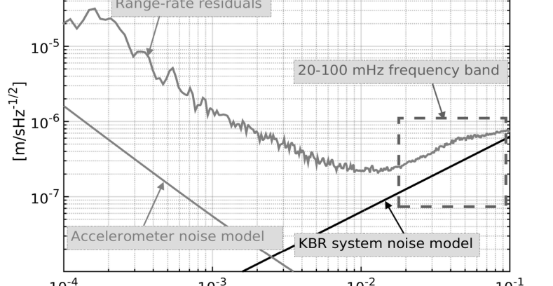
Figure 1: Power spectral density of post-fit range-rate residuals plotted for December 2008 and compared with the prelaunch models of the kbr system noise and the accelerometer noise.

Our contribution focuses on the following points

1. Unidentified effects in the snrs.

2. The analysis of post-fit range-rate residuals with focus on the non-stationary errors in the high frequencies and their contribution to the parameters estimated during the gravity field parameter estimation process.

Our main contribution is the analysis of the post-fit range-rate residuals with focus on the kbr system noise. In order to understand the kbr system noise it is important to understand the snrs of the four frequencies of the kbr microwave ranging system. Therefore, we analyzed the snrs and found that there are effects in snr related to the moon intrusions and magnetic-torquer rod currents. These effects are in addition to those previously identified by Harvey et al. [2016]. First, we present those effects in the snr values and then we present an analysis of the high-frequency spectrum of post-fit range-rate residuals where the k-band ranging system noise is dominating. The outline of our contribution is as follows. We discuss the moon intrusions and magnetic-torquer rod currents in Section 1. Further, we discuss our gravity field parameter estimation scheme in Section 2 followed by an analysis of the post-fit range-rate residuals with focus on the high-frequency errors in Section 2.1. The contribution of the high-frequency errors in the estimated parameters is discussed in Section 2.2.

1 Unidentified effects in the SNRs

The range observations are computed by the combination of k- and ka-band phase observations from the two satellites. In order to investigate the system noise of the grace k-band ranging system, it is important to understand the quality of these four phase observations. The snr values of these observations reflect the signal strength and ranging measurement quality. They are also used to filter the spurious phase measurements when combining the four phase measurements to get the inter-satellite range data. The combination is performed by jpl during the kbr level 1a to level 1b processing. The snr values are expressed as a factor of 0.1db-hz in the standard kbr level 1b data. The phase measurements below snr values 340 0.1db-hz are considered as spurious and are therefore not considered in the combination of phase measurements. This means either we see a gap in the data or interpolated values depending upon the length of the time interval [Wu et al., 2006].
According to Harvey et al. [2016], the snr value is defined as the amount of power in 20 ms integrations of signal power (integrated against a phase locked local model) compared to an integration with the local model in quadrature. The minimum snr requirement for the grace mission is 63 db-hz or 630 0.1db-hz (as given in the standard kbr level 1b data).

The 1-$\sigma$ (1-phase) error corresponding to the snr for 1 s time interval data is given as

$$\sigma^{\text{K/Ka}}_{\phi,i}=\frac{1}{2\pi(\textsc{snr}^{\text{K/Ka}}_{i})}$$ (1)

in units of cycles [Thomas, 1999] where ‘$i$’ $\in\text{\{A, B\}}$. Eqn. 1 demonstrates that low snrs can lead to high noise in the phase observations. The total noise of the phase observations constitutes the k-band ranging system noise (see Thomas [1999] for details), which dominates in high frequencies (above 20 mhz) of the range-rate observations. In order to understand the error characteristics of the range-rate residuals in high frequencies, we therefore need to analyze the snrs of the phase observations. In the following subsections, we present the systematic effects that are not yet discussed in the existing literature.

1.1 Moon intrusion effects on SNR

The grace star cameras are blinded by the sun and the moon every 161 d and 27 d respectively [Bandikova, 2015]. These effects are called sun and moon intrusions. Each spacecraft has two star cameras on board, designated as head#1 and head#2, which are located on the lateral side of each spacecraft. In Fig. 3, the star camera baffle represents the location of one of the star camera heads on that lateral side. During the in-flight attitude control, when one of the star camera heads is blinded, the other head is set as primary star camera, which is available for the attitude determination. When both star camera heads are available, the attitude of the spacecraft is obtained by combining the data of the two star camera heads which is done during the ground processing [Bandikova, 2015, Romans, 2003].

(a.)

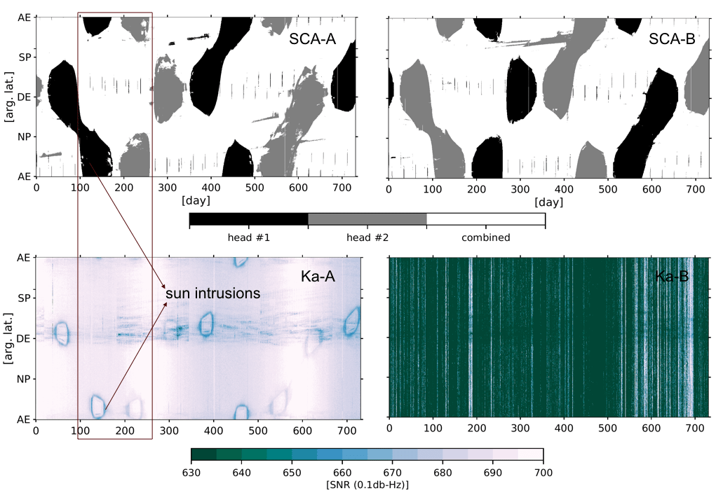
(b.)

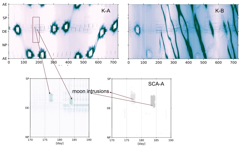
Figure 2: The top row shows when the star camera heads were blinded during the year 2007 and 2008, where gray color and black color represent the blinding of the head#2 and head#1 respectively and white means both star camera heads are available for the attitude determination. The ka-band snrs of grace-a and b are shown in second row and the k-band snrs are shown in third row. The fourth row shows a zoomed-in view of the moon intrusions into snr and blinded heads of star camera of corresponding spacecraft.

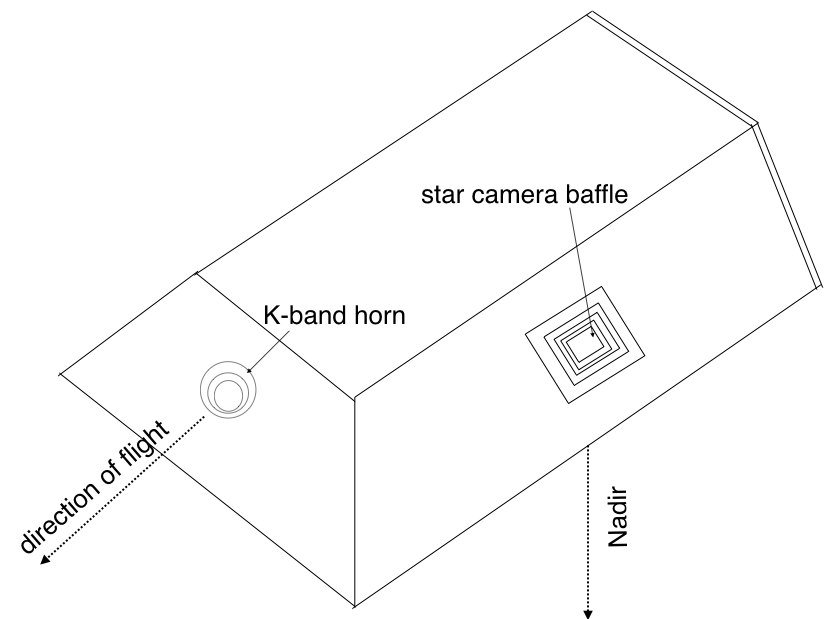
Figure 3: Star camera baffle structure on the grace spacecraft after Harvey et al. [2016].

Fig. 2a (sca-a and sca-b) shows the sun and moon intrusions into the star camera of each satellite during the year 2007 and 2008. Black color represents the periods when head#1 was blinded and head#2 was active, gray color represents the periods when head#2 was blinded and head#1 was active, white color represents the periods when none of the heads were blinded.

As shown in the same figure (cf. Fig. 2), all the three valid snrs (k-b, k-a, ka-a) of both spacecraft experience a drop in their values during the intrusions into the star camera. As previously mentioned, the ka-band snr of grace-b (ka-b) was anomalous during this time and, thus, we do not observe any related characteristics in these values. Here we focus only on the affect of the moon intrusions on the snrs, which are highlighted in the k-band snr of grace-a (Fig. 2, bottom left panel) and the corresponding star camera data flags plotted for the same duration (Fig. 2, bottom right panel). The ka-band snr of grace-a and k-band snr of grace-b also suffered from moon intrusions, but their values did not drop below mission requirements (630 0.1db-hz). The snrs were still ranging between 675-685 0.1db-hz. However, the k-band snr of grace-a dropped much lower (ranging between 630-640 0.1db-hz) than the other two snrs during moon intrusions, sometimes even below mission requirements (for example, moon intrusions between the days 400-500).

Ring shape structure during the moon intrusions in the snrs which we can see in the zoomed-in plot in the bottom panel of Fig. 2(b), are similar to the ring shape structures during the sun intrusions in the snrs. In the bottom panel of Fig. 2(b), moon intrusions are shown in snr during days from 170 to 190. The signatures of moon intrusions resemble the physical structure of the star camera baffle (cf. Fig. 3), similar to the signatures left by sun intrusions.

Since the sun intrusions effects were identified in grace before the launch of grace-follow on (grace-fo), the grace-fo kbr assembly will be shielded to protect it from the interference caused by the instrument processing unit (ipu). Therefore, we do not expect to find the moon intrusion effects on snr in grace-fo data (personal communication, Gerhard L. Kruizinga, jpl, nasa on 10 oct. 2016).

1.2 Magnetic torquer rod current effects on SNR

Three magnetic torquer rods (mtq) located off-center in each grace spacecraft, mounted parallel to the satellite body reference triad, serve as the primary attitude control actuators. Magnetic torquers generate a magnetic dipole m, whose magnitude is dependent on the applied electric current. The resulting torque T acting on the spacecraft is then given as the vector product of the sum of the magnetic dipoles generated by all three mtqs and the earth's magnetic flux density B (cf. Eqn. 2) [Wertz, 1978].

$$\textbf{T}=\textbf{m}\times\textbf{B}$$ (2)

In Fig. 4, the absolute value of the magnetic torquer rod currents of both satellites are plotted along the argument of latitude for the years 2007 and 2008. The variation in the currents every 161 d is dependent on the primary star camera head during attitude determination and the accuracy of the attitude observed by it.

According to Herman et al. [2004], Bandikova [2015], during 2007 and 2008 attitude observed by head#2 was more accurate than that of the attitude observed by head#1 of both spacecraft. When head#2 was used in the attitude control loop, less torque was needed to keep the satellite attitude within the limits required for inter-satellite pointing. Therefore, the electric currents flowing through the mtqs were smaller during the period when head#2 was available. During the period when head#1 was used in the attitude control loop, more electric currents were needed. As a result of the differences between the accuracies of the two star camera heads on board each spacecraft, we see the alternate 161 d period variations in the magnitude of the electric currents flowing through the three rods of each spacecraft (cf. Fig. 4).

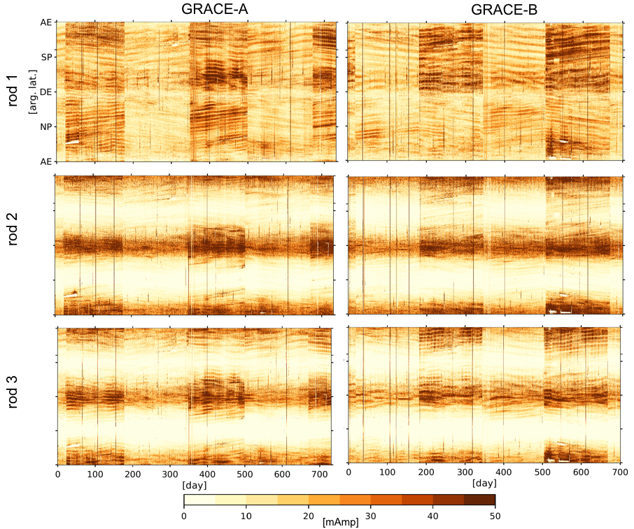
Figure 4: Absolute value of currents in the three magnetic torquer rods of grace-a and grace-b for 2007 and 2008. Periods of 161 days with high currents along the equator (descending and ascending) can also be seen which are related to satellite attitude.

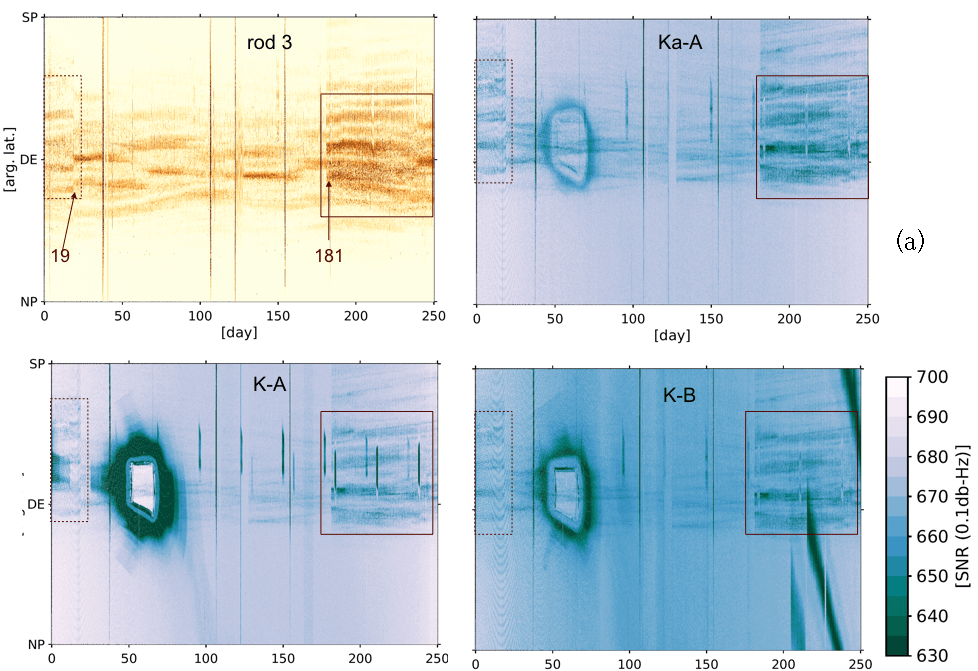
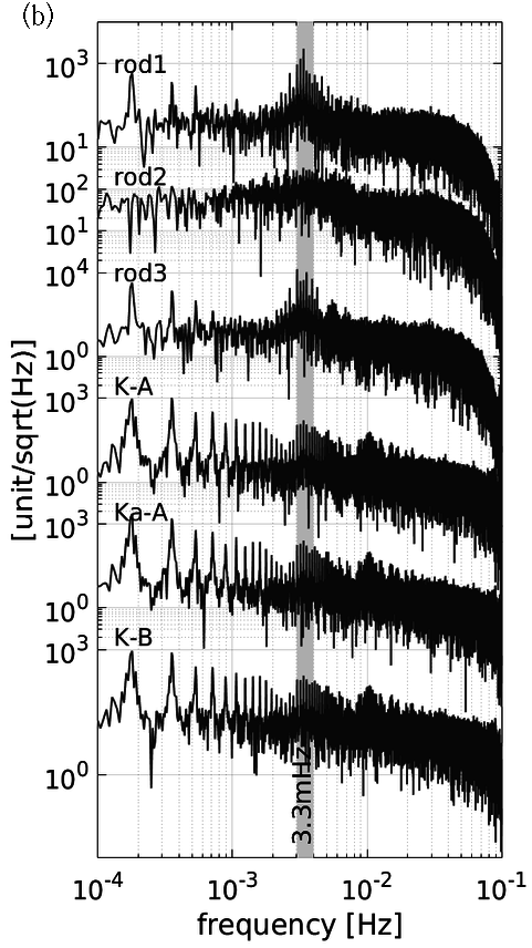
Figure 5: (a) Above: Effects of the currents of rod 3 of grace-b on the three snrs of the kbr microwave system. The effects are shown for 250 days of year 2007 highlighted with the regions with high torquer rod currents and the affected snrs due to them. The color scale of the plotted currents of the rod 3 are same as that of the currents plotted in Fig. 4.
(b) Left: The power spectral densities of the three magnetic torquer rod currents of grace-b and the three snrs (k- and ka-band snr of grace-a and k-band snr of grace-b). All the three snrs also show a peak at the frequency 3.3 mhz which is the dominant frequency of the currents flowing through mtqs.

The three valid snrs, which are ka-band snr of grace-a, k-band snr of grace-a and b, are observed to be affected by the mtqs of grace-b. The three valid snrs of both spacecrafts are found to be correlated with the currents flowing through rod 2 and 3 of grace-b. In Fig. 5(a) we show the correlations present between rod 3 of grace-b and the three valid snrs of both spacecrafts as a zoomed-in picture for the 250 days of year 2007. The currents were smaller between days 19 to 180 as opposed to days from 181 to 250. This is because the primary star camera head from day 19 to day 180 was head#2 and beyond that it was head#1 on grace-b (see Fig. 2 for the details of primary star camera heads). During the period of strong currents (from day 181 to 250) flowing through rod 3 of grace-b, their effect on the snrs can be seen easily in all the three snr plots as opposed to the period when small currents were flowing (from the day 19 to 180) through the torquer rods (see highlighted region in Fig. 5(a)). Here, we see that the currents flowing through the mtqs have an impact on the snrs, which is clearly visible in the snrs in Fig. 5. However, there is no drop observed in the snrs below mission requirements (630 0.1db-hz) during any of the alternate 161 d cycle of currents in mtqs.

The power spectral densities of the three valid snrs show large values around the frequency 3.3 mhz which was already found to be associated with the magnetic torquer rod currents of the grace spacecrafts by Bandikova et al. [2012].

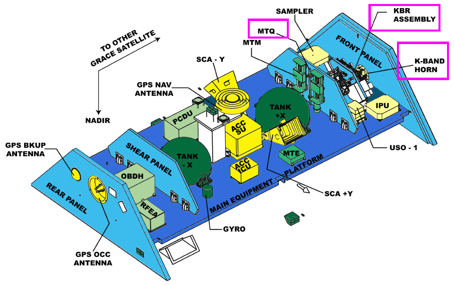
Figure 6: Internal view of grace showing the location of the mtqs near the front panel where kbr assembly is mounted. ⓒ https://directory.eoportal.org/web/eoportal/satellite-missions/g/grace

In Fig. 6, we see that the kbr assembly is located near one of the mtq rods. It is possible that the currents flowing through the rod are causing the electromagnetic interference that affects the kbr assembly. Thus, we see a correlation between the mtq current and variations in the snrs. However, this hypothesis has to be studied further. Investigations related to mtq rod current effects on primary sensors (accelerometer, star-trackers, kbr assembly) are ongoing in jpl, nasa (personal communication, Gerhard L. Kruizinga, 10 oct. 2017).

2 Analysis of the post-fit range-rate residuals

In this section, we discuss the errors absorbed by the high-frequency range-rate residuals $(f>{20}\,\mathrm{m\textsc{h}z})$ and their possible sources. Here, we analyze the range-rate residuals that are obtained after the full parameter estimation chain of the gravity field parameter estimation.

The gravity field parameters are estimated using the standard itsg-2014 processing chain [Mayer-Gürr et al., 2014]. The unconstrained monthly solutions are estimated up to degree 60 using the variational equations approach. For details regarding the implementation of the approach see Mayer-Gürr [2006]. The unknown parameters are estimated using least-squares variance component estimation [Koch & Kusche, 2002]. These unknown parameters include the Stokes’s coefficients, initial orbital state parameters, accelerometer scale and bias parameters. The orbital state ($r$, $\dot{r}$) and the accelerometer parameters are estimated once per day along the three axes (x, y, z).

The basic least-squares adjustment is as follows –

$$\Delta{{l}} =\mbox{\boldmath$\Delta{{\hat{l}}}$}+\mbox{\boldmath$\hat{e}$}_{\text{{kbr}}}+\mbox{\boldmath$\hat{e}$}_{\text{{gps}}}+\mbox{\boldmath$\hat{e}$}_{\text{{acc}}},$$ (3)

$$\Delta{{\hat{l}}} =\mathbf{A}\,\mbox{\boldmath$\Delta{\hat{x}}$}$$ (4)

where, $\mathbf{A}$ is the design matrix of size (i$\times$j), (i, j)$\in$(rows, columns).
$\Delta{\hat{x}}$ consists of estimated Stokes’s coefficients ($\text{c}_{nm}$, $\text{s}_{nm}$), accelerometer scale and bias parameters, and orbital state parameters ($r$, $\dot{r}$).
$\Delta{{l}}$ are the reduced range-rate observations $(\delta{\dot{\rho}})$, gps observations containing satellite state parameters ($r$, $\dot{r}$) and accelerometer scale and bias parameters.
$\mbox{\boldmath$\hat{e}$}_{\text{{kbr}}},\mbox{\boldmath$\hat{e}$}_{\text{{gps}}},\mbox{\boldmath$\hat{e}$}_{\text{{acc}}}$ are the range-rate residuals, orbital state residuals, accelerometer scale and bias residuals respectively.

Reduced range-rate observations $(\delta{\dot{\rho}})$ used in parameter estimation are computed as -

$$\delta{\dot{\rho}} =\dot{\rho}-\dot{\rho}_{0}$$ (5)

where, $\dot{\rho}$ and $\dot{\rho}_{0}$ are the observations obtained from the satellite and observations computed from the dynamic orbit that is obtained from the state-of-the art background models, respectively. Background models used to compute $\dot{\rho}_{0}$ are mentioned in Table 1. We use the term ‘pre-fit range-rate residuals’ for reduced range-rate observations $(\delta{\dot{\rho}})$ and ‘post-fit range-rate residuals’ for the range-rate observations obtained as residuals of the reduced range-rate observations after least-squares parameter estimation fit denoted as ($\mbox{\boldmath$\hat{e}$}_{\textsc{\text{kbr}}}$) in Eqn. 4. In the following sections, we use the notation ($\hat{e}$) to refer to the post-fit residuals of range-rate observations ($\mbox{\boldmath$\hat{e}$}_{\textsc{\text{kbr}}}$).

Table 1: Background models (perturbations) that are reduced from the range-rate observations during gravity field processing.

Models	Standards
Earth rotation	IERS 2010 [Petit & Luzum, 2010]
Moon, sun and planet ephemeris	JPL DE421 [Folkner et al., 2009]
Earth tide	IERS 2010 [Petit & Luzum, 2010]
Ocean tide	EOT11a [Savcenko & Bosch, 2012]
Pole tide	IERS 2010 [Petit & Luzum, 2010]
Ocean pole tide	Desai 2003 [Petit & Luzum, 2010]
Atmospheric tides (S1, S2)	Bode-Biancale 2003 [Bode & Biancale, 2006]
Atmosphere and Ocean Dealiasing	AOD1B RL05 [Flechtner et al., 2015]
Relativistic corrections	IERS 2010 [Petit & Luzum, 2010]
Permanent tidal deformation	includes (zero tide)

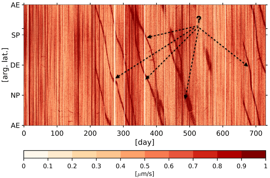
Figure 7: Post-fit range-rate residuals computed using the itsg-2014 parameter estimation chain and are plotted on an absolute scale. The residuals are plotted for the two year duration starting from 1 january 2007.

2.1 Error characteristics of the high-frequency range-rate residuals

This section focuses on understanding of the error characteristics of high-frequency post-fit range-rate residuals ($>$20 mhz) and identifying their sources. As seen in Fig. 7, one of the most interesting features in the post-fit range-rate residuals is the pattern of bands with high value of post-fit residuals, which begins from day 200 and continues until the end of december 2008 (day 730). The structure of these bands changes and repeats after a shift in time.

Here, we are interested in understanding:

• why is the amplitude of residuals high in certain regions which vary over the orbit and time?

• and in which frequencies do these errors lie? It is important to know whether they are affecting the most important frequency band of the large time-variable gravity field signal, i.e., 0.1-18 mhz [Thomas, 1999].

Investigation of the post-fits revealed that these features are dominating in the frequencies above 20 mhz which are plotted in Fig. 8. The filters applied on the post-fit range-rate residuals are provided by Hewitson [2007].

We denote the set of high-pass filtered post-fit range-rate residuals as $(\hat{e}_{\text{HP}})$ and low-pass filtered post-fit range-rate residuals as $(\hat{e}_{\text{LP}})$. The set of low-pass filtered $(<{20}\,\mathrm{m\textsc{h}z})$ post-fit range-rate residuals does not contain these features. Comparison of the two filtered sets of post-fit residuals when plotted on an absolute scale (cf. Fig. 9) shows that the high value of post-fit residuals forming the band shaped pattern is dominating in frequencies above 20 mhz.

In order to find their source, we investigated the four snrs of frequencies of the kbr assembly. Since they are the fundamental entity used to compute the kbr system noise, which is dominating in the frequencies above 20 mhz [Thomas, 1999]. The comparison of the snrs and the high-frequency post-fit residuals show that the bands of high value of residuals are dependent on the variations in the k-band snr of grace-b. The value of post-fit residuals are high in the regions along the orbit where the k-band snr of grace-b drops down to 550 0.1db-hz, which is well below the defined mission requirements. Since no other snr shows these patterns (cf. Fig. 2), the only source of errors in the post-fit residuals responsible for these bands is the degraded signal quality of k-band frequency of grace-b, which is reflected in its snr. As investigated by Harvey et al. [2016], the drops in the k-band snr of grace-b are dependent on the temperature variations observed by one of the thermistors located near microwave assembly. Thus, these band forming patterns of high value of post-fit residuals are due to the temperature effects on the ranging frequencies. As the four phase observations (k- and ka-band of grace-a & b) are combined to form the range-rates [Wu et al., 2006], these errors propagate to the range-rate observations and, consequently to the range-rate residuals.

Another feature which is also present in the high-frequency range-rate residuals $(\hat{e}_{\text{HP}})$ is the signatures related to the sun intrusions into the snrs (cf. Fig. 8(a), (b), (c)). As seen in the Fig. 2, all the valid snrs drop during the sun intrusions into the star cameras. However, one possible source responsible for the sun intrusion dependent errors in the high-frequency residuals is the k-band snr of grace-a as the drop in its value during sun intrusions is larger (down to 550 0.1db-hz) as compared to the snrs of ka- and k-band of grace-a and grace-b respectively. The differences in the effects on snrs are due to differences in the microwave assemblies used in the two grace spacecrafts (for details see Harvey et al. [2016]).

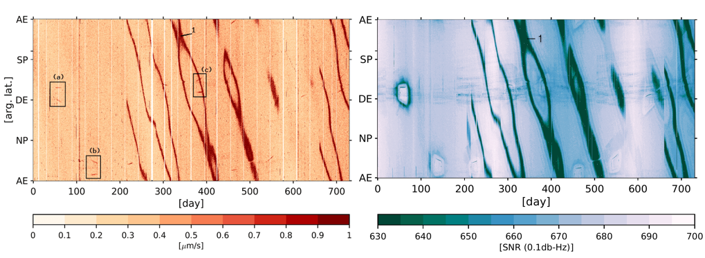
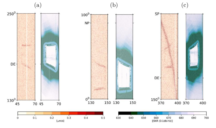
Figure 8: Above: (right) Absolute of the high-frequency post-fit residuals ($\hat{e}_{\text{HP}}$) plotted for year 2007 and 2008 along the argument of latitude and time in days along with the k-band snr of grace-b (left); temperature dependent bands are marked as ‘1’ and ‘(a)’, ‘(b)’, ‘(c)’ are the effects related to the sun intrusions; below: are the zoomed-in picture of the residuals correlated with the sun intrusions related effects in the snrs. The k-band snr of grace-a is plotted here to show the correlation with postfits.

The amplitude of the residuals is high where the k-band snr of grace-a drops in the inner ring structure caused by the sun intrusions as shown in Fig. 8(a), (b), (c) as a zoomed-in plot. However, the signatures of the sun intrusion dependent errors are not as strong as temperature dependent errors in post-fit range-rate residuals. In Fig. 9(a) and (c.), we see that the strength of the intrusion dependent errors in the absolute pre-fit residuals is weaker than the temperature dependent errors. It implies that the range-rate observations are more affected by the temperature effects than by the sun intrusion effects. The amplitude of pre-fit range-rate residuals of August 2008 are comparatively higher than the other months. However, the solution converged with the noise level comparable to other months as can be seen in the post-fit range-rate residuals.

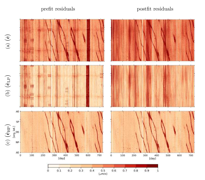
Figure 9: Comparison of the absolute values of pre-fit and post-fit residuals (a) and their low-pass (b) and high-pass filtered parts (c). The darkest patch from the day 578 to 609 shows that the prefits were comparatively higher for the month of August 2008 than the other months. However, the solution converged with the noise level comparable to other months as can be seen in the postfits.

So far, we have shown that the errors in the high frequencies are largely reflected in the post-fit range-rate residuals. However, it is difficult to say that they are completely absorbed by them without leakage of any part of them in to the estimated parameters. Our approach to observe and to quantify this is to compare the differences between the reduced range-rate observations (pre-fit range-rate residuals defined in Section 2) with the post-fit range-rate residuals. The differences should show the amount of the signal mapped on to the parameters estimated (Stokes’s coefficients, orbital state parameters, accelerometer scale and bias). Thus, we analyze their differences in the following section.

2.2 Contribution of high-frequency errors in range-rate observations into the estimated gravity field parameters

In order to investigate whether the investigated high-frequency errors of the range-rate observations are propagated into the estimated parameters, in this section, we analyze the absolute of the differences between the pre-fit and the post-fit residuals. Note that, the estimated parameters include unknown initial positions of the orbit determination problem $\mathbf{(r,\dot{r})}$, scale $\mathbf{({S_{x}},{S_{y}},{S_{z}})}$ and bias of the accelerometer $\mathbf{({b_{x}},{b_{y}},{b_{z}})}$ and Stokes’s coefficients $(\mathbf{c_{nm},s_{nm}})$ (cf. Eqn. 10).

$$\text{Estimated parameters}=\left[\begin{array}[]{c}\mathbf{c_{nm},s_{nm}}\\ \mathbf{(r,\dot{r})}_{i}\\ \mathbf{({S_{x}},{S_{y}},{S_{z}})}_{i}\\ \mathbf{({b_{x}},{b_{y}},{b_{z}})}_{i}\end{array}\right]$$ (10)

where $i\in${A, B}.

The absolute differences between the pre-fit and post-fit residuals should indicate the signal that has been absorbed by the estimated parameters (cf. Eqn. 10). Although the kbr noise is observed in the high-frequency spectrum, we look at the differences between the full signals, their low-frequency ($<$20 mhz) parts as well as the high-frequency parts ($>$20 mhz) altogether in Fig. 10 plotted on an absolute scale.

The differences between the pre-fit and post-fit residuals (cf. Fig. 10 (a.)) show that the contribution of low frequencies into the estimated parameters is significantly higher than the high frequencies. These differences in Fig. 10 (a.) are highly correlated with the differences of the low-pass filtered parts of the post-fit and pre-fit residuals, i.e. Fig. 10 (b.). The range-rate residuals in the low frequencies ($<$20 mhz) are dominated by the attitude errors, accelerometer dependent errors and errors from other unknown sources as discussed in Section Introduction. The analysis of these low-frequency errors in the range-rate residuals is beyond the scope of this paper. The differences of the high-frequency filtered set of residuals plotted on the different color scale (cf. Fig. 10 (c.)) shows the noise that is mapping into the estimated parameters.

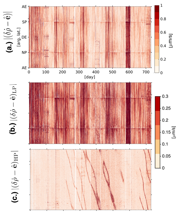
Figure 10: (a.) shows the differences between the pre-fit and post-fit residuals, (b.) shows the low-pass filtered part of the differences between the pre-fit and post-fit residuals and (c.) presents the high-pass filtered part of the differences shown in (a.). All values are plotted on an absolute scale. Their statistical descriptions are defined in the Table 2.

Table 2: Statistical description of the differences shown in Fig. 10, their high-pass filtered and low-filtered parts shown in the same figure.

	Differences	Low-pass filtered	High-pass filtered
	(a.) $(\delta\dot{\rho}-\mathbf{\hat{e}})$	(b.) $(\delta\dot{\rho}-\mathbf{\hat{e}})_{\text{LP}}$	(c.) $(\delta\dot{\rho}-\mathbf{\hat{e}})_{\text{HP}}$
Mean ($\nicefrac{\mathrm{\mu m}}{\mathrm{s}}$)	$0.19654$	$0.19431$	$0.00384$
RMS ($\nicefrac{\mathrm{\mu m}}{\mathrm{s}}$)	$0.662431$	$0.65859$	$0.01926$
Median ($\nicefrac{\mathrm{\mu m}}{\mathrm{s}}$)	$0.124630$	$0.12372$	$0.00183$
Ratio of mean values		$\left|\frac{\text{{(b.)}}}{\text{{(a.)}}}\right|\,=\,0.98865$	$\left|\frac{\text{{(c.)}}}{\text{{(a.)}}}\right|\,=\,0.01957$
Ratio of median values		$0.99276$	$0.01471$

Ratios in the column (c.) of Table 2 explains the amount of high-frequency filtered noise to the total noise mapped into the estimated parameters (cf. Eqn. 10). Similarly, the amount of low-frequency noise mapped in to the estimated parameters is explained in the ratios of column (b.) of Table 2. The ratios are computed for the mean and median values both. The median is more robust to the outliers whereas mean value is less. Hence, we take the both statistical descriptors into account in order to explain the amount of high-frequency filtered noise mapped in to the estimated parameters. In order to compute the ratios, first, we compute the differences between pre-fit and post-fit residuals. Second, we take the low-pass and high-pass filtered parts of the computed differences. Finally, we compute the mean and median of the differences and their low-pass and high-pass filtered parts. The absolute of the mean and median values are presented in the Table 2 . The ratios are computed from the absolute values computed for each i.e. differences of pre-fit and post-fit residuals, their low-pass and high-pass filtered parts.

From the ratios explained in Table 2, it is clear that the contribution of the low-frequency noise to the estimated parameters is significant as compared to the high-frequency noise. Both, ratios of the mean and median values show that the contribution of high-frequency errors is as small as $\approx$ 1 % whereas the contribution of the low-frequency errors is $\approx$ 99 % in to the estimated parameters. However, the contribution of the high-frequency part is reaching up to 30 % of the total error contribution in the months where the temperature dependent non-stationary errors were high (cf. Fig. 10(c.)). Again, it should be kept in mind that this percentage contribution could be distributed to any of the parameters estimated (cf. Eqn. 10) during the gravity field processing.

Since it is clear that the contribution of the high-frequency errors into the estimated parameters is significantly small still, it is worth to model and investigate the impact of these errors on the gravity field solutions in future, once the full understanding of these errors is established.

3 Summary and outlook

Our contribution focused on two parts - In the first part we presented an analysis of the snr of the k-band ranging assembly where we present the effects in the snr that were not known before. In second part, we have shown that the high kbr system noise which leads to the degraded quality of range observations, is responsible for the noise in high-frequency range-rate residuals.

First, we presented results of analysis of the snrs of four frequencies on board grace. The analysis of snrs revealed two more systematic effects which were not known. We presented that the moon intrusions also affect the quality of the snrs (in Section 1.1). The effect of moon intrusions into snrs repeats every 26 d. For most of the duration, the drop in the snr values was not below mission requirements but we show that there are periods when the snr drops significantly even below mission requirements during moon intrusions. Since the kbr assembly of grace-follow on (grace-fo) will be shielded to protect it from electromagnetic interference between ranging frequencies and the instrument processing unit, the identified moon intrusion effects into the star camera are not expected to influence the ranging frequencies in grace-fo (personal communication, Gerhard L. Kruizinga on 10 Oct. 2016).

Further, we presented the source of effects in snrs along the equator which were not explained by Harvey et al. [2016]. The effects are found to be dependent on the varying currents in the mtqs (in Section 1.2). We have shown that the currents in the mtqs of grace-b are affecting all the three valid snrs, i.e. k- and ka-band frequency of grace-a and k-band frequency of grace-b. The snrs also contain the mtqs dominant frequency 3.3 mhz.

One possible reason could be the electromagnetic interference between the magnetic torquer rod currents and the frequencies of the k-band ranging assembly. However, the hypothesis has to be studied further. The investigations related to the magnetic torquer rod currents induced signals on the grace observations are ongoing in the jpl, nasa (personal communication, Gerhard L. Kruizinga on 12 Oct. 2017).

Second, we presented an analysis to study the noise present in high-frequency range-rate observations in Section 2. The quality of the high -frequency range-rate observations is highly affected by the instrument temperature variations and intrusions in the star cameras, which is reflected in terms of degraded snr values. Errors due to the temperature variations and the sun intrusions are well reflected in the range-rate residuals. We have shown in Section 2.2 that a significantly small part of the high-frequency errors is absorbed by the parameters estimated (see Eqn. 10 for the list of estimated parameters) during gravity field parameter estimation.

As we mentioned in Section 1.2 that the investigations are still ongoing in jpl, nasa in order to understand such effects, a model needs to be developed after the establishment of their full understanding. The model and their full understanding are required to investigate their impact on gravity field and also to mitigate such errors during the pre-processing step in grace gravity field modeling.
Considering the grace-follow on (grace-fo), it is difficult to predict the nature of errors which would affect the ranging quality before its launch. However, this study can be used as a basis to investigate the errors in the range-rate residuals and to find their sources in early stage of the mission, in order to benefit from the grace-fo. An understanding of the errors propagating to the range observations during the initial stage of grace-fo can be helpful in many ways, such as – finding the possibility to correct them, for example, by satellite maneuvers, and developing the better data processing strategies or noise modeling approaches to mitigate the propagation of these errors in to the gravity field solutions.

References

- Bandikova et al. [2012] Bandikova T., Flury J. & Ko U.D., Characteristics and accuracies of the GRACE inter-satellite pointing, Advances in Space Research, 50 (2012), pp. 123-135, doi: 10.1016/j.asr.2012.03.011.
- Bandikova & Flury [2014] Bandikova, T. & Flury, J., Improvement of the GRACE star tracker data based on the revision of the combination method, Advances in Space Research, 54 (2014), pp. 1818-1827, doi: 10.1016/j.asr.2014.07.004.
- Bandikova [2015] Bandikova T., Role of attitude determination for inter-satellite pointing, Phd thesis, Leibniz Universität Hannover, Germany (2015), url: https://dgk.badw.de/fileadmin/user_upload/Files/DGK/docs/c-758.pdf.
- Bode & Biancale [2006] Bode A. & Biancale R., Mean Annual and Seasonal Atmospheric Tide Models Based on 3-hourly and 6-hourly ECMWF Surface Pressure Data, (Scientific Technical Report STR06/01), Deutsches GeoForschungsZentrum GFZ, 33 S, doi: 10.2312/GFZ.b103-06011.
- Ditmar et al. [2012] Ditmar P., Teixeira da Encarnação J. & Hashemi Farahani, H., Understanding data noise in gravity field recovery on the basis of inter-satellite ranging measurements acquired by the satellite gravimetry mission GRACE, Journal of Geodesy, 86 (2012), pp. 441-465, doi: 10.1007/s00190-011-0531-6.
- Flechtner et al. [2015] Flechtner F., Dobslaw H. & Fagiolini E., Gravity Recovery and Climate Experiment, AOD1B Product Description Document for Product Release 05, ftp://podaac.jpl.nasa.gov/allData/grace/docs/AOD1B_PDD_v4.4.pdf.
- Folkner et al. [2009] Folkner W.M., Williams J.G. and Boggs H.D., The Planetary and Lunar Ephemeris DE 421, IPN Progress Report 42-178, (2009), https://ipnpr.jpl.nasa.gov/progress_report/42-178/178C.pdf.
- Goswami & Flury [2016a] Goswami S. & Flury J., Identification and separation of GRACE sensor errors in range-rate residuals, GRACE Science Team Meeting, Oct. Potsdam, Germany (2016).
- Goswami & Flury [2016b] Goswami S. & Flury J., Detecting the signatures of sensor-errors in GRACE range-rate residuals, AGU Fall Meeting, San Francisco, US, Dec. (2016), url: http://adsabs.harvard.edu/abs/2016AGUFM.G13A1081G
- Harvey [2016] Harvey N., GRACE star camera noise, Advances in Space Research, 58 (2016), pp. 408-414, doi: 10.1016/j.asr.2016.04.025.
- Harvey et al. [2016] Harvey N., Dunn C., Kruizinga G. & Young L., Triggering Conditions for GRACE Ranging Measurement Signal-to-Noise Ratio Dips, Journal of Spacecraft and Rockets, 54 (2016), pp. 327-330, doi: 10.2514/1.A33578.
- Herman et al. [2004] Herman J., Presti D., Codazzi A. & Belle C., Attitude control for GRACE: the first low-flying satellite formation, In ESA SP-548: 18th International Symposium on Space Flight Dynamics, (2004), url: http://www.issfd.org/ISSFD_2004/papers/P0106.pdf
- Hewitson [2007] Hewitson M., LTPDA, a MATLAB toolbox for accountable and reproducible data analysis, Max-Planck-Institut für Gravitationsphysik, Leibniz Universität Hannover Germany, (2007), url: https://www.elisascience.org/ltpda.
- Petit & Luzum [2010] Petit G. and Luzum B. (eds.)., IERC Conventions (2010), IERS Technical Note No. 36 Frankfurt am Main: Verlag des Bundesamts für Kartographie und Geodäsie, (2010), 179 pp., ISBN 3-89888-989-6, url: https://www.iers.org/IERS/EN/Publications/TechnicalNotes/tn36.html
- Inàcio et al. [2015] Inàcio P., Ditmar P., Klees R. & Farahani H.H., Analysis of star camera errors in GRACE data and their impact on monthly gravity field models, Journal of Geodesy, 89 (2015) pp. 551-571, doi: 10.1007/s00190-015-0797-1.
- Kim [2000] Kim J., Simulation Study of A Low-Low Satellite-to-Satellite Tracking Mission, Phd thesis, Center for Space and Research, Texas, US, (2000), url: http://granite.phys.s.u-tokyo.ac.jp/ando/GRACE/Kim_dissertation.pdf.
- Klinger & Mayer-Gürr [2016] Klinger B. & Mayer-Gürr T., The role of accelerometer data calibration within GRACE gravity field recovery: Results from ITSG-2016, Adv. in Space Res., 58 (2016), pp. 1597-1609, doi: 10.1016/j.asr.2016.08.007.
- Ko [2008] Ko U.D., Analysis of the characteristics of the GRACE dual one way ranging system, Phd thesis, Center for Space and Research, Texas, US, (2008), url: http://hdl.handle.net/2152/17977.
- Ko et al. [2012] Ko U.D., Tapley B., Ries J.C. & Bettadpur S., High-Frequency Noise in the Gravity Recovery and Climate Experiment Intersatellite Ranging System, Journal of Spacecraft and Rockets, 25 (2012), pp. 1163-1173, doi: 10.2514/1.A32141.
- Ko et al. [2015] Ko U.D., Wang F. & Eanes J.R., Improvement of Earth Gravity Field Maps after Pre-processing Upgrade of the GRACE Satellite‘s Star Trackers, The Korean Society of Remote Sensing, 31 (2015), pp.353-360, url: http://www.koreascience.or.kr/article/ArticleFullRecord.jsp?cn=OGCSBN_2015_v31n4_353.
- Koch & Kusche [2002] Koch, KR. & Kusche, J., Regularization of geopotential determination from satellite data by variance components, Journal of Geodesy, 76 (2002), pp. 259-268, doi: 10.1007/s00190-002-0245-x
- Mayer-Gürr [2006] Mayer-Gürr T., Gravitationsfeldbestimmung aus der analyse kurzer bahnbögen am beispiel der satellitenmissionen CHAMP und GRACE, PhD Thesis, Institut für Theoretische Geodäsie der Universität Bonn, Germany, (2006), url: http://hss.ulb.uni-bonn.de/2006/0904/0904.pdf.
- Mayer-Gürr et al. [2014] Mayer-Gürr T., Klinger B., Zehentner N. & Kvas A., ITSG-GRACE 2014, Oct., GRACE Science Team Meeting, Potsdam, Germany, (2014), url: https://www.tugraz.at/institute/ifg/downloads/gravity-field-models/itsg-grace2014/.
- Meyer et al. [2016] Meyer U., Jäggi A., Jean Y. & Beutler G., AIUB-RL02: an improved time-series of monthly gravity fields from GRACE data, Geophysical Journal International, 205 (2016), pp. 1196–1207, doi: 10.1093/gji/ggw081.
- Montenbruck & Gill [2000] Montenbruck O. & Gill E., Satellite Orbits - Models, Methods and Applications, Springer-Verlag Berlin Heidelberg, XI, 369, ISBN:978-3-642-58351-3, 2002.
- Ramillien, Frappart & Seoane [2014] Ramillien G. Frappart F. & Seoane L., Application of the Regional Water Mass Variations from GRACE Satellite Gravimetry to Large-Scale Water Management in Africa, Remote Sens., 6 (2014), pp. 7379-7405, doi: 10.3390/rs6087379.
- Romans [2003] Romans L., Optimal combination of quaternions from multiple star cameras, May, JPL, NASA, (2003), ftp://podaac.jpl.nasa.gov/allData/grace/docs/quaternion_memo.pdf.
- Savcenko & Bosch [2012] Savcenko R. & Bosch W., EOT11a - empirical ocean tide model from multi-mission satellite altimetry, DGFI Report No. 89, http://epic-reports.awi.de/36001/1/DGFI_Report_89.pdf.
- Siemes et al. [2013] Siemes, C., Ditmar, P., Riva, R.E.M. et al., Estimation of mass change trends in the Earth’s system on the basis of GRACE satellite data, with application to Greenland, Journal of Geodesy, (2013), 87:69, doi: 10.1007/s00190-012-0580-5.
- Tapley et al. [2004] Tapley B.D., Bettadpur S., Watkins M. & Reigber C., The gravity recovery and climate experiment: Mission overview and early results, Geophys. Res. Lett., 31 (2004), L09607, doi: 10.1029/2004GL019920.
- Thomas [1999] Thomas J.B., An analysis of Gravity-field estimation based on inter-satellite dual-1-way biased ranging, JPL Publication 98-15, (1999), ftp://podaac.jpl.nasa.gov/allData/grace/docs/JPL_PUB_98-15.pdf.
- Wertz [1978] Wertz James R., Spacecraft Attitude Determination and Control, 1978, Springer Netherlands, ISBN:978-94-009-9907-7.
- Wu et al. [2006] Wu S.C., Kruizinga G. & Bertiger W., Algorithm Theoretical Basis Document for GRACE Level-1B Data Processing V1.2, Tech. Rep. JPL D-27672, Jet Propulsion Laboratory, (2006), ftp://podaac.jpl.nasa.gov/allData/grace/docs/ATBD_L1B_v1.2.pdf.
- Yang et al. [2013] Yang J.,Gong P., Fu R. et al., The role of satellite remote sensing in climate change studies, Nature Clim. Change, 3 (2013), doi: 10.1038/nclimate1908.