Effects of Interactions on Dynamic Correlations of Hard-Core Bosons at Finite Temperatures

Abstract

We investigate how dynamic correlations of hard-core bosonic excitation at finite temperature are affected by additional interactions besides the hard-core repulsion which prevents them from occupying the same site. We focus especially on dimerized spin systems, where these additional interactions between the elementary excitations, triplons, lead to the formation of bound states, relevant for the correct description of scattering processes. In order to include these effects quantitatively we extend the previously developed Brückner approach to include also nearest-neighbor (NN) and next-nearest neighbor (NNN) interactions correctly in a low-temperature expansion. This leads to the extension of the scalar Bethe-Salpeter equation to a matrix-valued equation. Exemplarily, we consider the Heisenberg spin ladder to illustrate the significance of the additional interactions on the spectral functions at finite temperature which are proportional to inelastic neutron scattering rates.

I Introduction

Computing dynamic correlations in spin systems is one of the main tasks in order to understand the physics in real quantum magnets. Many exotic ground states without long-range order, for instance spin liquids, can be identified in neutron scattering experiments by their specific excitation spectra Balents (2010). From an experimental point of view, thermal fluctuations often smear out the characteristic signatures in momentum and frequency space making clear statements difficult Paddison et al. (2017). This calls for theoretical predictions extended to finite temperatures in order to directly compare with experiments. This goal, however, often proves challenging because at finite temperatures the full trace over the Hilbert space has to be taken into account, i.e., the complete Hilbert space contributes. Especially interactions between excitations can change the energy landscape significantly by means of bound states or long-range entanglement.

Recently it was shown, that the Heisenberg ladder with strong inter-rung frustration is such an extreme case Honecker et al. (2016). This model exhibits bound states of the elementary triplon excitations which exist even below the single-triplon gap. Interestingly, these bound states are hidden in the observables accessible by inelastic neutron scattering at zero temperature. At finite temperatures, however, the bound states acquire finite weight and can even dominate the spectrum. Thus, the low-energy physics is best described by strongly interacting and entangled triplons. This analysis shows that the interactions between the elementary excitations can play a crucial role in the dynamics of spin systems at finite temperature.

On the methodical side, there exists a variety of methods to compute the dynamical response of a spin system at finite temperatures Fabricius et al. (1997); Mikeska and Luckmann (2006); Essler and Konik (2008); James et al. (2008); Essler and Konik (2009); Goetze et al. (2010); Exius et al. (2010); Lake et al. (2013); Jensen et al. (2014); Tiegel et al. (2014); Becker et al. (2017). In previous studies Fauseweh et al. (2014); Fauseweh and Uhrig (2015), we established an analytical method to calculate correlation functions at finite temperature based on the Brückner approach, first introduced in nuclear physics and later transferred to solid state physics Kotov et al. (1998). It was gauged against exact data obtained from the Jordan-Wigner mapping to interaction-free fermions Fauseweh et al. (2014). In contrast to most previous studies, the Brückner approach has the asset that it is not restricted to one dimension or small system size, but in return it relies on a small parameter, namely $\exp(-\beta\Delta)$ where $\beta$ is the inverse temperature and $\Delta$ the energy gap, so that it is particularly reliable at low temperatures. It is important to dispose of methods which are applicable for all dimensions because the thermal broadening of hard-core bosonic line shapes is observed also in three dimensions Quintero-Castro et al. (2012). A good description has been obtained by an expansion in the inverse coordination number Jensen et al. (2014). This approach, however, is not justified in low dimensions. So the Brückner approach is the only one which is conceptually applicable in arbitrary dimension.

The basic idea is to expand the single-particle Green function in terms of interaction diagrams and to keep only those diagrams which contribute in leading non-trivial order, i.e., in $\exp(-\beta\Delta)$. These are the ladder diagrams in the self-energy of the single-particle propagator. For gapped spin systems local excitations generically obey a hard-core constraint due to the limited size of the local Hilbert space. In order to be able to apply bosonic perturbation theory this hard-core constraint is incorporated as on-site infinite repulsion $U\to\infty$. The Brückner approach was applied to quantitatively explain the experimental data for two one-dimensional (1D) materials Klyushina et al. (2016); Fauseweh et al. (2016). It was also applied to predict such data in a two-dimensional (2D) material Streib and Kopietz (2015).

So far, only the hard-core repulsion was taken into account in calculations of the low-temperature spectral functions based on the Brückner approach. Omnipresent additional interactions were included only on a mean-field level Streib and Kopietz (2015); Klyushina et al. (2016); Fauseweh et al. (2016). This appeared justified by the dominating strength of the diverging on-site repulsion in comparison to the additional finite interactions. If, however, the additional interactions lead to a significant restructuring of the energy landscape, see discussion of binding phenomena above, a mean-field treatment is no longer justifiable. It is the main focus of this paper to solve this issue.

We derive how the Brückner approach can be extended in order to include additional interactions summing all ladder diagrams. The extended approach correctly captures all scattering processes of two given particles including the formation of bound states. The extension leads to a natural generalization of the scalar Bethe-Salpeter equation for the scattering amplitude to a matrix-valued Bethe-Salpeter equation for the scattering matrix.

As a testbed, we investigate the correlations at finite temperature for Heisenberg spin ladders. These systems feature triplons as elementary excitations which form bound and antibound states in the two-particle sector due to additional interactions. We investigate how these additional interactions influence the single-triplon spectral function at finite temperature. This paves the way to compute correlation functions in more complicated models and thus to explore the interplay of quantum interactions and thermal fluctuations in a broader sense.

The article is set up as follows: In Sect. II, we introduce the hard-core boson model and the parametrization for the additional interaction. In Sect. III, we extend the Brückner approach to additional interactions for hard-core bosons of a single kind, i.e., for the single-flavor case. In Sect. IV an analysis of the approach for the Heisenberg ladder follows, for which we extend it to several flavors as well. We conclude our article in Sect. V.

II Model

Here we introduce the general hard-core boson model and discuss some of its properties. We consider a model with a single kind of boson per site, i.e., a single flavor, in order to keep the notation transparent. This setting can be extended later on to several flavors. The Hamiltonian of the system reads

$$H_{0} =E_{0}+\sum\limits_{i,d}\left(h_{d}b_{i}^{\dagger}b_{i+d}^{\phantom{\dagger}}+\mathrm{h.c.}\right)$$

$$+\sum\limits_{i,d_{1},d_{2},d_{3}}V_{d_{1},d_{2},d_{3}}b_{i}^{\dagger}b_{i+d_{1}}^{\dagger}b_{i+d_{1}+d_{2}}^{\phantom{\dagger}}b_{i+d_{3}}^{\phantom{\dagger}}+\dots,$$ (1)

where $E_{0}$ is the ground state energy, $i,d,d_{1},d_{2},d_{3}$ are site indices and $b_{i,\alpha}^{\dagger},b_{i,\alpha}$ are the hard-core bosonic creation and annihilation operators. We describe the approach for the one-dimensional case explicitly, but all definitions and equations can be implement straightforwardly in higher dimensions as well. The dispersion of the excitations is given by the Fourier sum of the hopping matrix elements $h_{d}$. We assume that the model has an energy gap $\Delta$ between the ground state and the minimum of the single-particle band. The general two-particle interaction is described in real space by the matrix elements $V_{d_{1},d_{2},d_{3}}$. Interactions among more particles, for example genuine three-particle interactions, are shown as dots in (II) and can appear in the model, but are neglected in our approximation.

We assume that the Hamiltonian $H_{0}$ describes the hopping and interaction of conserved particles, i.e., the number of particles (hard-core bosons) does not change. In general, a microscopic Hamiltonian will not have this property, for instance if it is derived from a spin model Sachdev and Bhatt (1990). But one can map such microscopic non-conserving Hamilton operators to effective Hamilton operators which conserve the particle number. There exists a variety of methods in literature which can be used to obtain such an effective Hamiltonian from a general Hamiltonian Sólyom (1979); Metzner et al. (2012); Wegner (1994); Głazek and Wilson (1993, 1994); Knetter and Uhrig (2000); Knetter et al. (2003a); Kehrein (2006); Fischer et al. (2010); Fauseweh and Uhrig (2013); Shastry and Sutherland (1981); Uhrig et al. (1999); Haegeman et al. (2013); Keim and Uhrig (2015); Vanderstraeten et al. (2015). Hence, here, we do not consider this step, but rather discuss the general properties of (II).

Figure 1: Diagrammatic representation of the interaction vertex in Eq. (II)

Transforming the interaction into momentum space yields the interaction vertex including the on-site hard-core repulsion $U$

$$V(p,k,q) =\frac{U}{N}$$

$$+\frac{1}{N}\sum\limits_{d_{1},d_{2},d_{3}}V_{d_{1},d_{2},d_{3}}e^{-id_{2}p}e^{-id_{1}k}e^{id_{3}q},$$ (2)

where $U$ is taken later to infinity to implement the hard-core property. The corresponding diagram is represented in Fig. 1. We stress that the additional interactions, i.e., all terms proportional to $V$, in Eq. (II) will depend on the momenta $k$ and $q$. Defining the momentum dependent vector

$$\mathbf{f}^{\dagger}(k)=(1,e^{ik},e^{-ik},e^{i2k},e^{-2ik},\cdots),$$ (3)

we can rewrite the interaction vertex as a bilinear form

$$V(p,k,q)=\frac{1}{N}\mathbf{f}^{\dagger}(k)\underline{\underline{\Gamma}}_{0}(p)\mathbf{f}(q).$$ (4)

The advantage of this notation is that the dependencies on the momenta $p,k$, and $q$ are factorized. The first few entries of the matrix $\underline{\underline{\Gamma}}_{0}(p)$ read

$$\underline{\underline{\Gamma}}_{0}(p) =$$ (5a)

$$\begin{pmatrix}U&0&0&\cdots\\ 0&\sum\limits_{d_{2}}V_{1,d_{2},1}e^{-id_{2}p}&\sum\limits_{d_{2}}V_{1,d_{2},-1}e^{-id_{2}p}&\cdots\\ 0&\sum\limits_{d_{2}}V_{-1,d_{2},1}e^{-id_{2}p}&\sum\limits_{d_{2}}V_{-1,d_{2},-1}e^{-id_{2}p}&\cdots\\ \vdots&\vdots&\vdots&\ddots\end{pmatrix}$$

$$=:\underbrace{\begin{pmatrix}U&0&\cdots\\ 0&0&\cdots\\ \vdots&\vdots&\ddots\end{pmatrix}}_{\underline{\underline{U}}}+\underline{\underline{V}},$$ (5b)

where $\underline{\underline{U}}$ and $\underline{\underline{V}}$ are block matrices acting on different subspaces.

Below, we investigate the single-particle spectral function of the hard-core bosons defined by

$$A(p,\omega)=\frac{-\mathrm{Im}}{\pi\sqrt{L}}\lim_{i\omega_{\nu}\rightarrow\omega+i0^{+}}\int_{0}^{\beta}\mathrm{d}\tau e^{i\omega_{\nu}\tau}\sum_{j}e^{-ipj}G(j,\tau),$$ (6)

where $G(j,\tau)$ is the single-particle temperature Green function

$$G(j,\tau)=-\left\langle T\left\{b_{j}^{\dagger}(-i\tau)b_{0}^{\phantom{\dagger}}(0)\right\}\right\rangle.$$ (7)

and $L$ the system size. The Matsubara frequencies are denoted by $\omega_{\nu}=2\nu\pi/\beta$ where $\beta=1/T$ is the inverse temperature setting the Boltzmann constant to unity. The spectral function is connected to the dynamic structure factor by means of the fluctuation-dissipation theorem

$$S(p,\omega)=\frac{1}{1-e^{-\beta\omega}}\left[A(p,\omega)+A(p,-\omega)\right],$$ (8)

which is directly accessible in inelastic neutron scattering experiments.

III Brückner approach

In this section, we show how additional interactions can be included within the Brückner approach. To keep the presentation transparent we describe the procedure for a single flavor of hard-core bosons per site. In App. A we show how the approach can be extended to include multi-flavored bosons such as triplons in dimerized spin systems.

The Brückner approach is a low-temperature approximation for the single-particle spectral function based on diagrammatic perturbation theory. The key idea is to replace the hard-core bosonic creation and annihilation operators by normal bosonic operators and to enforce the hard-core constraint by an on-site repulsion $U$ which is taken to infinity in the end. The expansion parameter of the theory is the low density of excitations which is given proportional to $\exp(-\beta\Delta)$.

In leading order, all diagrams with a single propagator running backwards in imaginary time must be included. This leads to the summation of ladder diagrams as shown in Fig. 2. Here we extend the previous approach Fauseweh et al. (2014); Fauseweh and Uhrig (2015); Streib and Kopietz (2015) by including also the additional interaction matrix elements $V_{d_{1},d_{2},d_{3}}$ in the diagrammatic ladders. In this way, we can explore how the additional interactions affect the single-particle properties.

Figure 2: Ladder diagrams with the interaction vertex given in Eq. (II).

Figure 3: Graphical definition of the scattering amplitude $\Gamma$.

In a first step, we calculate the scattering amplitude $\Gamma$ as defined graphically in Fig. 3. The scattering amplitude describes the complete scattering of two particles. It can be found as solution of the Bethe-Salpeter equation depicted in Fig. 4 and denoted explicitly

$$\Gamma(P,K,Q) =\frac{V(p,k,q)}{\beta}$$ (9)

$$-\frac{1}{\beta}\sum\limits_{L}\Gamma(P,K,L)G(P+L)G(-L)V(p,l,q).$$

The capital letters are shorthand for the momentum and the Matsubara frequency, e.g., $P=(p,i\omega_{p})$. We stress that due to the additional interactions $\Gamma$ also depends on the relative momenta $K$ and $Q$, making the integration more challenging.

Figure 4: Bethe-Salpeter equation for the ladder diagrams in Fig. 3.

Since the dependence of the elementary interaction vertex $V(p,k,q)$ on the momenta factorizes, we apply the same ansatz to the scattering amplitude

$$\Gamma(P,K,Q)=\frac{1}{N}\mathbf{f}^{\dagger}(k)\underline{\underline{\Gamma}}(P)\mathbf{f}(q)$$ (10)

which implicitly defines the scattering matrix $\underline{\underline{\Gamma}}(P)$. Inserting Eqs. (4) and (10) into Eq. (9) and separating the dependence on the momenta yields

$$\underline{\underline{\Gamma}}(P) =\underline{\underline{\Gamma}}_{0}(p)$$ (11)

$$-\frac{1}{N\beta}\sum\limits_{L}\underline{\underline{\Gamma}}(P)G(P+L)G(-L)\mathbf{f}(l)\mathbf{f}^{\dagger}(l)\underline{\underline{\Gamma}}_{0}(p).$$

This equation is the generalization of the scalar Bethe-Salpeter equation for the scattering amplitude to the matrix-valued Bethe-Salpeter equation for the scattering matrix $\underline{\underline{\Gamma}}(P)$. In addition, we also define the matrix

$$\underline{\underline{N}}(P):=\frac{1}{N}\sum\limits_{l}\mathbf{f}(l)\mathbf{f}^{\dagger}(l)M(P,l),$$ (12)

where we used the scalar function

$$M(P,l) :=\frac{1}{\beta}\sum\limits_{i\omega_{l}}G(P+L)G(-L).$$ (13)

Since the frequency dependence of $M(P,l)$ is in $\mathcal{O}(\omega_{p}^{-1})$, the matrix $\underline{\underline{N}}(P)$ has a spectral Hilbert representation. We denote its spectral function by $\underline{\underline{\rho}}(p,\omega)$. Inserting the previous definitions into the Bethe-Salpeter equation (9) yields the matrix expression

$$\underline{\underline{\Gamma}}(P)=\underline{\underline{\Gamma}}_{0}(p)-\underline{\underline{\Gamma}}(P)\underline{\underline{N}}(P)\underline{\underline{\Gamma}}_{0}(p),$$ (14)

which represents a geometric series for matrices. It can be easily solved by the scattering matrix

$$\underline{\underline{\Gamma}}(P) =\left(\underline{\underline{\Gamma}}_{0}^{-1}(p)+\underline{\underline{N}}(P)\right)^{-1}.$$ (15)

In analogy to the scalar case Fauseweh et al. (2014) the spectral representation of $\underline{\underline{\Gamma}}(P)$ has two contributions: (i) A high-energy contribution stemming from a virtual antibound state at $\omega\approx U$ and (ii) a low-energy contribution, where $\omega\approx\Delta$. In the following two subsections we will determine the exact form of these contributions taking the additional interaction into account.

III.1 High-energy contribution

The aim is to perform the limit $U\to\infty$ analytically. At low energies, one can set $U=\infty$ in the equations and evaluate them straightforwardly. But there also arise contributions from an antibound state at high energies. The analytical determination of these contributions required some care for the on-site repulsion. Due to the additional interaction, these contributions are modified as we explain now.

To compute the exact contribution we need to calculate the position of the pole in the spectral representation of $\underline{\underline{\Gamma}}(P)$ for $\omega\approx U$. The pole can be obtained from the zero eigen value of the matrix inverse of Eq. (15)

$$\underline{\underline{\Gamma}}(P)^{-1}=\underline{\underline{\Gamma}}_{0}^{-1}(p)+\underline{\underline{N}}(P).$$ (16)

Note, that

$$\underline{\underline{\Gamma}}_{0}^{-1}(p)=\underline{\underline{U}}^{-1}+\underline{\underline{V}}^{-1}$$ (17)

holds where it is understood that the matrix inverses of $\underline{\underline{U}}$ and $\underline{\underline{V}}$ are in the respective subblocks where the matrices contribute, see Eq. (5b). This means that $\underline{\underline{U}}^{-1}$ only has an entry in the $(1,1)$ matrix element, and $\underline{\underline{V}}^{-1}$ only for matrix elements $(m,n)$ with $m,n>1$.

If we expand $\underline{\underline{N}}(P)$ for $\omega\rightarrow\infty$ we obtain

$$\underline{\underline{N}}(P)=\frac{\underline{\underline{\rho}}_{0}(p)}{\omega}+\frac{\underline{\underline{\rho}}_{1}(p)}{\omega^{2}}+\mathcal{O}\left(\frac{1}{\omega^{3}}\right),$$ (18)

where $\underline{\underline{\rho}}_{m}(p)$ denotes the $m^{\mathrm{th}}$ moment in $x$ of the matrix-valued spectral function $\underline{\underline{\rho}}(p,x)$. This is in complete analogy to the scalar case in Refs. Fauseweh et al. (2014); Fauseweh and Uhrig (2015), but generalized here to matrices.

We introduce the parametrization $\omega=\bar{\omega}U$, such that $\bar{\omega}=\mathcal{O}(1)$ for $U\to\infty$. Inserting the expansion of $\underline{\underline{N}}(P)$ into Eq. (16) yields

$$\underline{\underline{U}}^{-1}+\underline{\underline{V}}^{-1}+\frac{1}{U\bar{\omega}}\underline{\underline{\rho}}_{0}(p)+\frac{1}{U^{2}\bar{\omega}^{2}}\underline{\underline{\rho}}_{1}(p)$$ (19)

$$=\underline{\underline{V}}^{-1}+\frac{1}{U}\underbrace{\left(\frac{1}{\bar{\omega}}\underline{\underline{\rho}}_{0}(p)+U\underline{\underline{U}}^{-1}\right)}_{X_{1}}+\frac{1}{U^{2}}\underbrace{\left(\frac{\underline{\underline{\rho}}_{1}(p)}{\bar{\omega}^{2}}\right)}_{X_{2}}.$$

To determine the correct contribution from the antibound state at frequencies $\omega\approx U$, we need to calculate the scattering matrix in this frequency range. For this purpose, we employ matrix perturbation theory in the parameter $1/U$. The zeroth order is given by $\underline{\underline{V}}^{-1}$. The perturbations are the matrices $X_{1}$ and $X_{2}$ in first and second order, respectively. We denote by $(\lambda_{i},\mathbf{e}_{i})$ the unperturbed eigen pair, i.e., eigen value and corresponding eigen vector, of $\underline{\underline{V}}^{-1}$. The first eigen pair represents the important contribution of the antibound state and reads

$$\lambda_{1}=0\,,\quad\mathbf{e}_{1}=(1,0,0,\dots)^{\mathrm{T}}.$$ (20)

But for any finite $U$, higher order contributions mix into this eigen pair. We refer the reader to App. B for the discussion of the matrix perturbation theory which is essentially standard first and second order perturbation theory from any quantum mechanics text book.

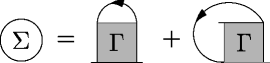
Figure 5: Self-energy diagrams obtained from summing the scattering matrix $\Gamma(P,K,Q)$ with another dressed propagator.

Once the scattering matrix has been calculated, the self-energy contribution from the antibound state at high energy (denoted ‘he’) can be calculated by closing the scattering matrix by another propagator, see arrowed propagator in Fig. 5. The first diagram on the right hand side in Fig. 5 corresponds to the Hartree contribution and the second to the Fock contribution. Explicitly, they are given by

$$\Sigma_{\mathrm{he}}(P)=$$ (21)

$$\sum\limits_{K}G(K)\left[\Gamma(P+K,-P,-P)+\Gamma(P+K,-K,-P)\right].$$

The explicit sum over the Matsubara frequencies is similar to the one in the scalar case Fauseweh et al. (2014); Fauseweh and Uhrig (2015). Inserting the expression for the scattering amplitude yields for the Hartree contribution

$$\Sigma_{\mathrm{Hart,he}}(P)=-\frac{1}{N}\sum\limits_{k}\int\limits_{-\infty}^{\infty}\mathrm{d}x^{\prime}\frac{A_{k}(x^{\prime})U^{2}\rho^{11}_{0}(p+k)\left[1-\frac{1}{U}\sum\limits_{j\neq 1}\frac{1}{\rho_{0}^{11}(p+k)}2\mathrm{Re}\left(W_{j}(p+k)^{*}f_{j}(-p)\right)\right]}{i\omega_{p}-(\omega_{U}(p+k)-x^{\prime})}\frac{1}{e^{\beta x^{\prime}}-1}.$$ (22)

where the functions $W_{j}$ (and $V_{j}$ for later use), $f_{j}$ and $\omega_{U}$ are defined in App. B. The Hartree and Fock contribution of the pure hard-core repulsion reads

$$\Sigma_{\mathrm{Hart},U}=\Sigma_{\mathrm{Fock},U}=\frac{1}{N}\sum\limits_{k}\int\limits_{-\infty}^{\infty}\mathrm{d}x^{\prime}A_{k}(x^{\prime})U\frac{1}{e^{\beta x^{\prime}}-1}.$$ (23)

Expanding the high energy Hartree term in $1/U$ and combining it with $\Sigma_{\mathrm{Hart},U}$ of the pure hard-core repulsion we eventually perform the limit $U\to\infty$ and obtain

$$\Sigma_{\mathrm{Hart,he}}(P)+\Sigma_{\mathrm{Hart},U}=-\frac{1}{N}\sum\limits_{k}\int\limits_{-\infty}^{\infty}\mathrm{d}x^{\prime}A_{k}(x^{\prime})\left[\frac{-i\omega_{p}}{\rho^{11}_{0}(p+k)}-\frac{\sum\limits_{i\neq 1}V_{i}(p+k)}{{\rho^{11}_{0}}^{2}(p+k)}\right.$$ (24)

$$\left.-\frac{\rho^{11}_{1}(p+k)}{{\rho_{0}^{11}}^{2}(p+k)}+\frac{x^{\prime}}{\rho^{11}_{0}(p+k)}-\sum\limits_{j\neq 1}\frac{1}{\rho_{0}^{11}(p+k)}2\mathrm{Re}\left(W_{j}(p+k)^{*}f_{j}(-p)\right)\right]\frac{1}{e^{\beta x^{\prime}}-1}.$$

Note that this results directly reflects the relevant expression for the hard-core particles.

The Fock term can be computed in a similar fashion yielding

$$\Sigma_{\mathrm{Fock,he}}(P)+\Sigma_{\mathrm{Fock},U}=-\frac{1}{N}\sum\limits_{k}\int\limits_{-\infty}^{\infty}\mathrm{d}x^{\prime}\frac{A_{k}(x^{\prime})}{e^{\beta x^{\prime}}-1}\left[\frac{-i\omega_{p}}{\rho^{11}_{0}(p+k)}-\frac{\sum\limits_{i\neq 1}V_{i}(p+k)}{{\rho^{11}_{0}}^{2}(p+k)}\right.$$ (25)

$$\left.-\frac{\rho^{11}_{1}(p+k)}{{\rho_{0}^{11}}^{2}(p+k)}+\frac{x^{\prime}}{\rho^{11}_{0}(p+k)}-\sum\limits_{j\neq 1}\frac{1}{\rho_{0}^{11}(p+k)}\left(W_{j}(p+k)^{*}f_{j}(-p)+W_{j}(p+k)f_{j}(-k)^{*}\right)\right].$$

Comparing these expressions to the ones in the case of a pure hard-core repulsion, see Eq. (A7) in Ref. Fauseweh et al., 2014, we see that two additional contributions to the real part of the self-energy arise from the additional interactions.

III.2 Low-energy contribution

In the low-energy sector, we can take the limit $U\rightarrow\infty$ directly without considering intricate limits. Then, the matrix $\underline{\underline{\Gamma_{0}}}^{-1}$ equals $\underline{\underline{V}}^{-1}$. We use the Hilbert representation of $\underline{\underline{N}}$ to calculate the Hilbert representation of $\underline{\underline{\Gamma}}(P)-\underline{\underline{V}}(p)$, i.e., the ladder diagrams minus the simple Hartree-Fock diagrams which are constant in frequency

$$\underline{\underline{\Gamma}}(P)-\underline{\underline{V}}(p) =\int\limits_{-\infty}^{\infty}\mathrm{d}x^{\prime}\frac{\underline{\underline{\rho}}_{\Gamma}(p,x^{\prime})}{i\omega_{p}-x^{\prime}},$$ (26a)

$$\underline{\underline{\rho}}_{\Gamma}(p,\omega) =\begin{pmatrix}\rho^{11}_{\Gamma}&\rho^{12}_{\Gamma}&\cdots\\ \rho^{21}_{\Gamma}&\rho^{22}_{\Gamma}&\cdots\\ \vdots&\vdots&\ddots\end{pmatrix}$$ (26b)

$$=\frac{-\mathrm{Im}}{\pi}\lim\limits_{i\omega_{p}\rightarrow\omega}\left(\underline{\underline{V}}^{-1}+\underline{\underline{N}}(P)\right)^{-1}-\underline{\underline{V}}.$$ (26c)

In general, these expressions cannot be simplified further analytically. For a given interaction, however, the spectral representation can be obtained numerically for fixed frequency and momentum.

Next, we determine the low-energy (le) contributions to the self-energy. Similar to the high-energy contributions, there are Hartree- and the Fock-like contributions which result from the two ways to close the scattering amplitude, see Fig. 5.

They appear in the two terms in

$$\Sigma_{\mathrm{le}}(P) =\sum\limits_{K}G(K)(\Gamma(P+K,-P,-P)+\Gamma(P+K,-K,-P))$$ (27a)

$$=\frac{-1}{N\beta}\sum\limits_{k,i\omega_{k}}\int\limits_{-\infty}^{\infty}\int\limits_{-\infty}^{\infty}\mathrm{d}x^{\prime}\mathrm{d}x^{\prime\prime}\frac{A_{k}(x^{\prime})}{i\omega_{k}-x^{\prime}}\left(\mathbf{f}^{\dagger}(-p)+\mathbf{f}^{\dagger}(-k)\right)\frac{\underline{\underline{\rho}}_{\Gamma}(p+k,x^{\prime\prime})}{i\omega_{p}+i\omega_{k}-x^{\prime\prime}}\mathbf{f}\left(-p\right),$$ (27b)

The first term represents the Hartree contribution and the second the Fock contribution of the scattering amplitude. We substitute $k\rightarrow k-p$ and sum over all Matsubara frequencies in order to obtain

$$\Sigma_{\mathrm{le}}(P) =\frac{1}{N}\sum\limits_{k}\int\limits_{-\infty}^{\infty}\mathrm{d}x^{\prime\prime}\left[\mathbf{f}^{\dagger}\left(-p\right)+\mathbf{f}^{\dagger}\left(-(k-p)\right)\right]A_{k-p}(x^{\prime\prime}-\omega)\underline{\underline{\rho}}_{\Gamma}(k,x^{\prime\prime})\mathbf{f}\left(-p\right)\left[\frac{1}{e^{\beta(x^{\prime\prime}-\omega)}-1}-\frac{1}{e^{\beta x^{\prime\prime}}-1}\right].$$ (28)

III.3 Hartree-Fock contributions for additional interactions

We stress that the simple Hartree- and Fock-contributions without any frequency dependence cannot be expressed by spectral representations. Hence they must be dealt with separately. For the additional interaction the simple Hartree-term reads

$$\Sigma_{\mathrm{Hart},V} =-\sum\limits_{k}\int\limits_{-\infty}^{\infty}\mathrm{d}x^{\prime}\frac{A_{k}(x^{\prime})}{e^{\beta x^{\prime}}-1}V(p+k,-p,-p).$$ (29)

The Fock-term for the additional interaction is given by

$$\Sigma_{\mathrm{Fock},V} =-\sum\limits_{k}\int\limits_{-\infty}^{\infty}\mathrm{d}x^{\prime}\frac{A_{k}(x^{\prime})}{e^{\beta x^{\prime}}-1}V(p+k,-k,-p).$$ (30)

In the multi-flavor case, the Hartree contribution is multiplied by the number of flavors $N_{\mathrm{f}}$.

III.4 Self-energy and spectral function

Now we are in the position to sum all contributions to the self-energy in leading order in $\exp(-\beta\Delta)$

$$\Sigma =\Sigma_{\mathrm{le}}+\Sigma_{\mathrm{Fock},V}+\Sigma_{\mathrm{Hart},V}+\Sigma_{\mathrm{Fock,he}}$$ (31)

$$+\Sigma_{\mathrm{Fock},U}+\Sigma_{\mathrm{Hart,he}}+\Sigma_{\mathrm{Hart},U}.$$

We omitted the dependence on the total momentum and frequency $P$ for the sake of brevity. The only terms which are not affected by the additional interaction are the simple Hartree- and Fock-Terms $\Sigma_{\mathrm{Hart},U}+\Sigma_{\mathrm{Fock},U}$ of the pure hard-core repulsion. All other contributions include terms which are proportional to $V_{d_{1},d_{2},d_{3}}$.

Once the self-energy is calculated we can determine the spectral function using the Dyson equation

$$A(p,\omega)=$$

$$\quad\frac{-1}{\pi}\frac{\mathrm{Im}\Sigma(\omega,p)}{\left(\omega-\omega(p)-\mathrm{Re}\Sigma(\omega,p)\right)^{2}+\left(\mathrm{Im}\Sigma(\omega,p)\right)^{2}}.$$ (32)

We point out that we sum the diagrams self-consistently, i.e., all propagators are dressed propagators. In practice, we start from an initial guess for the propagators, compute the self-energy, insert it in the Dyson equation (III.4) to determine the propagators. This cycle is iterated as long as the ensuing propagators differ sizeably from the input propagators . As a numerical criteria we use the first and second moment of the spectral function. Once they do not change anymore within machine precision the iteration is stopped and the result is considered to be converged for practical purposes.

IV Results for Heisenberg spin ladders

In this section, we apply the developed Brückner approach including additional interactions to a generic system, namely the dimerized Heisenberg spin $S=1/2$ ladder. It is well established that the elementary excitations in this system are hard-core bosons with three flavors of triplet character Knetter et al. (2001) called triplons Schmidt and Uhrig (2003). At zero temperature, much is known about the system Schmidt and Uhrig (2005) and the agreement between experiment and theory is quantitative Windt et al. (2001); Notbohm et al. (2007). Hence, it is confirmed that the effective Hamiltonian describing the motion and the interaction of the elementary triplons is known, in particular the additional NN and NNN interactions Krull et al. (2012).

In order to illustrate the applicability and usefulness of the extended Brückner approach, we analyze the influence of these additional interactions on the spectral functions of the spin ladder at finite temperatures. This offers the opportunity to explore the feedback effect of strong correlations in the two-particle sector on the single-particle mode at finite temperature.

IV.1 Model of the Heisenberg spin ladder

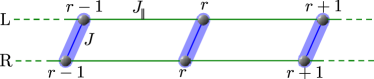
Figure 6: Exchange couplings in the dimerized Heisenberg ladder.

The Hamiltonian of the Heisenberg spin ladder is illustrated in Fig. 6. Its explicit form expressed in spin operators reads

$$H=\sum\limits_{r}J\mathbf{S}_{r}^{\mathrm{L}}\cdot\mathbf{S}_{r}^{\mathrm{R}}+J_{\parallel}\left(\mathbf{S}_{r}^{\mathrm{R}}\cdot\mathbf{S}_{r+1}^{\mathrm{R}}+\mathbf{S}_{r}^{\mathrm{L}}\cdot\mathbf{S}_{r+1}^{\mathrm{L}}\right),$$ (33)

where $J$ is the coupling on the strong bonds on the rungs defining the dimers and $x=J_{\parallel}/J$ is the relative strength of the interdimer coupling along the legs of the ladder. The index $r$ denotes the dimer sites, and L and R refer to the left and right leg of the ladder respectively.

It was shown in Ref. Krull et al. (2012) that deepCUT provides an excellent renormalization tool to compute the effective model in terms of triplons for gapped dimerized spin systems which conserve the triplon number. Thus we use a deepCUT calculation to obtain the hopping and interaction matrix elements of the triplons. The resulting effective Hamiltonian in terms of triplon creation and annihilation operators reads

$$\frac{H_{\mathrm{eff}}}{J} =E_{0}+H_{1}+H_{2}$$ (34)

where $E_{0}$ is the ground state energy, $H_{1}$ the one-triplon Hamiltonian, and $H_{2}$ the two-triplon interaction. The one-triplon Hamiltonian describes the motion of triplons via hopping processes over distance $d$

$$H_{1} =\sum_{r,\alpha}h_{0}t_{r,\alpha}^{\dagger}t_{r,\alpha}^{\phantom{\dagger}}+\sum_{r,|d|>0}\sum_{\alpha}\frac{h_{d}}{2}t_{r+d,\alpha}^{\dagger}t_{r,\alpha}^{\phantom{\dagger}},$$ (35)

where $\alpha\in\left\{x,y,z\right\}$ is the flavor index and $t_{r,\alpha}^{\dagger},t_{r,\alpha}$ are triplon creation and annihilation operators, respectively. Note that we let all triplons hop in the same way due to spin rotation invariance and inversion symmetry fixes $h_{d}=h_{-d}$ being real. The ensuing dispersion $\omega(k)$ reads

$$\omega(k) =\sum_{d\geq 0}h_{d}\cos(dk),$$ (36)

where we set the lattice constant to unity. In this paper, we restrict the hopping range to $|d|\leq 6$ for simplicity. This is completely sufficient to describe the dispersion of spin ladders to good accuracy up to $x=1$.

The two-triplon Hamiltonian describes the additional interactions which are the focus of our work. We restrict them to the processes which can arise up to order 2 in $x$, see Tab. III in Ref. Krull et al., 2012

$$H_{2} =w_{1}\sum_{r}\sum_{\alpha}t_{r,\alpha}^{\dagger}t_{r+1,\alpha}^{\dagger}t_{r+1,\alpha}^{\phantom{\dagger}}t_{r,\alpha}^{\phantom{\dagger}}$$ (37a)

$$+w_{2}\sum_{r}\sum_{\alpha}t_{r+2,\alpha}^{\dagger}t_{r+1,\alpha}^{\dagger}t_{r+1,\alpha}^{\phantom{\dagger}}t_{r,\alpha}^{\phantom{\dagger}}+\mathrm{h.c.}$$ (37b)

$$+w_{3}\sum_{r}\sum_{\alpha\neq\gamma}t_{r,\alpha}^{\dagger}t_{r+1,\alpha}^{\dagger}t_{r+1,\gamma}^{\phantom{\dagger}}t_{r,\gamma}^{\phantom{\dagger}}$$ (37c)

$$+w_{4}\sum_{r}\sum_{\alpha\neq\gamma}t_{r,\alpha}^{\dagger}t_{r+1,\gamma}^{\dagger}t_{r+1,\alpha}^{\phantom{\dagger}}t_{r,\gamma}^{\phantom{\dagger}}$$ (37d)

$$+w_{5}\sum_{r}\sum_{\alpha\neq\gamma}t_{r+2,\gamma}^{\dagger}t_{r+1,\alpha}^{\dagger}t_{r+1,\alpha}^{\phantom{\dagger}}t_{r,\gamma}^{\phantom{\dagger}}+\mathrm{h.c.}$$ (37e)

$$+w_{6}\sum_{r}\sum_{\alpha\neq\gamma}t_{r,\gamma}^{\dagger}t_{r+1,\alpha}^{\dagger}t_{r+1,\alpha}^{\phantom{\dagger}}t_{r,\gamma}^{\phantom{\dagger}}$$ (37f)

$$+w_{7}\sum_{r}\sum_{\alpha\neq\gamma}t_{r+2,\gamma}^{\dagger}t_{r+1,\gamma}^{\dagger}t_{r+1,\alpha}^{\phantom{\dagger}}t_{r,\alpha}^{\phantom{\dagger}}+\mathrm{h.c.}$$ (37g)

We stress that the numerical prefactors $w_{j}$ are determined by a deepCUT calculation of order 6. The precise numbers used are listed in Tab. 1 for the values of $x$ considered in this article.

$x$	$h_{0}$	$h_{1}$	$h_{2}$	$h_{3}$	$h_{4}$	$h_{5}$	$h_{6}$
$0.2$	$1.032449982$	$0.197447202$	$-0.011976902$	$0.001148659$	$-0.000146837$	$0.000021155$	$-0.000003167$
$0.6$	$1.279046995$	$0.508412978$	$-0.131238627$	$0.025917844$	$-0.009368954$	$0.003760173$	$-0.001417178$
$0.8$	$1.447703192$	$0.591395735$	$-0.235167175$	$0.048815082$	$-0.021795289$	$0.010694648$	$-0.004713291$
$1.0$	$1.627729418$	$0.643483774$	$-0.352625277$	$0.075238493$	$-0.037946270$	$0.021098310$	$-0.010197167$

$x$	$w_{1}$	$w_{2}$	$w_{3}$	$w_{4}$	$w_{5}$	$w_{6}$	$w_{7}$
$0.2$	$-0.010542152$	$0.011321380$	$-0.094559805$	$0.099997195$	$0.005991517$	$-0.015979524$	$0.005378499$
$0.6$	$-0.063956523$	$0.103995401$	$-0.249703472$	$0.299185869$	$0.066627091$	$-0.113405271$	$0.044179934$
$0.8$	$-0.071899966$	$0.168824957$	$-0.315550868$	$0.397077500$	$0.120736262$	$-0.153387044$	$0.068217261$
$1.0$	$-0.066366893$	$0.235731322$	$-0.376683724$	$0.492295270$	$0.182036845$	$-0.182288001$	$0.092018083$

Table 1: Upper table: Numerical values of the hopping matrix elements $h_{d}$, see Eq. (35), for various coupling ratios $x=J_{\parallel}/J$ determined by deepCUT. Lower table: Numerical values of the interaction matrix elements $w_{j}$, see Eq. (37), for various coupling ratios $x=J_{\parallel}/J$ determined by deepCUT.

To include the additional interactions among multi-flavored hard-core bosons, we must deal with two types of interaction vertices: (i) ingoing triplons with flavor $\gamma$ and outgoing triplons with flavor $\alpha$ which may or may not be equal to $\alpha$. The value of the interaction vertex depends on $\alpha\neq\gamma$ or $\alpha=\gamma$. (ii) Two triplons with flavor $\alpha\neq\gamma$ go in and come out, i.e., they interact with each other. In the first case, Hartree- and Fock-like diagrams contribute to the self-energy. In the second case, only Hartree-like diagrams contribute. Their contribution acquires a prefactor of $2$ due to the fact that there are two possible flavors for the Green function in the closed loop. Hence, we need two types of interaction matrices: $\underline{\underline{V}}^{\alpha\alpha\gamma\gamma}$ for the type (i) interactions and $\underline{\underline{V}}^{\alpha\gamma\alpha\gamma}$ for the type (ii) interactions.

In our approach we include additional interaction of the form occurring in second order in $x$. This determines the type of quartic terms shown in (37); their prefactors are determined by deepCUT so that higher order contributions are included as well. The terms occurring in (37) have at maximum a spatial range of 2, i.e., besides the rung $r$ the farthest rung addressed is $r\pm 2$. This implies that the matrices $\underline{\underline{\Gamma}}_{0}(p)$ and $\underline{\underline{\Gamma}}(P)$ are finite and can be treated numerically.

Among the ladder diagrams for the self-energy we can distinguish three different types: (a) Fock-like diagrams with interaction matrix $\underline{\underline{U}}+\underline{\underline{V}}^{\alpha\alpha\gamma\gamma}$, (b) Hartree-like diagrams with interaction matrix $\underline{\underline{U}}+\underline{\underline{V}}^{\alpha\alpha\gamma\gamma}$, and (c) Hartree-like diagrams with the interaction matrix $\underline{\underline{U}}+\underline{\underline{V}}^{\alpha\gamma\alpha\gamma}$. In the latter case, $\alpha\neq\gamma$ is implied. The diagrams (a) and (b) can be treated in the same way in the Bethe-Salpter equation, but yield different contributions on the level of the self-energy due to the different final sum over the last propagator (arrow in Fig. 5).

IV.2 Results

The most striking effect of the additional interactions is the occurrence of bound and antibound states in the low-energy sector Uhrig and Schulz (1996, 1998); Trebst et al. (2000); Knetter et al. (2001); Zheng et al. (2001). These states appear because the additional interactions imply either an attractive or repulsive net effect depending on the total spin $S_{\mathrm{tot}}$ of the pair of triplons under study. For $S_{\mathrm{tot}}=0$, rather strong attraction is at work, for $S_{\mathrm{tot}}=1$ it is weaker by about a factor 2 and for $S_{\mathrm{tot}}=2$ the triplons repel each other. Effects of this binding and antibinding can be observed in the matrix elements of $\underline{\underline{\Gamma}}$. In Fig. 7 we show a matrix element of the spectral function $\underline{\underline{\rho}}_{\Gamma}^{xyxy}$.

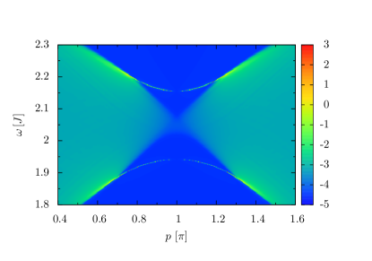
Figure 7: Diagonal (2,2) matrix element of the spectral function $\underline{\underline{\rho}}_{\Gamma}^{xyxy}$ of the scattering matrix for $x=0.2$ at $T=0.3J$ as function of total momentum $p$ and frequency $\omega$. The color axis has a logarithmic scale to depict both strong peaks and weak continua. The arcs below and above the continua around $p=\pi$ stem from the triplet bound state and the quintuplet antibound state, respectively. The singlet bound state does not appear in this spectral response because it does not have overlap with the $xy$ triplon pair.

The spectral function is dominated by a two-particle continuum with a bound state below the continuum and an antibound state above the continuum at $p\approx\pi$. The bound and antibound states coincide with $S_{\mathrm{tot}}=1$ and $S_{\mathrm{tot}}=2$ excitations in the triplon language Zheng et al. (2001); Knetter et al. (2003b). Note, that the $S_{\mathrm{tot}}=0$ bound state does not show up because it has no overlap with the interaction matrix $\underline{\underline{V}}^{\alpha\gamma\alpha\gamma}$ for $\alpha\neq\gamma$.

Next, we investigate the spectral function $A(p,\omega)$ proportional to the scattering rate of inelastic neutron scattering for finite temperatures and various values of the relative coupling strength $x$. Our focus lies on an exemplary comparison of three kinds of results. The first kind is the calculation for a pure hard-core bosonic system, i.e., only the infinite on-site repulsion is taken into account. Its curves are denoted by ‘hard-core’ in the following figures. The second kind is a calculation including the additional interactions on the level of a static Hartree-Fock mean-field calculation as done previously for spin systems Streib and Kopietz (2015); Klyushina et al. (2016); Fauseweh et al. (2016). Its curves are denoted by ‘mean field’ in the following figures. The third kind is the full calculation of the ladder diagrams considering all interaction vertices including those of the additional interactions. Its curves are denoted by ‘full Brückner’ in the following figures.

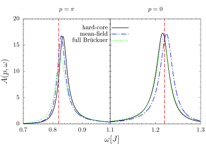
Figure 8: Spectral functions of for $x=0.2$ at momentum $p=\pi$ (left panels, gap mode) and $p=0$ (right panels, maximum mode). The temperature is $T=0.3J$. The vertical dashed lines show where the $T=0$ $\delta$-peaks of the hard-core bosons are located.

Fig. 8 starts the analysis by displaying the spectral functions for $x=0.2$, i.e., the model for which Fig. 7 depicts the signatures of (anti)bound states in the spectral functions of the scattering matrix. Note that the spin ladder has its gap mode, i.e., the mode with the lowest energy at momentum $p=\pi$ while its maximum mode, i.e., the mode with maximum energy, occurs at $p=0$ except for large values of $x\gtrapprox 0.8$. The left panels display the gap modes while the right panels display the mode at $p=0$. The differences between the three kinds of calculations are still fairly small at $x=0.2$ as one might have expected due to the smallness of the corrections. In particular, the broadening is clearly dominated by the scattering due to the hard-core repulsion. It must be noted, however, that the size of the interaction relative to the band width does not vanish for $x\to 0$, but stays finite. Interestingly, even the qualitative position of the peak relative to the $T=0$ dispersion depends on the kind of calculation. The maximum mode (right panel in Fig. 8) in the hard-core calculation lies below the zero-temperature energy, but above it in the mean-field calculation while the full Brückner calculation brings it back to the hard-core calculation.

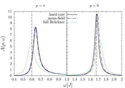
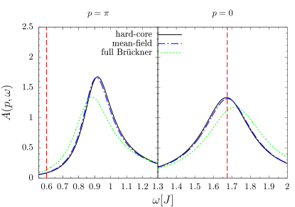
Figure 9: Spectral functions of for $x=0.6$ at momentum $p=\pi$ (left panels, gap mode) and $p=0$ (right panels, maximum mode). The temperature is $T=0.3J$ for the upper panels and $T=0.6J$ for the lower ones. The vertical dashed lines show where the $T=0$ $\delta$-peaks of the hard-core bosons are located.

In order to make the effects more sizeable we pass to larger values of $x$ in Fig. 9 displaying the results for $x=0.6$. Note the changes of scale on the axes relative to Fig. 8. Still, in the panels of Fig. 9 it is clear that the main broadening of the line shapes is due to the hard-core repulsion. This is especially true for larger temperatures where the broadening is rather large growing exponentially $\propto\exp(-\beta\Delta)$ Essler and Konik (2008); James et al. (2008); Essler and Konik (2009); Goetze et al. (2010); Fauseweh et al. (2014); Fauseweh and Uhrig (2015). with temperature in the low-temperature regime. Noticeable in Fig. 9 is the tiny effects of the pure mean-field corrections to the hard-core calculation. Simple frequency-independent Hartree- and Fock-corrections only influence the dispersion a bit and shift the positions of the line shapes. The resulting curves are very close to the pure hard-core line shapes, especially at higher temperatures where the lines are rather broad anyway.

The main observation is that the inclusion of the additional interactions enhance the broadening. Thus the peaks become lower because they become broader. This is rather striking at the lower temperature ($T=0.3J$) where the peak are still very high and prominent. At the higher temperature ($T=0.6J$) the effect is less obvious because the peak width due to hard-core repulsion is already large.

A second noticeable effect of the additional interactions is a shift in the peaks. While the additional broadening was plausibly expected because the additional interactions open additional decay channels the shifts come as a surprise. The gap mode is shifted to lower energies while the maximum mode is shifted to higher energies. Thus, these shifts counteract the tendency induced by the hard-core repulsion of band narrowing, i.e., the lower modes are shifted to higher energies and vice-versa. At low temperatures, the band narrowing is even inverted because the gap mode stays at its $T=0$ while the maximum mode moves a bit upward. At higher temperatures, however, the main effect remains an upward shift of the gap mode although it is slightly reduced by the effects of the additional interactions.

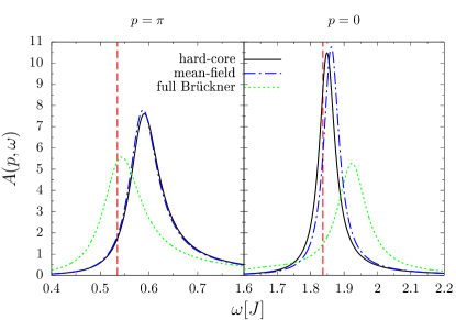
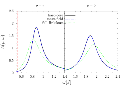
Figure 10: Spectral functions of for $x=0.8$ at momentum $p=\pi$ (left panels, gap mode) and $p=0$ (right panels). The temperature is $T=0.3J$ for the upper panels and $T=0.6J$ for the lower ones. The vertical dashed lines show where the $T=0$ $\delta$-peaks of the hard-core bosons are located.

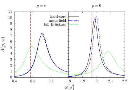
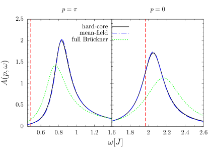
Figure 11: Spectral functions of for $x=1.0$ at momentum $p=\pi$ (left panels, gap mode) and $p=0$ (right panels). The temperature is $T=0.3J$ for the upper panels and $T=0.6J$ for the lower ones. The vertical dashed lines show where the $T=0$ $\delta$-peaks of the hard-core bosons are located.

These observations become more pronounced the stronger the additional interactions are. This is corroborated by data for increasing values of $x$ as depicted in Fig. 10 and Fig. 11. Roughly, the broadening and the shifts increase with increasing $x$, but the effect is not proportional to $x$; the increase is less than linear. We attribute this behavior to the fact that the dominating effect in broadening and shift still is engendered by the hard-core repulsion which is the same in all three cases. Moreover, the band width also increases with $x$ which limits the relative strength of the additional interactions.

At higher temperatures, the strong broadening induced by the hard-core repulsion smears out the line shapes so that the effects of additional interactions become less and less important. This is reasonable because in the limit of infinite temperature only the size of the local Hilbert space matters for the dynamics of the system. Although we are technically working with bosons having infinite-size local Hilbert space the hard-core constraint implemented in the Brückner approach prevents double and higher particle number occupation. Thus, the difference between the pure hard-core calculation and the calculation including additional interactions decreases for higher temperatures.

These observations explain why already the hard-core repulsion describes experimental data very well Klyushina et al. (2016); Fauseweh et al. (2016). Interestingly, the shifts stemming from the additional interactions will improve the agreement between the diagrammatic approach and the peak positions computed numerically by density-matrix renormalization, see Supplemental Material of Ref. Klyushina et al., 2016. We note that the band narrowing Cavadini et al. (2000); Rüegg et al. (2005); Mikeska and Luckmann (2006); Essler and Konik (2008); James et al. (2008); Essler and Konik (2009); Goetze et al. (2010); Tennant et al. (2012); Quintero-Castro et al. (2012) is reduced at high temperatures and even inverted at lower temperatures. This calls for comprehensive further studies in theory and in experiment.

V Conclusions

The goal of this article was to study how additional interactions (besides the hard-core repulsion) in generic hard-core bosonic systems affect the dynamical correlations at finite temperature. To this end, we had to make methodical progress because the diagrammatic Brückner approach formulated so far in solid state physics did not include all interactions, but only the infinite on-site repulsion.

We extended the diagrammatic Brückner approach by including the complete interaction in the summation of all ladder diagrams. The solution of the extended Bethe-Salpeter equation was possible by introducing a scattering matrix which took over the role of the scattering amplitude in the previous case of the pure on-site repulsion. The result describes all possible iterated scattering processes between two given elementary excitations. This allowed us to carry out the intricate limiting procedure $U\to\infty$ analytically. In this way, it was possible to calculate the single-particle self-energy correctly in first order in the expansion parameter $\exp(-\beta\Delta)$. Thus, we perform a systematic expansion valid for low temperatures. The contributions to the self-energy stemming from the virtual antibound state as well as from the low-energy sector due to the additional interactions were derived explicitly.

In order to demonstrate how the method works and to illustrate the importance of the additional interactions we applied the method to a well-understood system with established hard-core bosonic excitations, namely the Heisenberg spin ladder. Here, the elementary excitation are excited spin dimers on the rungs of the ladder including their dressing on the rungs in the vicinity. Due to their total spin $S=1$ they are called triplons and realize hard-core bosons with three flavors corresponding to the three states of a triplet. The effective model at zero temperature expressed in triplon creation and annihilation operators is available for instance by continuous unitary transformations.

At finite temperatures, we compared the line shapes resulting from pure hard-core scattering, from hard-core scattering complemented by mean-field corrections, and from the full Brückner approach. We showed that the dominating effect is the broadening of the $T=0$ $\delta$-peak by the hard-core scattering at finite temperature. The mean-field corrections provide only small modifications. They induce small, almost negligible shifts in the peak positions. The additional interactions, however, have noticeable effects. They induce signatures of bound and antibound states in the spectral functions of the scattering matrix. These are not directly detectable, but the effects on the spectral functions are clear. The additional interactions broaden the lines further since they provide additional decay channels. Concomitantly, they induce certain shifts in the peak positions. Interestingly, these counteract the shifts induced by the hard-core repulsion. The latter imply a certain band narrowing pushing low-lying modes upwards in energy and high-lying ones downward. So the inclusion of the additional interactions reduce this effect of band narrowing and may even invert it for low temperatures. These additional shifts are likely to improve the agreement with experimental observations further.

As an outlook, we point out that besides the single-particle response, multi-particle response can play a significant role in real experiments. The leading effect is given by the broadening induced in the single-particle propagators which carries over to the multi-particle response. Villain pointed out Villain (1975) that for thermal excitations intraband transitions with arbitrary small energy differences are possible leading to a low-energy response at $\omega\approx 0$. This mechanism was discussed and analyzed by Essler and co-workers for the alternating spin chain and the spin ladder in the limit of strong coupling on the dimers and rungs, respectively James et al. (2008); Goetze et al. (2010). At zero temperature, the intraband response completely vanishes because no triplons are thermally excited. Once the temperature is finite, the quasi-particle band is populated and intraband transitions become possible, inducing a finite spectral weight of the low-energy response. In terms of the effective model, such intraband transitions can appear if the corresponding observable includes terms proportional to $t^{\dagger}t$ which is generically the case. Thus the intraband transitions can be interpreted as the propagation of a quasi-particle and an annihilated thermal quasi-particle. Therefore, in first order in $\exp(-\beta\Delta)$, the response at low energies can be calculated by the convolution of single-particle propagators obtained within the Brückner approach. A quantitative discussion is beyond the scope of the present paper, but subject of future research.

Summarizing, the main effect results from the hard-core repulsion as was to be expected from the size of the matrix elements (here $U\to\infty$). But for quantitative analyses, the effect of additional interactions is indeed very important and cannot be neglected. The attempt to take them into account on the mean-field level does not capture the relevant size of the shifts and fails to capture the additional broadening. These insights have only become possible due to the methodical extension of the Brückner approach from pure on-site interaction to general interactions of finite range. The so far scalar geometric series at the basis of the solution of the Bethe-Salpeter equation had to be promoted to a matrix-valued geometric series. Clearly, the application to a wide range of gapped systems is possible. In particular, we emphasize that the Brückner approach can be applied in any dimension.

Appendix A Bosons with multiple flavors

In case of multi-flavored bosons, the most general two-particle interaction is parameterized by

$$V =\sum\limits_{j}\sum\limits_{d_{1},d_{2},d_{3}}\sum\limits_{\alpha,\beta,\gamma,\delta}V^{\alpha\beta\gamma\delta}_{d_{1},d_{2},d_{3}}b^{\dagger}_{j,\alpha}b^{\dagger}_{j+d_{1},\beta}b^{\phantom{\dagger]}}_{j+d_{2},\gamma}b^{\phantom{\dagger}}_{j+d_{2}+d_{3},\delta},$$ (38)

where $d_{1},d_{2},d_{3}\in\mathbb{Z}$ and $d_{1}\neq 0$ and $d_{3}\neq 0$ holds due to the hard-core constraint. The flavor indices are given by $\alpha,\beta,\gamma,\delta$. In momentum space the interaction reads

$$V=\frac{1}{N}\sum\limits_{p,k,q}\sum\limits_{d_{1},d_{2},d_{3}}\sum\limits_{\alpha,\beta,\gamma,\delta}V^{\alpha\beta\gamma\delta}_{d_{1},d_{2},d_{3}}b^{\dagger}_{p+k,\alpha}b^{\dagger}_{-k,\beta}b^{\phantom{\dagger]}}_{p+q,\gamma}b^{\phantom{\dagger}}_{-q,\delta}\cdot e^{-id_{2}p}e^{-id_{1}k}e^{id_{3}q}$$ (39)

The interaction vertex in case of flavored bosons reads

$$V^{\alpha\beta\gamma\delta}(p,k,q)=\frac{U}{N}+\frac{1}{N}\sum\limits_{d_{1},d_{2},d_{3}}V^{\alpha\beta\gamma\delta}_{d_{1},d_{2},d_{3}}e^{-id_{2}p}e^{-id_{1}k}e^{id_{3}q}.$$ (40)

The corresponding diagram is represented in Fig. 12.

Figure 12: Diagrammatic representation of Eq. (40) for multi-flavored bosons.

In the Heisenberg ladder, two kinds of interactions of the hard-core triplons are present: $V^{\alpha\alpha\gamma\gamma}$ for interactions with the same flavor for the ingoing triplons and the same flavor for the outgoing triplons and $V^{\alpha\gamma\alpha\gamma}$ for the interaction of bosons with different flavors. Hence, we will focus our analysis on this special case.

The main change in comparison to the single-flavor case is that the scattering matrix also acquires flavor indices, which represent super indices. As a result, the matrix dimension for $\underline{\underline{\Gamma}}$ scales with the squared number of flavors $N_{\mathrm{f}}^{2}$. First, we solve the Bethe-Salpeter equation for the case $V^{\alpha\alpha\gamma\gamma}$

$$\underline{\underline{\Gamma}}^{\alpha\alpha\gamma\gamma}(P) =\left({\underline{\underline{\Gamma}}_{0}^{\alpha\alpha\beta\beta}}^{-1}(p)+\underline{\underline{N}}(P)\right)^{-1}.$$ (41)

Second, for $V^{\alpha\gamma\alpha\gamma}$

$$\underline{\underline{\Gamma}}^{\alpha\gamma\alpha\gamma}(P) =\left({\underline{\underline{\Gamma}}_{0}^{\alpha\gamma\alpha\gamma}}^{-1}(p)+\underline{\underline{N}}(P)\right)^{-1}.$$ (42)

Here, we assumed that the dispersion of the different flavors is the same, i.e., $G^{\alpha}(P)=G(P)$ independent of $\alpha$. This is the case if the SU(2) invariance is not broken in the Hamiltonian.

From the matrix $\underline{\underline{\Gamma}}^{\alpha\alpha\gamma\gamma}(P)$ we only need the flavor-diagonal parts $\alpha=\gamma$ due to the structure of the diagrams in Fig. 2. But the non-diagonal parts of $V^{\alpha\alpha\gamma\gamma}$ mix with the diagonal elements in the diagonalization of the scattering matrix.

Finally, we can calculate the Hartree- and Fock-like diagrams for the self-energy. Note that for $\underline{\underline{\Gamma}}_{\alpha\gamma\alpha\gamma}(P)$ only the Hartree-like diagrams contribute while for the $\underline{\underline{\Gamma}}^{\alpha\alpha\alpha\alpha}(P)$ both, the Hartree- and the Fock-like diagrams contribute. Besides the distinction between the two different $\underline{\underline{\Gamma}}$ matrices, the calculation of the self-energy remains unchanged.

Appendix B Matrix perturbation theory for $X_{1}$ and $X_{2}$

In order to be able to compute the proper limit $U\to\infty$ for the self-energy we need the first order corrections in $1/U$ of the eigen value $\Delta^{(1)}\lambda_{1}$ and the eigen state $\Delta^{(1)}\mathbf{e}_{1}$ as well as the second order correction of the eigen value $\Delta^{(2)}\lambda_{1}$, see Eq. (20). From standard perturbation theory we obtain

$$\Delta^{(1)}\lambda_{1} =\mathbf{e}_{1}^{\dagger}X_{1}\mathbf{e}_{1}=\frac{\rho_{0}^{11}(p)}{\bar{\omega}}+1$$ (43a)

$$\Delta^{(1)}\mathbf{e}_{1} =\sum\limits_{i\neq 1}\underbrace{\frac{\mathbf{e}_{i}^{\dagger}X_{1}\mathbf{e}_{1}}{\lambda_{i}}}_{\frac{\mathbf{e}_{i}^{\dagger}\underline{\underline{\rho}}_{0}(p)\mathbf{e}_{1}}{\lambda_{i}\bar{\omega}}}\mathbf{e}_{i}$$ (43b)

$$\Delta^{(2)}\lambda_{1} =\sum\limits_{i\neq 1}\underbrace{\frac{\left|\mathbf{e}_{i}^{\dagger}X_{1}\mathbf{e}_{1}\right|^{2}}{\lambda_{i}}}_{\frac{\left|\mathbf{e}_{i}^{\dagger}\underline{\underline{\rho}}_{0}(p)\mathbf{e}_{1}\right|^{2}}{\lambda_{i}\bar{\omega}^{2}}}+\underbrace{\mathbf{e}^{\dagger}_{1}X_{2}\mathbf{e}_{1}}_{\frac{\rho_{1}^{11}(p)}{\bar{\omega}^{2}}}.$$ (43c)

Note, that one does not need the second order corrections of the eigen vector in the following, since it does not contribute in the limit $U\to\infty$.

We introduce the abbreviations

$$W_{i}(p) :=\frac{\mathbf{e}_{i}^{\dagger}\underline{\underline{\rho}}_{0}(p)\mathbf{e}_{1}}{\lambda_{i}},\quad V_{i}(p):=\frac{\left|\mathbf{e}_{i}^{\dagger}\underline{\underline{\rho}}_{0}(p)\mathbf{e}_{1}\right|^{2}}{\lambda_{i}}.$$ (44)

To find the pole of the antibound state, the matrix $\underline{\underline{\Gamma}}(P)$ must be singular for high frequencies of the order of $U$, i.e., the first eigen value must vanish as function of $\bar{\omega}$

$$0 \overset{!}{=}\lambda_{1}+\frac{1}{U}\Delta^{(1)}\lambda_{1}+\frac{1}{U^{2}}\Delta^{(2)}\lambda_{2}$$ (45a)

$$0 =\frac{\rho_{0}^{11}(p)}{\bar{\omega}}+1+\frac{1}{U}\sum\limits_{i\neq 1}V_{i}(p)\frac{1}{\bar{\omega}^{2}}+\frac{1}{U}\frac{\rho_{1}^{11}(p)}{\bar{\omega}^{2}}$$ (45b)

$$\Rightarrow\bar{\omega} =-\rho_{0}^{11}+\frac{1}{U}\left(\sum\limits_{i\neq 1}\frac{V_{i}(p)}{\rho_{0}^{11}(p)}+\frac{\rho_{1}^{11}(p)}{\rho_{0}^{11}(p)}\right)+\mathcal{O}\left(\frac{1}{U^{2}}\right).$$ (45c)

Hence the pole occurs at the frequency

$$\omega_{U}(p)=U\bar{\omega}=-U\rho_{0}^{11}(p)+\left(\sum\limits_{i\neq 1}\frac{V_{i}(p)}{\rho_{0}^{11}(p)}+\frac{\rho_{1}^{11}(p)}{\rho_{0}^{11}(p)}\right)+\mathcal{O}\left(\frac{1}{U^{1}}\right)$$ (46)

Expanding $\lambda_{1}(\omega)$ around $\omega=\omega_{U}$ the eigen value is approximated by

$$\lambda_{1}(\omega)\approx\left(\omega-\omega_{U}(p)\right)\frac{-1}{U^{2}\rho_{0}^{11}(p)}+\mathcal{O}\left(\frac{1}{U^{2}}\right).$$ (47)

To obtain the scattering matrix at high energies the correction to the eigen vector must also be considered

$$\mathbf{e}_{1}^{\prime}=\mathbf{e}_{1}+\frac{1}{U\bar{w}}\Delta^{(1)}\mathbf{e}_{1}=\mathbf{e}_{1}-\frac{1}{U}\sum\limits_{i\neq 1}\frac{W_{i}(p)}{\rho_{0}^{11}(p)}\mathbf{e}_{i}.$$ (48)

Thus we can approximate the scattering matrix for large energies according to

$$\left(\underline{\underline{\Gamma}}_{0}^{-1}+\underline{\underline{N}}(P)\right)^{-1} \approx\frac{-U^{2}\rho_{0}^{11}(p)}{\left(\omega-\omega_{U}(p)\right)}\mathbf{e}_{1}^{\prime}(p)\mathbf{e}_{1}^{\prime\dagger}(p)$$ (49a)

$$=\frac{-U^{2}\rho_{0}^{11}(p)}{\left(\omega-\omega_{U}(p)\right)}\left[\mathbf{e}_{1}\mathbf{e}_{1}^{\dagger}-\frac{1}{U}\left(\mathbf{e}_{1}\sum\limits_{i\neq 1}\frac{W_{i}^{*}(p)}{\rho_{0}^{11}(p)}\mathbf{e}_{i}^{\dagger}+\sum\limits_{i\neq 1}\mathbf{e}_{i}\frac{W_{i}(p)}{\rho_{0}^{11}(p)}\mathbf{e}_{1}^{\dagger}\right)+\mathcal{O}\left(\frac{1}{U^{2}}\right)\right]$$ (49b)

To obtain the correct scalar contribution to the self-energy, we need to calculate the bilinear form in Eq. (10). To shorten the notation, we first introduce

$$f_{i}(q):=\mathbf{e}_{i}^{\dagger}\mathbf{f}(q).$$ (50)

Next, we compute the imaginary part of the scattering amplitude for large energy including order $1/U$

$$\frac{-\mathrm{Im}}{\pi N}\lim_{i\omega_{p}\rightarrow\omega+i0+}\mathbf{f}^{\dagger}(k)\underline{\underline{\Gamma}}(P)\mathbf{f}(q) =\frac{-U^{2}\rho_{0}^{11}(p)}{N\beta}\delta\left(\omega-\omega_{U}(p)\right)\left[1-\frac{1}{U}\sum_{j\neq 1}\frac{1}{\rho_{0}^{11}(p)}\left(W_{j}^{*}(p)f_{j}(q)+W_{j}(p)f_{j}(k)^{*}\right)\right].$$ (51)

Finally, this expression for the scattering amplitude is used to compute the self-energy contributions given in the main text.

References

- Balents (2010) L. Balents, Nature 464, 199 (2010).
- Paddison et al. (2017) J. A. M. Paddison, M. Daum, Z. Dun, G. Ehlers, Y. Liu, M. B. Stone, H. Zhou, and M. Mourigal, Nature Phys. 13, 117 (2017).
- Honecker et al. (2016) A. Honecker, F. Mila, and B. Normand, Phys. Rev. B 94, 094402 (2016).
- Fabricius et al. (1997) K. Fabricius, U. Löw, and J. Stolze, Phys. Rev. B 55, 5833 (1997).
- Mikeska and Luckmann (2006) H.-J. Mikeska and C. Luckmann, Phys. Rev. B 73, 184426 (2006).
- Essler and Konik (2008) F. H. L. Essler and R. M. Konik, Phys. Rev. B 78, 100403(R) (2008).
- James et al. (2008) A. J. A. James, F. H. L. Essler, and R. M. Konik, Phys. Rev. B 78, 094411 (2008).
- Essler and Konik (2009) F. H. L. Essler and R. M. Konik, J. Stat. Mech.: Theor. Exp. p. P09018 (2009).
- Goetze et al. (2010) W. D. Goetze, U. Karahasanovic, and F. H. L. Essler, Physical Review B 82, 104417 (2010).
- Exius et al. (2010) I. Exius, K. P. Schmidt, B. Lake, D. A. Tennant, and G. S. Uhrig, Phys. Rev. B 82, 214410 (2010).
- Lake et al. (2013) B. Lake, D. A. Tennant, J.-S. Caux, T. Barthel, U. Schollwöck, S. E. Nagler, and C. D. Frost, Phys. Rev. Lett. 111, 137205 (2013).
- Jensen et al. (2014) J. Jensen, D. L. Quintero-Castro, A. T. M. N. Islam, K. C. Rule, M. Månsson, and B. Lake, Phys. Rev. B 89, 134407 (2014).
- Tiegel et al. (2014) A. C. Tiegel, S. R. Manmana, T. Pruschke, and A. Honecker, Phys. Rev. B 90, 060406 (2014).
- Becker et al. (2017) J. Becker, T. Köhler, A. C. Tiegel, S. R. Manmana, S. Wessel, and A. Honecker, arXiv:1703.04652 (2017).
- Fauseweh et al. (2014) B. Fauseweh, J. Stolze, and G. S. Uhrig, Phys. Rev. B 90, 024428 (2014).
- Fauseweh and Uhrig (2015) B. Fauseweh and G. S. Uhrig, Phys. Rev. B 92, 214417 (2015).
- Kotov et al. (1998) V. N. Kotov, O. Sushkov, Z. Weihong, and J. Oitmaa, Phys. Rev. Lett. 80, 5790 (1998).
- Quintero-Castro et al. (2012) D. L. Quintero-Castro, B. Lake, A. T. M. N. Islam, E. M. Wheeler, C. Balz, M. Mansson, K. C. Rule, S. Gvasaliya, and A. Zheludev, Phys. Rev. Lett. 109, 127206 (2012).
- Klyushina et al. (2016) E. S. Klyushina, A. C. Tiegel, B. Fauseweh, A. T. M. N. Islam, J. T. Park, B. Klemke, A. Honecker, G. S. Uhrig, S. R. Manmana, and B. Lake, Phys. Rev. B 93, 241109(R) (2016).
- Fauseweh et al. (2016) B. Fauseweh, F. Groitl, T. Keller, K. Rolfs, D. A. Tennant, K. Habicht, and G. S. Uhrig, Phys. Rev. B 94, 180404(R) (2016).
- Streib and Kopietz (2015) S. Streib and P. Kopietz, Phys. Rev. B 92, 094442 (2015).
- Sachdev and Bhatt (1990) S. Sachdev and R. N. Bhatt, Phys. Rev. B 41, 9323 (1990).
- Sólyom (1979) J. Sólyom, Adv. Phys. 28, 201 (1979).
- Metzner et al. (2012) W. Metzner, M. Salmhofer, C. Honerkamp, V. Meden, and K. Schönhammer, Rev. Mod. Phys. 84, 299 (2012).
- Wegner (1994) F. Wegner, Ann. Physik 506, 77 (1994).
- Głazek and Wilson (1993) S. D. Głazek and K. G. Wilson, Phys. Rev. D 48, 5863 (1993).
- Głazek and Wilson (1994) S. D. Głazek and K. G. Wilson, Phys. Rev. D 49, 4214 (1994).
- Knetter and Uhrig (2000) C. Knetter and G. S. Uhrig, Eur. Phys. J. B 13, 209 (2000).
- Knetter et al. (2003a) C. Knetter, K. P. Schmidt, and G. S. Uhrig, J. Phys. A: Math. Gen. 36, 7889 (2003a).
- Kehrein (2006) S. Kehrein, The Flow Equation Approach to Many-Particle Systems, vol. 217 of Springer Tracts in Modern Physics (Springer, Berlin, 2006).
- Fischer et al. (2010) T. Fischer, S. Duffe, and G. S. Uhrig, New J. Phys. 10, 033048 (2010).
- Fauseweh and Uhrig (2013) B. Fauseweh and G. S. Uhrig, Phys. Rev. B 87, 184406 (2013).
- Shastry and Sutherland (1981) B. S. Shastry and B. Sutherland, Phys. Rev. Lett. 47, 964 (1981).
- Uhrig et al. (1999) G. S. Uhrig, F. Schönfeld, M. Laukamp, and E. Dagotto, Eur. Phys. J. B 7, 67 (1999).
- Haegeman et al. (2013) J. Haegeman, S. Michalakis, B. Nachtergaele, T. J. Osborne, N. Schuch, and F. Verstraete, Phys. Rev. Lett. 111, 080401 (2013).
- Keim and Uhrig (2015) F. Keim and G. S. Uhrig, Eur. Phys. J. B 88, 154 (2015).
- Vanderstraeten et al. (2015) L. Vanderstraeten, F. Verstraete, and J. Haegeman, Phys. Rev. B 92, 125136 (2015).
- Knetter et al. (2001) C. Knetter, K. P. Schmidt, M. Grüninger, and G. S. Uhrig, Phys. Rev. Lett. 87, 167204 (2001).
- Schmidt and Uhrig (2003) K. P. Schmidt and G. S. Uhrig, Phys. Rev. Lett. 90, 227204 (2003).
- Schmidt and Uhrig (2005) K. P. Schmidt and G. S. Uhrig, Mod. Phys. Lett. B 19, 1179 (2005).
- Windt et al. (2001) M. Windt, M. Grüninger, T. Nunner, C. Knetter, K. P. Schmidt, G. S. Uhrig, T. Kopp, A. Freimuth, U. Ammerahl, B. Büchner, et al., Phys. Rev. Lett. 87, 127002 (2001).
- Notbohm et al. (2007) S. Notbohm, P. Ribeiro, B. Lake, D. A. Tennant, K. P. Schmidt, G. S. Uhrig, C. Hess, R. Klingeler, G. Behr, B. Büchner, et al., Phys. Rev. Lett. 98, 027403 (2007).
- Krull et al. (2012) H. Krull, N. A. Drescher, and G. S. Uhrig, Phys. Rev. B 86, 125113 (2012).
- Uhrig and Schulz (1996) G. S. Uhrig and H. J. Schulz, Phys. Rev. B 54, 9624(R) (1996).
- Uhrig and Schulz (1998) G. S. Uhrig and H. J. Schulz, Phys. Rev. B 58, 2900 (1998).
- Trebst et al. (2000) S. Trebst, H. Monien, C. J. Hamer, Z. Weihong, and R. R. P. Singh, Phys. Rev. Lett. 85, 4373 (2000).
- Zheng et al. (2001) W. Zheng, C. J. Hamer, R. R. P. Singh, S. Trebst, and H. Monien, Phys. Rev. B 63, 144410 (2001).
- Knetter et al. (2003b) C. Knetter, K. P. Schmidt, and G. S. Uhrig, Eur. Phys. J. B 36, 525 (2003b).
- Cavadini et al. (2000) N. Cavadini, C. Rüegg, W. Henggeler, A. Furrer, H.-U. Güdel, K. Krämer, and H. Mutka, Eur. Phys. J. B 18, 565 (2000).
- Rüegg et al. (2005) C. Rüegg, B. Normand, M. Matsumoto, C. Niedermayer, A. Furrer, K. W. Krämer, H.-U. Güdel, P. Bourges, Y. Sidis, and H. Mutka, Phys. Rev. Lett. 95, 267201 (2005).
- Tennant et al. (2012) D. A. Tennant, B. Lake, A. J. A. James, F. H. L. Essler, S. Notbohm, H.-J. Mikeska, J. Fielden, P. Kögerler, P. C. Canfield, and M. T. F. Telling, Phys. Rev. B 85, 014402 (2012).
- Villain (1975) J. Villain, Physica B+C 79, 1 (1975).