Enhancing massive MIMO: A new approach for Uplink training based on heterogeneous coherence times

Abstract

Massive multiple-input multiple-output (MIMO) is one of the key technologies in future generation networks. Owing to their considerable spectral and energy efficiency gains, massive MIMO systems provide the needed performance to cope with the ever increasing wireless capacity demand. Nevertheless, the number of scheduled users stays limited in massive MIMO both in time division duplexing (TDD) and frequency division duplexing (FDD) systems. This is due to the limited coherence time, in TDD systems, and to limited feedback capacity, in FDD mode. In current systems, the time slot duration in TDD mode is the same for all users. This is a suboptimal approach since users are subject to heterogeneous Doppler spreads and, consequently, different coherence times. In this paper, we investigate a massive MIMO system operating in TDD mode in which, the frequency of uplink training differs among users based on their actual channel coherence times. We argue that optimizing uplink training by exploiting this diversity can lead to considerable spectral efficiency gain. We then provide a user scheduling algorithm that exploits a coherence interval based grouping in order to maximize the achievable weighted sum rate.

I Introduction

Owing to the exponential increase in data traffic and to the emergence of data-hungry applications with a large number of connected devices, 5G networks need to be able to cope with huge throughput demand. Several technologies have been considered in order to improve the wireless networks performance with one noticeable example, namely, massive MIMO Marzetta [1]. A typical massive MIMO base station (BS) is equipped with a large number of antennas that allow the spatial multiplexing of a large number of user devices.

Massive MIMO systems have been intensively investigated and have shown to have an interesting potential in improving both the spectral and energy efficiencies of wireless networks. Although promising, massive MIMO requires accurate channel state information (CSI) estimates in order to improve the network performance. Typically, in a TDD system, CSI is estimated using uplink training with orthogonal pilot sequences. Due to the limited coherence interval, these sequences are reused which results in pilot contamination, see Ashikhmin et al. [2]. Another reason for CSI inaccuracy, which has received less attention, is channel aging. This phenomenon refers to variation of the channel between the instant when it is learned, via uplink training, and the instant when it is applied for signal decoding in the uplink and precoding in the downlink. The change of the wireless channel between the BS and the mobile user is mainly due to the mobility of the latter. The impact of channel aging has been studied in a MIMO system with coordinated multi-point transmission/reception (CoMP) in Thiele et al [3]. The authors showed that there is hardly any difference between ideal and delayed feedback when utilizing channel prediction filters with low mobility. The authors in Truong et al. [4] have analyzed the achievable rate in uplink and downlink in the presence of channel aging in massive MIMO. They have proposed a channel prediction scheme that overcomes the performance degradation due to user mobility. In Papazafeiropoulos et al. [5, 6], the effect of channel aging combined with channel prediction has been investigated in scenarios with regularized ZF precoders and minimum-mean-square-error (MMSE) receivers, respectively. In Kong et al. [7], lower bounds on the achievable sum rate with channel aging and prediction have been obtained for arbitrary number of BS antennas and users. Moreover, the power scaling law has been derived for the single cell downlink and multi cell uplink scenarios. The scenario we consider in this paper is different to those proposed in the citations above, in that users in our model are assumed to have different speeds. This means that the channel aging effect is not the same for all mobile users. More related to our work is Vu et al. [8]. The authors in this paper have proposed efficient multiuser models for massive MIMO systems that exploit the different user velocities in order to optimize uplink training. The main idea is to allow users with faster changing channels to send uplink training sequences with higher periodicity than users with low velocity.

In this paper, we aim at increasing the number of scheduled users per slot without incrementing training resources. Users experience different Doppler spreads, it is therefore sensible to adapt the frequency of their CSI estimation accordingly. By doing so we reduce the need to estimate the same CSI at each time slot (for slow users). As a result, the network is able to serve more users while increasing the achievable spectral efficiency. The training method we propose uses an estimate of the Doppler spread or, equivalently, the autocorrelation of the channel in order to acquire a channel estimate that can be reused in future slots. An estimate of the channel autocorrelation can easily be obtained by exploiting the cyclic prefix in an OFDM symbol [9]. In our scheme, before uplink training, copilot users are selected based on their channel autocorrelation coefficients. With copilot users having comparable Doppler spreads, the impact of channel aging on the achievable spectral efficiency is reduced. This enables the system to reuse the same estimated CSI. While in Vu et al. [8], an equal average achievable rate for all users is considered, we proceed differently by deriving a tight lower bound on the achievable rates in a massive MIMO system when using the coherence-time based training briefly introduced above. The derived expression provides more insights into the impact of an adaptive training procedure where users have heterogeneous CSI delays. Using the derived lower bound, we are able to provide a scheduling optimization algorithm which achieves a higher weighted sum-rate by exploiting Doppler spreads diversity. We formulate a combinatorial optimization problem that determines, for each copilot user group, whether it needs to perform uplink training or if it can be processed using outdated CSI. We then propose a low complexity approximation algorithm that achieves at least a $(4+\alpha)$-approximation of the optimal weighted sum rate.

This paper is organized as follows. We describe the considered system model in Section II. We discuss the advantages of coherence-time based uplink training in Section III. We propose a coherence time based scheduling algorithm in Section IV. Finally, in Section V, numerical results are presented.

II System Model And Preliminaries

We consider a two-dimensional hexagonal cellular network composed of $C$ cells with one macro base station (BS) and $K$ users in each cell. Each BS is equipped with $M$ antennas and each user has a single omni-directional antenna. All users in the network have heterogeneous movement directions and speeds. This means that they experience heterogeneous Doppler spreads and, consequently, different wireless channel correlation across time slots. We assume that the channel of each user can be decomposed as a product of large and small scale fading coefficients. The wireless channel from the $i^{th}$ user in the $b^{th}$ cell to the $j^{th}$ BS, at time slot $t$, is given by:

$$g^{[j]}_{ib}(t)=\sqrt{\beta^{[j]}_{ib}}h^{[j]}_{ib}(t).$$

Under flat Rayleigh fading, $h^{[j]}_{ib}\in\mathbb{C}^{M\times 1}$ follows a circular-symmetric complex Gaussian distribution $h^{[j]}_{ib}\sim CN(0,I_{M})$, where $I_{M}$ is the identity matrix of size $M\times M$. The large-scale fading coefficient ${\beta^{[j]}_{ib}}\in\mathbb{R}^{+}$ depends on the pathloss and the shadowing. We suppose that the large-scale fading coefficient stays constant for long coherence blocks and varies much slower than small-scale fading. The time is slotted with a duration of $T_{s}$ units for each time slot. $T_{s}$ is a system parameter that depends on the maximum Doppler spread supported by the network [11]. We consider a TDD mode where the entire frequency band is used for downlink and uplink transmissions by all base stations and users. CSI estimation is performed using orthonormal training sequences in the uplink. The same sets of pilot sequences are used in all cells. For $\tau$ scheduled users for uplink training, in each cell, the orthonormal training sequences $q_{i}\in\mathbb{C}^{\tau\times 1}$ ($q^{\dagger}_{i}q_{j}=\delta_{ij}$) are used. In practice, processing delays and user movement causes a variation in the wireless channel between the instants when it is learned and used. This phenomenon is referred to as channel aging. In order to take into consideration the autocorrelation of the channel between two time instants, we adopt a time varying model for the wireless channel. We consider a stationary ergodic Gauss-Markov block fading regular process (or auto regressive model of order 1), where the channel remains constant for a slot duration and changes from slot to slot according to the following equation

$$g^{[j]}_{ib}(t)=\sqrt{\beta^{[j]}_{ib}}\left(\rho^{[j]}_{ib}h^{[j]}_{ib}(t-1)+\varepsilon^{[j]}_{ib}(t)\right),$$

where $\varepsilon^{[j]}_{ib}(t)$ denotes a temporally uncorrelated Gaussian noise with zero mean and variance $(1-\rho^{[j]^{2}}_{ib})I_{M}$. The temporal correlation parameter of the channel $\rho^{[j]}_{ib}$ is given by Jakes [10]:

$$\rho^{[j]}_{ib}=J_{0}(2\pi f^{[j]}_{ib}T_{s}),$$

where $J_{0}(.)$ is the zeroth-order Bessel function of the first kind and $f^{[j]}_{ib}$ represents the maximum Doppler shift of the $i^{th}$ user in cell $b$ with respect to the antennas of the $j^{th}$ BS. In previous works on the channel aging issue, the same maximum Doppler shift has been considered for all users. In our work, we adopt a more realistic setting in which, mobile users have different frequency shifts since we consider different movement velocities and directions. For every user $i,b$ the maximum Doppler shift with respect to the antennas of the $j^{th}$ BS is given by:

$$f^{[j]}_{ib}=\frac{\nu_{ib}f_{c}}{c}\text{cos}(\theta^{[j]}_{ib}),$$

where $\nu_{ib}$ is the velocity of user $i,b$ in meters per seconds, $c=3\times 10^{8}\text{mps}$ is the speed of light, $f_{c}$ is the carrier frequency and $\theta^{[j]}_{ib}$ represents the angle between the movement direction of the mobile device and the direction of the incident wave. The channel autocorrelation is bounded as, $0\leq\left|\rho^{[j]}_{ib}\right|\leq 1$. The BS estimates the channels of its associated users thanks to uplink pilot training. In this paper, MMSE channel estimation is used. The wireless channel of user $i,b$, at slot $t$, can be written as follows:

$$g^{[j]}_{ib}(t)=\rho_{ib}\hat{g}^{[j]}_{ib}(t-1)+\rho_{ib}\tilde{g}^{[j]}_{ib}(t-1)+\sqrt{\beta^{[j]}_{ib}}\varepsilon^{[j]}_{ib}(t),$$

where $\hat{g}^{[j]}_{ib}(t-1)$ is the MMSE channel estimate at time $t-1$ which has a $\hat{g}^{[j]}_{ib}(t-1)\sim CN\left(0,\frac{\beta^{[j]^{2}}_{ib}}{\frac{1}{P_{p}}+\sum_{l,l\neq b}^{C}\beta^{[j]}_{il}}I_{M}\right)$ distribution with $P_{p}$ the uplink pilot transmit power. The channel estimation error at time $t-1$ is denoted $\tilde{g}^{[j]}_{ib}(t-1)$ with $\tilde{g}^{[j]}_{ib}(t-1)\sim CN\left(0,\left(\beta^{[j]}_{ib}-\frac{\beta^{[j]^{2}}_{ib}}{\frac{1}{P_{p}}+\sum_{l,l\neq b}^{C}\beta^{[j]}_{il}}\right)I_{M}\right)$. Note that $\hat{g}^{[j]}_{ib}(t-1)$ and $\tilde{g}^{[j]}_{ib}(t-1)$ are mutually independent.

III A new coherence time based approach for user Scheduling In Massive MIMO Systems

The current massive MIMO models consider a fixed coherence interval $T_{s}$ for all users in the network. The duration of $T_{s}$ is based on the maximum Doppler spread that the network can handle [11]. Sidestepping the important fact that, users experience heterogeneous Doppler spreads and, consequently, different coherence intervals, can only result in suboptimal exploitation of the available resources. In fact, requiring users to perform uplink CSI estimation at the same frequency without taking into consideration their actual channels autocorrelation, results in a useless redundancy of information. If we take into consideration the channel aging effect between time slots, we notice that, whenever the variation of channel is not important, we may reuse outdated CSI estimates in order to reduce the need for further training. In practice, this means that the network is not required to estimate the channels of all scheduled users at each time slot. A more appropriate approach is to estimate the CSI of scheduled users whenever needed, as a function of its actual coherence interval. The idea of reusing an already estimated information can be quite tempting. It frees part of the training resources. These can be used for data transmission or to schedule more users. In both cases, we can observe an increase in the achievable spectral efficiency. Nevertheless, allowing the network to reuse the CSI from past slots can not provide the needed capacity increase if no prior conditions on user selection is imposed. In this section, we investigate the achievable rate with outdated CSI. We also derive an important condition which ensures that a coherence-time based training scheme is able to provide a considerable increase in the network performance.

III-A An adaptive coherence time based user scheduling

We consider a massive MIMO system, where the network is not required to estimate the CSI of all scheduled users at each time slot. The only requirement is that copilot users have the same CSI delay. This guarantees a proportional aging effect for copilot users. The latter provides a performance gain that will be explained later in this section. For all users in the same copilot group to have the same CSI delay, we consider that all users in the same copilot group $\lambda_{g}$ for $g=1,...,N_{g}$ are either scheduled for uplink training synchronously, and they have the same CSI delay $d_{g},g=1,...,N_{g}$ or are not scheduled at all. At each time slot, the network schedules all covered users for data transmission, and a maximum of $\tau<N_{g}$ copilot groups are allowed to perform uplink training. The rest will be using the last estimated version of their CSI. Instead of requiring the scheduled users to perform uplink training with the same periodicity, we propose a new Time Division Duplexing protocol where, the training frequency depends on the actual coherence time. The proposed adaptive coherence-time based user scheduling procedure goes as follows (see also Figure 1).

1. In the beginning of each large-scale coherence block, the network estimates the large scale fading and channel autocorrelation coefficients, i.e., $\beta_{ib}^{[j]}$ and $\rho_{ib}^{[j]}$ for all $i=1,\ldots,K$, and $b,j=1,\ldots,C$.

2. Next, the network constructs $N_{c}$ user clusters, based on the autocorrelation coefficients, using the $K$-mean algorithm with $K=N_{c}$, see Young et al [12]. Each cluster will be characterized by an average autocorrelation coefficient or, equivalently, an average Doppler spread. Defining the number of clusters $N_{c}$ is of paramount importance. In this work, we choose to define $N_{c}$ as

   $$N_{c}=\lceil\frac{T_{max}}{T_{s}}\rceil,$$

   where $T_{max}$ represents the maximum coherence time experienced by the users. Defining $N_{c}$ as in $(6)$ is motivated by the need to have an average coherence slot per cluster that approach a multiple of $T_{s}$. Doing so guarantees a proper definition of the periodicity of CSI estimation as a function of $T_{s}$.

3. Next, all users in the network ($K$ per cell) will be allocated to $N_{g}$ copilot user groups. Each group contains at maximum $C$ users from the same channel autocorrelation cluster and from different cells.

4. The network then schedules $\tau$ copilot users for uplink training synchronously. Selecting the users to be scheduled for uplink training can be done using various types of scheduling algorithms depending on the desired performance criteria. The algorithm we propose is to be found in Section IV.

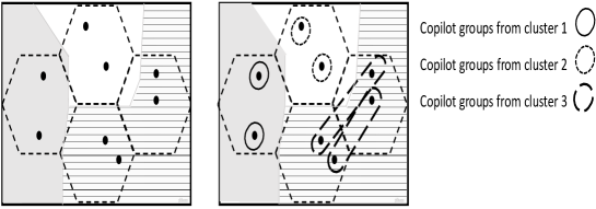
Figure 1: Example of the adaptive coherence-time based user scheduling procedure with $C=4,K=2,N_{g}=6,N_{c}=3$. Left: illustration of Step 2). Right: illustration of Step 3).

III-B Spectral efficiency with outdated CSI

We now investigate the achievable spectral efficiency when the aforementioned procedure is applied. For the sake of analytical traceability, we consider that all copilot groups contain exactly $C$ users. We, henceforth, refer to each user by its copilot group and serving BS indexes $g,l$. During uplink data transmission, the $j^{th}$ BS receives the following data signal at time slot $t$:

$$Y^{[j]}_{u}(t) =\sum_{l=1}^{C}\sum_{g=1}^{N_{g}}\sqrt{P_{u}}g^{[j]}_{gl}(t)S_{gl}+W_{u}(t),$$

where $P_{u}$ denotes the reverse link transmit power, $W_{u}(t)\sim CN(0,I_{M})$ is the additive noise and $S_{gl}$ denotes the uplink signal of the user from copilot group $g$ in cell $l$. In what follows we derive lower bounds on the achievable sum rate with a matched filter receiver when outdated CSI is used. At the reception, the $j^{th}$ BS applies a matched filter receiver based on the latest version of estimated CSI for the scheduled users. The resulting average achievable sum rate in the system is given in the following theorem. The proof can be found in Appendix A in [13].

Theorem 1.

The network serves $N_{g}$ copilot groups, $\tau$ of which are scheduled for uplink training. Using a matched filter receiver based on the latest available CSI estimates for each group, the average achievable sum rate $R_{u}$ in the uplink is lower bounded by:

$$R_{u}\geq\sum_{l=1}^{C}\sum_{g=1}^{N_{g}}\left(1-\frac{\tau}{T_{s}}\right)\text{log}\left(1+\frac{(M-1)\beta^{[l]^{2}}_{gl}\rho^{[l]^{2d_{g}}}_{gl}}{(M-1)\times I^{p}_{gl}+I^{n}_{gl}}\right),$$

where $d_{g},g=1...N_{g}$ represents the CSI delays of users using the same pilot sequence. $I^{p}_{gl}$ and $I^{n}_{gl}$ are given by:

$$I^{p}_{gl}=\sum_{c\neq l}^{C}\rho^{[l]^{2d_{g}}}_{gc}\beta^{[l]^{2}}_{gc},$$

$$I^{n}_{gl}=(\sum_{c=1}^{C}\sum_{k\neq g}\beta^{[l]}_{kc}+\sum_{c=1}^{C}(\beta^{[l]}_{gc}-\rho^{[l]^{2d_{g}}}_{gc}\frac{\beta^{[l]^{2}}_{gc}}{\frac{1}{P_{p}}+\sum_{b=1}^{C}\beta^{[l]}_{gb}})$$

$$+\frac{1}{P_{u}})\times(\frac{1}{P_{p}}+\sum_{b=1}^{C}\beta^{[l]}_{gb}).$$

Equation $(8)$ provides further insights into the evolution of the achievable sum rate as a function of the CSI time offset. The achievable sum rate for a given copilot user group decreases as the time offset increases since the correlation between the estimated CSI and the actual channel fades over time. In order to investigate the potential gain that the proposed approach can provide, we compare it with a reference model in which all of the $N_{g}$ copilot groups take part in the uplink training at each time slot, as in classical TDD protocols. This comparison is done in the next theorem where we consider the asymptotic regime (as $M$ grows large). The proof can be found in Appendix B in [13].

Theorem 2.

In the asymptotic regime, the proposed training approach enables to improve the achievable spectral efficiency of each user if the following condition is satisfied $\forall\;\lambda_{g},g=1,...,N_{g}$:

$$\left(\frac{\bar{\rho}^{[{min}]^{2}}_{g}}{\bar{\rho}^{[{max}]^{2}}_{{g}}}\right)^{d_{g}}\geq\frac{\left(1+\text{ SINR}^{[\infty]}_{g,l}\right)^{\frac{T_{s}-N_{g}}{T_{s}-\tau}}-1}{\text{ SINR}^{[\infty]}_{g,l}},$$

with

$$\text{ SINR}^{[\infty]}_{g,l}=\frac{\beta^{[l]^{2}}_{gl}}{\sum_{b\neq l}\beta^{[l]^{2}}_{gb}},$$

and $\bar{\rho}^{[{min}]}_{g}$ and $\bar{\rho}^{[{max}]}_{{g}}$ the minimum and maximum channel autocorrelation coefficients in group $g$, respectively.

Condition $(11)$ ensures that the achievable spectral efficiency of all users is improved when outdated CSI is used. We can see that the gain in spectral efficiency is maintained as long as the SINR degradation over time is compensated by the spared resources from uplink training. It also implies that the ratio between the maximum and minimum autocorrelation should be bounded. The bound becomes tighter as the allowed CSI delay increases. This condition is quite intuitive. It means that copilot users are required to experience comparable channel aging effects in order to be able to improve the achievable spectral efficiency using less uplink training. In order for Condition (11) to be satisfied we need users from the same copilot group to have equivalent coherence times and, consequently, they proceed to uplink training with the same periodicity. This is the reason why in Step $2)$ of the scheme proposed in Section III.A we group the mobile users according to channel autocorrelation coefficients. Next, we provide an efficient user scheduling method for uplink training. It exploits the autocorrelation based grouping in order to improve the achievable weighted sum rate. We consider that all copilot groups are active during data transmission. The network is required to select which groups will refresh their CSI by scheduling them for training.

IV Improving the achievable weighted sum rate

Assuming a constant coherence interval for all users results in a suboptimal resources exploitation since in practice, users experience heterogeneous Doppler frequencies. We showed, in Theorem $2$, that allowing the network to use outdated CSI estimates can actually improve the achievable spectral efficiency. In this section, we study the impact of the proposed adaptive training scheme on the achievable weighted sum rate. In this case, scheduling users for uplink training does not depend solely on the estimated CSI but also on the users traffic pattern. In order to take into consideration the QoS, we consider optimizing the weighted sum of rates. The weights enable to introduce fairness in the scheduling procedure [14]. We denote the weights associated with the users by $w_{gl},\;\forall g=1,...,N_{g},\;l=1,...,C$.

The aim here is to schedule copilot groups for uplink training in order to maximize the achievable weighted sum rate. As in previous sections we assume that all users are scheduled for data transmission and $\tau<N_{g}$ copilot groups are selected to update their CSI. Grouping users based on their autocorrelation coefficients simplifies the scheduling problem. Instead of deciding, at each time slot, to which user each pilot sequence is going to be allocated, decisions are made on predefined collections of copilot users. We define the vector $Y=(y_{1},\ldots,y_{N_{g}})$, with $y_{g},\forall g=1,...,N_{g}$ given by

$$y_{g}=\begin{cases}1&\mbox{if group $g$ is scheduled for training,}\\ 0&\mbox{otherwise. }\end{cases}$$ (13)

The copilot group scheduling problem when outdated CSI use is permitted, is formulated as follow

$$\underset{Y}{\text{max}} (1-\frac{\sum_{g=1}^{N_{g}}y_{g}}{T_{s}})\sum_{l=1}^{C}\sum_{g=1}^{N_{g}}w_{gl}R_{gl}(\vec{d},Y),$$ (14)

subject to $$\sum_{g=1}^{N_{g}}y_{g}\leq\tau,$$

where $R_{gl}(\vec{d},Y)$ is the lower bound on the achievable sum rate for the user in copilot group $g$ and cell $l$ (see Eq. (8)), and $\vec{d}$ is the delay vector. Here, $(14a)$ captures the fact that the number of scheduled users for uplink training in each cell, is at maximum equal to $\tau$. In the following theorem, we show that problem $(14)$ is equivalent to maximizing a submodular set function subject to a cardinality constraint. This formulation enables to apply a low complexity algorithm that solves the problem. The proof can be found in Appendix C in [13].

Theorem 3.

Problem $(14)$ is equivalent to maximizing a submodular set function with a cardinality constraint.

In order to solve problem $(14)$, we use the Submod-Max-Cardinality algorithm in Gupta et al. [15]. This algorithm starts by running the commonly used greedy approach, see Nemhauser et al. [16]. This provides a first candidate solution $S_{1}$. The approximation algorithm of Feige et al. [17] is then used on $S_{1}$ in order to obtain a second candidate solution $S_{2}$. The same steps are repeated on the remaining set of copilot groups that were not selected in $S_{1}$. The algorithm returns then the best found solution. When used to solve a non-monotone submodular function maximization subject to a cardinality constraint, Submod-Max-Cardinality yields a $(4+\alpha)$-approximation of the optimal solution [15]. The detailed algorithm can be found in Section IV [13]

V Numerical Results

In this section we provide some numerical results demonstrating the performance of the proposed training/copilot group scheduling scheme. Our training procedure is compared with a massive MIMO system operating according to the classical TDD protocol, considered as a reference model. We consider an hexagonal cell network with $C=7$ cells. Each cell has a $1.5\;\text{Km}$ radius. The mobile users are located uniformly at random in each cell and we assume that no user is closer than $r_{0}=10\;\text{m}$ to its serving BS. We consider heterogeneous movement speeds and directions. User speeds are randomly generated in the interval $\left[20\;\text{Km/h}\;,\;80\;\text{Km/h}\right]$. User movement direction, which is defined by the angle between the movement direction of the mobile device and the direction of the incident wave, is also randomly generated over the interval $\left[0\;,\;2\pi\right]$. We consider a path-loss exponent $\sigma=3.5$ and a relatively short coherence block of $T_{s}=200$ symbols is considered. We suppose a $200\;Mhz$ bandwidth [18]. The spectral efficiency is measured in bits/s/hz. The CSI delays for each copilot group $d_{g},g=1,...,N_{g}$ are selected randomly over the interval $[0,d_{max}]$.

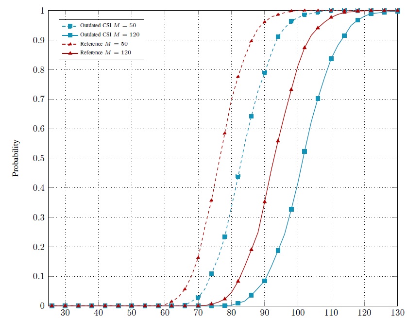
Figure 2: Comparison of the CDFs of spectral efficiency ($N_{g}=30,\;\tau=15,\;d_{max}=2$ )

In Figure 2, we illustrate a comparison of the CDFs of the achievable spectral efficiency between the reference model and the proposed outdated CSI based training scheme for different numbers of antennas at the BS. Figure 2 shows that, for $50$ receive antennas at the BS, the proposed training scheme achieves $5\%$-outage rate around $71\;\;\text{bit/s/hz}$. This performance represents a gain of $5\;\text{bit/s/hz}$ or, equivalently, $1000\;\text{Mbit/s}$ for a system bandwidth of $200\;Mhz$ [18], compared with the reference model that achieves $5\%$ outage rate around $66\;\;\text{bit/s/hz}$. For $120$ antennas at the BS, the gain in the $5\%$-outage rate when, outdated CSI is used, attains $1400\;\text{Mbit/s}$. In fact, while the proposed training scheme achieves $5\%$-outage rate around $87\;\;\text{bit/s/hz}$, the reference model achieves the same outage rate around $80\;\;\text{bit/s/hz}$. This gain comes from the spared resources during uplink training. In fact, using outdated CSI enables to increase the number of channel uses that are allocated to data transmission.

Figure 3: Spectral efficiency for varying values of $M$ ($N_{g}=30,\;\tau=15,\;d_{max}=2$)

In Figure 3, we illustrate the relation between the achievable spectral efficiency and the number of BS antennas. We compare the lower bound in Theorem $1$ with a simulated curve. Figure 3 shows that the derived is tight for a wide range of $M$. This figure also shows that, when compared with the reference model, the proposed training scheme increases the achievable spectral efficiency by $6.8\;\text{bit/s/hz}$ for $M=50$. This is equivalent to a rate gain of $1360\;\text{Mbit/s}$ for a system bandwidth of $200\;Mhz$ [18]. This gain attains $9.9\;\text{bit/s/hz}$ or, equivalently, $1980\;\text{Mbit/s}$ for $M=150$.

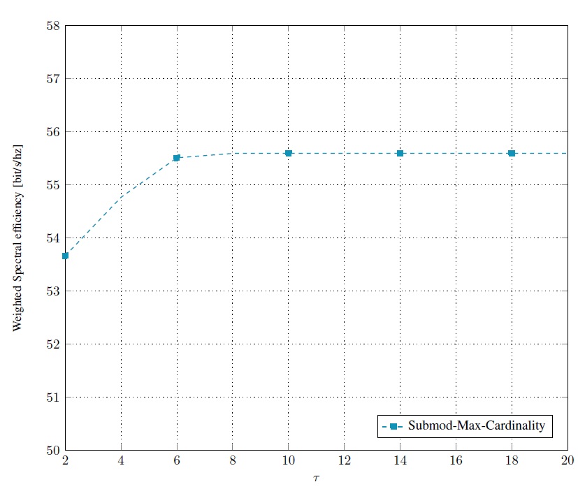
Figure 4: Weighted Spectral efficiency for varying value of $\tau$ ($N_{g}=20,\;M=100,\;d_{max}=3$ )

In Figure 4, we illustrate the performance of the proposed training/copilot group scheduling scheme. The weights $w_{gl},\;\forall g=1,...,N_{g},\;l=1,...,C$ are randomly generated in the interval $[0,1]$. Figure 4 shows that the optimal weighted sum rate saturate at $\tau=8$. This means that the optimal number of copilot groups scheduled for uplink training is $8$ in this setting. Consequently, scheduling more users for training will not result in a weighted sum rate gain. This actually concords with the suggestion that not all users who are active for data transmission are required to participate in uplink training. Consequently, an adaptive training scheme that takes into consideration CSI aging is justified.

VI Conclusion

In this paper, we studied the achievable sum rate in a massive MIMO system with a matched filter receiver taking into account the channel aging effect. We proposed a training scheme in which, we deliberately utilize outdated CSI estimates in order to optimize uplink training. The derived results show that, although outdated CSI degrades the achievable channel gain, we are able to achieve better spectral efficiency when training frequency is adapted to the channel’s autocorrelation. We show that, grouping the users in autocorrelation based clusters and optimizing their scheduling accordingly, provides a substantial increase in the achievable weighted sum rate. Future works will include investigating more sophisticated algorithms that enable to further leverage heterogeneous coherence times.

VII Appendix

VII-A Proof of Theorem 1

The network serves $N_{g}$ copilot groups, $\tau$ of which are scheduled for uplink training. At the reception, each BS uses a matched filter receiver that is based on the latest available CSI estimates. BS $l$ detects the signal of user $g$ in cell $l$ by applying the following filter

$$u_{gl}(t)=\frac{\hat{g}^{[l]}_{gl}(t-d_{g})}{\lVert\hat{g}^{[l]}_{gl}(t-d_{g})\rVert},t\geq d_{g},$$ (17)

where $\hat{g}^{[l]}_{gl}(t-d_{g})$ denotes the latest available CSI estimate for user $g$ in cell $l$. Consequently, the detected signal of user $g$ in cell $l$ is given by the following

$$u_{gl}^{\dagger}(t)\frac{Y^{[l]}_{u}(t)}{\sqrt{P_{u}}} =u_{gl}^{\dagger}(t)(\sum_{k=1}^{N_{g}}\sum_{c=1}^{C}g^{[l]}_{kc}(t)S_{kc}+\frac{W_{u}(t)}{\sqrt{P_{u}}})$$

$$=u_{gl}^{\dagger}(t)(g_{gl}^{[l]}(t)S_{gl}+\sum_{c\neq l}^{C}g_{gc}^{[l]}(t)S_{gc}+\sum_{k\neq g}^{N_{g}}\sum_{c=1}^{C}g_{kc}^{[l]}(t)S_{kc}+\frac{W_{u}(t)}{\sqrt{P_{u}}})$$

$$=u_{gl}^{\dagger}(t)((\rho^{[l]}_{gl})^{d_{g}}\hat{g}_{gl}^{[l]}(t-d_{g})S_{gl}+\sum_{c\neq l}^{C}(\rho^{[l]}_{gc})^{d_{g}}\hat{g}_{gc}^{[l]}(t-d_{g})S_{gc}+\sum_{c=1}^{C}(\rho^{[l]}_{gc})^{d_{g}}\tilde{g}_{gc}^{[l]}(t-d_{g})S_{gc}$$

$$+\sum_{c=1}^{C}\sum_{j=0}^{d_{g}-1}(\rho^{[l]}_{gc})^{j}\sqrt{\beta_{gc}^{[l]}}\varepsilon_{gc}^{[l]}(t-j)S_{gc}+\sum_{k\neq g}^{N_{g}}\sum_{c=1}^{C}g_{kc}^{[l]}(t)S_{kc}+\frac{W_{u}(t)}{\sqrt{P_{u}}})$$

$$=u_{il}^{\dagger}(t)(I_{1}(t)+I_{2}(t)+I_{3}(t)),$$

with

$$I_{1}(t) =(\rho^{[l]}_{gl})^{d_{g}}\hat{g}_{gl}^{[l]}(t-d_{g})S_{gl},$$

$$I_{2}(t) =\sum_{c\neq l}^{C}(\rho^{[l]}_{gc})^{d_{g}}\hat{g}_{gc}^{[l]}(t-d_{g})S_{gc},$$

$$I_{3}(t) =\sum_{c=1}^{C}(\rho^{[l]}_{gc})^{d_{g}}\tilde{g}_{gc}^{[l]}(t-d_{g})S_{gc}+\sum_{c=1}^{C}\sum_{j=0}^{d_{g}-1}(\rho^{[l]}_{gc})^{j}\sqrt{\beta_{gc}^{[l]}}\varepsilon_{gc}^{[l]}(t-j)S_{gc}+\sum_{k\neq g}^{N_{g}}\sum_{c=1}^{C}g_{kc}^{[l]}(t)S_{kc}+\frac{W_{u}(t)}{\sqrt{P_{u}}}$$

The third equality in Equation $(18)$ follows from the fact that $g_{ic}^{[l]}(t)=\sqrt{\beta_{ic}^{[l]}}h_{ic}^{[l]}(t)$, $h_{ic}^{[l]}(t)=\rho_{ic}^{[l]}h_{ic}^{[l]}(t-1)+\varepsilon_{ic}^{[l]}(t)$ for all $t$ and $g_{ic}^{[l]}(t)=\hat{g}_{ic}^{[l]}(t)+\tilde{g}_{ic}^{[l]}(t)$ for all $t$.

We note that $I_{1}(\cdot)$ refers to the useful signal, $I_{2}(\cdot)$ represents the impact of pilot contamination and $I_{3}(\cdot)$ regroups the impact of the white noise, channel estimation error, non correlated interference due to users with different pilot sequences and the impact of channel aging. The instant spectral efficiency attained by user $g$ in cell $l$ is:

$$R_{g,l}=\left(1-\frac{\tau}{T_{s}}\right)\log\left(1+\frac{|u_{gl}^{\dagger}(t)I_{1}(t)|^{2}}{|u_{gl}^{\dagger}(t)I_{2}(t)|^{2}+|u_{gl}^{\dagger}(t)I_{3}(t)|^{2}}\right).$$ (19)

We now define $\overline{R}_{g,l}$ to be the average achievable sum rate of user $g$ in cell $l$, namely,

$$\overline{R}_{g,l} =\mathbb{E}\left(\left(1-\frac{\tau}{T_{s}}\right)\log\left(1+\frac{|u_{gl}^{\dagger}(t)I_{1}(t)|^{2}}{|u_{gl}^{\dagger}(t)I_{2}(t)|^{2}+|u_{gl}^{\dagger}(t)I_{3}(t)|^{2}}\right)\right)$$ (20)

$$=\mathbb{E}\left(\mathbb{E}\left(\left(1-\frac{\tau}{T_{s}}\right)\log\left(1+\frac{|u_{gl}^{\dagger}(t)I_{1}(t)|^{2}}{|u_{gl}^{\dagger}(t)I_{2}(t)|^{2}+|u_{gl}^{\dagger}(t)I_{3}(t)|^{2}}\right)\bigg{|}\hat{g}_{gl}^{[l]}(t-d_{g})\right)\right),$$

the last equality follows from the law of total expectation. Let us define $\overline{R}_{g,l}^{0}$ such that

$$\overline{R}_{g,l}^{0}=\mathbb{E}\left(\left(1-\frac{\tau}{T_{s}}\right)\log\left(1+\frac{|u_{gl}^{\dagger}(t)I_{1}(t)|^{2}}{|u_{gl}^{\dagger}(t)I_{2}(t)|^{2}+|u_{gl}^{\dagger}(t)I_{3}(t)|^{2}}\right)\bigg{|}\hat{g}_{gl}^{[l]}(t-d_{g})\right),$$ (21)

therefore,

$$\overline{R}_{g,l}=\mathbb{E}(\overline{R}_{g,l}^{0}).$$ (22)

Based on the convexity of $\text{log}(1+\frac{1}{x+a})$, and Jensen’s inequality the following inequality can be obtained

$$\overline{R}^{0}_{g,l}\geq\left(1-\frac{\tau}{T_{s}}\right)\log\left(1+\frac{|u_{gl}^{\dagger}(t)(\rho_{gl}^{[l]})^{d_{g}}\hat{g}_{gl}^{[l]}(t-d_{g})|^{2}}{\mathbb{E}(|u_{gl}^{\dagger}(t)I_{2}(t)|^{2}|\hat{g}_{gl}^{[l]}(t-d_{g}))+\mathbb{E}(|u_{gl}^{\dagger}(t)I_{3}(t)|^{2}|\hat{g}_{gl}^{[l]}(t-d_{g}))}\right),$$ (23)

since

$$\mathbb{E}(|u_{gl}^{\dagger}(t)I_{1}(t)|^{2}|\hat{g}_{gl}^{[l]}(t-d_{g}))=|u_{gl}^{\dagger}(t)(\rho_{gl}^{[l]})^{d_{g}}\hat{g}_{gl}^{[l]}(t-d_{g})|^{2},$$ (24)

by the property $\mathbb{E}(f(Z)|Z)=f(Z)$ for a random variable $Z$. We now aim at computing $\mathbb{E}(|u_{gl}^{\dagger}(t)I_{j}(t)|^{2}|\hat{g}_{gl}^{[l]}(t-d_{g}))\hbox{ for }j=2,3.$ In order to do so, we are first going to obtain an alternative expression for $I_{2}(t)$, that is,

$$I_{2}(t) =\sum_{c\neq l}^{C}\hat{g}_{gc}^{[l]}(t-d_{g})S_{gc}=\hat{g}_{gl}^{[l]}(t-d_{g})\sum_{c\neq l}^{C}\frac{\beta_{gc}^{[l]}}{\beta_{gl}^{[l]}}S_{gc},$$ (25)

since $\hat{g}_{gc}^{[l]}(t-d_{g})=\hat{g}_{gl}^{[l]}(t-d_{g})\frac{\beta_{gc}^{[l]}}{\beta_{gl}^{[l]}}$. Therefore, $I_{2}(t)$ and $\hat{g}_{gl}^{[l]}(t-d_{g})$ are correlated. Consequently, we obtain

$${\mathbb{E}}\left[|u_{gl}^{\dagger}(t)I_{2}(t)|^{2}|\hat{g}_{gl}^{[l]}(t-d_{g})\right]=\left|u_{gl}^{\dagger}(t)\hat{g}^{[l]}_{gl}(t-d_{g})\right|^{2}\sum_{c\neq l}^{C}(\rho^{[l]}_{gc})^{2d_{g}}\frac{\beta^{[l]^{2}}_{gc}}{\beta^{[l]^{2}}_{gl}}.$$ (26)

We will now compute $\mathbb{E}(|u_{gl}^{\dagger}(t)I_{3}(t)|^{2}|\hat{g}_{gl}^{[l]}(t-d_{g}))$. First note that, $I_{3}(t)$ is independent of $\hat{g}_{gl}^{[l]}(t-d_{g})$ and since $u_{gl}^{\dagger}(t)$ has unit norm, we have that $\mathbb{E}(|u_{gl}^{\dagger}(t)I_{3}(t)|^{2}|\hat{g}_{gl}^{[l]}(t-d_{g}))=\mathbb{E}(|I_{3}(t)|^{2})$, therefore we obtain

$$\mathbb{E}(|I_{3}(t)|^{2}) =\mathbb{E}\bigg{(}|\sum_{c=1}^{C}(\rho_{gc}^{[l]})^{d_{g}}\tilde{g}_{gc}^{[l]}(t-d_{g})S_{gc}+\sum_{c=1}^{C}\sum_{j=0}^{d_{g}-1}\sqrt{\beta_{gc}^{[l]}}(\rho_{gc}^{[l]})^{j}\varepsilon_{gc}^{[l]}(t-j)S_{gc}$$

$$+\sum_{k\neq g}^{N_{g}}\sum_{c=1}^{C}g_{kc}^{[l]}(t)S_{kc}+\frac{W_{u}(t)}{\sqrt{P_{u}}}|^{2}\bigg{)}$$

$$=\mathbb{E}\bigg{(}\sum_{c=1}^{C}|(\rho_{gc}^{[l]})^{d_{g}}\tilde{g}_{gc}^{[l]}(t-d_{g})|^{2}+\sum_{c=1}^{C}\sum_{j=0}^{d_{g}-1}|\sqrt{\beta_{gc}^{[l]}}(\rho_{gc}^{[l]})^{j}\varepsilon_{gc}^{[l]}(t-j)|^{2}$$

$$+\sum_{k\neq g}^{N_{g}}\sum_{c=1}^{C}|g_{kc}^{[l]}(t)|^{2}+|\frac{W_{u}(t)}{\sqrt{P_{u}}}|^{2}\bigg{)},$$

where the last equality follows from noting the following four properties; (i) $S_{kc}\cdot S_{ic^{\prime}}=0$ for all $k\neq i$ and all $c,c^{\prime}\in\{0,\ldots,C\}$, (ii) $\mathbb{E}(ZW_{u}(t))=\mathbb{E}(Z)\mathbb{E}(W_{u}(t))=0$ for all random variables $Z$ that are independent of $W_{u}(t)$ (zero mean complex Gaussian noise), (iii) similar to the previous property, $\mathbb{E}(Z\varepsilon_{ic}^{[l]}(t))=\mathbb{E}(Z)\mathbb{E}(\varepsilon_{ic}^{[l]}(t))=0$ for all $Z$ independent of $\varepsilon_{ic}^{[l]}(t)$ (zero mean complex white Gaussian noise) and finally (iv) $g_{kc}^{[l]}$ and $\tilde{g}_{k^{\prime}c^{\prime}}^{[l]}$ are independent for all $(k,c)\neq(k^{\prime},c^{\prime})$. We now compute the four terms in Equation $(27)$. The last term, i.e.,

$$\mathbb{E}(|W_{u}(t)/\sqrt{P_{u}}|^{2})=\frac{1}{P_{u}}.$$ (28)

Next we compute the second term in Equation $(27)$, namely,

$$\mathbb{E}(\sum_{c=1}^{C}|(\rho_{gc}^{[l]})^{d_{g}}\tilde{g}_{gc}^{[l]}(t-d_{g})|^{2})=\sum_{c=1}^{C}(\rho_{gc}^{[l]})^{2d_{g}}\left(\beta_{gc}^{[l]}-\frac{(\beta_{gc}^{[l]})^{2}}{\frac{1}{P_{p}}+\sum_{b=1}^{C}\beta_{gb}^{[l]}}\right).$$ (29)

the latter is satisfied due to the fact that the variance of $\tilde{g}_{gc}^{[l]}(t-d_{g})$ being given by $\beta_{gc}^{[l]}-\frac{(\beta_{gc}^{[l]})^{2}}{\frac{1}{P_{p}}+\sum_{b=1}^{C}\beta_{gb}^{[l]}}$ for all $g$ and $c$.

We now compute the third term in Equation $(27)$, that is,

$$\mathbb{E}\left(\sum_{c=1}^{C}\sum_{j=0}^{d_{g}-1}|\sqrt{\beta_{gc}^{[l]}}(\rho_{gc}^{[l]})^{j}\varepsilon_{gc}^{[l]}(t-j)|^{2}\right) =\sum_{c=1}^{C}\sum_{j=0}^{d_{g}-1}\beta_{gc}^{[l]}(\rho_{gc}^{[l]})^{2j}(1-(\rho_{gc}^{[l]})^{2})$$

$$=\sum_{c=1}^{C}\beta_{gc}^{[l]}\frac{1-(\rho_{gc}^{[l]})^{2d_{g}}}{1-(\rho_{gc}^{[l]})^{2}}(1-(\rho_{gc}^{[l]})^{2})$$

$$=\sum_{c=1}^{C}\beta_{gc}^{[l]}({1-(\rho_{gc}^{[l]})^{2d_{g}}}),$$

for the second equality we have used the expression of finite geometric sums since $(\rho_{gc}^{[l]})^{2}<1$ for all $g$ and $c$. We are left with the first term in Equation $(27)$, that is,

$$\sum_{k\neq g}^{N_{g}}\sum_{c=1}^{C}\mathbb{E}(|g_{kc}^{[l]}(t)|^{2})=\sum_{k\neq g}^{N_{g}}\sum_{c=1}^{C}\mathbb{E}(|\sqrt{\beta_{kc}^{[l]}}h_{kc}^{[l]}(t)|^{2})=\sum_{k\neq g}^{N_{g}}\sum_{c=1}^{C}\beta_{kc}^{[l]},$$

Combining all four terms, that is, Equations $(28)$, $(29)$, $(30)$ and $(31)$, we obtain

$${\mathbb{E}}\left[|u_{gl}^{\dagger}(t)I_{3}(t)|^{2}\right] =\sum_{k\neq g}^{N_{g}}\sum_{c=1}^{C}\beta_{kn}^{[l]}+\sum_{c=1}^{C}\beta_{gc}^{[l]}({1-(\rho_{gc}^{[l]})^{2d_{g}}})+\sum_{c=1}^{C}(\rho_{gc}^{[l]})^{2d_{g}}\left(\beta_{gc}^{[l]}-\frac{(\beta_{gc}^{[l]})^{2}}{\frac{1}{P_{p}}+\sum_{b=1}^{C}\beta_{gb}^{[l]}}\right)$$

$$=\sum_{k\neq g}^{N_{g}}\sum_{c=1}^{C}\beta_{kc}^{[l]}+\sum_{c=1}^{C}(\beta^{[l]}_{gc}-\rho^{[l]^{2d_{g}}}_{gc}\frac{\beta^{[l]^{2}}_{gc}}{\frac{1}{P_{p}}+\sum_{b=1}^{C}\beta^{[l]}_{gb}})+\frac{1}{P_{u}}.$$

Substituting the results in Equations $(24)$, $(26)$ and $(32)$ in Equation $(21)$, we obtain

$$\overline{R}_{g,l}^{0} \geq\left(1-\frac{\tau}{T_{s}}\right)\log\left(1+\frac{(\rho_{gl}^{[l]})^{2d_{g}}|u_{gl}^{\dagger}(t)\hat{g}_{gl}^{[l]}(t-d_{g})|^{2}}{F}\right),$$ (33)

with

$$F= |u_{gl}^{\dagger}(t)\hat{g}_{gl}^{[l]}(t-d_{g})|^{2}\sum_{c\neq l}^{C}(\rho^{[l]}_{gc})^{2d_{g}}\frac{\beta^{[l]^{2}}_{gc}}{\beta^{[l]^{2}}_{gl}}+\sum_{k\neq g}^{N_{g}}\sum_{c=1}^{C}\beta_{kc}^{[l]}+\sum_{c=1}^{C}(\beta^{[l]}_{gc}-\rho^{[l]^{2d_{g}}}_{gc}\frac{\beta^{[l]^{2}}_{gc}}{\frac{1}{P_{p}}+\sum_{b=1}^{C}\beta^{[l]}_{gb}})+\frac{1}{P_{u}}.$$

From Equation $(20)$ and Equation $(33)$ we obtain

$$\overline{R}_{g,l}=\mathbb{E}(\overline{R}_{g,l}^{0}) =\mathbb{E}\left(\left(1-\frac{\tau}{T_{s}}\right)\log\left(1+\frac{(\rho_{il}^{[l]})^{2d_{g}}|u_{il}^{\dagger}(t)\hat{g}_{il}^{[l]}(t-d_{g})|^{2}}{F}\right)\right)$$

$$=\mathbb{E}\left(\left(1-\frac{\tau}{T_{s}}\right)\log\left(1+\frac{(\rho_{gl}^{[l]})^{2d_{g}}}{G}\right)\right),$$

where

$$G= \frac{F}{|u_{gl}^{\dagger}(t)\hat{g}_{gl}^{[l]}(t-d_{g})|^{2}}.$$

In order to compute the final expression of the bound on the average rate, it now suffices to compute the explicit expression of the right hand side (RHS) of Equation $(35)$. In order to do so, we apply Jensen’s inequality to the RHS in Eq. $(35)$, that is,

$$\overline{R}_{g,l} \geq\left(1-\frac{\tau}{T_{s}}\right)\log\left(1+\frac{(\rho_{g,l}^{[l]})^{2d_{g}}}{\mathbb{E}(G)}\right),$$ (36)

with

$$\mathbb{E}(G)= \sum_{c\neq l}^{C}(\rho^{[l]}_{gc})^{2d_{g}}\frac{\beta^{[l]^{2}}_{gc}}{\beta^{[l]^{2}}_{gl}}+\mathbb{E}\left(\frac{1}{|u_{gl}^{\dagger}(t)\hat{g}_{gl}^{[l]}(t-d_{g})|^{2}}\right)$$ (37)

$$\cdot\left(\sum_{k\neq g}^{N_{g}}\sum_{c=1}^{C}\beta_{kc}^{[l]}+\sum_{c=1}^{C}(\beta^{[l]}_{gc}-\rho^{[l]^{2d_{g}}}_{gc}\frac{\beta^{[l]^{2}}_{gc}}{\frac{1}{P_{p}}+\sum_{b=1}^{C}\beta^{[l]}_{gb}})+\frac{1}{P_{u}}\right).$$

Note that $\left|u_{gl}^{\dagger}(t)\hat{g}^{[l]}_{gl}(t-d_{g})\right|^{2}$ has a Gamma distribution with parameters $(M,\frac{\beta^{[l]^{2}}_{gl}}{\frac{1}{P_{p}}+\sum_{b=1}^{C}\beta^{[l]}_{gb}})$. Consequently, the mean value of $\frac{1}{\left|u_{gl}^{\dagger}(t)\hat{g}^{[l]}_{gl}(t-d_{g})\right|^{2}}$ (that has an inverse Gamma distribution) is equal to $\frac{1}{(M-1)\times\frac{\beta^{[l]^{2}}_{gl}}{\frac{1}{P_{p}}+\sum_{b=1}^{C}\beta^{[l]}_{gb}}}$. Combining this together with the results in Equations $(37)$ and $(35)$ we obtain the desired lower bound on the average achievable spectral efficiency of user $g,l$, that is,

$$\overline{R}_{g,l} \geq\left(1-\frac{\tau}{T_{s}}\right)\text{log}\left(1+\frac{(M-1)(\beta^{[l]}_{gl})^{2}(\rho^{[l]}_{gl})^{2d_{g}}}{(M-1)I^{p}_{gl}+I^{n}_{gl}}\right),$$ (38)

where $I^{p}_{gl}$ and $I^{n}_{gl}$ are given by

$$I^{p}_{gl}=\sum_{c\neq l}^{C}(\rho^{[l]}_{gc})^{2d_{g}}(\beta^{[l]}_{gc})^{2},\hbox{ and }$$

$$I^{n}_{gl}=(\frac{1}{P_{p}}+\sum_{b=1}^{C}\beta^{[l]}_{gb})\cdot\left(\sum_{k\neq g}^{N_{g}}\sum_{c=1}^{C}\beta_{kc}^{[l]}+\sum_{c=1}^{C}(\beta^{[l]}_{gc}-\rho^{[l]^{2d_{g}}}_{gc}\frac{\beta^{[l]^{2}}_{gc}}{\frac{1}{P_{p}}+\sum_{b=1}^{C}\beta^{[l]}_{gb}})+\frac{1}{P_{u}}\right).$$

Summing the achievable spectral efficiency of all grouped users concludes the proof.

VII-B Proof of Theorem 2

In order to prove theorem 2, we consider the assymptotic regime where the number of BS antennas $M$ grows very large. In this case the lower bound on achievable spectral efficiency of each user $g,l$ converges to the following limit:

$$\left(1-\frac{\tau}{T_{s}}\right)\text{log}\left(1+\frac{(M-1)\beta^{[l]^{2}}_{gl}\rho^{[l]^{2d_{g}}}_{gl}}{(M-1)\times I^{p}_{gl}+I^{n}_{gl}}\right)\longrightarrow\left(1-\frac{\tau}{T_{s}}\right)\text{log}\left(1+\frac{\beta^{[l]^{2}}_{gl}\rho^{[l]^{2d_{g}}}_{gl}}{\sum_{b\neq l}^{C}\rho^{[l]^{2d_{g}}}_{gb}\beta^{[l]^{2}}_{gb}}\right).$$

The proposed framework is compared with a reference massive MIMO system where, all scheduled users are required to perform uplink training. In the asymptotic regime, the lower bound on the achievable spectral efficiency of each user $g,l$ in the reference system converges to the following limit:

$$\left(1-\frac{N_{g}}{T_{s}}\right)\text{log}\left(1+\frac{\beta^{[l]^{2}}_{gl}}{\sum_{b\neq l}^{C}\beta^{[l]^{2}}_{gb}}\right).$$ (40)

The aim here, is to improve the achievable spectral efficiency of each scheduled users. Consequently, the spectral efficiency of each user in the two considered systems should verify, $\;\forall\;g=1...N_{g},l=1...C$:

$$\left(1-\frac{\tau}{T_{s}}\right)\text{log}\left(1+\frac{\beta^{[l]^{2}}_{gl}\rho^{[l]^{2d_{g}}}_{gl}}{\sum_{b\neq l}^{C}\rho^{[l]^{2d_{g}}}_{gb}\beta^{[l]^{2}}_{gb}}\right)\geq\left(1-\frac{N_{g}}{T_{s}}\right)\text{log}\left(1+\frac{\beta^{[l]^{2}}_{gl}}{\sum_{b\neq l}^{C}\beta^{[l]^{2}}_{gb}}\right).$$

$(27)$ is equivalent to the following condition:

$$\frac{\beta^{[l]^{2}}_{gl}\rho^{[l]^{2d_{g}}}_{gl}}{\sum_{b\neq l}^{C}\rho^{[l]^{2d_{g}}}_{gb}\beta^{[l]^{2}}_{gb}}\geq\left(1+\frac{\beta^{[l]^{2}}_{gl}}{\sum_{b\neq l}^{C}\beta^{[l]^{2}}_{gb}}\right)^{\frac{T_{s}-N_{g}}{T_{s}-\tau}}-1.$$

We consider the extreme case where $\rho^{2}_{gl}=\bar{\rho}^{[{min}]^{2}}_{g}$ and $\forall b\neq l,\rho^{2}_{gb}=\bar{\rho}^{[{max}]^{2}}_{{g}}$. Here $\bar{\rho}^{[{min}]}_{g}$ and $\bar{\rho}^{[{max}]}_{{g}}$ denote respectively the minimum and maximum channel autocorrelation coefficients in group $g$. This means that we assume the worst case scenario for each user where, its coherence time is always lower than its fellow copilot users. Finally, by considering $SINR^{[\infty]}_{g,l}=\frac{\beta^{[l]^{2}}_{gl}}{\sum_{b\neq l}^{C}\beta^{[l]^{2}}_{gb}}$, we obtain $(11)$ which finishes the proof.

VII-C Proof of Theorem 3

In order to prove theorem $3$, we start by demonstrating that the objective function $f$ in $(14)$, is submodular. We consider two copilot groups allocations, $X\;\text{and}\;Z$ such that $X\subseteq Z$. We define the following ground set $G=\left\{x^{[g]},g=1...N_{g}\right\}$, where $x^{[g]},g=1...N_{g}$ is an abstract element denoting the scheduling of copilot group $g$ for uplink training. We need to prove that the marginal value of scheduling a new copilot group $x^{[n]}$ in $X$ and $Z$ verifies:

$$f\left(X\cup\left\{x^{[n]}\right\}\right)-f\left(X\right)\geq f\left(Z\cup\left\{x^{[n]}\right\}\right)-f\left(Z\right).$$

We start by computing the marginal values of adding an element $x^{[n]}$ to $X$ and $Z$ which are, respectively, given by:

$$f\left(X\cup\left\{x^{[n]}\right\}\right)-f\left(X\right)=\left(\frac{\lvert X\rvert}{T_{s}}-\frac{\lvert X\rvert+1}{T_{s}}\right)\{\sum_{l=1}^{C}\sum_{x^{[i]}\in X}w_{il}\text{log}\left(1+\frac{(M-1)\beta^{[l]^{2}}_{il}}{(M-1)\times I^{p}_{il}+I^{n}_{il}}\right)$$

$$+\sum_{x^{[i]}\in G\backslash[X\cup x^{[n]}]}w_{il}\text{log}\left(1+\frac{(M-1)\beta^{[l]^{2}}_{il}\rho^{[l]^{2d_{i}}}_{il}}{(M-1)\times I^{p}_{il}+I^{n}_{il}}\right)\}+(1-\frac{\lvert X\rvert+1}{T_{s}})w_{nl}\text{log}\left(1+\frac{(M-1)\beta^{[l]^{2}}_{nl}}{(M-1)\times I^{p}_{nl}+I^{n}_{nl}}\right)$$

$$-(1-\frac{\lvert X\rvert}{T_{s}})w_{nl}\text{log}\left(1+\frac{(M-1)\beta^{[l]^{2}}_{nl}\rho^{[l]^{2d_{n}}}_{nl}}{(M-1)\times I^{p}_{nl}+I^{n}_{nl}}\right),$$

and,

$$f\left(Z\cup\left\{x^{[n]}\right\}\right)-f\left(Z\right)=\left(\frac{\lvert Z\rvert}{T_{s}}-\frac{\lvert Z\rvert+1}{T_{s}}\right)\{\sum_{l=1}^{C}\sum_{x^{[i]}\in Z}w_{il}\text{log}\left(1+\frac{(M-1)\beta^{[l]^{2}}_{il}}{(M-1)\times I^{p}_{il}+I^{n}_{il}}\right)$$

$$+\sum_{x^{[i]}\in G\backslash[Z\cup x^{[n]}]}w_{il}\text{log}\left(1+\frac{(M-1)\beta^{[l]^{2}}_{il}\rho^{[l]^{2d_{i}}}_{il}}{(M-1)\times I^{p}_{il}+I^{n}_{il}}\right)\}+(1-\frac{\lvert Z\rvert+1}{T_{s}})w_{nl}\text{log}\left(1+\frac{(M-1)\beta^{[l]^{2}}_{nl}}{(M-1)\times I^{p}_{nl}+I^{n}_{nl}}\right)$$

$$-(1-\frac{\lvert Z\rvert}{T_{s}})w_{nl}\text{log}\left(1+\frac{(M-1)\beta^{[l]^{2}}_{nl}\rho^{[l]^{2d_{n}}}_{nl}}{(M-1)\times I^{p}_{nl}+I^{n}_{nl}}\right).$$

The difference between the two marginal values is given by:

$$f\left(X\cup\left\{x^{[n]}\right\}\right)-f\left(X\right)-(f\left(Z\cup\left\{x^{[n]}\right\}\right)-f\left(Z\right))=$$

$$[\frac{\lvert Z\rvert-\lvert X\rvert}{T_{s}}]w_{nl}\text{log}\left(1+\frac{(M-1)\beta^{[l]^{2}}_{nl}}{(M-1)\times I^{p}_{nl}+I^{n}_{nl}}\right)+[\frac{\lvert X\rvert-\lvert Z\rvert}{T_{s}}]w_{nl}\text{log}\left(1+\frac{(M-1)\beta^{[l]^{2}}_{nl}\rho^{[l]^{2d_{n}}}_{nl}}{(M-1)\times I^{p}_{nl}+I^{n}_{nl}}\right)$$

$$+\sum_{l=1}^{C}\sum_{x^{[i]}\in Z\backslash X}[\frac{w_{il}}{T_{s}}]\left(\text{log}\left(1+\frac{(M-1)\beta^{[l]^{2}}_{il}}{(M-1)\times I^{p}_{il}+I^{n}_{il}}\right)-\text{log}\left(1+\frac{(M-1)\beta^{[l]^{2}}_{il}\rho^{[l]^{2d_{i}}}_{il}}{(M-1)\times I^{p}_{il}+I^{n}_{il}}\right)\right).$$

The difference in marginal values is positive. Consequently, the objective function $f$ is submodular. In addition, it is clear that $(14a)$ is a cardinality constraint. Problem $(14)$ is then equivalent to maximizing a submodular function with a cardinality constraint.

References

• [1] T. L. Marzetta, Noncooperative cellular wireless with unlimited numbers of base station antennas, IEEE Trans. Wireless. Commun., vol. 9, no. 11, pp. 3590-3600, Nov. 2010.
• [2] Alexei Ashikhmin, Thomas L. Marzetta and Liangbin LiInterference Reduction in Multi-Cell Massive MIMO Systems I: Large-Scale Fading Precoding and Decoding, November 2014.
• [3] L. Thiele, M. Olbrich, M. Kurras, and B. Matthiesen, Channel aging effects in CoMP transmission: Gains from linear channel prediction, in Proc. Asilomar Conf. Signals Syst. Comput., Nov. 2011, pp. 1924-1928.
• [4] K. Truong and R. Heath, Effects of channel aging in massive MIMO systems, J. Commun. Netw., vol. 15, no. 4, pp. 338-351, Sep. 2013.
• [5] A. K. Papazafeiropoulos and T. Ratnarajah,Linear precoding for downlink massive MIMO with delayed CSIT and channel prediction, in Proc. IEEE Wireless Commun. Netw. Conf. (WCNC), Apr. 2014, pp. 809-914.
• [6] A. K. Papazafeiropoulos and T. Ratnarajah, Uplink performance of massive MIMO subject to delayed CSIT and anticipated channel prediction, in Proc. IEEE Int. Conf. Acoust. Speech Signal Process. (ICASSP), May 2014, pp. 3162-3165.
• [7] C. Kong, C. Zhong, A. K. Papazafeiropoulos, M. Matthaiou, and Z. Zhang, Sum-rate and power scaling of massive MIMO systems with channel aging, IEEE Trans. Commun., vol. 63, no. 12, pp. 4879-4893, Dec. 2015.
• [8] Thang X. Vu, Trinh Anh Vu, Symeon Chatzinotas and Bjorn Ottersten, Spectral-Efficient Model for Multiuser Massive MIMO: Exploiting User Velocity, IEEE ICC’17, Mai 2017
• [9] J. Cai, W. Song, and Z. Li, Doppler spread estimation for mobile OFDM systems in rayleigh fading channel, IEEE Trans. Consumer Electron., vol. 49, pp. 973.977, Nov. 2003.
• [10] W. C. Jakes, Ed., Microwave Mobile Communications. New York: Wiley, 1974.
• [11] S. Sesia, I. Toufik, and M. Baker, Eds., LTE: The UMTS Long Term Evolution. John Wiley and Sons, 2009.
• [12] T. Y. Young and T. W. Calvert, Classification, estimation and pattern recognition, American Elsevier Publishing Company, 1974.
• [13] S. Hajri and M. Assaad, M. Larrañaga, Enhancing massive MIMO: A new approach for Uplink training based on heterogeneous coherence times, http://www.l2s.centralesupelec.fr/perso/salah.hajri/publications
• [14] L. Tassiulas and A. Ephremides, Stability properties of constrained queueing systems and scheduling policies for maximum throughput in multihop radio networks, IEEE Trans. Automat. Contr., vol. 4, pp. 1936-1948, December 1992.
• [15] A. Gupta, A. Roth, G. Schoenebeck and K. Talwar. Constra ined non-monotone submodular maximiza- tion: Offline and secretary algorithms. Proc. of WINE , 2010. A more detailed version available at http://arxiv.org/abs/1003.1517v2.
• [16] G. L. Nemhauser, L. A. Wolsey, and M. L. Fisher, An analysis of approximations for maximizing submodular set functions i, Mathematical Programming, 14:265-294, 1978.
• [17] U. Feige, V. Mirrokni, and J. Vondrak. Maximizing non-monotone submodular functions. In Proceedings of 48th Annual IEEE Symposium on Foundations of Computer Science (FOCS) , 2007.
• [18] Geoff Varrall, 5G Spectrum and Standards, Artech House, 31 mai 2016