A Scalable Semidefinite Relaxation Approach to Grid Scheduling

Abstract.

Determination of the most economic strategies for supply and transmission of electricity is a daunting computational challenge. Due to theoretical barriers, so-called NP-hardness, the amount of effort to optimize the schedule of generating units and route of power, can grow exponentially with the number of decision variables. Practical approaches to this problem involve legacy approximations and ad-hoc heuristics that may undermine the efficiency and reliability of power system operations, that are ever growing in scale and complexity. Therefore, the development of powerful optimization methods for detailed power system scheduling is critical to the realization of smart grids and has received significant attention recently. In this paper, we propose for the first time a computational method, which is capable of solving large-scale power system scheduling problems with thousands of generating units, while accurately incorporating the nonlinear equations that govern the flow of electricity on the grid. The utilization of this accurate nonlinear model, as opposed to its linear approximations, results in a more efficient and transparent market design, as well as improvements in the reliability of power system operations. We design a polynomial-time solvable third-order semidefinite programming (TSDP) relaxation, with the aim of finding a near globally optimal solution for the original NP-hard problem. The proposed method is demonstrated on the largest available benchmark instances from real-world European grid data, for which provably optimal or near-optimal solutions are obtained.

July 2017

 
BCOL RESEARCH REPORT 17.03
Industrial Engineering & Operations Research
University of California, Berkeley, CA 94720–1777

The development of systematic algorithms for optimal allocation and scheduling of resources can be traced back to Nobel Laureate Wassily Leontief’s seminal work on input-output analysis [1], and the development of simplex algorithm by George Dantzig [2], which was driven by the United States military planning problems during World War II. Ever since, various application domains have relied heavily on optimization theory as a tool for design, planning, and decision-making.

An economically significant application is the operation of power grids, with the aim of efficient and secure supply of electricity. Grid operations are currently planned with legacy frameworks that are far from producing near-optimal solutions at the scale and detail required by the next-generation grids. In the past decade, various potential approaches have been identified for enhancements in grid operation through more accurate models for the flow of power, control of network topology, and taking uncertainties of demand and renewable generation into consideration. The realization of the aforementioned directions is expected to offer considerable improvements in the efficiency and reliability of the power grids [3]. However, due to the ever-growing size and scope of grids, the scalability of algorithms for solving detailed and accurate models remains as the primary bottleneck [4, 5, 6].

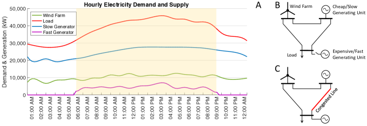
Figure 1. Day-ahead scheduling of a notional power system, with three vertices and two generating units. (A) The optimal operational strategy based on the available forecast of the demand and wind generation. The shaded period represents peak hours. (B) Off-peak configuration of the network, during which the expensive generator is not committed. (C) Peak configuration, during which the expensive generator contributes to accommodate transmission limits.

Building an optimal day-ahead plan for the operation of a nationwide grid is a daunting challenge, in part, due to the presence of thousands of generating units, whose on/off status need to be determined. Algorithms for finding the most economic plan with binary on/off decisions give rise to massive search trees. Another challenge is posed by the nonlinearity of the physical laws describing the flow of electricity.

This paper presents the first computational method that is capable of solving day-ahead power system scheduling problems of realistic size, that are built upon accurate physical models. More specifically, the proposed method accomplishes the integrated optimization of two fundamental problems, faced by system operators and utilities on a daily basis:

1. Unit Commitment (UC): The problem of scheduling generating units throughout a planning horizon, based on demand forecasts and technological constraints.

2. Optimal Power Flow (OPF): The problem of determining an operating point for the network that delivers power from suppliers to consumers as economically as possible, subject to physical constraints.

Advanced algorithms for UC and OPF can contribute to the efficiency and transparency of power markets by improving operational decisions and pricing mechanisms [7, 8]. Figure 1, exemplifies the optimal unit commitment plan for operating a notional power grid for the day-ahead, based on the available forecast of the demand and renewable generation. A cheap/slow unit provides the base generation for the entire planning horizon, while an expensive/fast generating unit is committed during the peak hours to avoid the violation of transmission limits.

The contributions of this paper are twofold. First the unit commitment problem is convexified via a family of linear and third-order semidefinite programming (TSDP) constraints. This convex relaxation achieves near-globally optimal solutions for UC problems with nearly $100,000$ binary variables. Second, a family of TSDP constraints are introduced to relax the power flow equations. The combination results in a tractable method for solving coupled UC-OPF optimization problems. The proposed method offers unprecedented scalability and improves upon the existing literature, in terms of the practical feasibility and efficiency of solutions, by allowing the joint optimization of commitment and power flow decisions based on an accurate nonlinear model for power grids.

0.1. Semidefinite Programming Relaxation

Since a wide range of physical phenomena and dynamical systems can be modeled by polynomial functions, polynomial optimization have received significant research interest. Our methodology is aligned with a popular framework for the study of polynomial optimization, that involves convex hull characterization of algebraic varieties through hierarchies of semidefinite programs (SDPs) [9, 10]. Performance guarantees and extensions of SDP hierarchies have since been investigated by several papers [11, 12, 13, 14], as well as their applications in various areas such as, quantum information theory [15, 16], compressed sensing [17, 18], graph theory [19, 20], statistics [21], operation of infrastructure networks [22, 23], and other branches of optimization theory [24]. The primary challenge for the application of SDP hierarchies beyond small-scale instances is the rapid growth of dimension, which necessitates a detailed study of sparsity and structural patterns to boost the efficiency [25, 26, 27, 28, 29].

Table 1. The performance of the TSDP relaxation algorithm for 24-hour horizon scheduling of benchmark systems with hourly epochs using the linear DC and nonlinear AC models.

		Linear DC Model					Nonlinear AC Model
Test Case​​	Number	Ratio of TSDP	TSDP	TSDP	CPLEX	CPLEX	Ratio of TSDP	TSDP	TSDP
	of Units	Inexact Binaries	Gap	Time	Gap	Time	Inexact Binaries	Gap	Time
IEEE 118​​	$54$	$0~{}/~{}1,296$	$0\%$	$3\mathrm{s}$	$0\%$	$28\mathrm{s}$	$0~{}/~{}1,296$	$0.01\%$	$11\mathrm{s}$
IEEE 300​​	$69$	$0~{}/~{}1,656$	$0\%$	$3\mathrm{s}$	$0\%$	$67\mathrm{s}$	$0~{}/~{}1,656$	$0.34\%$	$41\mathrm{s}$
PEGASE 1354​​	$193$	$28.4~{}/~{}4,632$	$0.09\%$	$18\mathrm{s}$	$8.57\%$	$10,800\mathrm{s}^{\dagger}$	$26.0~{}/~{}4,632$	$1.24\%$	$486\mathrm{s}$
PEGASE 2869​​	$392$	$24.5~{}/~{}9,408$	$0.01\%$	$35\mathrm{s}$	$-$	$10,800\mathrm{s}^{\dagger}$	$33.8~{}/~{}9,408$	$0.42\%$	$2,175\mathrm{s}$
PEGASE 9241​​	$1,153$	$75.4~{}/~{}27,672$	$0.05\%$	$137\mathrm{s}$	$-$	$10,800\mathrm{s}^{\dagger}$	$226.5~{}/~{}27,672$	$2.73\%$	$56,351\mathrm{s}$
PEGASE 13659​​	$4,077$	$29.5~{}/~{}97,848$	$0.22\%$	$266\mathrm{s}$	$-$	$10,800\mathrm{s}^{\dagger}$	$995.3~{}/~{}97,848$	$1.21\%$	$116,064\mathrm{s}$
$~{}^{\dagger}$ Solver is terminated after $3$ hours.

0.2. Review of Unit Commitment

Economic scheduling of power generation units has been extensively investigated since the early 1960s, to handle predictable demand variations throughout the day-ahead. Extensions of the problem have later been studied to capture practical limits of network and security requirements, among other considerations. The reader is referred to [30] for a detailed survey of the conventional formulations and computational methods for unit commitment.

Recent policy and modeling proposals for electricity market operation and unit commitment include stochastic and robust optimization frameworks, under load and renewable generation uncertainty [31, 32, 33, 34, 35, 36, 37]. Additionally, incorporating other operational decisions into a comprehensive UC problem has been envisioned with a goal of co-optimizing multiple aspects of day-ahead planning, such as the optimal power flow [38, 39, 7], network topology control [40], demand response [41], air quality control [42], as well as scheduling of deferrable loads [43].

From a computational perspective, unit commitment algorithms rely on bounds from polynomial-time solvable relaxations for pruning search trees and certifying closeness to global optimality. Such relaxations can be generated through partial characterization of the convex hull of the feasible solutions [44, 45, 46, 47]. Additionally, in the presence of nonlinear price functions, conic inequalities can be adopted to strengthen the convex relaxations [48, 49, 38, 50]. Recently, a strong convex relaxation is proposed in [51] through a combination of reformulation-linearization and semidefinite programming techniques, which works very well on small instances of the unit commitment problem. Distributed methods are investigated in [52] and [53] with the aim of leveraging high-performance computing platforms for solving large-scale unit commitment problems. Nevertheless, the improvements in run-time are reported to diminish with more than $15$ parallel workers [54]. In terms of scalability, the proposed approach here significantly improves upon the above-referenced computational methods in the number of generating units as well as network size; notwithstanding, that our numerical experiments are conducted on a workstation with a single CPU.

0.3. Review of Optimal Power Flow

The optimal power flow problem is concerned with the determination of power flows and injections across the grid, for the optimal transmission and distribution of electricity. An accurate formulation of power flow in a transmission line includes nonconvex nonlinear equations, that substantively increase the computational complexity of the optimization problem. Consequently, the development of a framework for the joint optimization of UC and OPF has remained an open problem with significant economic impact as highlighted in [55].

To this end, one of the most promising directions is based on the semidefinite programming relaxation of the power flow equations [22]. This approach to OPF has since been widely investigated and improved upon, through geometric analysis of feasible regions [56, 57, 58, 59, 60], and under certain graph-theoretic assumptions [61, 62]. Various studies have leveraged the sparsity of power networks for reducing the computational burden of solving semidefinite relaxations and developing distributed frameworks [63, 64, 65, 66, 67, 68]. More recently, other approaches such as Homotopy continuation [69], for finding all solutions to power flow equations, and dynamic programming, in the presence of discrete variables [70] have been studied. Additionally, several extensions of OPF have been recently studied under more general settings, to address considerations such as the security of operation [66], robustness [71], energy storage [72], uncertainty of generation [73]. The reader is refereed to [74] for a detailed survey on OPF.

Experimental Results

This section gives a brief summary of the experiments with the proposed third-order semidefinite programming (TSDP) approach on large-scale instances of day-ahead scheduling. The goal is to determine the least-cost dispatch, that is, the on/off status and the amount of power produced by the generating units throughout the day ahead for meeting the load (demand) subject to the network transmission and technological constraints. We consider real-world benchmark grids based on IEEE and European data with up to $13,659$ buses (vertices) and $4,077$ generating units. The planning horizon is divided into $24$ hourly intervals. For the largest benchmark, the model includes almost 100,000 binary decision variables. Table 1 presents the average results for ten Monte Carlo demand simulations for each benchmark network. The computations are performed on a workstation with a single CPU. The details of data generation and experiments are discussed in the Methods and Materials section.

0.4. Linear DC Model

We first consider the approximate linear DC model, which is typically used by the electric power industry to formulate transmission of power in day-ahead scheduling problems. For all experiments, the proposed TSDP relaxation yields integer values for more than $99.5\%$ of binary variables. Moreover, the objective values of the recovered (feasible) scheduling decisions are provably within $0.22\%$ of global optimality for all benchmarks. The average performance of the TSDP relaxation, based on the DC model, is reported in columns three, four and five of Table 1. Even for the largest benchmark, near-optimal solutions are obtained within a few minutes.

For comparison, the results with the commercial mixed-integer solver CPLEX, which is widely used by the system operators, are provided in columns six and seven. Although small-scale problems, based on IEEE data, are solved fast by CPLEX, no feasible solution is found after three hours of computation for the largest three benchmarks.

0.5. Nonlinear AC Model

If an accurate nonlinear AC model for the flow of electricity is adopted, CPLEX, Gurobi and other commonly used off-the-shelf optimizers cannot be employed due to the presence of non-convex power constraints. For the largest benchmark system in Table 1, the aforementioned nonlinear model results in a mixed-integer nonlinear optimization problem with $97,848$ binary variables, as well as $983,448$ non-convex quadratic constraints. For all experiments based on this network, our algorithm has been able to find solutions (with maximum power mismatch within $10^{-5}$ per-unit) that are on average within $2.73\%$ from global optimality. Moreover, for small- to medium-sized cases, all solutions are obtained in less than $40$ minutes and within $1.24\%$ gap from global optimality.

Notation

The following notation is used in this paper: Bold letters are used for vectors and matrices, while italic letters with subscript indices refer to the entries of a vector or matrix. $\mathbb{R}$, $\mathbb{C}$, and $\mathbb{H}_{n}$ denote the sets of real numbers, complex numbers, and $n\times n$ Hermitian matrices, respectively. The letter “$i$” is reserved for the imaginary unit. The superscripts $(\cdot)^{\ast}$ and $(\cdot)^{\top}$ represent the conjugate transpose and transpose operators, respectively. The notations $\mathrm{real}\{\cdot\}$, $\mathrm{imag}\{\cdot\}$, and $|\cdot|$ represent the real part, imaginary part, and element-wise absolute value of a scalar or matrix, respectively. The notations $\mathbf{X}_{\bullet,k}$ and $\mathbf{X}_{l,\bullet}$ refer to the $k$-th column and the $l$-th row of matrix $\mathbf{X}$, respectively. Additionally, $\mathrm{diag}\{\mathbf{X}\}$ denotes the vertical vector whose entries are given by the diagonal elements of $\mathbf{X}$. The notation $\mathbf{X}\succeq 0$ means that $\mathbf{X}$ is Hermitian and positive semidefinite. The notation $\mathbf{X}\otimes\mathbf{Y}$ refers to the Kronecker product of the matrices $\mathbf{X}$ and $\mathbf{Y}$. Given an $n\times n$ matrix $\mathbf{X}$ and $\mathcal{S}_{1},\mathcal{S}_{2}\in\{1,\ldots,n\}$, define $\mathbf{X}[\mathcal{S}_{1},\mathcal{S}_{2}]$ to be the $|\mathcal{S}_{1}|\times|\mathcal{S}_{2}|$ submatrix of $\mathbf{X}$ with row and columns from $\mathcal{S}_{1}$ and $\mathcal{S}_{2}$, respectively. Throughout the paper, non-positive subscript indices refer to known initial values.

Power System Scheduling

The power system scheduling problem seeks to find the most economic operation plan for a set of generating units throughout a time horizon to meet the demand for electricity, subject to technological constraints. Let $\mathcal{G}=\{1,2,\ldots,G\}$ denote the set of generating units, whose schedule and the amount of contribution to the grid are to be determined. In order to formulate the problem as a static optimization, it is common practice to divide the planning horizon into a set of discrete time intervals $\mathcal{T}=\{1,2,\ldots,T\}$, e.g., hourly time slots for day-ahead scheduling.

Let $x_{g,t}\in\{0,1\}$ be a binary variable indicating the decision of whether or not the generating unit $g\in\mathcal{G}$ is committed for production in the time slot $t\in\mathcal{T}$. If $x_{g,t}=1$, the unit is active and expected to produce power within its capacity limitations, otherwise, no power is produced by $g$ in this time slot. Additionally, let $c_{g,t}$ be the production cost of unit $g$, during the interval $t$. There are two types of power exchanges between generating units and loads in a power system: i) active power, and ii) reactive power. Active power is the actual product that is traded to meet the demand, whereas the reactive power is a technical term, which represents the oscillation exchanges between generators and loads that help maintaining voltages. Let $p_{g,t}$ and $q_{g,t}$, respectively, to be the amount of active power and reactive powers produced by unit $g\in\mathcal{G}$, in time interval $t\in\mathcal{T}$. The overall power injection by generating unit $g\in\mathcal{G}$ can be expressed as the complex number $p_{g,t}+iq_{g,t}$, which is referred to as complex power, where “$i$” accounts for the imaginary unit.

A distinctive feature of our approach is the ability to jointly optimize unit commitment and power flow for an accurate model of the grid. In this paper, the constraints of this large-scale optimization problem are divided into two classes:

1. Unit constraints that model the capacity and technological limitations of generating units, and

2. Network constraints that model laws of physics governing the flow of power electricity across the grid, such as conservation of energy, as well as the transmission capacity limitations and demand requirements, throughout the planning horizon.

Using the notation introduced above, we formulate power system scheduling as the following optimization problem:

$$\underset{\begin{subarray}{c}\\ \mathbf{x},\mathbf{p},\mathbf{q},\mathbf{c}\in\mathbb{R}^{G\!\times\!T}\!\!\!\!\!\!\!\!\!\!\end{subarray}}{\text{minimize}} \sum_{g=1}^{G}{\sum_{t=1}^{T}{c_{g,t}}}$$ (1a)

subject to $$(\mathbf{x}^{\top}_{g,\bullet},\mathbf{p}^{\top}_{g,\bullet},\mathbf{q}^{\top}_{g,\bullet},\mathbf{c}^{\top}_{g,\bullet})\in\mathcal{U}_{g} \forall g\in\mathcal{G},$$ (1b)

$$(\mathbf{p}_{\bullet,t},\mathbf{q}_{\bullet,t})\in\mathcal{N}_{t} \forall t\in\mathcal{T},$$ (1c)

with respect to decision variables $\mathbf{x}\equiv[x_{g,t}]$, $\mathbf{c}\equiv[c_{g,t}]$, $\mathbf{p}\equiv[p_{g,t}]$ and $\mathbf{q}\equiv[q_{g,t}]$. Optimization problem [1a]–[1c] minimizes the overall cost of producing power subject to unit and network constraints [1b] and [1c], respectively. For every generating unit $g\in\mathcal{G}$, the quadruplet $(\mathbf{x}^{\top}_{g,\bullet},\mathbf{p}^{\top}_{g,\bullet},\mathbf{q}^{\top}_{g,\bullet},\mathbf{c}^{\top}_{g,\bullet})\in\mathbb{R}^{T\times 4}$ characterizes the scheduling decision, throughout the planning horizon, while for every time slot $t\in\mathcal{T}$, the pair $(\mathbf{p}_{\bullet,t},\mathbf{q}_{\bullet,t})\in\mathbb{R}^{G\times 2}$ accounts for the generation profile. The price functions and technological limitations of generating units are described by the sets $\mathcal{U}_{1},\mathcal{U}_{2},\ldots,\mathcal{U}_{G}\subset\mathbb{R}^{T\times 4}$, while the demand information and network data across the time slots are given by $\mathcal{N}_{1},\mathcal{N}_{2},\ldots,\mathcal{N}_{T}\subset\mathbb{R}^{G\times 2}$.

The binary unit commitment decisions and nonlinearity of network equations are the primary sources of computational complexity for solving the problem [1a]–[1c]. As a result, there has been a huge body of research devoted to finding convex relaxations for power system scheduling and its related problems, by means of tools and techniques from the area of mathematical programming. In the following, we first describe the families of sets $\{\mathcal{U}_{g}\}_{g\in\mathcal{G}}$ and $\{\mathcal{N}_{t}\}_{t\in\mathcal{T}}$, given by the unit commitment and network constraints of power system scheduling. We then introduce convex surrogates for them which lead to a class of computationally tractable and, yet, accurate relaxations of problem [1a]–[1c].

0.6. Unit Constraints

Following is a definition for the family $\{\mathcal{U}_{g}\}_{g\in\mathcal{G}}$, which is based on a number of practical limitation for the operation of generating units.

Definition 1.

For every generating unit $g\in\mathcal{G}$, define $\mathcal{U}_{g}$ to be the set of all quadruplets $(\mathbf{x}^{\top}_{g,\bullet},\mathbf{p}^{\top}_{g,\bullet},\mathbf{q}^{\top}_{g,\bullet},\mathbf{c}^{\top}_{g,\bullet})\in\mathbb{R}^{T\times 4}$ that satisfies constraints [2], [3], [4], [5], and [6], for all $t\in\mathcal{T}$.

Note that, non-positive indices refer to given initial values. In the reminder of this section, we detail each of the above-mentioned constraints.

Production Costs:

The cost of operating a unit $g\in\mathcal{G}$ within different time intervals is a quadratic function of the active power produced by the unit. In addition, there is a fixed cost $\gamma_{g}$ associated with every interval during which the generator is committed (i.e., $x_{g,t}=1$), as well as a startup cost $\gamma_{g}^{\uparrow}$ and a shutdown cost $\gamma_{g}^{\downarrow}$ that are enforced on time slots at which the unit $g$ changes status. Therefore, the price of operating unit $g$ at time $t$ can be described through the nonlinear equation [3], where $\alpha_{g}$ and $\beta_{g}$ are nonnegative coefficients.

Generation Capacity:

If a generating unit $g\in\mathcal{G}$ is committed at time $t\in\mathcal{T}$, the amount of active power $p_{g,t}$ and reactive power $q_{g,t}$ produced in that time slot must lie within capacity limitations of the unit. In other words, if $x_{g,t}=1$, then we have $p_{g,t}\in[\underaccent{\bar}{p}_{g},\bar{p}_{g}]$ and $q_{g,t}\in[\underaccent{\bar}{q}_{g},\bar{q}_{g}]$, where $\underaccent{\bar}{p}_{g}$, $\bar{p}_{g}$, $\underaccent{\bar}{q}_{g}$ and $\bar{q}_{g}$ are the given lower and upper bounds for unit $g$. Constraints [4a]–[4b], ensure that the amount of power produced by unit $g$ is zero if $x_{g,t}=0$, and within capacity limits, if $x_{g,t}=1$.

Minimum Up & Down Time Limits:

Technical considerations often prohibit frequent changes in the status of generating units. Once a unit starts producing power, there is a minimum time before it can be turned off, and once the unit is turned off, it cannot be immediately activated, again. Denote by $m^{\uparrow}_{g}$ and $m^{\downarrow}_{g}$ the minimum time for which the generating unit $g\in\mathcal{G}$ is required to remain active and deactivate, respectively. The minimum up and down limits for unit $g$ are enforced through constraints [5a]–[5b].

Ramp Rate Limits:

The rate of change in the amount of power produced by a generating unit is often constrained, depending on the type of the generator. Denote by $r_{g}$ the maximum variation of active power generation, that is allowed by unit $g\in\mathcal{G}$, between two adjacent time intervals in which the unit is committed. Similarly, define $s_{g}$ as the maximum amount of active power that can be generated by unit $g$ immediately after startup or prior to shutdown. Ramp rate limits of unit $g\in\mathcal{G}$ are expressed through constraints [6a] and [6b]. Observe that if either $x_{g,t-1}=0$ or $x_{g,t}=0$, the constraints in [6a] and [6b] reduce to $|p_{g,t}|\leq s_{g}$. Alternatively, if $x_{g,t-1}=x_{g,t}=1$, the above constraints imply that $|p_{g,t}-p_{g,t-1}|\leq r_{g}$.

Unit Constraints:

$$x_{g,t}\in\{0,1\}$$ (2)

$$c_{g,t}=\alpha_{g}p^{2}_{g,t}+\beta_{g}p_{g,t}+$$

$$\quad\quad\;\;\,\gamma_{g}x_{g,t}+\gamma_{g}^{\uparrow}(1-x_{g,{t-1}})x_{g,t}+\gamma_{g}^{\downarrow}x_{g,t-1}(1-x_{g,t}),$$ (3)

$$\underaccent{\bar}{p}_{g}x_{g,t}\leq p_{g,t}\leq\bar{p}_{g}x_{g,t}$$ (4a)

$$\underaccent{\bar}{q}_{g}x_{g,t}\leq q_{g,t}\leq\bar{q}_{g}x_{g,t}.$$ (4b)

$$\quad\;\;\,x_{g,t}\geq x_{g,\tau}-x_{g,\tau-1},\quad\forall\tau\in\{t-m^{\uparrow}_{g}+1,\ldots,t\},$$ (5a)

$$1-x_{g,t}\geq x_{g,\tau-1}-x_{g,\tau},\quad\forall\tau\in\{t-m^{\downarrow}_{g}+1,\ldots,t\}.$$ (5b)

$$p_{g,t}-p_{g,t-1}\leq r_{g}x_{g,t-1}+s_{g}(1-x_{g,t-1}),$$ (6a)

$$p_{g,t-1}-p_{g,t}\leq r_{g}x_{g,t}+s_{g}(1-x_{g,t}),$$ (6b)

AC Network Constraints:

$$\mathbf{d}_{t}+\mathrm{diag}\{\mathbf{v}_{\bullet,t}\mathbf{v}^{\ast}_{\bullet,t}\mathbf{Y}^{\ast}_{t}\} =\mathbf{C}^{\top}(\mathbf{p}_{\bullet,t}+i\mathbf{q}_{\bullet,t})$$ (7a)

$$\lvert\mathrm{diag}\{\vec{\mathbf{C}}_{t}\mathbf{v}_{\bullet,t}\mathbf{v}^{\ast}_{\bullet,t}\vec{\mathbf{Y}}_{t}^{\ast}\}\rvert \leq\mathbf{f}_{\mathrm{max};t}$$ (7b)

$$\lvert\mathrm{diag}\{\mathchoice{\mkern 3.0mu\reflectbox{$\displaystyle\vec{\reflectbox{$\mkern-3.0mu\displaystyle\mathbf{C}\mkern 3.0mu$}}$}\mkern-3.0mu}{\mkern 3.0mu\reflectbox{$\textstyle\vec{\reflectbox{$\mkern-3.0mu\textstyle\mathbf{C}\mkern 3.0mu$}}$}\mkern-3.0mu}{\mkern 2.0mu\reflectbox{$\scriptstyle\vec{\reflectbox{$\mkern-2.0mu\scriptstyle\mathbf{C}\mkern 2.0mu$}}$}\mkern-2.0mu}{\mkern 2.0mu\reflectbox{$\scriptscriptstyle\vec{\reflectbox{$\mkern-2.0mu\scriptscriptstyle\mathbf{C}\mkern 2.0mu$}}$}\mkern-2.0mu}_{t}\mathbf{v}_{\bullet,t}\mathbf{v}^{\ast}_{\bullet,t}\mathchoice{\mkern 3.0mu\reflectbox{$\displaystyle\vec{\reflectbox{$\mkern-3.0mu\displaystyle\mathbf{Y}\mkern 3.0mu$}}$}\mkern-3.0mu}{\mkern 3.0mu\reflectbox{$\textstyle\vec{\reflectbox{$\mkern-3.0mu\textstyle\mathbf{Y}\mkern 3.0mu$}}$}\mkern-3.0mu}{\mkern 2.0mu\reflectbox{$\scriptstyle\vec{\reflectbox{$\mkern-2.0mu\scriptstyle\mathbf{Y}\mkern 2.0mu$}}$}\mkern-2.0mu}{\mkern 2.0mu\reflectbox{$\scriptscriptstyle\vec{\reflectbox{$\mkern-2.0mu\scriptscriptstyle\mathbf{Y}\mkern 2.0mu$}}$}\mkern-2.0mu}_{t}^{\ast}\}\rvert \leq\mathbf{f}_{\mathrm{max};t}$$ (7c)

$$\mathbf{v}_{\mathrm{min}}\leq\lvert\mathbf{v}_{\bullet,t}\rvert \leq\mathbf{v}_{\mathrm{max}}$$ (7d)

DC Network Constraints:

$$\mathbf{q}_{\bullet,t} =0$$ (8a)

$$\mathrm{real}\{\mathbf{d}_{t}\}+\mathbf{B}_{t}\boldsymbol{\theta}_{\bullet,t} =\mathbf{C}^{\top}\mathbf{p}_{\bullet,t}$$ (8b)

$$\lvert\vec{\mathbf{B}}_{t}\boldsymbol{\theta}_{\bullet,t}\rvert \leq\mathbf{f}_{\mathrm{max};t}$$ (8c)

Table 2. Unit and network constraints in power system scheduling.

0.7. Network Constraints

In this part, we focus on network considerations in power system scheduling. The transmission of electricity from suppliers to consumers is carried out through an interconnected network whose topology throughout each time interval $t\in\mathcal{T}$ can be modeled as a directed graph $\mathcal{H}_{t}=(\mathcal{V},\mathcal{E}_{t})$, with $\mathcal{V}$ and $\mathcal{E}_{t}$ as the set of vertices and edges, respectively. In power system terminology, vertices are referred to as “buses”, and edges are called “lines” or “branches” of the network. Each generating unit is associated with (located at) one of the buses. Define the unit incidence matrix $\mathbf{C}\in\{0,1\}^{G\times\mathcal{V}}$ to be a binary matrix whose entry $(g,k)$ is equal to one, if and only if the generating unit $g$ belongs to bus $k$. Additionally, define the pair of matrices $\vec{\mathbf{C}}_{t},\mathchoice{\mkern 3.0mu\reflectbox{$\displaystyle\vec{\reflectbox{$\mkern-3.0mu\displaystyle\mathbf{C}\mkern 3.0mu$}}$}\mkern-3.0mu}{\mkern 3.0mu\reflectbox{$\textstyle\vec{\reflectbox{$\mkern-3.0mu\textstyle\mathbf{C}\mkern 3.0mu$}}$}\mkern-3.0mu}{\mkern 2.0mu\reflectbox{$\scriptstyle\vec{\reflectbox{$\mkern-2.0mu\scriptstyle\mathbf{C}\mkern 2.0mu$}}$}\mkern-2.0mu}{\mkern 2.0mu\reflectbox{$\scriptscriptstyle\vec{\reflectbox{$\mkern-2.0mu\scriptscriptstyle\mathbf{C}\mkern 2.0mu$}}$}\mkern-2.0mu}_{t}\in\{0,1\}^{\mathcal{E}_{t}\times\mathcal{V}}$ as the initial and final incidence matrices, respectively. The entry $(k,l)$ of $\vec{\mathbf{C}}_{t}$ is equal to one, if and only if line $l$ starts at bus $k$, while the entry $(k,l)$ of $\mathchoice{\mkern 3.0mu\reflectbox{$\displaystyle\vec{\reflectbox{$\mkern-3.0mu\displaystyle\mathbf{C}\mkern 3.0mu$}}$}\mkern-3.0mu}{\mkern 3.0mu\reflectbox{$\textstyle\vec{\reflectbox{$\mkern-3.0mu\textstyle\mathbf{C}\mkern 3.0mu$}}$}\mkern-3.0mu}{\mkern 2.0mu\reflectbox{$\scriptstyle\vec{\reflectbox{$\mkern-2.0mu\scriptstyle\mathbf{C}\mkern 2.0mu$}}$}\mkern-2.0mu}{\mkern 2.0mu\reflectbox{$\scriptscriptstyle\vec{\reflectbox{$\mkern-2.0mu\scriptscriptstyle\mathbf{C}\mkern 2.0mu$}}$}\mkern-2.0mu}_{t}$ equals one, if and only if line $l$ ends at bus $k$.

The steady state voltages across the network are sinusoidal functions with a global frequency. As a result, the voltage function at each bus can be characterized by its amplitude and phase difference from a reference bus. Therefore, for each $k\in\mathcal{V}$ and $t\in\mathcal{T}$, a complex number $v_{k;t}$ is defined, whose magnitude $|v_{k;t}|$ and angle $\angle v_{k;t}$, respectively, account for the amplitude and phase of the voltage at the bus $k$, in time interval $t$. Define $\mathbf{v}\equiv[v_{k;t}]\in\mathbb{C}^{\mathcal{V}\times\mathcal{T}}$ and $\boldsymbol{\theta}\equiv[\angle v_{k;t}]\in\mathbb{R}^{\mathcal{V}\times\mathcal{T}}$, to be the matrices encapsulating complex voltage and phase angle values, respectively.

The two widely used models for power networks are discussed next. The first one is the accurate Alternating Current (AC) model, which incorporates the nonlinear power flow equations. The next one is the Direct Current (DC) model, which is a simplified version of the AC model and can be described by linear equalities. The use of nonlinear AC power flow equations introduces substantial complexity into power system optimization problems. However, various physical phenomena, such as network losses and reactive power flows are captured by the AC model, while ignored by the DC model. As a result, it is desirable to adopt the AC model, in order to determine better operation strategies. Figure 2 illustrates a highly non-convex feasible region of voltage angles, enforced by the demand and technological constraints, in a simple four bus network that is described exactly by the AC model. One of the primary benefits of the proposed method in this paper, is the possibility of adopting the AC model in large-scale power system scheduling problems.

0.7.1. Alternating Current Power Flow Model

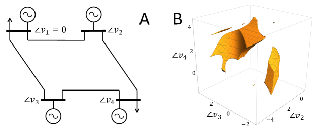
Figure 2. (A) A four bus power system from [75] with two loads and four generators. (B) Feasible region of voltage angles, in which demand and technological constraints of AC formulation are satisfied.

In the AC model, characteristics of the network in a time interval $t\in\mathcal{T}$, can be described by a triplet of admittance matrices $\vec{\mathbf{Y}}_{t},\mathchoice{\mkern 3.0mu\reflectbox{$\displaystyle\vec{\reflectbox{$\mkern-3.0mu\displaystyle\mathbf{Y}\mkern 3.0mu$}}$}\mkern-3.0mu}{\mkern 3.0mu\reflectbox{$\textstyle\vec{\reflectbox{$\mkern-3.0mu\textstyle\mathbf{Y}\mkern 3.0mu$}}$}\mkern-3.0mu}{\mkern 2.0mu\reflectbox{$\scriptstyle\vec{\reflectbox{$\mkern-2.0mu\scriptstyle\mathbf{Y}\mkern 2.0mu$}}$}\mkern-2.0mu}{\mkern 2.0mu\reflectbox{$\scriptscriptstyle\vec{\reflectbox{$\mkern-2.0mu\scriptscriptstyle\mathbf{Y}\mkern 2.0mu$}}$}\mkern-2.0mu}_{t}\in\mathbb{C}^{\mathcal{E}_{t}\times\mathcal{V}}$ and $\mathbf{Y}_{t}\in\mathbb{C}^{\mathcal{V}\times\mathcal{V}}$, that govern the flow of power throughout the network. Next, we define the family $\{\mathcal{N}^{\mathrm{AC}}_{t}\}_{t\in\mathcal{T}}$ and give a brief description for each constraint.

Definition 2.

For every time interval $t\in\mathcal{T}$, let $\mathcal{N}^{\mathrm{AC}}_{t}$ be the set of pairs $(\mathbf{p}_{\bullet,t},\mathbf{q}_{\bullet,t})\in\mathbb{R}^{T\times 2}$, for which there exists a vector of complex voltages $\mathbf{v}_{\bullet,t}\in\mathbb{C}^{\mathcal{V}}$ satisfying the constraints [7a]–[7d].

AC Power Balance Equation:

Constraint [7a] is referred to as the power balance equation which accounts for the conservation of energy at all buses of the network. The vector $\mathbf{d}_{t}\in\mathbb{C}^{\mathcal{N}}$ denotes the demand forecast at each bus, in interval $t$, whose real and imaginary parts account for active and reactive power demands, respectively. Observe that the overall complex power produced by generating units located at each bus $k\in\mathcal{V}$ is given by the $k$-th entry of $\mathbf{C}^{\top}(\mathbf{p}_{\bullet t}+i\mathbf{q}_{\bullet t})$. Finally, the $k$-th entry of the vector $\mathrm{diag}\{\mathbf{v}_{\bullet,t}\mathbf{v}^{\ast}_{\bullet,t}\mathbf{Y}^{\ast}_{t}\}$ is equal to the amount of complex power exchange between bus $k$ and the rest of the network. The voltages across the network are adjusted in such a way that the overall complex power produced at each bus equals the sum of power consumptions and power exchanges of that bus, at all times. This requirement is enforces by constraint [7a].

AC Thermal Limits:

Due to thermal losses, the flow entering a line may differ from the flow leaving the line at the other end. For each time interval $t\in\mathcal{T}$, complex power flows entering the lines of the network through their starting and ending buses are given by vectors $\mathrm{diag}\{\vec{\mathbf{C}}_{t}\mathbf{v}_{\bullet,t}\mathbf{v}^{\ast}_{\bullet,t}\vec{\mathbf{Y}}_{t}^{\ast}\}$ and $\mathrm{diag}\{\mathchoice{\mkern 3.0mu\reflectbox{$\displaystyle\vec{\reflectbox{$\mkern-3.0mu\displaystyle\mathbf{C}\mkern 3.0mu$}}$}\mkern-3.0mu}{\mkern 3.0mu\reflectbox{$\textstyle\vec{\reflectbox{$\mkern-3.0mu\textstyle\mathbf{C}\mkern 3.0mu$}}$}\mkern-3.0mu}{\mkern 2.0mu\reflectbox{$\scriptstyle\vec{\reflectbox{$\mkern-2.0mu\scriptstyle\mathbf{C}\mkern 2.0mu$}}$}\mkern-2.0mu}{\mkern 2.0mu\reflectbox{$\scriptscriptstyle\vec{\reflectbox{$\mkern-2.0mu\scriptscriptstyle\mathbf{C}\mkern 2.0mu$}}$}\mkern-2.0mu}_{t}\mathbf{v}_{\bullet,t}\mathbf{v}^{\ast}_{\bullet,t}\mathchoice{\mkern 3.0mu\reflectbox{$\displaystyle\vec{\reflectbox{$\mkern-3.0mu\displaystyle\mathbf{Y}\mkern 3.0mu$}}$}\mkern-3.0mu}{\mkern 3.0mu\reflectbox{$\textstyle\vec{\reflectbox{$\mkern-3.0mu\textstyle\mathbf{Y}\mkern 3.0mu$}}$}\mkern-3.0mu}{\mkern 2.0mu\reflectbox{$\scriptstyle\vec{\reflectbox{$\mkern-2.0mu\scriptstyle\mathbf{Y}\mkern 2.0mu$}}$}\mkern-2.0mu}{\mkern 2.0mu\reflectbox{$\scriptscriptstyle\vec{\reflectbox{$\mkern-2.0mu\scriptscriptstyle\mathbf{Y}\mkern 2.0mu$}}$}\mkern-2.0mu}_{t}^{\ast}\}$, respectively. Constraints [7b] and [7c] restrict the flow of power, within the thermal limit of the lines $\mathbf{f}_{\mathrm{max};t}\in\mathbb{R}^{\mathcal{L}_{t}}$, for each $t\in\mathcal{T}$.

Voltage Magnitude Limits:

In order for power system components to operate properly, the voltage magnitude at each bus needs to remain within a prespecified range, given by vectors $\mathbf{v}_{\mathrm{min}},\mathbf{v}_{\mathrm{max}}\in\mathbb{R}^{\mathcal{V}}$. Voltage magnitude limits are enforced through the constraint [7d].

The nonlinear AC network constraints [7a]–[7d] pose a significant challenge for solving power system optimization problems based on a full model. As a result, typically a simplified version of the AC model is considered in practice which is explained next.

0.7.2. Direct Current Power Flow Model

The DC model can be formulated by ignoring the reactive powers, voltage magnitude deviations from their nominal values, and network losses. Under this model, the network is described by means of sustenance matrices $\vec{\mathbf{B}}_{t}\in\mathbb{R}^{\mathcal{E}_{t}\times\mathcal{V}}$ and $\mathbf{B}_{t}\in\mathbb{R}^{\mathcal{V}\times\mathcal{V}}$. Moreover, the flow of active power across the network in each time interval $t\in\mathcal{T}$ is expressed with respect to the vector of voltage angles $\boldsymbol{\theta}_{\bullet,t}\in\mathbb{R}^{\mathcal{V}}$.

Definition 3.

For every time interval $t\in\mathcal{T}$, let $\mathcal{N}^{\mathrm{DC}}_{t}$ be the set of pairs $(\mathbf{p}_{\bullet,t},\mathbf{q}_{\bullet,t})\in\mathbb{R}^{T\times 2}$, for which there exists a vector of voltage phase values $\boldsymbol{\theta}_{\bullet,t}\in\mathbb{R}^{\mathcal{V}}$ satisfying constraints [8a]–[8c].

Constraint [8b] is a simplified alternative for power balance equation [7a], in which the vector $\mathbf{B}_{t}\boldsymbol{\theta}_{\bullet,t}\in\mathbb{R}^{\mathcal{V}}$ contains approximate values for active power exchanges between each vertex and the rest of the network. Additionally, thermal limits are enforced through the constraint [8c], in which $\vec{\mathbf{B}}_{t}\boldsymbol{\theta}_{\bullet,t}\in\mathbb{R}^{\mathcal{L}_{t}}$ is the vector of approximate values for active power flow of lines. Notice that, since the network losses are ignored under the DC model, power flows entering both directions are considered equal and it suffices to enforce one inequality for each line.

Methodology

In order to tackle a general power system scheduling problem of the form [1a]–[1c], we develop third-order semidefinite programming (TSDP) relaxations for the families of sets $\{\mathcal{U}_{g}\}_{g\in\mathcal{G}}$ and $\{\mathcal{N}_{t}\}_{t\in\mathcal{T}}$, which lead to a computationally-tractable algorithm. The proposed approach involves introducing additional variables, each as a proxy for a quadratic monomial. We design a class of inequalities, to strengthening the relation between each proxy variable and the monomial it represents.

$$\!\!\!\!\!\!\!\left(\!\!\begin{bmatrix}&+1&\\ 1&-1&\\ &&+1\\ 1&&-1\end{bmatrix}\!\!\otimes\!\!\begin{bmatrix}&-\underaccent{\bar}{p}_{g}&&+1&\\ &+\bar{p}_{g}&&-1&\\ &&-\underaccent{\bar}{p}_{g}&&+1\\ &&+\bar{p}_{g}&&-1\\ s_{g}&r_{g}\!-\!s_{g}&&+1&-1\\ s_{g}&&r_{g}\!-\!s_{g}&-1&+1\\ \end{bmatrix}\right)\!\!\times\!\!\begin{bmatrix}\mathbf{e}^{\top}_{1}\\ \mathbf{e}^{\top}_{2}\!\!+\!\mathbf{e}^{\top}_{6}\!\!+\!\mathbf{e}^{\top}_{7}\\ \mathbf{e}^{\top}_{3}\!\!+\!\mathbf{e}^{\top}_{11}\!\!+\!\mathbf{e}^{\top}_{13}\\ \mathbf{e}^{\top}_{4}\!+\!\mathbf{e}^{\top}_{9}\\ \mathbf{e}^{\top}_{5}\!+\!\mathbf{e}^{\top}_{15}\\ \mathbf{e}^{\top}_{8}\!+\!\mathbf{e}^{\top}_{12}\\ \mathbf{e}^{\top}_{14}\\ \mathbf{e}^{\top}_{10}\end{bmatrix}^{\!\!\top}\!\!\!\!\times\!\!\begin{bmatrix}1\\ x_{g,t-1}\\ x_{g,t}\\ p_{g,t-1}\\ p_{g,t}\\ u_{g,t}\\ y_{g,t}\\ z_{g,t}\end{bmatrix}\!\!\geq\!0,\!\!\!\!$$ (9a)

$$\!\!\!\!\!\!\!\left(\begin{bmatrix}&+1&\\ 1&-1&\\ &+\bar{p}_{g}&-1\\ &-\underaccent{\bar}{p}_{g}&+1\end{bmatrix}\!\!\otimes\!\!\begin{bmatrix}+1\\ -1\\ +1\\ -1\end{bmatrix}^{\!\!\top}\right)\!\!\times\!\!\begin{bmatrix}\dot{\mathbf{e}}^{\top}_{1}\\ \dot{\mathbf{e}}^{\top}_{2}\\ \dot{\mathbf{e}}^{\top}_{3}+\dot{\mathbf{e}}^{\top}_{5}+\dot{\mathbf{e}}^{\top}_{7}\!\!\\ \dot{\mathbf{e}}^{\top}_{4}\\ \dot{\mathbf{e}}^{\top}_{6}\\ \dot{\mathbf{e}}^{\top}_{8}\\ \dot{\mathbf{e}}^{\top}_{9}+\dot{\mathbf{e}}^{\top}_{11}\\ \dot{\mathbf{e}}^{\top}_{10}\\ \dot{\mathbf{e}}^{\top}_{12}\end{bmatrix}^{\top}\times\begin{bmatrix}1\\ x_{g,t-2}\\ x_{g,t-1}\\ x_{g,t}\\ u_{g,t-1}\\ u_{g,t}\\ p_{g,t-1}\\ z_{g,t-1}\\ y_{g,t}\end{bmatrix}\geq 0,$$ (9b)

$$\!\!\!\!\!\!\!\left(\begin{bmatrix}&+1&\\ 1&-1&\\ &+\bar{p}_{g}&-1\\ &-\underaccent{\bar}{p}_{g}&+1\end{bmatrix}\!\!\otimes\!\!\begin{bmatrix}-1\\ +1\\ -1\end{bmatrix}^{\top}\right)\!\!\times\!\!\begin{bmatrix}\ddot{\mathbf{e}}^{\top}_{1}\\ \ddot{\mathbf{e}}^{\top}_{2}+\ddot{\mathbf{e}}^{\top}_{5}\\ \ddot{\mathbf{e}}^{\top}_{3}\\ \ddot{\mathbf{e}}^{\top}_{4}\\ \ddot{\mathbf{e}}^{\top}_{6}\\ \ddot{\mathbf{e}}^{\top}_{8}\\ \ddot{\mathbf{e}}^{\top}_{7}\\ \ddot{\mathbf{e}}^{\top}_{9}\end{bmatrix}^{\top}\!\!\times\!\begin{bmatrix}x_{g,t-2}\\ x_{g,t-1}\\ x_{g,t}\\ u_{g,t-1}\\ u_{g,t}\\ p_{g,t-1}\\ z_{g,t-1}\\ y_{g,t}\end{bmatrix}\geq 0.$$ (9c)

$$\otimes \left\{\mathbf{e}_{1},\mathbf{e}_{2},\ldots,\mathbf{e}_{15}\right\} \left\{\dot{\mathbf{e}}_{1},\dot{\mathbf{e}}_{2},\ldots,\dot{\mathbf{e}}_{12}\right\} \left\{\ddot{\mathbf{e}}_{1},\ddot{\mathbf{e}}_{2},\ldots,\ddot{\mathbf{e}}_{9}\right\} \mathbb{R}^{15} \mathbb{R}^{12} \mathbb{R}^{9}$$ denotes the Kronecker product of two matrices. , and denote the standard basis vectors for , , and , respectively.

In this work, we propose a convex relaxation of the power system scheduling problem [1a]–[1c], which is built by substituting the unit and AC network feasible sets with their convex surrogates $\{\mathcal{U}^{\mathrm{TSDP}}_{g}\}_{g\in\mathcal{G}}$ and $\{\mathcal{N}^{\mathrm{TSDP}}_{t}\}_{t\in\mathcal{T}}$, respectively:

$$\underset{\begin{subarray}{c}\\ \mathbf{x},\mathbf{p},\mathbf{q},\mathbf{c}\in\mathbb{R}^{G\!\times\!T}\!\!\!\!\!\!\!\!\!\!\end{subarray}}{\text{minimize}} \sum_{g=1}^{G}{\sum_{t=1}^{T}{c_{g,t}}}$$ (10a)

subject to $$(\mathbf{x}^{\top}_{g,\bullet},\mathbf{p}^{\top}_{g,\bullet},\mathbf{q}^{\top}_{g,\bullet},\mathbf{c}^{\top}_{g,\bullet})\in\mathcal{U}^{\mathrm{TSDP}}_{g} \forall g\in\mathcal{G},$$ (10b)

$$(\mathbf{p}_{\bullet,t},\mathbf{q}_{\bullet,t})\in\mathcal{N}^{\mathrm{TSDP}}_{t} \forall t\in\mathcal{T},$$ (10c)

Due to convexity of the sets $\{\mathcal{U}^{\mathrm{TSDP}}_{g}\}_{g\in\mathcal{G}}$ and $\{\mathcal{N}^{\mathrm{TSDP}}_{t}\}_{t\in\mathcal{T}}$, the problem [10a]–[10c] can be solved in polynomial time. Moreover, since $\mathcal{U}_{g}\subseteq\mathcal{U}^{\mathrm{TSDP}}_{g}$ and $\mathcal{N}^{\mathrm{AC}}_{t}\subseteq\mathcal{N}^{\mathrm{TSDP}}_{t}$, for every $g\in\mathcal{G}$ and $t\in\mathcal{T}$, respectively, the optimal cost of problem [10a]–[10c] is a lower bound to the optimal cost of problem [1a]–[1c]. If an optimal solution to the problem [10a]–[10c] satisfies the original constraints [1b] and [1c], then the relaxation is exact and a provably global optimal solution to problem [1a]–[1c] is obtained. Otherwise, a rounding procedure is adopted to transform the optimal solution of [10a]–[10c] to a feasible and near optimal solution of [1a]–[1c].

0.8. Relaxation of Unit Constraints

Each unit feasible set $\mathcal{U}_{g}$ is a semialgebraic set, with constraints [2] and [3] as the sources of nonconvexity. In this work, we create a family of convex surrogates $\{\mathcal{U}^{\mathrm{TSDP}}_{g}\}_{g\in\mathcal{G}}$, by enforcing a collection of linear and conic inequalities. To this end, define auxiliary variables $\mathbf{u},\mathbf{y},\mathbf{z},\mathbf{o}\in\mathbb{R}^{G\times T}$, whose components account for monomials $x_{g,t-1}x_{g,t}$, $p_{g,t-1}x_{g,t}$, $x_{g,t-1}p_{g,t}$ and $p^{2}_{g,t}$, respectively. In other words, if the relaxation is exact, the equations

$$u_{g,t}=x_{g,t-1}x_{g,t},\quad y_{g,t}=p_{g,t-1}x_{g,t},$$ (11a)

$$z_{g,t}=x_{g,t-1}p_{g,t},\quad P_{g,t}=p^{2}_{g,t},$$ (11b)

hold true at optimality. To capture the binary requirement for commitment decisions, the following convex inequalities, that are referred to as “McCormick constraints”, are enforced:

$$\max\{0,x_{g,t-1}+x_{g,t}-1\}\leq u_{g,t}\leq\min\{x_{g,t-1},x_{g,t}\}.$$ (12)

Now, constraint [3] can be cast in the following linear form, with respect to the auxiliary variables:

$$c_{g,t}=\alpha_{g}o_{g,t}+\beta_{g}p_{g,t}+$$

$$\quad\quad\;\;\,\gamma_{g}x_{g,t}+\gamma_{g}^{\uparrow}(x_{g,t}-u_{g,t})+\gamma_{g}^{\downarrow}(x_{g,t-1}-u_{g,t}).$$ (13)

Finally, we relax the nonconvex equations [11a]–[11b] with the following conic constraints:

[14,14]

as well as a number of linear inequalities that are stated next.

Definition 4.

For each $g\in\mathcal{G}$, define $\mathcal{U}^{\mathrm{TSDP}}_{g}\subset\mathbb{R}^{T\times 4}$ to be the set of all quadruplets $(\mathbf{x}^{\top}_{g,\bullet},\mathbf{p}^{\top}_{g,\bullet},\mathbf{q}^{\top}_{g,\bullet},\mathbf{c}^{\top}_{g,\bullet})$, for which there exists $(\mathbf{u}^{\top}_{g,\bullet},\mathbf{y}^{\top}_{g,\bullet},\mathbf{z}^{\top}_{g,\bullet},\mathbf{o}^{\top}_{g,\bullet})\in\mathbb{R}^{T\times 4}$, such that for every $t\in\mathcal{T}$, the following constraints hold true:

• The linear inequalities [4], [5], [6],

• The conic and linear constraints [12], [13], [14], [14] and [9a],

• The linear inequalities [9b], if $m^{\downarrow}_{g}>1$,

• The linear inequalities [9c], if $m^{\uparrow}_{g}>1$.

Notice that for each $g\in\mathcal{G}$, the relaxed feasible set $\mathcal{U}^{\mathrm{TSDP}}_{g}$ is defined, by means of conic and linear inequalities that are convex. The validity of these inequalities is proven in SI Text.

The definition of $\mathcal{U}^{\mathrm{TSDP}}_{g}$ involves $2\times T$ third-order semidefinite constraints that can be enforced efficiently. Additionally, the overall number of inequalities grows linearly with respect to $T$, which is an improvement upon existing methods. On the other hand, the ramp and minimum up & down constraints are incorporated into the valid inequalities, the present convex relaxation offers more accurate bounds, in the case of severe load variations.

0.9. Relaxation of Network Constraints

A state of the art method, given in [66], for convex relaxation of AC power flow equations incorporates an auxiliary matrix variable $\mathbf{W}_{t}\in\mathbb{H}_{n}$, for each $t\in\mathcal{T}$, accounting for $\mathbf{v}_{\bullet,t}\mathbf{v}^{\ast}_{\bullet,t}$. Using the matrix $\mathbf{W}_{t}\in\mathbb{H}_{n}$, the AC network constraints [7a]–[7d] can be convexified as follows:

$$\mathbf{d}_{t}+\mathrm{diag}\{\mathbf{W}_{t}\;\mathbf{Y}^{\ast}_{t}\} =\mathbf{C}^{\top}(\mathbf{p}_{\bullet t}+i\mathbf{q}_{\bullet t})$$ (15a)

$$\lvert\mathrm{diag}\{\vec{\mathbf{C}}_{t}\;\mathbf{W}_{t}\;\vec{\mathbf{Y}}_{t}^{\ast}\}\rvert \leq\mathbf{f}_{\mathrm{max};t}$$ (15b)

$$\lvert\mathrm{diag}\{\mathchoice{\mkern 3.0mu\reflectbox{$\displaystyle\vec{\reflectbox{$\mkern-3.0mu\displaystyle\mathbf{C}\mkern 3.0mu$}}$}\mkern-3.0mu}{\mkern 3.0mu\reflectbox{$\textstyle\vec{\reflectbox{$\mkern-3.0mu\textstyle\mathbf{C}\mkern 3.0mu$}}$}\mkern-3.0mu}{\mkern 2.0mu\reflectbox{$\scriptstyle\vec{\reflectbox{$\mkern-2.0mu\scriptstyle\mathbf{C}\mkern 2.0mu$}}$}\mkern-2.0mu}{\mkern 2.0mu\reflectbox{$\scriptscriptstyle\vec{\reflectbox{$\mkern-2.0mu\scriptscriptstyle\mathbf{C}\mkern 2.0mu$}}$}\mkern-2.0mu}_{t}\;\mathbf{W}_{t}\;\mathchoice{\mkern 3.0mu\reflectbox{$\displaystyle\vec{\reflectbox{$\mkern-3.0mu\displaystyle\mathbf{Y}\mkern 3.0mu$}}$}\mkern-3.0mu}{\mkern 3.0mu\reflectbox{$\textstyle\vec{\reflectbox{$\mkern-3.0mu\textstyle\mathbf{Y}\mkern 3.0mu$}}$}\mkern-3.0mu}{\mkern 2.0mu\reflectbox{$\scriptstyle\vec{\reflectbox{$\mkern-2.0mu\scriptstyle\mathbf{Y}\mkern 2.0mu$}}$}\mkern-2.0mu}{\mkern 2.0mu\reflectbox{$\scriptscriptstyle\vec{\reflectbox{$\mkern-2.0mu\scriptscriptstyle\mathbf{Y}\mkern 2.0mu$}}$}\mkern-2.0mu}_{t}^{\ast}\}\rvert \leq\mathbf{f}_{\mathrm{max};t}$$ (15c)

$$\mathbf{v}_{\mathrm{min}}\leq\lvert\mathrm{diag}\{\mathbf{W}_{t}\}\rvert \leq\mathbf{v}_{\mathrm{max}}$$ (15d)

In formulation [15a]–[15d], the structure of matrix $\mathbf{W}_{t}$, i.e.,

$$\mathbf{W}_{t}=\mathbf{v}_{\bullet,t}\mathbf{v}^{\ast}_{\bullet,t}$$ (16)

is ignored, to make the model polynomially solvable. To remedy the absence of the non-convex equation [16], the relaxation can be strengthened through a combination of conic constraints, with the aim of enforcing the relation between $\mathbf{W}_{t}$ and $\mathbf{v}_{\bullet,t}$, implicitly.

Observe that an arbitrary matrix $\mathbf{W}_{t}\in\mathbb{H}_{n}$ can be factored to $\mathbf{v}_{\bullet,t}\mathbf{v}^{\ast}_{\bullet,t}$, if and only if, it is rank-one and positive semidefinite:

$$\mathrm{rank}\{\mathbf{W}_{t}\}=1\quad\wedge\quad\mathbf{W}_{t}\succeq 0.$$ (17)

Although a rank constraint on $\mathbf{W}_{t}$ cannot be enforced efficiently, employing the convex constraint $\mathbf{W}_{t}\succeq 0$ leads to the semidefinite programming (SDP) relaxation of AC network constraints. For larger-scale systems, a graph-theoretic analysis divides the set of buses into several overlapping subsets $\mathcal{A}_{1},\mathcal{A}_{2},\ldots,\mathcal{A}_{A}\subseteq\mathcal{V}$, such that the relaxation could be represented with smaller conic constraints:

$$\mathbf{W}_{t}[\mathcal{A}_{k},\mathcal{A}_{k}]\succeq 0,\qquad\forall k\in\{1,2,\ldots,A\},$$ (18)

where for every $\mathcal{X}\subseteq\{1,\ldots,n\}$, the notation $\mathbf{W}_{t}[\mathcal{X},\mathcal{X}]$ represents the $|\mathcal{X}|\times|\mathcal{X}|$ principal submatrix of $\mathbf{W}_{t}$, whose rows and columns are chosen from $\mathcal{X}$. Choosing $\mathcal{A}_{1},\mathcal{A}_{2},\ldots,\mathcal{A}_{A}$, based on the bags of an arbitrary tree decomposition of the network, leads to an equivalent but more efficient SDP relaxation [66]. A weaker, but far more tractable approach is the second-order cone programming (SOCP) relaxation which uses conic constraints of the following form:

$$\begin{bmatrix}W_{k_{1},k_{1}}\!&\!\!W_{k_{1},k_{2}}\!\\ W_{k_{2},k_{1}}\!&\!\!W_{k_{2},k_{2}}\!\end{bmatrix}\!\succeq 0,\qquad\forall(k_{1},k_{2})\in\mathcal{E}_{t}$$ (19)

To achieve a better balance between the strength of the convex relaxation and scalability, in this paper, we use a third-order semidefinite programming (TSDP) relaxation which is described as follows:

Definition 5.

For each $t\in\mathcal{T}$, let $\mathcal{N}^{\mathrm{TSDP}}_{t}\subset\mathbb{R}^{G\times 2}$ be the set of pairs $(\mathbf{p}^{\top}_{g,\bullet},\mathbf{q}^{\top}_{g,\bullet})$, for which there exists a Hermitian matrix $\mathbf{W}_{t}\in\mathbb{H}_{n}$, that satisfies constraints [15a]–[15d] and the following third-order semidefinite constraints

$$\begin{bmatrix}W_{k_{1},k_{1}}\!&\!\!W_{k_{1},k_{2}}\!&\!\!W_{k_{1},k_{3}}\\ W_{k_{2},k_{1}}\!&\!\!W_{k_{2},k_{2}}\!&\!\!W_{k_{2},k_{3}}\\ W_{k_{3},k_{1}}\!&\!\!W_{k_{3},k_{2}}\!&\!\!W_{k_{3},k_{3}}\end{bmatrix}\!\succeq 0,$$ (20)

for every $(k_{1},k_{2},k_{3})\in\bigcup_{k=1}^{A}\mathcal{A}_{k}\times\mathcal{A}_{k}\times\mathcal{A}_{k}$, where $\mathcal{A}_{1},\mathcal{A}_{2},\ldots,\mathcal{A}_{A}\subseteq\mathcal{V}$, are the bags associated with an arbitrary tree decomposition of the network $\mathcal{H}_{t}$, for which $|\mathcal{A}_{k}|\geq 3$, $\forall k\in\{1,\ldots A\}$.

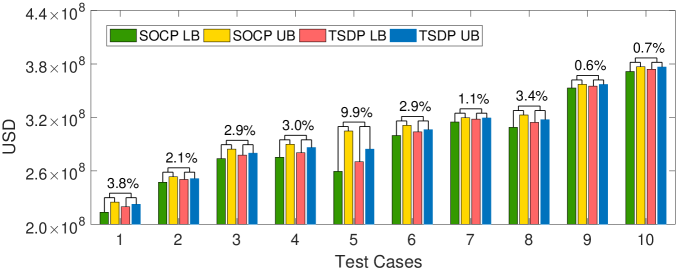
Figure 3. Comparisons between the performance of TSDP and SOCP relaxations of the AC network constraints on ten instances of PEGASE 1354-bus system. The difference between optimality gaps are shown.

Comparison of the models

We have compared the performance of the proposed TSDP relaxation (Definition 5) with the SOCP relaxation given by [19] in terms of: i) upper bound (UB) given by the cost of the feasible solution returned and; ii) convex lower bound (LB) on the optimal cost. To that end, ten instances based on each European system in Table 1 are considered. In all instances of the largest PEGASE 2869-bus, 9241-bus and 13659-bus cases, the Newton-Raphson’s local search method successfully converges to a feasible operating point when started with an initial point from TSDP relaxation (discussed in detail in Section Recovering a Feasible Solution); however, it fails to converge when started with points from the SOCP relaxation. For the instances on the smallest PEGASE 1354-bus system, both SOCP and TSDP relaxations lead to feasible solutions through Newton-Raphson’s local search. Figure 3 displays the optimal relaxation objective value (LB) and the cost of the resulting feasible solution (UB) for this system. Although very fast to solve, the SOCP relaxation is substantially worse than the TSDP relaxation, as seen in Figure 3. Motivated by the aforementioned observation, we propose the TSDP relaxation to convexify the AC network equations [7a]–[7d], in power system scheduling.

Discussion and Conclusions

In this paper, we study the problem of optimizing grids operation throughout a planning horizon, based on the available resources for supply and transmission of electricity. This fundamental problem is heavily investigated for decades and need to be solved on a daily basis by independent system operators and utility companies. The challenge is twofold: first, determining a massive number of highly correlated binary decisions that account for commitment of generators; secondly, finding the most economic transmission strategy in accordance with laws of physics and technological limitations.

We propose a third-order semidefinite programming (TSDP) method that is equipped with an accurate physical model for the flow of electricity and offers massive scalability in the number of generating units and grid size. While co-optimization of supply and transmission under the full physical model has long been put forward as a direction to boost the efficiency and reliability of operation, scalability has been the main bottleneck to-date. Significant improvement over the state-of-the-art methods is validated on day-ahead grid scheduling problems, on the largest publicly available real-world data.

Given the simplicity of the linear algebraic operations on 3x3 Hermitian matrices, a direction of interest is to build a highly parallel numerical algorithm for solving large-scale TSDP problems on graphical processing units high-performance computing facilitates.

Materials and Methods

This section details the procedure for recovering a feasible solution to the scheduling from the optimal solution of the relaxed problem [10a]–[10c] and data generation.

Recovering a Feasible Solution

Let $(\mathbf{x}^{\mathrm{opt}},\mathbf{p}^{\mathrm{opt}},\mathbf{q}^{\mathrm{opt}},\mathbf{c}^{\mathrm{opt}})$ be an optimal solution to the relaxed problem [10a]–[10c]. If all entries of $\mathbf{x}^{\mathrm{opt}}$ turn out to be integer, and there exists a matrix $\mathbf{v}\in\mathbb{C}^{\mathcal{V}\times\mathcal{T}}$ that satisfies constraints [7a]–[7d], then $(\mathbf{x}^{\mathrm{opt}},\mathbf{p}^{\mathrm{opt}},\mathbf{q}^{\mathrm{opt}},\mathbf{c}^{\mathrm{opt}})$ is a globally optimal solution to problem [1a]–[1c]. However, the relaxation is often inexact, and solutions to the relaxed problem [10a]–[10c] are not necessarily feasible for problem [1a]–[1c]. In such cases, a recovery process is needed to transform $(\mathbf{x}^{\mathrm{opt}},\mathbf{p}^{\mathrm{opt}},\mathbf{q}^{\mathrm{opt}},\mathbf{c}^{\mathrm{opt}})$ to a feasible and near-optimal solution for problem [1a]–[1c].

Algorithm 1 Recovering a Feasible Solution

The optimal unit commitment solution $\mathbf{x}^{\mathrm{opt}}\in\mathbb{R}^{G\times T}$ to problem [10a]–[10c]:

for $g=1\ldots,G$ do

    for $t=1-\max\{m^{\uparrow}_{g},m^{\downarrow}_{g}\},\ldots,0$ do

         Set $x^{\mathrm{feas}}_{g,t}$ according to the initial state of unit $g$.

    end for

end for

for $g=1\ldots,G$ do

    for $t=1\ldots,T$ do

         $a^{\uparrow}\!\!\leftarrow\!\max\{x^{\mathrm{feas}}_{g,\tau}-x^{\mathrm{feas}}_{g,\tau-1}\;|\;\forall\tau\!\in\!\{t-m^{\uparrow}_{g}+1,\ldots,t-1\}\}$

         $a^{\downarrow}\!\!\leftarrow\!\max\{x^{\mathrm{feas}}_{g,\tau-1}-x^{\mathrm{feas}}_{g,\tau}\;|\;\forall\tau\!\in\!\{t-m^{\downarrow}_{g}+1,\ldots,t-1\}\}$

         if $a^{\uparrow}=a^{\downarrow}=1$ then

             Declare failure.

         else

             if $a^{\uparrow}=1$ then

                 $x^{\mathrm{feas}}_{g,t}\leftarrow 1$

             end if

             if $a^{\downarrow}=1$ then

                 $x^{\mathrm{feas}}_{g,t}\leftarrow 0$

             end if

             if $a^{\uparrow}=a^{\downarrow}=0$ then

                 $x^{\mathrm{feas}}_{g,t}\leftarrow\mathrm{round}\{x^{\mathrm{opt}}_{g,t}+0.25\}$

             end if

         end if

    end for

end for

return $\mathbf{x}^{\mathrm{feas}}$

As demonstrated by Table 1, on average, only a small portion of the binary variables remain fractional after solving the proposed TSDP relaxation problem. In all of our experiments, a feasible candidate for $\mathbf{x}$ is obtained, through the Algorithm 1, which simply rounds each entry of $\mathbf{x}^{\mathrm{opt}}$ subject to minimum up and down time constraints [5b] and [5a].

Another challenge is finding a feasible voltage profile $\mathbf{v}=[\mathbf{v}_{\bullet,1}|\mathbf{v}_{\bullet,2}|\ldots|\mathbf{v}_{\bullet,T}]\in\mathbb{C}^{\mathcal{V}\times\mathcal{T}},$ based on a solution to the relaxed problem [10a]–[10c]. If the rank constraints [17] are not satisfied at optimality, then the relaxation of network equations is not exact and it is not possible to factorize the resulting matrices $\mathbf{W}^{\mathrm{opt}}_{1},\mathbf{W}^{\mathrm{opt}}_{2},\ldots,$ $\mathbf{W}^{\mathrm{opt}}_{T}$, in the form of equation [16]. A “recovery algorithm” is introduced in [66], for finding an approximate vector of voltages $\hat{\mathbf{v}}_{\bullet,t}$ based on $\mathbf{W}^{\mathrm{opt}}_{t}$, which minimizes the overall mismatch (i.e., violation of network equations). In order to obtain voltage profiles with no mismatch, we feed the outcome of the recovery algorithm from [66] as the initial point to Newton-Raphson’s local search algorithm. This procedure is described next:

1. Find a feasible matrix of commitment decisions $\mathbf{x}^{\mathrm{feas}}$ via Algorithm 1.

2. For every $t=1\ldots,T$:

   1. Obtain an approximate voltage profile $\hat{\mathbf{v}}_{\bullet,t}$ from $\mathbf{W}^{\mathrm{opt}}_{t}$ based on the recovery algorithm in [66].

   2. Start with $\mathbf{p}^{\mathrm{opt}}_{\bullet,t}$, $\mathbf{q}^{\mathrm{opt}}_{\bullet,t}$ and $\hat{\mathbf{v}}_{\bullet,t}$, as the initial point to search locally for a triplet of vectors $\mathbf{p}^{\mathrm{feas}}_{\bullet,t}\in\mathbb{R}^{G}$, $\mathbf{q}^{\mathrm{feas}}_{\bullet,t}\in\mathbb{R}^{G}$ and $\mathbf{v}^{\mathrm{feas}}_{\bullet,t}\in\mathbb{C}^{\mathcal{V}}$, that minimizes the objective function $\sum^{G}_{g=1}{\alpha_{g}p^{2}_{g,t}+\beta_{g}p_{g,t}}$, subject to the constraints [7a]–[7d] and

      $$\underaccent{\bar}{q}_{g}x^{\mathrm{feas}}_{g,t}\leq q_{g,t}\leq\bar{q}_{g}x^{\mathrm{feas}}_{g,t}$$ (21a)

      $$\underaccent{\bar}{p}_{g}x^{\mathrm{feas}}_{g,t}\leq p_{g,t}\leq\bar{p}_{g}x^{\mathrm{feas}}_{g,t}$$ (21b)

      $$p_{g,t}\geq p^{\mathrm{feas}}_{g,t-1}-r_{g}x^{\mathrm{feas}}_{g,t}-s_{g}(1-x^{\mathrm{feas}}_{g,t})$$ (21c)

      $$p_{g,t}\leq p^{\mathrm{feas}}_{g,t-1}+r_{g}x^{\mathrm{feas}}_{g,t-1}+s_{g}(1-x^{\mathrm{feas}}_{g,t-1}).$$ (21d)

   3. Derive the feasible cost values $c^{\mathrm{feas}}_{g,t}$, according to the equation [3].

3. Report $(\mathbf{x}^{\mathrm{feas}},\mathbf{p}^{\mathrm{feas}},\mathbf{q}^{\mathrm{feas}})$ as the output schedule/dispatch and $\mathbf{v}$ as the corresponding voltage profile. The following quantity serves as an upperbound for relative distance from global optimality:

   $$\!\!\mathrm{Gap}\leq 100\times\frac{\sum_{t=1}^{T}{\sum_{g=1}^{G}{(c^{\mathrm{feas}}_{g,t}-c^{\mathrm{opt}}_{g,t})}}}{\sum_{t=1}^{T}{\sum_{g=1}^{G}{c^{\mathrm{feas}}_{g,t}}}}$$ (22)

We have used the procedure described above for the experiments presented in Table 1, and in all cases, a feasible solution could be found within the violation tolerance of the constraint ($10^{-5}$ per-unit).

Data Generation

The network data for IEEE and European systems is obtained from the MATPOWER package [75, 76]. Hourly load changes for the day-ahead at all buses are considered proportional to the numbers reported in [77]. In each experiment, the cost coefficients $\alpha_{g}$, $\beta_{g}$, $\gamma_{g}$, $\gamma^{\downarrow}_{g}$ and $\gamma^{\uparrow}_{g}$ are chosen uniformly between zero and $~{}1~{}\$/(\mathrm{MW.h})^{2}$, $~{}10~{}\$/(\mathrm{MW.h})$, $~{}100~{}\$$, $~{}30~{}\$$ and $~{}50~{}\$$, respectively. The ramp limits of each generating unit are set to $r_{g}=s_{g}=\max\{\bar{p}_{g}/4,\underaccent{\bar}{p}_{g}\}$. For each generating unit, the minimum up and down limits $m^{\uparrow}_{g}$ and $m^{\downarrow}_{g}$ are randomly selected in such a way that $m^{\uparrow}_{g}-1$ and $m^{\downarrow}_{g}-1$ have Poisson distribution with parameter $4$. The initial status of generators at time period $t=0$ is found by solving a single period economic dispatch problem corresponding to the demand at time $t=1$. For each generating unit $g\in\mathcal{G}$, it is assumed that the initial status has been maintained exactly since time period $t=-t^{(0)}_{g}$, where $t^{(0)}_{g}$ has Poisson distribution with parameter $4$. For simplicity, all of the generating units with negative capacity are removed. All simulations are run in MATLAB using a workstation with an Intel 3.0 GHz, 12-core CPU, and 256 GB RAM. The CVX package version 3.0 [78] and MOSEK version 8.0 [79] are used for solving semidefinite programming problems. The data set as well as the log files of the optimization runs are available for download at: http://ieor.berkeley.edu/$\sim$atamturk/data/tsdp.

Acknowledegement

A. Atamtürk is supported, in part, by grant FA9550-10-1-0168 from the Office of the Assistant Secretary of Defense for Research and Engineering.

Appendix

A proof of validity for conic and linear inequalities [14] and [9] is provided in this section.

Proposition 1.

Inequalities [14], [14] and [9a] are valid for every pair of vectors $(\mathbf{x},\mathbf{p})\in\mathbb{R}^{G\times T}$ that satisfy constraints [2], [4a], [6a], [6b], [5a] and [5b]. Additionally, if $m^{\downarrow}_{g}\geq 2$, then constraint [9b] and if $m^{\uparrow}_{g}\geq 2$, then constraint [9c] is valid.

Proof: For every $(g,t)\in\{1,\ldots,G\}\times\{1,\ldots,T\}$, define the vector of monomials:

$$\boldsymbol{\delta}_{g,t}\equiv[ x_{g,t-1},\;x_{g,t},\;p_{g,t-1},\;p_{g,t},$$

$$\underaccent{\bar}{h}_{g,t-1},\;\bar{h}_{g,t-1},\;\underaccent{\bar}{h}_{g,t},\;\bar{h}_{g,t},\;\underaccent{\bar}{a}_{g,t},\;\bar{a}_{g,t},$$

$$x_{g,t-1}\underaccent{\bar}{h}_{g,t-1},\;x_{g,t-1}\bar{h}_{g,t-1},\;x_{g,t-1}\underaccent{\bar}{h}_{g,t},$$

$$x_{g,t-1}\bar{h}_{g,t},x_{g,t-1}\underaccent{\bar}{a}_{g,t},\;x_{g,t-1}\bar{a}_{g,t},$$

$$x_{g,t}\underaccent{\bar}{h}_{g,t-1},\;x_{g,t}\bar{h}_{g,t-1},\;x_{g,t}\underaccent{\bar}{h}_{g,t},$$

$$x_{g,t}\bar{h}_{g,t},\;x_{g,t}\underaccent{\bar}{a}_{g,t},\;x_{g,t}\bar{a}_{g,t}]^{\top},$$ (23)

where

$$\underaccent{\bar}{h}_{g,t} \equiv\sqrt{p_{g,t}-\underaccent{\bar}{p}_{g}x_{g,t}}\;,\qquad\bar{h}_{g,t}\equiv\sqrt{\bar{p}_{g}x_{g,t}-p_{g,t}}\;,$$ (24a)

$$\underaccent{\bar}{a}_{g,t} \equiv\sqrt{s_{g}+(r_{g}-s_{g})x_{g,t-1}+p_{g,t-1}-p_{g,t}}\;,$$ (24b)

$$\bar{a}_{g,t} \equiv\sqrt{s_{g}+(r_{g}-s_{g})x_{g,t}-p_{g,t-1}+p_{g,t}}\;.$$ (24c)

Define $\boldsymbol{\Delta}_{g,t}$ as the $22\times 22$ symmetric matrix formed by multiplying $\boldsymbol{\delta}_{g,t}$ by its transpose:

$$\boldsymbol{\Delta}_{g,t}\equiv\boldsymbol{\delta}_{g,t}\boldsymbol{\delta}_{g,t}^{\top}.$$ (25)

Observe that $\boldsymbol{\Delta}_{g,t}$ is positive semidefinite, and as a consequence, every principle submatrix of $\boldsymbol{\Delta}_{g,t}$ is positive semidefinite, as well. Considering submatrices $\boldsymbol{\Delta}_{g,t}[\{2,1,3\},\{2,1,3\}]$ and $\boldsymbol{\Delta}_{g,t}[\{1,2,4\},\{1,2,4\}]$, concludes the conic constraints [14] and [14], respectively. Moreover, the constraint [9a] encapsulates $24$ linear inequalities, and it is straightforward to verify that inequalities $k$, $k+6$, $k+12$ and $k+18$ can be concluded from

$$\!\!\boldsymbol{\Delta}_{g,t}[\{k+4,k+10,k+16\},\{k+4,k+10,k+16\}]\succeq 0,\!$$ (26)

for each $k=1,2,\ldots,6$. This completes the proof of [9a].

In order to prove the validity constraint [9b], suppose that $m^{\downarrow}_{g}\geq 2$, and consider the following vector of monomials:

$$\boldsymbol{\phi}^{\downarrow}_{g,t}\equiv[ w^{\downarrow}_{g,t},\;x_{g,t-1}w^{\downarrow}_{g,t},\;\underaccent{\bar}{h}_{g,t-1}w^{\downarrow}_{g,t},\;\bar{h}_{g,t-1}w^{\downarrow}_{g,t}]^{\top},$$ (27)

where

$$w^{\downarrow}_{g,t}\equiv\sqrt{1-x_{g,t-2}+x_{g,t-1}-x_{g,t}}\;.$$ (28)

Observe that all four inequalities encapsulated in [9b] can be concluded from the conic inequality $\boldsymbol{\phi}^{\downarrow}_{g,t}(\boldsymbol{\phi}^{\downarrow}_{g,t})^{\top}\succeq 0$.

If $m^{\uparrow}_{g}\geq 2$, the validity of the constraint [9c] can be similarly proven by defining

$$w^{\uparrow}_{g,t}\equiv\sqrt{x_{g,t-2}-x_{g,t-1}+x_{g,t}}\;,$$ (29)

and forming the vector of monomials

$$\boldsymbol{\phi}^{\uparrow}_{g,t}\equiv[ w^{\uparrow}_{g,t},\;x_{g,t-1}w^{\uparrow}_{g,t},\;\underaccent{\bar}{h}_{g,t-1}w^{\uparrow}_{g,t},\;\bar{h}_{g,t-1}w^{\uparrow}_{g,t}]^{\top}.$$ (30)

Finally, the four inequalities from [9c] can be inferred from the conic inequality $\boldsymbol{\phi}^{\uparrow}_{g,t}(\boldsymbol{\phi}^{\uparrow}_{g,t})^{\top}\succeq 0$. ∎

References

- [1] W. Leontief and A. Strout, “Multiregional input-output analysis,” in Structural interdependence and economic development. Springer, 1963, pp. 119–150.
- [2] G. Dantzig, Linear programming and extensions. Princeton university press, 1959.
- [3] M. B. Cain, R. P. O’Neill, and A. Castillo, “History of optimal power flow and formulations,” Federal Energy Regulatory Commission, pp. 1–36, 2012.
- [4] National Academies of Sciences, Engineering, and Medicine and others, Analytic Research Foundations for the Next-Generation Electric Grid. National Academies Press, 2016.
- [5] C. T. Clack, S. A. Qvist, J. Apt, M. Bazilian, A. R. Brandt, K. Caldeira, S. J. Davis, V. Diakov, M. A. Handschy, P. D. Hines et al., “Evaluation of a proposal for reliable low-cost grid power with 100% wind, water, and solar,” Proceedings of the National Academy of Sciences, p. 201610381, 2017.
- [6] G. B. Giannakis, V. Kekatos, N. Gatsis, S.-J. Kim, H. Zhu, and B. F. Wollenberg, “Monitoring and optimization for power grids: A signal processing perspective,” IEEE Signal Processing Magazine, vol. 30, pp. 107–128, 2013.
- [7] P. Lipka, S. S. Oren, R. P. O’Neill, and A. Castillo, “Running a more complete market with the SLP-IV-ACOPF,” IEEE Transactions on Power Systems, vol. 32, pp. 1139–1148, 2017.
- [8] B. Hua and R. Baldick, “A convex primal formulation for convex hull pricing,” IEEE Transactions on Power Systems, vol. PP, pp. 1–1, 2017.
- [9] J. B. Lasserre, “Global optimization with polynomials and the problem of moments,” SIAM Journal on Optimization, vol. 11, pp. 796–817, 2001.
- [10] ——, “Convergent SDP-relaxations in polynomial optimization with sparsity,” SIAM Journal on Optimization, vol. 17, pp. 822–843, 2006.
- [11] M. Laurent, “Sums of squares, moment matrices and optimization over polynomials,” Emerging applications of algebraic geometry, pp. 157–270, 2009.
- [12] J. Gouveia, P. A. Parrilo, and R. R. Thomas, “Theta bodies for polynomial ideals,” SIAM Journal on Optimization, vol. 20, pp. 2097–2118, 2010.
- [13] S. Sojoudi and J. Lavaei, “Exactness of semidefinite relaxations for nonlinear optimization problems with underlying graph structure,” SIAM Journal on Optimization, vol. 24, pp. 1746–1778, 2014.
- [14] P. Belotti, J. C. Góez, I. Pólik, T. K. Ralphs, and T. Terlaky, “A conic representation of the convex hull of disjunctive sets and conic cuts for integer second order cone optimization,” in Numerical Analysis and Optimization. Springer, 2015, pp. 1–35.
- [15] M. Tomamichel, M. Berta, and J. M. Renes, “Quantum coding with finite resources,” Nature communications, vol. 7, 2016.
- [16] S. Nagy and T. Vértesi, “EPR steering inequalities with communication assistance,” Scientific reports, vol. 6, 2016.
- [17] A. Javanmard, A. Montanari, and F. Ricci-Tersenghi, “Phase transitions in semidefinite relaxations,” Proceedings of the National Academy of Sciences, vol. 113, pp. E2218–E2223, 2016.
- [18] E. J. Candes, Y. C. Eldar, T. Strohmer, and V. Voroninski, “Phase retrieval via matrix completion,” SIAM review, vol. 57, pp. 225–251, 2015.
- [19] A. S. Bandeira, “Inference on graphs via semidefinite programming,” Proceedings of the National Academy of Sciences, p. 201603405, 2016.
- [20] Y. Aflalo, A. Bronstein, and R. Kimmel, “On convex relaxation of graph isomorphism,” Proceedings of the National Academy of Sciences, vol. 112, pp. 2942–2947, 2015.
- [21] V. Chandrasekaran and M. I. Jordan, “Computational and statistical tradeoffs via convex relaxation,” Proceedings of the National Academy of Sciences, vol. 110, pp. E1181–E1190, 2013.
- [22] J. Lavaei and S. H. Low, “Zero duality gap in optimal power flow problem,” IEEE Transactions on Power Systems, vol. 27, pp. 92–107, 2012.
- [23] S. Coogan, E. Kim, G. Gomes, M. Arcak, and P. Varaiya, “Offset optimization in signalized traffic networks via semidefinite relaxation,” Transportation Research Part B: Methodological, vol. 100, pp. 82–92, 2017.
- [24] J. Park and S. Boyd, “A semidefinite programming method for integer convex quadratic minimization,” arXiv preprint arXiv:1504.07672, 2015.
- [25] M. Muramatsu and T. Suzuki, “A new second-order cone programming relaxation for max-cut problems,” Journal of the Operations Research Society of Japan, vol. 46, pp. 164–177, 2003.
- [26] S. Kim, M. Kojima, and M. Yamashita, “Second order cone programming relaxation of a positive semidefinite constraint,” Optimization Methods and Software, vol. 18, pp. 535–541, 2003.
- [27] S. Kim and M. Kojima, “Exact solutions of some nonconvex quadratic optimization problems via SDP and SOCP relaxations,” Computational Optimization and Applications, vol. 26, pp. 143–154, 2003.
- [28] X. Bao, N. V. Sahinidis, and M. Tawarmalani, “Semidefinite relaxations for quadratically constrained quadratic programming: A review and comparisons,” Mathematical Programming, vol. 129, pp. 129–157, 2011.
- [29] K. Natarajan, D. Shi, and K.-C. Toh, “A penalized quadratic convex reformulation method for random quadratic unconstrained binary optimization,” Optimization Online, 6 2013.
- [30] E. Allen and M. Ilic, Price-based commitment decisions in the electricity market. Springer Science & Business Media, 2012.
- [31] E. Y. Bitar, R. Rajagopal, P. P. Khargonekar, K. Poolla, and P. Varaiya, “Bringing wind energy to market,” IEEE Transactions on Power Systems, vol. 27, pp. 1225–1235, 2012.
- [32] D. Bertsimas, E. Litvinov, X. A. Sun, J. Zhao, and T. Zheng, “Adaptive robust optimization for the security constrained unit commitment problem,” IEEE Transactions on Power Systems, vol. 28, pp. 52–63, 2013.
- [33] D. T. Phan and A. Koc, “Optimization approaches to security-constrained unit commitment and economic dispatch with uncertainty analysis,” in Optimization and Security Challenges in Smart Power Grids. Springer, 2013, pp. 1–37.
- [34] Y. Yu and R. Rajagopal, “The impacts of electricity dispatch protocols on the emission reductions due to wind power and carbon tax,” Environmental Science & Technology, vol. 49, pp. 2568–2576, 2015.
- [35] A. Lorca and X. Sun, “Multistage robust unit commitment with dynamic uncertainty sets and energy storage,” IEEE Transactions on Power Systems, vol. 32, pp. 1678–1688, May 2017.
- [36] B. Zhao, A. J. Conejo, and R. Sioshansi, “Unit commitment under gas-supply uncertainty and gas-price variability,” IEEE Transactions on Power Systems, vol. 32, pp. 2394–2405, May 2017.
- [37] K. Sundar, H. Nagarajan, L. Roald, S. Misra, R. Bent, and D. Bienstock, “A modified benders decomposition for chance-constrained unit commitment with N-1 security and wind uncertainty,” arXiv preprint arXiv:1703.05206, 2017.
- [38] X. Bai and H. Wei, “Semi-definite programming-based method for security-constrained unit commitment with operational and optimal power flow constraints,” IET Generation, Transmission & Distribution, vol. 3, pp. 182–197, 2009.
- [39] A. Castillo, C. Laird, C. A. Silva-Monroy, J.-P. Watson, and R. P. O’Neill, “The unit commitment problem with AC optimal power flow constraints,” IEEE Transactions on Power Systems, vol. 31, pp. 4853–4866, 2016.
- [40] K. W. Hedman, M. C. Ferris, R. P. O’Neill, E. B. Fisher, and S. S. Oren, “Co-optimization of generation unit commitment and transmission switching with N-1 reliability,” IEEE Transactions on Power Systems, vol. 25, pp. 1052–1063, 2010.
- [41] H. Wu, M. Shahidehpour, and M. E. Khodayar, “Hourly demand response in day-ahead scheduling considering generating unit ramping cost,” IEEE Transactions on Power Systems, vol. 28, pp. 2446–2454, 2013.
- [42] P. Y. Kerl, W. Zhang, J. B. Moreno-Cruz, A. Nenes, M. J. Realff, A. G. Russell, J. Sokol, and V. M. Thomas, “New approach for optimal electricity planning and dispatching with hourly time-scale air quality and health considerations,” Proceedings of the National Academy of Sciences, vol. 112, pp. 10 884–10 889, 2015.
- [43] A. Subramanian, M. J. Garcia, D. S. Callaway, K. Poolla, and P. Varaiya, “Real-time scheduling of distributed resources,” IEEE Transactions on Smart Grid, vol. 4, pp. 2122–2130, 2013.
- [44] J. Ostrowski, M. F. Anjos, and A. Vannelli, “Tight mixed integer linear programming formulations for the unit commitment problem,” IEEE Transactions on Power Systems, vol. 27, pp. 39–46, 2012.
- [45] J. Lee, J. Leung, and F. Margot, “Min-up/min-down polytopes,” Discrete Optimization, vol. 1, pp. 77–85, 2004.
- [46] P. Damcı-Kurt, S. Küçükyavuz, D. Rajan, and A. Atamtürk, “A polyhedral study of production ramping,” Mathematical Programming, vol. 158, pp. 175–205, 2016.
- [47] Z. Geng, A. Conejo, and Q. Xia, “Alternative linearizations for the operating cost function of unit commitment problems,” IET Generation, Transmission & Distribution, 2017.
- [48] M. S. Aktürk, A. Atamtürk, and S. Gürel, “A strong conic quadratic reformulation for machine-job assignment with controllable processing times,” Operations Research Letters, vol. 37, pp. 187–191, 2009.
- [49] A. Frangioni and C. Gentile, “A computational comparison of reformulations of the perspective relaxation: SOCP vs. cutting planes,” Operations Research Letters, vol. 37, pp. 206–210, 2009.
- [50] R. Jabr, “Rank-constrained semidefinite program for unit commitment,” International Journal of Electrical Power & Energy Systems, vol. 47, pp. 13–20, 2013.
- [51] S. Fattahi, M. Ashraphijuo, J. Lavaei, and A. Atamtürk, “Conic relaxations of the unit commitment problem,” To appear in Energy, 2017. [Online]. Available: http://www.sciencedirect.com/science/article/pii/S0360544217310666
- [52] A. Kargarian, Y. Fu, and Z. Li, “Distributed security-constrained unit commitment for large-scale power systems,” IEEE Transactions on Power Systems, vol. 30, pp. 1925–1936, 2015.
- [53] A. Papavasiliou, S. S. Oren, and B. Rountree, “Applying high performance computing to transmission-constrained stochastic unit commitment for renewable energy integration,” IEEE Transactions on Power Systems, vol. 30, pp. 1109–1120, 2015.
- [54] A. Papavasiliou and S. S. Oren, “A comparative study of stochastic unit commitment and security-constrained unit commitment using high performance computing,” in Control Conference (ECC), 2013 European. IEEE, 2013, pp. 2507–2512.
- [55] R. Baldick, U. Helman, B. F. Hobbs, and R. P. O’Neill, “Design of efficient generation markets,” Proceedings of the IEEE, vol. 93, pp. 1998–2012, 2005.
- [56] B. Zhang and D. Tse, “Geometry of injection regions of power networks,” IEEE Transactions on Power Systems, vol. 28, pp. 788–797, 2013.
- [57] B. Kocuk, S. S. Dey, and X. A. Sun, “Inexactness of SDP relaxation and valid inequalities for optimal power flow,” IEEE Transactions on Power Systems, vol. 31, pp. 642–651, 2016.
- [58] C. Coffrin, H. Hijazi, and P. Van Hentenryck, “Strengthening the SDP relaxation of AC power flows with convex envelopes, bound tightening, and valid inequalities,” IEEE Transactions on Power Systems, 2016.
- [59] C. Chen, A. Atamtürk, and S. S. Oren, “Bound tightening for the alternating current optimal power flow problem,” IEEE Transactions on Power Systems, vol. 31, pp. 3729–3736, 2016.
- [60] ——, “A spatial branch-and-cut method for nonconvex QCQP with bounded complex variables,” Mathematical Programming, pp. 1–29, 2017.
- [61] R. Madani, S. Sojoudi, and J. Lavaei, “Convex relaxation for optimal power flow problem: Mesh networks,” IEEE Transactions on Power Systems, vol. 30, pp. 199–211, 2015.
- [62] L. Gan, N. Li, U. Topcu, and S. H. Low, “Exact convex relaxation of optimal power flow in radial networks,” IEEE Transactions on Automatic Control, vol. 60, pp. 72–87, 2015.
- [63] D. K. Molzahn, J. T. Holzer, B. C. Lesieutre, and C. L. DeMarco, “Implementation of a large-scale optimal power flow solver based on semidefinite programming,” IEEE Transactions on Power Systems, vol. 28, pp. 3987–3998, 2013.
- [64] M. S. Andersen, A. Hansson, and L. Vandenberghe, “Reduced-complexity semidefinite relaxations of optimal power flow problems,” IEEE Transactions on Power Systems, vol. 29, pp. 1855–1863, 2014.
- [65] S. Bose, S. H. Low, T. Teeraratkul, and B. Hassibi, “Equivalent relaxations of optimal power flow,” IEEE Transactions on Automatic Control, vol. 60, pp. 729–742, 2015.
- [66] R. Madani, M. Ashraphijuo, and J. Lavaei, “Promises of conic relaxation for contingency-constrained optimal power flow problem,” IEEE Transactions on Power Systems, vol. 31, pp. 1297–1307, 2016.
- [67] J. Guo, G. Hug, and O. K. Tonguz, “A case for non-convex distributed optimization in large-scale power systems,” IEEE Transactions on Power Systems, 2016.
- [68] Y. Zhang, M. Hong, E. Dall’Anese, S. Dhople, and Z. Xu, “Distributed controllers seeking AC optimal power flow solutions using ADMM,” IEEE Transactions on Smart Grid, 2017.
- [69] D. Mehta, H. D. Nguyen, and K. Turitsyn, “Numerical polynomial homotopy continuation method to locate all the power flow solutions,” IET Generation, Transmission & Distribution, vol. 10, pp. 2972–2980, 2016.
- [70] K. Dvijotham, M. Chertkov, P. Van Hentenryck, M. Vuffray, and S. Misra, “Graphical models for optimal power flow,” Constraints, vol. 22, pp. 24–49, 2017.
- [71] F. Dörfler, J. W. Simpson-Porco, and F. Bullo, “Breaking the hierarchy: Distributed control and economic optimality in microgrids,” IEEE Transactions on Control of Network Systems, vol. 3, pp. 241–253, 2016.
- [72] J. F. Marley, D. K. Molzahn, and I. A. Hiskens, “Solving multiperiod OPF problems using an AC-QP algorithm initialized with an SOCP relaxation,” IEEE Transactions on Power Systems, vol. PP, pp. 1–1, 2017.
- [73] E. D. Anese, K. Baker, and T. Summers, “Chance-constrained AC optimal power flow for distribution systems with renewables,” IEEE Transactions on Power Systems, vol. PP, pp. 1–1, 2017.
- [74] F. Capitanescu, “Critical review of recent advances and further developments needed in AC optimal power flow,” Electric Power Systems Research, vol. 136, pp. 57–68, 2016.
- [75] R. D. Zimmerman, C. E. Murillo-Sánchez, and R. J. Thomas, “MATPOWER: Steady-state operations, planning, and analysis tools for power systems research and education,” IEEE Transactions on power systems, vol. 26, no. 1, pp. 12–19, 2011.
- [76] C. Josz, S. Fliscounakis, J. Maeght, and P. Panciatici, “AC power flow data in MATPOWER and QCQP format: iTesla, RTE snapshots, and PEGASE,” arXiv preprint arXiv:1603.01533, 2016.
- [77] A. Khodaei and M. Shahidehpour, “Transmission switching in security-constrained unit commitment,” IEEE Transactions on Power Systems, vol. 25, pp. 1937–1945, 2010.
- [78] M. Grant and S. Boyd, “CVX: Matlab software for disciplined convex programming, version 2.1,” http://cvxr.com/cvx, Mar. 2014.
- [79] M. ApS, The MOSEK optimization toolbox for MATLAB manual. Version 7.1 (Revision 28)., 2015. [Online]. Available: http://docs.mosek.com/7.1/toolbox/index.html