Tunable Reactive Synthesis for Lipschitz-Bounded Systems with Temporal Logic Specifications

Abstract

We address the problem of synthesizing reactive controllers for cyber-physical systems subject to Signal Temporal Logic (STL) specifications in the presence of adversarial inputs. Given a finite horizon, we define a reactive hierarchy of control problems that differ in the degree of information available to the system about the adversary’s actions over the horizon. We show how to construct reactive controllers at various levels of the hierarchy, leveraging the existence of Lipschitz bounds on system dynamics and the quantitative semantics of STL. Our approach, a counterexample-guided inductive synthesis (CEGIS) scheme based on optimization and satisfiability modulo theories (SMT) solving, builds a strategy tree representing the interaction between the system and its environment. In every iteration of the CEGIS loop, we use a mix of optimization and SMT to maximally discard controllers falsified by a given counterexample. Our approach can be applied to any system with local Lipschitz-bounded dynamics, including linear, piecewise-linear and differentially-flat systems. Finally we show an application in the autonomous car domain.

1 Introduction

Synthesis from high-level formal specifications holds promise for raising the level of abstraction for implementation while ensuring correctness by construction. In particular, reactive synthesis seeks to generate programs or controllers satisfying formal specifications, typically in temporal logic, while maintaining an ongoing interaction with their (possibly adversarial) environments. Reactive synthesis for linear temporal logic based on automata-theoretic methods has been demonstrated for simple digital systems, including some high-level controllers for robotics. However, for embedded, cyber-physical systems, reactive synthesis becomes much more challenging for several reasons. First, the specification languages go from discrete-time, propositional temporal logics to metric-time temporal logics over both continuous and discrete signals, so the previous automata-theoretic methods do not extend easily. Second, even for simple classes of dynamical systems and metric temporal logics, even verification is undecidable, let alone synthesis. Third, the state of the art for solving games over infinite state spaces for metric or quantitative temporal objectives is far less developed than that for finite games.

In order to deal with these challenges, researchers have resorted to various simplifications.

One simplification is to consider the control problem over a finite horizon rather than over an infinite horizon. This reduces verification to be decidable for many interesting and practical systems for logics such as metric temporal logic (MTL) [7] and signal temporal logic (STL) [8]. In this case, one can encode the controller synthesis problem for a known, non-adversarial environment as as a Mixed Integer Linear Program (MILP) or a Satisfiability Modulo Theories (SMT) problem, both of which are solvable using efficient implementations, although they are still NP-hard [14, 12]. These efforts still do not generate a reactive controller, since the environment is considered to be fixed and non-adversarial. Raman et al. [11] formulated the problem of solving a controller with limited reactivity in this finite-horizon setting as a max-min problem, which was solved using a counterexample-guided approach for systems with linear dynamics. Farahani et al. [5] gave an alternate method using a Monte Carlo approach and dual formulation. However, full reactivity, over a finite horizon and for more general systems, is still an unsolved problem to the best of our knowledge.

In this paper, we take a step towards solving this problem. We consider the problem of synthesizing finite-horizon reactive controllers for cyber-physical systems subject to STL specifications in the presence of adversarial inputs.

In contrast to previous approaches, our approach explores a range of reactivity in control. Given a finite horizon, we define a reactive hierarchy of control problems that differ in the degree of information available to the system about the adversary’s actions over the horizon. We give a tunable approach that can construct reactive controllers at various levels of the hierarchy, leveraging the existence of Lipschitz bounds on system dynamics and the quantitative semantics of STL. Our approach, a counterexample-guided inductive synthesis (CEGIS) scheme based on optimization and satisfiability modulo theories (SMT) solving, builds a strategy tree representing the interaction between the system and its environment. In every iteration of the CEGIS loop, we use a mix of optimization and SMT to maximally discard controllers falsified by a given counterexample. Our approach can be applied to any system with local Lipschitz-bounded dynamics, including linear, piecewise-linear and differentially-flat systems, provided that an optimization and satisfaction oracle are available.

The primary contributions of this work are 1. Leveraging Lipschitz Continuity to prove convergence of our CEGIS scheme, when comparable methods do not. 2. Combining “nearby” strategies to create reactive decision trees 3. Providing a theoretical benchmark for reactive synthesis of signal temporal logic.

The rest of the paper is organized as follows. Sec. 2 surveys the relevant background material. In Sec. 3 we describe the tunable CEGIS framework in the context of discrete systems and details of how to extend it for Lipschitz-bounded continuous systems. In Sec. 4 we describe how to build reactive controllers in the absence of dominant controllers.

2 Preliminaries

2.1 Dynamical Systems

We focus on discrete-time dynamical systems of the form:

$$x_{k+1}=f_{d}(x_{k},u_{k},w_{k})$$ (1)

where $x_{t}\in\mathcal{X}$ represents the (continuous and logical) states at time $t\in\mathbb{N}$, $u_{t}\in\mathcal{U}$ are the control inputs, and $w_{t}\in\mathcal{W}$ are the external (potentially adversarial) inputs from the environment. We require $\mathcal{X}$, $\mathcal{U}$, and $\mathcal{W}$ to be closed and bounded. Thus, W.L.O.G. we assume $\mathcal{X},\mathcal{W},\mathcal{U}$ are embedded in a closed and bounded subset of $\mathbb{R}^{n_{x}},\mathbb{R}^{n_{u}},$ and $\mathbb{R}^{n_{w}}$ for some $n_{x},n_{u},n_{w}\in\mathbb{N}$ resp.

Given that the system starts at an initial state $x_{0}\in\mathcal{X}$, a run of the system can be expressed as:

$$\xi=(x_{0},y_{0},u_{0},w_{0}),(x_{1},y_{1},u_{1},w_{1}),(x_{2},y_{2},u_{2},w_{2}),\dots$$ (2)

i. e., as a sequence of assignments over the system variables $V=(x,y,u,w)$. A run is, therefore, a discrete-time signal. We denote $\xi_{k}=(x_{k},y_{k},u_{k},w_{k})$.

Given an initial state $x_{0}$, a finite horizon input sequence ${\bf u}^{H}=u_{0},u_{1},\dotsc,u_{H-1}$, and a finite horizon environment sequence ${\bf w}^{H}=w_{0},w_{1},\dotsc,w_{H-1}$, the finite horizon run of the system modeled by the system dynamics in equation (1) is uniquely expressed as:

$$\xi^{H}(x_{0},{\bf u}^{H},{\bf w}^{H})=\xi_{0},\xi_{1},\dotsc,\xi_{H-1}$$ (3)

where $x_{1},\ldots,x_{H-1}$, $y_{0},\ldots,y_{H-1}$ are computed using (1). Finally, we define a finite-horizon cost function $J(\xi^{H})$, mapping $H$-horizon trajectories $\xi^{H}\in\Xi$ to costs in $\mathbb{R}^{+}$.

2.2 Temporal Logic

In this work, we deal with two variants of temporal logic – Linear and Signal – but our technique is general to any logic that admits quantitative semantics. Linear Temporal Logic (LTL) was first introduced in [10] to reason about the behaviors of sequential programs. An LTL formula is built from atomic propositions $AP$, boolean connectives (i.e., negation, conjunctions and disjunction) and temporal operators X (next) and U (until). As we are only interested in bounded time specifics, we present a fragment of LTL that omits the ${\bf U}$ operator.

LTL fragment is defined by the following grammar

$$\phi::=p\>|\>\neg\phi\>|\>\phi\wedge\phi\>|\>\textbf{X}\phi$$ (4)

where $p\in AP$ is an atomic proposition and disjunction is syntactic sugar for $\neg(\neg\phi\wedge\neg\phi^{\prime})$. For syntactic, convenience, we introduce three additional temporal operators, ${\bf X}^{i}\phi$ being next operator applied $i$ times, (finally) ${\bf F}_{[a,b]}\mathrel{\stackrel{{\scriptstyle\makebox[0.0pt]{\mbox{\tiny def}}}}{{=}}}\bigvee_{i=a}^{b}{\bf X}^{i}$ and ${\bf G}_{[a,b]}=\neg{\bf F}_{[a,b]}\neg\phi$. The semantics for this fragment of LTL formula is defined over a (finite) sequence of states $\mathbf{x}=x_{0},x_{1},x_{2},\dots$ where $x_{i}\in 2^{AP}$. Let $\mathbf{x_{i}}=x_{i},x_{i+1},x_{i+2},\dots$ denote the run x from position $i$. The semantics are defined inductively as follows:

$$\begin{array}[]{lll}\mathbf{x_{t}}\models p&\Leftrightarrow&p\in x_{t}\\ \mathbf{x_{t}}\models\neg\phi&\Leftrightarrow&\mathbf{x_{t}}\not\models\phi\\ \mathbf{x_{t}}\models\phi_{1}\land\phi_{2}&\Leftrightarrow&\mathbf{x_{t}}\models\phi_{1}\land\mathbf{x_{t}}\models\phi_{2}\\ \mathbf{x_{t}}\models\mathbf{X}\phi&\Leftrightarrow&\mathbf{x_{t+1}}\models\phi\\ \end{array}$$ (5)

Signal Temporal Logic (STL) was first introduced as an extension of Metric Interval Temporal Logic (MITL) to reason about the behavior of real-valued dense-time signals [8]. STL has been largely applied to specify and monitor real-time properties of hybrid systems [4]. Moreover, it offers a quantitative notion of satisfaction for a temporal formula [3, 2], as further detailed below. To simplify exposition, we only describe the fragment of STL appearing in our examples. In particular we omit Until and non-interval operators. However, our approach applies to any STL formula with bounded horizon of satisfaction, as in [11].

A STL formula $\varphi$ is evaluated on a signal $\xi$ at some time $t$. We say $(\xi,t)\models\varphi$ when $\varphi$ evaluates to true for $\xi$ at time $t$. We instead write $\xi\models\varphi$, if $\xi$ satisfies $\varphi$ at time $0$. The atomic predicates of STL are defined by inequalities of the form $\mu(\xi,t)>0$, where $\mu$ is some function of signal $\xi$ at time $t$. We consider the fragment of STL with syntax given by:

$$\varphi::=\mu(x)>0\>|\>\neg\varphi\>|\>\varphi\wedge\varphi\>|\>{\bf F}_{[a,b]}\varphi$$ (6)

where $\mu$ is a linear function. We again define ${\bf G}_{[a,b]}$ and $\vee$ as syntatic sugar. Intuitively, $\xi\models{\bf G}_{[a,b]}\varphi$ specifies that $\varphi$ must hold for signal $\xi$ at all times of the given interval, i. e., $t\in[a,b]$. Similarly $\xi\models{\bf F}_{[a,b]}\psi$ specifies that $\psi$ must hold at some time $t^{\prime}$ of the given interval.

The satisfaction of a formula $\varphi$ for a signal $\xi$ at time $t$ can be defined similar to Eqn 5 by replacing $\mathbf{x}_{t}$ by $(\xi,t)$, $p$ by $\mu$, $p\in x_{t}$ by $\mu(\xi,t)>0$. For temporal operators ${\bf G}_{[a,b]}$, ${\bf F}_{[a,b]}$ we consider satisfaction at all points $i\in[t+a,t+b]$.

A quantitative or robust semantics is defined for STL formula $\varphi$ by associating it with a real-valued function $\rho^{\varphi}$ of the signal $\xi$ and time $t$, which provides a “measure”/lowerbound of the margin by which $\varphi$ is satisfied. Specifically, we require $(\xi,t)\models\varphi$ if and only if $\rho^{\varphi}(\xi,t)>0$. The magnitude of $\rho^{\varphi}(\xi,t)$ can then be interpreted as an estimate of the “distance” of a signal $\xi$ from the set of trajectories satisfying or violating $\varphi$.

Formally, the quantitative semantics is defined as follows:

$$\begin{array}[]{lll}\rho^{\mu}(\xi,t)&=&\mu(\xi,t)\\ \rho^{\neg\varphi}(\xi,t)&=&-\rho^{\varphi}(\xi,t)\\ \rho^{\varphi\land\psi}(\xi,t)&=&\min(\rho^{\varphi}(\xi,t),\rho^{\psi}(\xi,t))\\ \rho^{{\bf F}_{[a,b]}\varphi}(\xi,t)&=&\sup_{t^{\prime}\in[t+a,t+b]}\rho^{\varphi}(\xi,t^{\prime})\\ \end{array}$$ (7)

Finally, when the initial condition is implicit or doesn’t matter, we will often write $({\bf u}^{H},{\bf w}^{H})\models\phi$ as short hand for $\xi(x_{0},{\bf u}^{H},{\bf w}^{H})\models\phi$.

Lipschitz Continuity.  A real valued function $f:\mathbb{R}\rightarrow\mathbb{R}$ is Lipschitz continuous if there exists a positive real constant $K$ (known as the Lipschitz bound) such that for all real $x_{1}$ and $x_{2}$,

$$|f(x_{1})-f(x_{2})|\leq K|x_{1}-x_{2}|$$

The results of our paper can be extended to any system where the quantiative semantics composed with the dynamics are Lipschitz continuous in both $u_{k}$ and $w_{k}$. For technical reasons, we constrain ourselves to the infinity and sup norms. As we have embedded our states and input into $\mathbb{R}^{n}$, discrete dynamics can also be meaningfully Lipschitz continuous.

This allows us to handle linear systems, purely discrete systems, differentially flat systems, switched linear systems and many other classes of non-linear systems.

Satisfaction and Optimization Oracles.  Ultimately, our technique relies on having access to an optimization oracle or a satisfaction oracle. To this end, we note that it is trivially possible (via their semantics) to translate formulas $\varphi$ in the above fragments of LTL and STL (with linear predicates) into sentences in Real Linear Arithmetic. Thus, if the system dynamics are also encodable in RLA, we can synthesize feasible control sequences using Satisfiability Modulo Theory (SMT) engines.

2.3 Controller Synthesis

Dominant Strategies.  We say a strategy is dominant for the system if it results in the system satisfying the specification irrespective of what the environment does:

$${\bf u}^{*}\text{ is dominant }\iff\forall{\bf w}\ :\ ({\bf u}^{*},{\bf w})\models\phi$$ (8)

Similarly a dominant strategy for the environment is:

$${\bf w}^{*}\text{ is dominant }\iff\forall{\bf u}\ :\ ({\bf u},{\bf w}^{*})\models\neg\phi$$ (9)

CEGIS.  Counter-example guided inductive synthesis was introduced by Solar-Lezama et al. [13] as an algorithmic paradigm for inductive program synthesis. Raman et al. [11] showed how to use the CEGIS paradigm to find a dominant controller using counterexamples generated by an adversary. They begin with a candidate set ${\cal W}_{\text{cand}}\subset{\cal W}$, and find a ${\bf u}$ that defeats all ${\bf w}\in{\cal W}_{\text{cand}}$. They then find a ${\bf w}^{*}\in{\cal W}$ that defeats this ${\bf u}^{*}$. If such a ${\bf w}$ is found, it is added to ${\cal W}_{\text{cand}}$ and the loop repeats. Otherwise, ${\bf u}^{*}$ is dominant. The disadvantage of this method is that, as the size of ${\cal W}_{\text{cand}}$ grows, so too does the problem being solved (in the case of [11], this is the size of the resulting MILP). To counteract the blowup, the CEGIS loop is terminated after a maximum number of times.

Note that in [11], collecting previously found ${\bf w}^{*}$ in ${\cal W}_{\text{cand}}$ serves to implicitly eliminate subsets of $\cal U$ refuted by those ${\bf w}^{*}$ from consideration in the next step. We will propose an alternative technique, directly removing from $\cal U$ the inputs refuted by each ${\bf w}^{*}$. Alg 1 sketches the general CEGIS algorithm for our setting, which is a variant of that in Raman et al. [11]. I

The system proposes a candidate $\mathbf{u}^{*}$. During the adversary’s turn, it finds a $\mathbf{w}^{*}$, that refutes that $\mathbf{u}^{*}$ is dominant. This loop continues until either the controller is not able to find a dominant $\mathbf{u}^{*}$, in which case the adversary wins; or when the adversary is not able to find a counterexample, thus implying $\mathbf{u}^{*}$ is dominant (and thus the system wins).

Remark 1

If the adversary wins, it does not imply the most recent counterexample $\mathbf{w}^{*}$ is a dominant strategy for the adversary since we don’t know if it could have falsified by discarded controls from $\mathcal{U}$.

This algorithm suffers from a blow up in the representation of set $\mathcal{U}$ after discarding control strategies. To counteract this blowup, we might consider running the loop a maximum number of times, and not discarding any falsified controls in each iteration. We will call this algorithm MemorylessCEGIS. However, the lack of maintaining the history (in terms of discarding falsified $\mathcal{U}$) can lead to oscillating controls, making the algorithm sound but not complete.

CEGIS has also been used in  [1] to design digital controllers for intricate continuous plant models.

3 Tunably Complete CEGIS

Problem Statement.  We present a CEGIS scheme with memory adapted from  [11]. Our framework compactly represents the set $\mathcal{U}^{H}$ after discarding control strategies in finite memory.

We seek a sound and tunably complete search algorithm for dominant strategies:

$${\bf u}^{*}\leftarrow\exists{\bf u}\forall{\bf w}:({\bf u},{\bf w})\models\phi$$ (10)

given that: 1. The space of inputs and disturbances is bounded, 2. $\phi$ admits a quantitative measure, $\rho$, of satisfaction. 3. $\rho$ is Lipschitz in ${\bf u}$ and ${\bf w}$.

Remark 2

We will often drop the $H$ from $\mathcal{U}^{H}$ during our discussion of dominant strategy games. This is because one must choose all time points at the same time, reducing it to a 1 off game in a higher dimensional $\mathcal{U}$.

Naive Algorithm.  We start with an example. While this example is discrete and has no dynamics, it illustrates the fundamental concepts. After demonstrating the synthesis procedure on the discrete game, we introduce a continuous variant, which suggests changes that can be made to provide termination.

Example 1

Consider a variant of the familiar zero-sum game: Rock, Paper, Scissors. Two players, $p_{1}$ and $p_{2}$, simultaneously choose either Rock ($R$), Paper ($P$), or Scissors ($S$). Suppose $p_{1}$ and $p_{2}$ play moves $i$ and $j$ respectively. $p_{1}$ loses if $(i=R\wedge j\in\{R,P\})\vee(i=P\wedge j\in\{P,S\})\vee(i=S\wedge j\in\{R,P\})$. If $p_{1}$ does not lose, another round is played. $p_{1}$ wins if he/she never loses a round. We restrict the game to $k$ rounds.

This game can be specified by the conjunction of the following LTL specifications, $\phi_{RPS}\mathrel{\stackrel{{\scriptstyle\makebox[0.0pt]{\mbox{\tiny def}}}}{{=}}}{\bf G}_{[0,k]}(\phi_{i}^{R}\wedge\phi_{i}^{P}\wedge\phi_{i}^{S})$:

$$\phi_{i}^{R}: \ [i=R\implies j\neq P]$$ (11)

$$\phi_{i}^{P}: \ [i=P\implies j\neq S]$$ (12)

$$\phi_{i}^{S}: \ [i=S\implies j\neq R]$$ (13)

While for such a toy example there is clearly no dominant strategy, it is instructive to see how the CEGIS scheme presented in [11] and stylized in Alg 1 behaves.

Algorithm 1 Naive CEGIS scheme

1:procedure NaiveCEGIS

2:    Input: $\mathcal{U},\mathcal{W},\phi$

3:    Output: $\mathbf{u}^{*}$

4:    $\mathbf{w}^{*}\sim\mathcal{W}$

5:    while $\mathbf{w}^{*}\neq\bot$ do

6:       $\mathbf{u}^{*}\leftarrow FindSat(\mathbf{w}^{*},\mathcal{U},\phi)$

7:       if $\mathbf{u}^{*}=\bot$ then break        

8:       $\mathbf{w}^{*}\leftarrow FindSat(\mathbf{u}^{*},\mathcal{W},\neg\phi)$

9:       $\mathcal{U}\leftarrow\mathcal{U}\setminus\{\mathbf{u}^{*}\}$     

10:    return $\mathbf{u}^{*}$

We add an element $\bot$ to $\mathcal{U}$ and $\mathcal{W}$ to denote the undefined controller. It is returned when no (satisfying) controller exists. The algorithm takes as input the system controls $\mathcal{U}$, the adversary controls $\mathcal{W}$, and the specification $\phi$. The subroutine FindSat in finds a $\mathbf{u}^{*}$ that meets the specification given $\mathbf{w}^{*}$. Passing in the negated specification, as done on line 8, finds a counter example, $\mathbf{w}^{*}\in\mathcal{W}$ such that refutes $\mathbf{u}^{*}$. We say $\mathbf{w}^{*}$ falsifies or refutes $\mathbf{u}^{*}$. If such a $\mathbf{w}^{*}$ exists, we can discard $\mathbf{u}^{*}$ as a candidate for dominant strategies from $\mathcal{U}$. If $\mathbf{w}^{*}=\bot$, then the system has found a dominant strategy. If $\mathbf{u}^{*}=\bot$, then no dominant strategy was found. Since at every step we discard at most one controller, the algorithm takes at most $|\mathcal{U}|$ iterations to terminate.

We show the results of Alg 1 for a single round Rock, Paper, Scissors game in Fig 1, In this example, $p_{1}$ takes on the role of the system and $p_{2}$ takes on the role of the environment. The cells with -1(+1) implies $p1$ loses(wins).We can see from Fig 3, that the MemorylessCEGIS scheme cannot answer if a dominant strategy exists or not while Alg 1 declares there exists no dominant strategy in 3 iterations of the CEGIS loop.

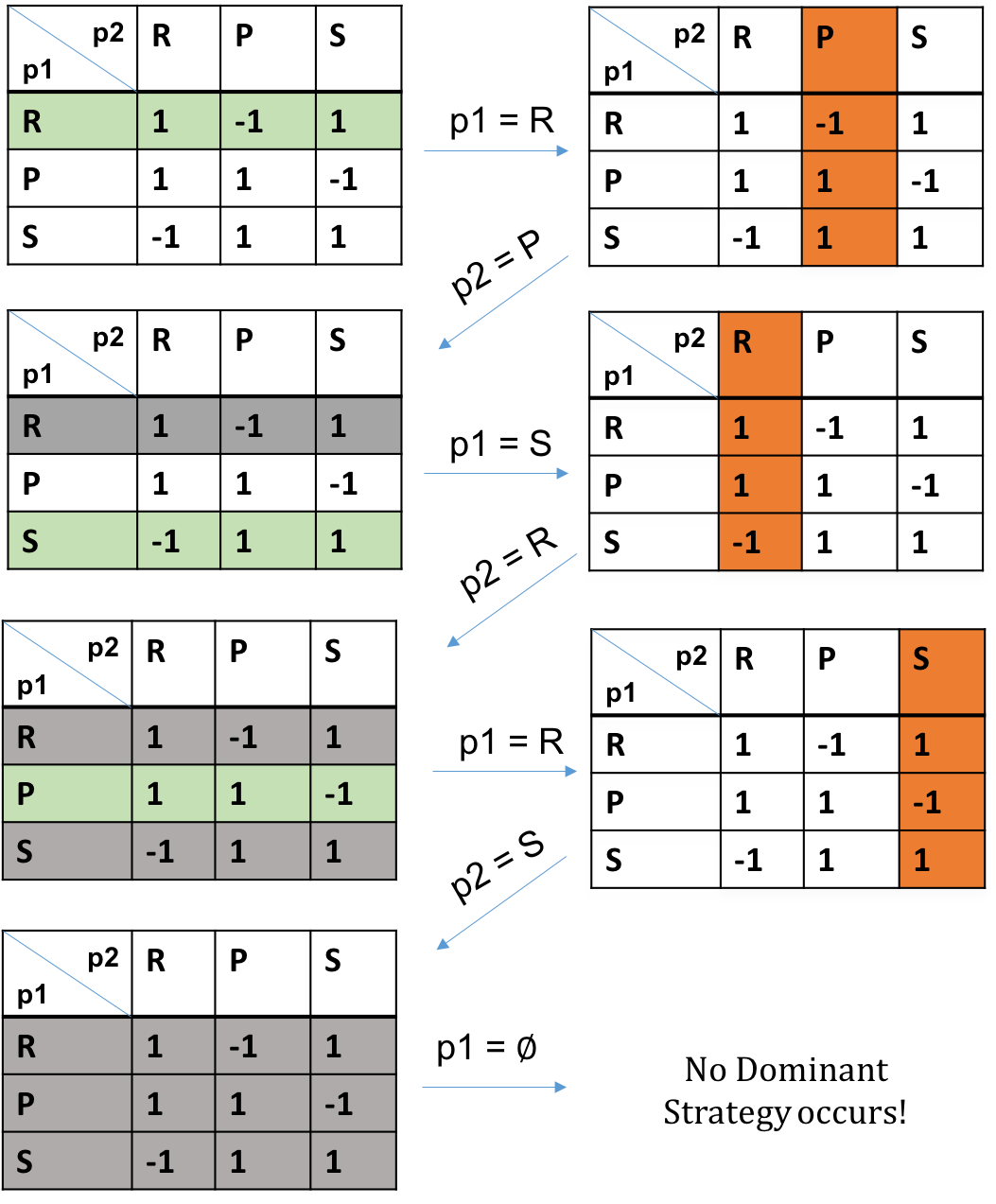
Figure 1: Finding dominant strategies for $p_{1}$

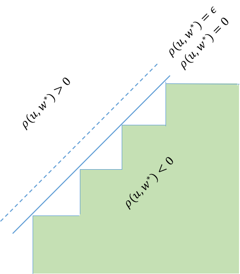
Figure 2: Covering the boundary with rectangles with $\rho=0$ and $\rho=\epsilon>0$.

Continuous Games.  We now turn our attention to games with continuous state spaces. To begin, we will first give an example to illustrate that Alg 1 may not terminate in the continuous setting. This leads to a modification that guarentees termination, given some technical assumptions (Sec 3.1).

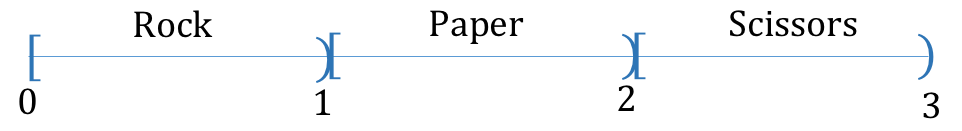
Figure 3: Rock paper scissors as a continuous game

Example 2

We again motivate our construction using the familiar game of rock, paper, scissors (this time embedded into a continuous state space). As before, this game is simple and illustrates the key points. We start by embedding the atomic propositions $R$, $P$, $S$ into $[0,3)$, with $R\mapsto[0,1),P\mapsto[1,2),S\mapsto[2,3)$ (See Fig 3).

Let $i$ and $j$ again denote $p_{1}$ and $p_{2}$’s states resp. Finally, the stateless dynamics of given by:

$$i_{n+1}=u_{n}\wedge j_{n+1}=w_{n}$$ (14)

Where $u(n)\in\mathcal{U},w(n)\in\mathcal{W}$ and $\mathcal{U}=\mathcal{W}=[0,3)$.

As before, we encode $p_{1}$’s objective in Temporal Logic:

$$\begin{split}\varphi_{RPS}&\mathrel{\stackrel{{\scriptstyle\makebox[0.0pt]{\mbox{\tiny def}}}}{{=}}}G_{[0,H]}(\varphi_{s}^{R}\wedge\varphi_{s}^{P}\wedge\varphi_{s}^{S})\\ \varphi_{s}^{R}:&(i\in R)\rightarrow(j\in S)\\ \varphi_{s}^{P}:&(i\in P)\rightarrow(j\in R)\\ \varphi_{s}^{S}:&(i\in S)\rightarrow(j\in P)\end{split}$$ (15)

Where the $(\in)$ operator is simply syntactic sugar. For example the predicate $i\in R$ rewrites to, $i\geq 0\wedge i<1$.

Clearly, applying Alg 1 to find dominant strategies for $p_{1}$ or $p_{2}$ is hopeless since the space of controls, there are infinitely many copies of the $R$, $P$, $S$ moves.

3.1 Adapting CEGIS

Let us reflect on what went wrong during the continuous rock, paper, scissors example. In analogy with the discrete setting, at each round one row (one element of $\mathcal{U}$) of the induced game matrix is refuted. However, because $\mathcal{U}$ now contains infinite elements (and thus infinite rows), termination is not guaranteed. A natural remedy then might be to remove more than just one row at a time. In fact, to make any progress, we would need to remove a non-zero measure subset of $\mathcal{U}$ (or an infinite number of rows).

Remark 3

The CEGIS scheme in [11] uses a maximization oracle to find a counterexample which maximally falsifies the dominant control proposed by the controller. For our purposes we use a satisfaction oracle to find the counterexamples. While the quality of counterexamples may vary (they no longer maximally falsify the control), this does not affect our termination guarantees, though it might affect the rate of convergence. Quantifying this convergence is a topic of future exploration.

Motivated by this reflection, we modify the CEGIS loop to, per iteration, remove all the rows refuted by a given counterexample $\mathbf{w}^{*}$ . A sketch of this algorithm is given in Alg 2.

Algorithm 2 Modified CEGIS scheme

1:procedure ModifedCEGIS($\epsilon$)

2:    Input: $\mathcal{U},\mathcal{W},\phi$

3:    Output: $\mathbf{u}^{*}$

4:    $\mathbf{w}^{*}\sim\mathcal{W}$

5:    while $\mathbf{w}^{*}\neq\bot$ do

6:       $\mathbf{u}^{*}\leftarrow FindSat(\mathbf{w}^{*},\mathcal{U},\phi)$

7:       if $\mathbf{u}^{*}=\bot$ then break        

8:       $\mathbf{w}^{*}\leftarrow FindSat(\mathbf{u}^{*},\mathcal{W},\neg\phi)$

$\star$:       $\mathcal{U}\leftarrow\mathit{WithoutRefuted}_{\epsilon}(\mathbf{w}^{*},\mathcal{U},\phi)$     

10:    return $\mathbf{u}^{*}$

Alg 2 uses a new subroutine, $\mathit{WithoutRefuted}$, which takes the current $\mathbf{w}^{*}$ and removes the refuted region from $\mathcal{U}$. We now make this more precise.

Definition 1

Given $\mathbf{w}^{*}\in\mathcal{W}$ let $\mathcal{U}_{\mathbf{w}^{*}}^{+}$ be the subset of $\mathcal{U}$ s.t. $({\bf u},\mathbf{w}^{*})\models\phi$. Further, let $\mathcal{U}_{\mathbf{w}^{*}}^{-}\mathrel{\stackrel{{\scriptstyle\makebox[0.0pt]{\mbox{\tiny def}}}}{{=}}}\mathcal{U}-\mathcal{U}_{\mathbf{w}^{*}}^{+}$.

Our goal is for $\mathit{WithoutRefuted}$ to remove $\mathcal{U}_{\mathbf{w}^{*}}^{-}$ from $\mathcal{U}$. The key insight of this work is that if the quantitative semantics are Lipschitz Continus in ${\bf u}\in\mathcal{U}$ then a counterexample pair $({\bf u},\mathbf{w}^{*})$ can be generalized to a ball of counterexamples (with radius proportional to degree of satisfaction). Each of these balls has non-zero measure, and thus one expects $\mathcal{U}_{\mathbf{w}^{*}}^{-}$ to be contained in the union of a finite number of these balls.

Generalizing counterexample pairs (${\bf u}$, $\mathbf{w}^{*}$).  Consider a point, ${\bf u}$, in the interior of $\mathcal{U}_{\mathbf{w}^{*}}^{-}$. Since ${\bf u}$ is in $\mathcal{U}_{\mathbf{w}^{*}}^{-}$ and doesn’t lie on the boundary, $\rho^{\phi}({\bf u},\mathbf{w}^{*})<0$. If $L_{u}$ is the Lipschitz bound on the rate of change of $\rho^{\phi}$ w.r.t. changes in ${\bf u}$, then every ${\bf u}^{\prime}$ within the (open) ball of radius $\rho^{\phi}({\bf u},\mathbf{w}^{*})/L_{u}$ of ${\bf u}$ also has robustness less than $0$ and is thus also refuted.

The next example illustrates that $\mathcal{U}_{\mathbf{w}^{*}}^{-}$ is not necessary coverable by a finite number of these balls.

Example 3

Consider the boundary represented by diagonal bold blue line in Fig 2. We see that, approximating the boundary by a finite number of rectangles always leaves out a finite amount of space in $\rho^{\phi}({\bf u},{\bf w}^{*})<0$ which is not covered(shown by the white triangles). Further, the size of rectangle is proportional to size of the robustness. At the boundary this becomes 0, the rectangle induced covers 0 area. To truly approximate the boundary, we would need to compute an infinite number of rectangles, and thus loose our termination guarantees.

Epsilon-Completeness.  Given that we cannot cover $\mathcal{U}_{\mathbf{w}^{*}}^{-}$ exactly, we must ask ourselves what compromises we are willing to accept for termination. Fundamentally, we prefer to err on the side of “safety”, implying over-approximating $\mathcal{U}_{\mathbf{w}^{*}}^{-}$; however we would like to make this over-approximation tunable. This is further motivated by the observation that it is (often) undesirable to have a controller that just barely meets the specification, as due to modeling errors or uncertainty, the system may not perform exactly as expected. As such, one typically seeks “robust” controllers. This leads us to the following proposition: what is the minimum robustness controller we are willing to miss by over-approximating $\mathcal{U}_{\mathbf{w}^{*}}^{-}$?

Algorithm 3 Removes over-approximation of refuted inputs

1:procedure WithoutRefuted($\epsilon$)

2:    Input: ${\bf w},\mathcal{U},\phi$

3:    Output: $\mathcal{U}$

4:    while True do

5:       ${\bf u}\leftarrow FindSat({\bf w},\mathcal{U},\neg\phi)$

6:       if ${\bf u}=\bot$ then break        

7:       $R\leftarrow\epsilon+|\rho^{\phi}({\bf u},{\bf w})|/L_{u}$

8:       $\mathcal{U}\leftarrow\mathcal{U}\setminus\{{\bf u}^{\prime}\in\mathcal{U}\ :\ |{\bf u}-{\bf u}^{\prime}|<R\}$     

9:    return $\mathcal{U}$

Given this concession, we now provide an implementation of $WithoutRefuted$ in Alg 3. For analysis we introduce notation for $\epsilon$-refuted space.

Definition 2

Denote by $\mathcal{U}_{\mathbf{w}^{*}}^{\leq\epsilon}$ the set of inputs that are not $\epsilon$-robust to $\mathbf{w}^{*}$. That is

$$\mathcal{U}_{\mathbf{w}^{*}}^{\leq\epsilon}\mathrel{\stackrel{{\scriptstyle\makebox[0.0pt]{\mbox{\tiny def}}}}{{=}}}\{\forall{\bf u}\in\mathcal{U}_{\mathbf{w}^{*}}^{-}\ :\ \rho({\bf u},{\bf w},\phi)\leq\epsilon\}$$ (16)

Next, we show that Alg 3 over-approximates $\mathcal{U}_{\mathbf{w}^{*}}^{-}$ and under approximates $\mathcal{U}_{\mathbf{w}^{*}}^{\leq\epsilon}$ in a finite number of iterations. As such, this implies line 8 of Alg 3 throws away all of $\mathcal{U}_{\mathbf{w}^{*}}^{-}$, but no controllers that are $\epsilon$-robust.

Lemma 1

Alg 3 always terminates.

Proof 3.1.

Note that the radius of a counterexample ball is atleast $R_{min}\mathrel{\stackrel{{\scriptstyle\makebox[0.0pt]{\mbox{\tiny def}}}}{{=}}}\frac{\epsilon}{L}>0$. Thus, if Alg 3 never terminates, one could find always find a point $R_{min}$ away from all previously sampled points. However, this implies $\mathcal{U}$ is unbounded, which contradicts our assumptions. Thus $\mathit{WithoutRefuted}$ terminates in a finite number of iterations.

Lemma 3.2.

Let $B$ be the result of Alg 3 on $\mathcal{U},\mathbf{w}^{*},{\bf u},\phi$. Then:

$$\mathcal{U}_{\mathbf{w}^{*}}^{-}\subset\mathcal{U}\setminus B\subset\mathcal{U}_{\mathbf{w}^{*}}^{\leq\epsilon}$$ (17)

Proof 3.3.

We must show that $B$ removes from $\mathcal{U}$ only inputs with robustness strictly less than $\epsilon$, i.e. $\mathcal{U}\setminus B\subset\mathcal{U}_{\mathbf{w}^{*}}^{\leq\epsilon}$. Assume for a contradiction that ${\bf u}^{\prime}$ with $\rho^{\phi}({\bf u}^{\prime},{\bf w})\geq\epsilon$ was removed, then there must have been ${\bf u}$ with $|{\bf u}-{\bf u}^{\prime}|<(\epsilon+|\rho^{\phi}({\bf u},{\bf w})|)/L_{u}$, but $\rho^{\phi}({\bf u},{\bf w})\leq 0$. This contradicts the Lipschitz assumption on $\rho$, since we have $|\rho^{\phi}({\bf u}^{\prime},{\bf w})-\rho^{\phi}({\bf u},{\bf w})|\geq\epsilon+|\rho^{\phi}({\bf u},{\bf w})|>L_{u}*|{\bf u}-{\bf u}^{\prime}|$.

Next, let us show the $\mathcal{U}_{\mathbf{w}^{*}}^{-}\subset\mathcal{U}\setminus B$. The termination condition for Alg 3 is that no ${\bf u}$ satisfies $\neg\phi$, so $B$ does not intersect $\mathcal{U}_{\mathbf{w}^{*}}^{-}$. Thus, by construction, we only terminate if $\mathcal{U}_{\mathbf{w}^{*}}^{-}\subset\mathcal{U}\setminus B$.

Remark 3.4.

Note that in order for this set of balls to remain within the theory of Real Linear Arithmetic(RLA), one must use the infinity norm, which has the effect of inducing hyper-square, encodable using $2\cdot n_{u}$ constraints. Explicitly we encode the square centered on $\mathbf{u}^{*}$ as:

$$\left(\bigwedge_{i=1}^{n_{u}}{\bf u}_{i}-\mathbf{u}^{*}_{i}\leq R\right)\wedge\left(\bigwedge_{i=1}^{n_{u}}\mathbf{u}^{*}_{i}-{\bf u}_{i}\leq R\right)$$ (18)

which is a valid formula in RLA.

We are finally ready to state and prove our main theorem regarding the termination of Alg 2.

Theorem 3.5.

For a system which is Lipschitz continuous in control $u$ and disturbance(adversary control) $w$, Alg 2 converges in finite number of iterations for any $\epsilon>0$.

Proof 3.6.

At each iteration, of Alg 2, we are given a $\mathbf{w}^{*}$ and remove an epsilon over-approximation of the $\mathcal{U}_{\mathbf{w}^{*}}^{-}$ (shown in Lemma 3.2). Lemma 1 guarantees that this will halt in finite time. Next, a $\mathbf{u}^{*}$ is computed with maximum robustness w.r.t $\mathbf{w}^{*}$. If no satisfying assignment is found, the loop terminates (and thus terminates in a finite number of iterations). If the a satisfying assignment is found, then because $\mathbf{u}^{*}$ was not thrown out during the over-approximation of $\mathcal{U}_{\mathbf{w}^{*}}^{-}$, $\mathbf{u}^{*}$ must have robustness greater than or equal to $\epsilon$. Thus, to refute $\mathbf{u}^{*}$, the next $\mathbf{w}^{*}$ must, by the Lipschitz bound (as in the proof of Lemma 3.2) be a minimum distance $R_{min}=\frac{\epsilon}{L_{w}}$ away from the previous ${\bf w}$. Thus, as in Lemma 3.2, at each iteration we require $\mathbf{w}^{*}$ to be $R_{min}$ away from all previous counter examples. We have assumed $\mathcal{W}$ to be bounded, thus we only explore a finite number of counter examples, terminating in a finite number of iterations.

Next, we turn to the complexity of Alg 2.

Theorem 3.7.

Alg 2 calls the FindSat Oracle at most

$$O\left(\prod_{i}^{n_{u}}\frac{L_{w}^{H}}{\epsilon^{H}}|\mathcal{W}_{i}|^{H}+\prod_{i}^{n_{w}}\frac{L_{w}^{H}}{\epsilon^{H}}|\mathcal{U}_{i}|^{H}\right)$$

Proof 3.8.

Recall that the termination of Alg 2 and Alg 3 rests on the following question: Is the maximum number points one can place in $\mathcal{U}$ (and $\mathcal{W}$) s.t. they are all $R_{min}$ apart. We now show explicitly the maximum number of samples (and thus Oracle calls). Consider first $\mathcal{U}$, letting $|\mathcal{U}|_{i}$ denote the length of $\mathcal{U}$ in the $i$th dimension (recall that $\mathcal{U}$ is bounded and embedded in $\mathbb{R}^{n_{u}}$). Observe that under the infinity norm, each point induces an $n_{u}$-dimensional square, $S$, of edge length $2R_{min}$ that no other point can lie in. Further, observe that along each edge one can pack 3 points $R_{min}$ apart. We can optimally pack a square lattice (with each leg of the lattice having length $R_{min}$) with $3^{n_{u}}$ points into $S$. W.L.O.G assume that $|\mathcal{U}_{i}|$ is a multiple of $R_{min}$. As squares lattices tessellate, $\mathcal{U}$ can be packed by introducing a $3^{d}$ lattice around each point in our original lattice. Since each point forms a locally optimal packing and because the space is entirely filled this is an optimal packing. Along each lattice row of length $l$ there are $l/R_{min}-1$ points. Taking the product over each axis (including all $H$ copies due to time) yields $\prod_{i}^{n_{w}}\frac{L_{w}^{H}}{\epsilon^{H}}|\mathcal{U}_{i}|^{H}$ points. A similar argument can be made for $\mathcal{W}$. Thus, both the system and environment will run out of choices in

$$O\left(\prod_{i}^{n_{u}}\frac{L_{w}^{H}}{\epsilon^{H}}|\mathcal{W}_{i}|^{H}+\prod_{i}^{n_{w}}\frac{L_{w}^{H}}{\epsilon^{H}}|\mathcal{U}_{i}|^{H}\right)$$

FindSat calls.

Theorem 3.9 (Soundness).

If Alg 2 returns a $\mathbf{u}^{*}\neq\bot$, then $\mathbf{u}^{*}$ is dominant.

Proof 3.10.

Follows directly from Lem 3.2.

Theorem 3.11 ($\epsilon$-Completeness).

If $\mathcal{U}\setminus\mathcal{U}_{\mathbf{w}^{*}}^{\leq\epsilon}\neq\emptyset$ then Alg 2 will return $\mathbf{u}^{*}\in\mathcal{U}_{\mathbf{w}^{*}}^{+}$.

Proof 3.12.

Follows directly from Lem 3.2 and Thm 3.5

Lipschitz Bounds for Linear Dynamics and STL Predicates.  In the previous section, we required computing Lipschitz bounds of $\rho^{\phi}$ w.r.t changes in ${\bf u}$ and ${\bf w}$ in order to guarantee termination. We now show how to automatically compute these bounds for linear systems of the form

$$x_{n+1}=Ax_{n}+Bu_{n}+Cw_{n}$$ (19)

subject to the STL specification $\varphi$ with $\mu(x)=Dx>0$ for some matrix $D$.

We start by observing that if $\rho^{\phi}(x)$ is Lipschitz-bounded in $x$ by $L_{x}$ and $x({\bf u},{\bf w})$ is Lipschitz-bounded in ${\bf u}$ by $L_{u}$, then $\rho^{\phi}$ is Lipschitz bounded in ${\bf u}$ by $L_{u}\cdot L_{x}$.

To compute $L_{x}$, we begin by unrolling the states over a horizon $H$:

$$x_{H}=Ax_{0}+\sum_{i=0}^{H-1}A^{H-1-i}Bu^{i}+\sum_{i=0}^{H-1}A^{H-1-i}Cw^{i}$$ (20)

Differentiating w.r.t. ${\bf u}$ yields:

$$\nabla_{\bf u}x_{H}=\text{diag}(B,AB,A^{2}B,\dots,A^{H-1}B)$$

Letting $\sigma(P)$ be the set of singular values of $P$, a valid Lipschitz bound is then:

$$L_{x}=\max_{s\in\sigma(\nabla_{{\bf u}}x_{H})}(|s|)$$ (21)

The case for $L_{u}$ is similar. Observe that the rate of change in $\rho^{\phi}$ depends only on which $\mu(x)$ the nested $\sup$ or $\inf$ in (7) selects. Thus, we can upper bound $L_{u}$ by taking the maximum rate of change across predicates. If $\mu(x)$ is linear (as we assume in this work), then its rate of change is again upper bounded by its singular values. Thus

$$L_{u}=\max_{\mu}(\max_{s\in\sigma(\mu)}(|s|))$$ (22)

A similar argument over $L_{w}$ gives the Lipschitz bound of $\rho^{\phi}$ w.r.t. ${\bf w}$ .

Example 3.13 (Continuous RPS).

We can represent the continuous RPS in Eqn 14 as a linear system with a combined state space, $x=[i\ j]^{T}$, as,

$$\begin{split}x_{n+1}=\left[\begin{matrix}1&0\\ 0&0\end{matrix}\right]u_{n}+\left[\begin{matrix}0&0\\ 0&1\end{matrix}\right]w_{n}\end{split}$$ (23)

and each atomic predicate is affine with the form

$$\begin{split}\mu(x)=\left[\begin{matrix}1&0\\ 0&1\end{matrix}\right]x-\alpha\end{split}$$ (24)

Analysis of the singular values gives us, $\frac{\partial x}{\partial u}\leq 1$ and $\frac{\partial\rho^{\varphi}}{\partial x}\leq 1$ and thus $\frac{\partial\rho^{\varphi}}{\partial u}\leq 1$. We can thus use the Lipschitz bound $L_{u}=1$. In Fig 4 we throw away squares of length $\rho^{\phi}({\bf u}^{*},{\bf w}^{*})+\epsilon$ for every counterexample ${\bf w}^{*}$ we find for the current dominant strategy ${\bf u}^{*}$. Alg 2 returns ${\bf u}^{*}=\bot$ and we conclude that there is no dominant strategy for the continuous RPS.

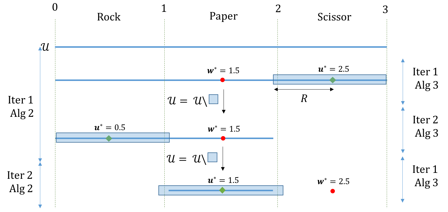
Figure 4: Illustration of Alg 2 in Ex 3.13

Remark 3.14.

Notes on Optimizations and Performance.  To be faithful to the original implementation of the memoryless oracle presented in [11] we need to replace the FindSat oracle with an Optimization oracle. This means that each counterexample is maximally refuting (implying larger magnitude of $\rho$ and therefore quicker convergence in terms of number of oracle calls), but the oracle calls themselves may be much slower. These kinds of trade-offs make it difficult to directly justify one or the other, and thus for ease of exposition, we have only presented a simple satisfaction oracle.

One can imagine modifying the counterexample generalization in many ways. One easy modification is take the counterexample square with radius $R_{min}$ and try to make it larger. To do so, one can binary search for the largest radius, such that all inputs are refuted. By fixing $R$ each of these queries is a single oracle call. Note however, this results in a logarithmic blowup to oracles calls.

We see this technique as being orthogonal and complementary to other conflict analysis techniques. Additional performance gains are to be found in, e,g,, syntactic analysis of $\varphi$ to find more problem specific conflict lemmas.

Before ending this section, we note that one can make the following transformation: $\forall{\bf w}\exists{\bf u}\ .\ ({\bf u},{\bf w})\models\phi\mapsto\neg(\exists{\bf w}\forall{\bf u}\ .\ ({\bf u},{\bf w})\models\neg\phi)$ to handle pure response games, used to test the existence reactive strategies. In such cases, we need to under approximate the subset of $\mathcal{W}$ that ${\bf u}$ is robust to. This is taken care of automatically, by overapproximating $\neg\phi$.

4 Reactive Hierarchy

Failing to find a dominant strategy for $p_{1}$, one may reasonably wonder if if there exists a winning reactive strategy of the form:

$$\exists i_{1}\forall j_{1}\exists i_{2}\forall j_{2}\ .\ (\bf{i},\bf{j})\models\varphi_{RPS}$$ (25)

One technique for searching for such a controller (particularly over arbitrary horizons) is Receding Horizon Control.

Receding Horizon Controller.  Model Predictive Control (MPC) or Receding Horizon Control (RHC) is a well studied method for controller synthesis of dynamical systems [9, 6]. In receding horizon control, at any given time step, the state of the system is observed and and the system plans a controller for next a Horizon $H$. The first step of the controller is then applied, the environment response is observed, and the system replanes for the next $H$ steps. This, allows the system to react to what steps the environment actually performs. MPC has been extended for satisfying $G(\phi)$, where $\phi$ is a bounded Signal Temporal Logic formula with scope $H$ [12]. At each step, one searches for a dominant controller (as in the previous section) and applies the first step. One of the key contributions of [12] is that, one needs to be careful that future actions are consistent with previous choices. A reframing of the observation in  [12] suggests that is sufficient to simply satisfy ${\bf G}({\bf G}_{[-H,H]}(\phi))$. This new specification asserts that $\phi$ holds for the next $H$ steps, and all choices we make are consistent with the previous time steps. Thus, no additional machinery is required.

That said, despite all of its benefits (tractability, well developed theory, reactivity), Receding Horizon Control using dominant controllers may not always be feasible. Further, it provides no mechanism to find a certificate that this strategy truly satisifies $G(\phi)$.

In this work, we attempt to take a step towards this certificate by noticing that the Lipschitz bounds imply nearby strategies produce similar results. This means we can extract decision trees. A certificate that a furture work may then be able to provide is a scheme by which the decision tree returns to a previous state (resulting in a lasso). Motivated by such applications, we explore how to extract reactive controllers for a bounded horizon.

To facilitate development, let us return to our toy example, Rock, Paper, Scissors.

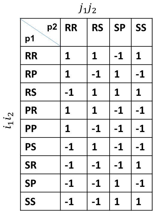
(a) Dominant strategy for $p1$ and $p2$

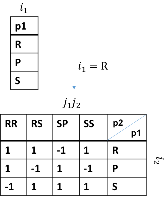
(b) Existence of reactive strategy for $p1$

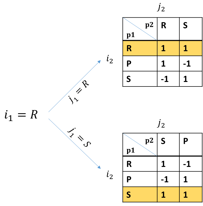
(c) Reactive strategy for $p1$

Figure 5: Rock Paper Scissors rules with assumptions on $p_{2}$

Example 4.15.

Reactive Rock, Paper, Scissors.  Let us slightlt alter our discrete Rock, Paper, Scissors example by constraining the $p_{2}$’s dynamics.

$$\begin{split}&\phi_{j}^{R}:\ {\bf G}\bigg{(}j=R\implies{\bf X}(j=\{R,S\})\bigg{)}\\ &\phi_{j}^{P}:\ {\bf G}\bigg{(}j=P\implies{\bf X}(j=\{P,R\})\bigg{)}\\ &\phi_{j}^{S}:\ {\bf G}\bigg{(}j=S\implies{\bf X}(j=\{S,P\})\bigg{)}\\ &\phi_{j}^{init}:\ j=\{R,S\}\end{split}$$ (26)

$\phi_{j}^{R},\phi_{j}^{P},\phi_{j}^{S}$ enforces the moves $p_{2}$ can make at consecutive time steps and $\phi_{j}^{init}$ is the initial play of $p_{2}$. The overall assumption, $\phi_{RPS}^{a}=\phi_{j}^{R}\wedge\phi_{j}^{P}\wedge\phi_{j}^{S}\wedge\phi_{j}^{init}$.

The specification is given as:

$$\phi=\phi_{RPS}^{a}\rightarrow\phi_{RPS}$$ (27)

Let us assume we play for two turns and follow a similar procedure as last time. A quick scan of Fig 5(a) shows that there’s no all 1’s row. Thus, there is no dominant strategy. Similarly, because there’s no all -1 row, there’s no dominant strategy for the environment. Thus, one has hope in exploring for a reactive strategy.

To do so, we first ask the question: Does there exist a first move $i_{1}$ such that if $p_{2}$ then reveals both $j_{1}$ and $j_{2}$, $p_{1}$ could find a $i_{2}$ that satisfies the specification. Formally:

$$\exists i_{1}\forall j_{1},j_{2}\exists i_{2}\ .\ (\bf{i},\bf{j})\models\varphi_{RPS}$$ (28)

The motivation for first solving eq 28, is that compared to the fully reactive game, it has less quantifier alternations and is thus expected to be “easier”. Moreover, this query lets one eliminate $i_{1}$ choices that even with future knowledge of $j_{2}$ couldn’t win. As we can see in Fig 5(b), if $i_{1}=R$, then $j_{2}$ has no winning strategy. Proceeding in a Depth First Search fashion, we see if $i_{1}=R$, $\forall j_{1}\exists i_{2}\forall j_{2}\ .\ (\bf{i},\bf{j})\models\phi$. Fig 5(b) shows that if $i_{1}=R$, then if $j_{1}=R$, $i_{2}$ should be $R$. Similarly, if $j_{2}=S$ then $i_{2}$ should be $S$. Or simply, $i_{2}(j_{1})=j_{1}$. Thus, eq 25 is satisfied.Fig 5(c) shows the computed strategy.

Remark 4.16.

While in the discrete setting, when $|\mathcal{U}|$ is small, doing the queries in this order may not save much effort. However, if $|\mathcal{U}|$ is very large (or even infinite), then pruning the $\mathcal{U}$ using easier queries, has huge benefits.

We now turn to systematizing the technique we applied in the example. Recall that a dominant strategy takes the form:

$$\exists{\bf u}^{H}\forall{\bf w}^{H}\ .\ ({\bf u}^{H},{\bf w}^{H})\models\phi$$ (29)

where, ${\bf u}^{H}$ and ${\bf w}^{H}$ are, respectively, the system ($p_{1}$) control and environment ($p_{2}$) disturbance over a horizon $H$.

Note that this quantification means that the controller is not aware in advance of the disturbance over the time horizon $H$. As such, the controller is at a complete disadvantage while planning its actions. Adding a reaction by allowing a quantifier alternation gives the system more information allowing for more winning strategies. We show the hierarchy of games (ordered by the number of winning controllers) in Fig 6.

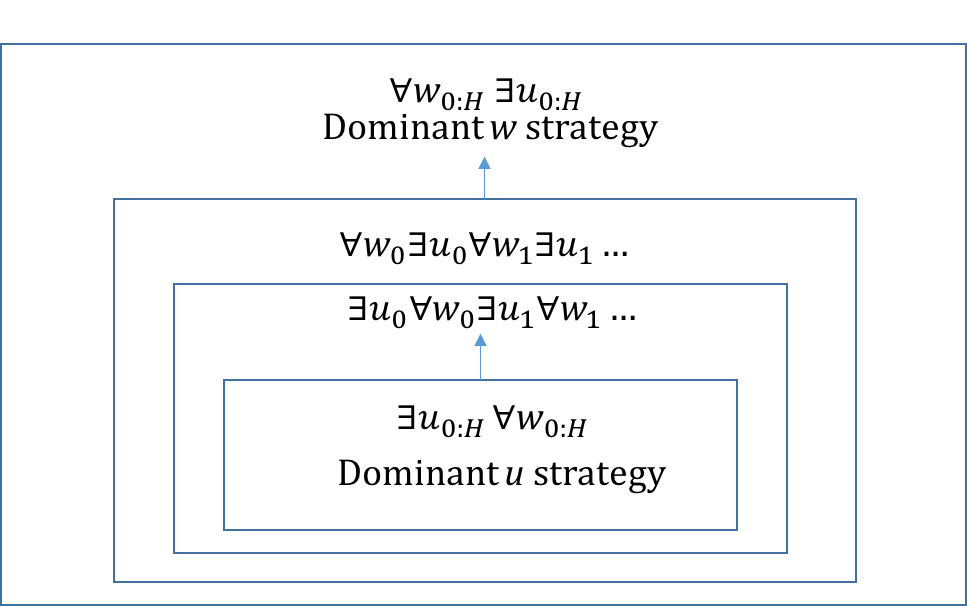
Figure 6: Control strategies for different games

Note however that only certain games yield controllers which are implementable in our setting. As the players reveal their solutions simultaneously, $u_{k}$ can only depend on plays (by both the system and the environment) before round $k$. We call these games the “causal” set and will define them more precisely in a moment. If each input depends on all previous moves, we call this a fully reactive controller, and in general these controllers solve:

$$\exists\mathbf{u}_{0}\forall\mathbf{w}_{0}\exists\mathbf{u}_{1}\forall\mathbf{w}_{1}\dots\exists\mathbf{u}_{H-1}\forall\mathbf{w}_{H-1}\ .\ ({\bf u}^{H},{\bf w}^{H})\models\phi$$ (30)

If a solution to Eqn 30 does not exist, then there exists no control when the system plays first.

Remark 4.17.

There may still be a control if the environment plays first. This is a simple extension of the work presented, but it handling such cases complicates exposition.

Now let us define the set of games under consideration:

Definition 4.18 (Order Preserving Games).

Consider the alphabet:

$$\Sigma\mathrel{\stackrel{{\scriptstyle\makebox[0.0pt]{\mbox{\tiny def}}}}{{=}}}\{\exists u_{1},\exists u_{2},\dots,\exists u_{H},\forall w_{1},\forall w_{2},\dots,\forall w_{H}\}$$

• Let $\sigma_{u}$ denote the string $\exists u_{0}\exists u_{1}\dots\exists u_{H-1}$

• Let $\sigma_{w}$ denote the string $\forall w_{0}\forall w_{1}\dots\forall w_{H-1}$.

We define the set of Order Preserving Games $Q$ as all possible interleavings of $\sigma_{u}$ and $\sigma_{w}$.

This set is called order preserving, since by construction the elements of $\sigma_{u}$ and $\sigma_{w}$ are ordered temporally, and thus their interleavings preserve the order. Evaluation of such a game is denoted by:

Definition 4.19.

Given $q\in Q$

$$\llbracket q\rrbracket\mathrel{\stackrel{{\scriptstyle\makebox[0.0pt]{\mbox{\tiny def}}}}{{=}}}q\in Q,\ q\ .\ ({\bf u}^{H},{\bf w}^{H})\models\phi$$ (31)

Next, we define the previously mentioned causal games:

Definition 4.20.

The causal subset of $Q$ is defined by:

$$A\mathrel{\stackrel{{\scriptstyle\makebox[0.0pt]{\mbox{\tiny def}}}}{{=}}}\{q:q\in Q\wedge\text{pos}(q,u_{k})<\text{pos}(q,w_{k})\}$$ (32)

where $\text{pos}(q,a)$ gives the position of $a$ in string $q$.

Finally, it’s useful to define two string operations: $extend(q,k)$ and $reveal(q,k)$ defined as follows: $extend(q,k)$ moves $\exists u_{k+1}$ immediately after $\exists u_{k}$ in $q$. $reveal(q,k)$ moves all environment moves up to round $k-1$ that appear after $\exists u_{k}$ in $q$ immediately before $\exists u_{k}$.

Game Transition System. We now construct a Labeled Transition System, $\mathcal{D}$, specified by a tuple of (nodes, edges, labels, initial state)

$$\mathcal{D}=(\sigma_{u}\times(Q\cup\{\bot,\mathbb{C})\},E,\{False,True\},a_{0})$$ (33)

that formalizes the progression of games seen in the Rock, Paper, Scissors example. $Q$ is again the set of games, $\{\bot,\mathbb{C}\}$ are sink nodes representing no causal control does not exists and does exists resp. $\sigma_{u}\times Q$ represents the set of decision variable and games combinations. $a_{0}$ is tuple of the easiest non-dominant game where $p_{1}$ plays first and the first (temporal) decision.

$$a_{0}=(\exists u_{1},\exists u_{1}\forall{\bf w}^{H}\exists u_{2}\ldots u_{H})$$ (34)

and the edges, $E$, are defines as follows:

Definition 4.21.

An edge, $e\in E$, is a tuple

$$((\exists u_{k},q),(\exists u_{j},q^{\prime}),L)$$

An edge, $e$ is in $E$ iff one of the following is True:

$$L\wedge q_{1}\in A\wedge q_{2}=\mathbb{C}$$ (35)

$$\neg L\wedge\text{pos}(q_{1},{\bf w}_{k})=\text{pos}(q_{1},u_{k})-1\wedge q_{2}=\bot$$ (36)

$$L\wedge q\notin A\wedge q_{2}=extend(q_{1},k)\wedge j=k+1$$ (37)

$$\begin{split}&\neg L\wedge\text{pos}(q_{1},{\bf w}_{k})>\text{pos}(q_{1},u_{k})\\ &\wedge q_{2}=reveal(q_{1},k)\wedge j=k\end{split}$$ (38)

Informally, movement through $\mathcal{D}$ is as follows: We first compute $\llbracket q\rrbracket$. If it evaluates to True, we either have a causal controller, or we try to avoid adding an extra quantifier by extending the dominant fragment. If $\llbracket q\rrbracket$ evaluates to False, then we allow $u_{k}$ to depend on moves the environment has played since the last dominant fragment. If there aren’t any, we move to bottom, since this implies we must see the environments next move to proceed with this prefix of a decision tree. We show $\mathcal{D}$ for $H=3$ in Fig 7.

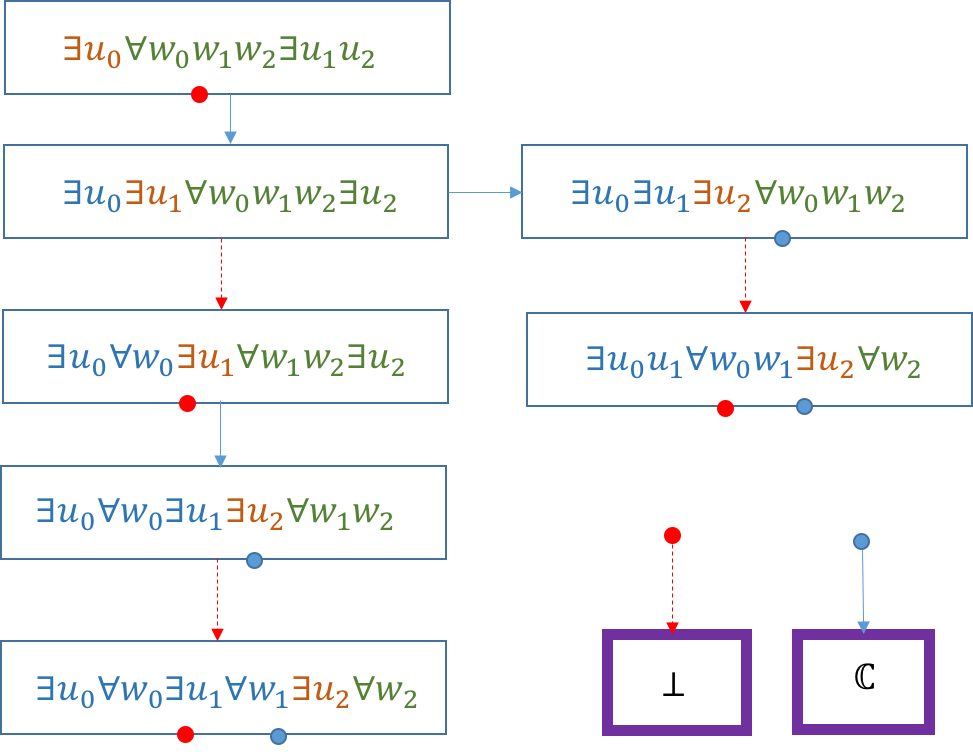
Figure 7: Game graph for $H$ = 3. The orange substring is the decision variable. Red marks False Edge. Blue marks True Edge.

Now let us show that moving through our transition system takes at most $2H$ steps. We start by defining a measure:

Definition 4.22 ($\alpha$).

Let $u_{k}$, $q$ be the decision variable and game of node $a$. Pattern matching $q=p\exists u_{k}s$, we define $\alpha(a)$ to be the number of characters of $\sigma_{u}$ that appear in the string $\exists u_{k}s$.

For $q=\exists u_{1}s$, we thus have $\alpha(q)=H-1$.

For $q=\bot$ or $q=\mathbb{C}$, we define $\alpha(a)=0$.

Next we show that our measure is non-increasing.

Lemma 4.23.

$\alpha$ is non-increasing on any path rooted on $q_{0}$

Proof 4.24.

It suffices to show that $\alpha$ is non-decreasing along all edges of $\mathcal{D}$. While traversing Edge (37), the decision variable changes from $\exists u_{k}$ to $\exists u_{k+1}$, and hence $\alpha$ decreases by 1. While traversing Edge (38), the decision variable remains the same (since only variables that have already been played are moved before the current decision variable) , and hence $\alpha$ remains the same. Traversing Edge (36) and Edge (35) directly reduces $\alpha$ to 0. Hence, along any edge $\alpha$ decreases by at most 1.

Next, we show that $\alpha$ doesn’t remain constant for more than 1 transition.

Lemma 4.25.

Any path through $\mathcal{D}$ with two consecutive edge labels False, lead to $\bot$

Proof 4.26.

Aside from Edge (36), the only other type of edge with label false is Edge (38). reveal moves all revealed $w_{j}$ before $u_{k}$, thus the condition for Edge (36) is true and condition for Edge (38) is false.

This leads us to our bound on the number of transitions one does.

Theorem 4.27.

It takes at most $2H$ transitions to traverse from the root node to $\bot$ or $\mathbb{C}$

Proof 4.28.

By Lemmas 4.23 and 4.25 any two transitions either lead to $\bot$ (causing $\alpha$ to go to 0) or contain a True edge. True edges either lead to $\mathbb{C}$ (causing $\alpha$ to go to 0) or decrease $\alpha$ by 1. Thus, every two transitions alpha decreases by at least 1. Thus $\alpha$ becomes 0 after at most $2H$ transitions. Finally, by construction $\alpha=0$ only on $\bot$ or $\mathbb{C}$.

Building a Decision Tree.  We now turn to how to systematically extract a causal decision tree by moving through $\mathcal{D}$. We begin by noting that for each game, $q$ we can associate a decision tree. For a dominant strategy, this corresponds to a chain. For $\forall{\bf w}\exists{\bf u}$ this is a root forking into multiple paths based on ${\bf w}$. The first node, $a_{0}$, of $\mathcal{D}$ corresponds to a single choice $u_{1}$ and then a forking based on ${\bf w}$. As this forking is not causal, we view it as a place holder for a causal subtree to be inserted. We illustrate these trees for a few examples in Figure 8. We’ve annotated “dominant” fragments where the choice is independent of previous $w_{k}$ with blue nodes. The red nodes are nodes that depend on the environment’s choice of $w_{k}$. The pink triangles correspond to a non-causal subtrees. One completes the decision tree by querying if there exists a solution to the next game in $\mathcal{D}$, fixing the path in the decision leading up to a non-causal subtree. Importantly, at every stage, only 1 decision is required and the rest of the prefix can be turned into a call for whether there exists a dominant solution (either for the system of the environment). If so, one replaces the subtree with the new tree. The process repeats until there are no non-causal segments. Reading Figure 8 left to right can be seen as a cartoon of this process.

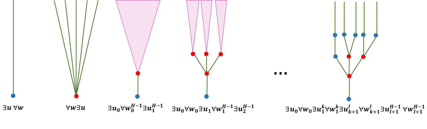
Figure 8: Illustrations of building the decision tree by moving through $\mathcal{D}$.

Again allowing ourselves to miss controllers that are not $\epsilon$ robust, we are able to effectively discretize the space into $R_{min}$ size squares. Thus, one only requires finite branching.

To illustrate this process on a continuous system, we return to our toy example.

Example 4.29.

Recall the Rock, Paper, Scissors example with constrained environment (Ex 4.15). We now modify this example to have the following dynamics:

$$i_{n+1}=i_{n}+u_{n}\ \wedge\ j_{n+1}=j_{n}+w_{n}$$ (39)

where $u_{n}\in[0,1]$ and $w_{n}\in[0,1]$, which are again an instance of Real Linear Arithmetic.

We modify Fig 3 to contain a region of uncertainty of radius, $\delta$, near the boundaries, shown in Fig 9.

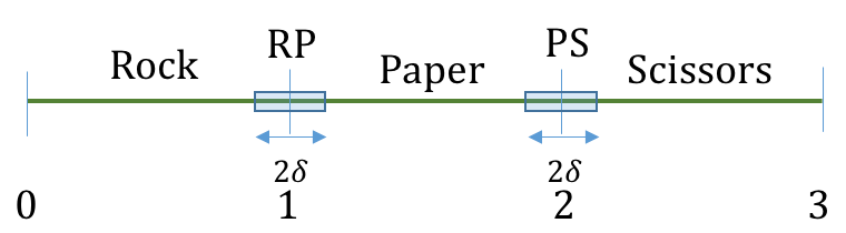
Figure 9: Modified RPS with $\delta$ regions at the boundary

$p_{1}$’s objective is given as $\varphi_{RPS}\mathrel{\stackrel{{\scriptstyle\makebox[0.0pt]{\mbox{\tiny def}}}}{{=}}}\varphi_{d}\wedge\varphi^{m}_{RPS}$, where

$$\begin{split}\varphi^{m}_{RPS}&\mathrel{\stackrel{{\scriptstyle\makebox[0.0pt]{\mbox{\tiny def}}}}{{=}}}G_{[0,H]}(\varphi_{s}^{R}\wedge\varphi_{s}^{P}\wedge\varphi_{s}^{S}\wedge\varphi_{init})\\ \varphi_{s}^{R}:&(i\in R)\rightarrow(j\in\{S,PS\})\\ \varphi_{s}^{P}:&(i\in P)\rightarrow(j\in\{R,RP\})\\ \varphi_{s}^{S}:&(i\in S)\rightarrow(j\in\{P,PS,RP\})\\ \varphi_{init}:&(i=0.5)\wedge(j=0.5)\end{split}$$ (40)

As in Sec 4.15, we consider two turns: $\mathcal{U}=\mathcal{W}=[0,1]^{2}$. For this example $\delta=\epsilon=\frac{1}{8}$.

We first search for a dominant strategy for $p_{1}$ by attempting to find $\exists u_{0}u_{1}\forall w_{0}w_{1}\varphi_{RPS}$. We use Alg 3, to cover $\mathcal{U}$ with squares. Consider $w_{0}w_{1}=00$ i.e., $j_{1},j_{2}=RR$. This would falsify any $u_{0}u_{1}$ such that $i_{2}\in\{S,PS\}$, i.e.,

$$u_{0}+u_{1}+i_{0} \geq 2-\delta\Rightarrow u_{0}+u_{1}\geq 1.5-\delta$$

Now consider $w_{0}w_{1}=11$, i.e., $j_{1}j_{2}=PS$. This would falsify any $u_{0}u_{1}$ such that $i_{1}=\{R,RP\}$ or $i_{2}=\{P,RP,PS\}$, i.e.,

$$u_{0}+i_{0} \leq 1+\delta\Rightarrow u_{0}\leq 0.5+\delta$$

$$u_{0}+u_{1}+i_{0} \leq 2+\delta\Rightarrow u_{0}+u_{1}\leq 1.5+\delta$$

From Fig 10(a) we see the entire $\mathcal{U}$ thrown away. We conclude a dominant $p1$ strategy does not exist.

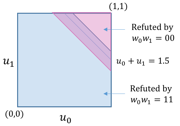
(a) Finding dominant strategy $p1$

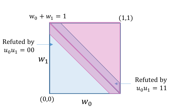
(b) Finding dominant strategy for $p2$

We apply a similar procedure to search for a dominant strategy for $p_{2}$ and see from Fig 10(b) that it does not exist.

Moving to the next game in $\mathcal{D}$, we check we can find a ${\bf u}_{0}$ such that $\exists u_{0}\forall w_{0}w_{1}\exists u_{1}\varphi_{RPS}$ is True. Note that the dynamics are Lipschitz continuous with $u_{n}$ and $w_{n}$ with bound $L=1$. This allows us to break to the $\mathcal{U}$ for $u_{0}\in[0,1]$ in segments of length $\geq\frac{\epsilon}{L}=\frac{1}{8}$. Consider $u_{0}\in[0,\frac{1}{8}]$. Notice, there exists a dominant response $w_{0}w_{1}=1*$, causing the CEGIS query to return false. Discarding $u_{0}=\frac{1}{8}$, we have, $\mathcal{U}=(\frac{1}{8},1]$. Let us now consider $u_{0}\in(\frac{7}{8},1]=1$. Using the Alg 2, we see that there does not exist a dominant $w_{0}w_{1}$. This concludes that a reactive strategy using $u_{0}=1$ exists. Moving on to the final game, $\exists u_{0}\forall w_{0}\exists u_{1}\forall w_{1}\varphi_{RPS}$. Recalling our previous decision $u_{0}=1$, i.e., $i_{1}=P$, we search over $w_{0}$ to solve for $\forall w_{0}\exists u_{1}\forall w_{1}\varphi_{RPS}$. Again, using the Lipschitz bound $L=1$ and $\epsilon=\frac{1}{8}$, we can break the $\mathcal{W}$ for $w_{0}\in[0,1]$ in segments of length $\geq\frac{\epsilon}{L}=\frac{1}{8}$. We now visit each segment of $w_{0}$ and find the dominant $u_{1}$. Let $w_{0}=[0,\frac{1}{8}]$, i.e., $j_{1}\leq\frac{5}{8}\in R$. Since $i=P$ beats $j=R$, $u_{1}=0$ is a dominant play. Since $i_{1}=P$ beats $j_{1}=\{R,RP\}$, we can continue this reasoning for any segments such that $w_{0}\leq\frac{5}{8}$. Let us now consider $w_{0}\in(\frac{5}{8},\frac{6}{8}]$, i.e., $j_{1}=P$. In this case $u_{1}=1$, i.e., $i_{2}=S$ is a dominant play for the system. We now have a decision tree, Fig 10

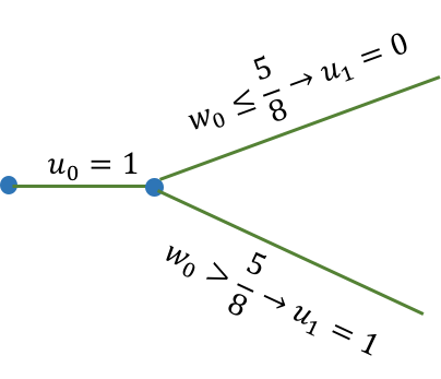
Figure 10: Decision Tree for continuous RPS with dynamics

5 Conclusion

We have presented a methodology to build reactive controllers for Lipschitz continuous systems. We described an efficient tunable CEGIS scheme based on optimization and SMT for synthesizing controllers for Lipschitz continuous systems in an adversarial environment. This algorithm generalizes counterexample pairs and is guaranteed to terminate. We utilized the quantitative semantics of STL to discard regions of our control space to find $\epsilon$ robust strategies. In the absence of a dominant strategy, we find a causal reactive strategy that can be expressed as decision trees. There are a number of directions one could imagine extending this work. A promising direction is to attempt to create lassos from the decision trees, resulting in infinite horizon controllers. Another direction is to incorporate less more intelligent conflict analysis to provide better conflict lemmas. Lastly, a theoretical/empirical understanding of the trade-off between the maximization oracle vs the satisifcation oracle would be immensely valuable.

References

- [1] A. Abate, I. Bessa, D. Cattaruzza, L. Cordeiro, C. David, P. Kesseli, and D. Kroening. Sound and automated synthesis of digital stabilizing controllers for continuous plants. In Proceedings of the 20th International Conference on Hybrid Systems: Computation and Control, HSCC ’17, pages 197–206, New York, NY, USA, 2017. ACM.
- [2] A. Donzé, T. Ferrère, and O. Maler. Efficient robust monitoring for STL. In Computer Aided Verification, 2013.
- [3] A. Donzé and O. Maler. Robust satisfaction of temporal logic over real-valued signals. In International Conference on Formal Modeling and Analysis of Timed Systems, 2010.
- [4] A. Donzé, O. Maler, E. Bartocci, D. Nickovic, R. Grosu, and S. Smolka. On temporal logic and signal processing. In Automated Technology for Verification and Analysis. 2012.
- [5] S. S. Farahani, V. Raman, and R. M. Murray. Robust model predictive control for signal temporal logic synthesis. IFAC-PapersOnLine, 48(27):323–328, 2015.
- [6] C. E. Garcia, D. M. Prett, and M. Morari. Model predictive control: theory and practice–a survey. Automatica, 25, 1989.
- [7] R. Koymans. Specifying real-time properties with metric temporal logic. Real-time systems, 2(4):255–299, 1990.
- [8] O. Maler and D. Nickovic. Monitoring temporal properties of continuous signals. In Formal Techniques, Modelling and Analysis of Timed and Fault-Tolerant Systems. 2004.
- [9] M. Morari, C. Garcia, J. Lee, and D. Prett. Model predictive control. Prentice Hall Englewood Cliffs, NJ, 1993.
- [10] A. Pnueli. The temporal logic of programs. In Proceedings of the 18th Annual Symposium on Foundations of Computer Science, SFCS ’77, pages 46–57, Washington, DC, USA, 1977. IEEE Computer Society.
- [11] V. Raman, A. Donzé, D. Sadigh, R. M. Murray, and S. A. Seshia. Reactive synthesis from signal temporal logic specifications. In Proc. Int. Conf. Hybrid Systems: Computation and Control, 2015.
- [12] V. Raman, M. Maasoumy, A. Donzé, R. M. Murray, A. Sangiovanni-Vincentelli, and S. A. Seshia. Model predictive control with signal temporal logic specifications. In IEEE Conf. on Decision and Control, 2014.
- [13] A. Solar-Lezama, L. Tancau, R. Bodik, S. Seshia, and V. Saraswat. Combinatorial sketching for finite programs. ACM SIGOPS Operating Systems Review, 40(5):404–415, 2006.
- [14] T. Wongpiromsarn, U. Topcu, and R. M. Murray. Receding horizon control for temporal logic specifications. In Proceedings of the 13th ACM international conference on Hybrid systems: computation and control, pages 101–110. ACM, 2010.