Broad Linewidth of Antiferromagnetic Spin Wave due to Electron Correlation

Abstract

We study magnetic excitations in a bilayer of an antiferromagnetic (AF) insulator and a correlated metal, in which double occupancy is forbidden. The effective action of the AF spin wave in the AF insulator is derived by using the path integral formula within the second order of interplane coupling. The electron correlation in the correlated metal is treated by the Gutzwiller approximation, which renormalizes the hopping integrals by $g_{t}$ as proportional to the hole density. The linewidth of the AF spin wave excitations originates from particle-hole excitations in the correlated metal. By increasing the correlation effect, i.e., by decreasing $g_{t}$, it is found that the linewidth at low energies increases inversely proportional to $g_{t}$. The present results will also be useful for bilayers of a metal and ferrimagnet.

I Introduction

A high-$T_{c}$ cuprate shows superconductivity by doping carriers in a Mott insulator, which is an antiferromagnetic (AF) insulator lee ; ogata08 ; keimer . Its magnetic excitation has been observed by inelastic neutron scattering (INS) measurement and is well described by AF spin waves vaknin ; yamada87 ; birgeneau ; hayden ; coldea ; headings . Since a cuprate is magnetically almost isotropic, the AF spin wave is approximately gapless, appearing at the commensurate wavenumber. By doping holes, on the other hand, low-energy magnetic excitations appear at incommensurate wavenumbers yoshizawa ; shirane89 ; yamada , and the overall feature of magnetic excitations changes from the usual AF spin wave to an hourglass-like spectrum tranquada04 ; fujita ; vignolle ; reznik ; lipscombe ; norman ; yamase06 . This variation of magnetic excitations is apparently caused by doped holes. However, some experimental studies using resonant inelastic X-ray scattering letacon and INS matsuura ; sato report that a high-energy part of magnetic excitation is not affected by doped holes. Naively thinking, both low- and high-energy parts could be changed by doping, while the situation is rather close to the low-energy part coming from a Fermi surface, i.e., metallic nature, and the high-energy part having a localized nature. Furthermore, it is also claimed that two components, i.e., commensurate and incommensurate, comprise the magnetic excitations at low energies sato .

The recent development of neutron facilities enables us to observe magnetic excitations more accurately in wider regions of energy and momentum. In addition to the position and intensity of magnetic excitations, the width of peaks is also an important tool to extract relevant interactions of magnons and to elucidate the criticality of magnetism bayrakci ; bayrakci2 ; tseng . In three dimensions, the linewidth of AF spin waves is proportional to $k^{2}$ with wavenumber $k$ harris , which coincides with a prediction by hydrodynamics halperin , while it becomes proportional to $k$ in two dimensions tyc . The former case of proportionality with $k^{2}$ originates from short-wavelength magnon interactions, whereas long-wavelength magnon interactions are relevant to the latter one tyc . For reference, we also consider a ferromagnet. Above the Curie temperature, the linewidth of paramagnons is proportional to $k$. However, near the critical temperature in some materials, e.g., UGe₂ and UCoGe, their linewidth is independent of $k$ chubukov . The constant linewidth in a ferromagnet cannot be satisfied by one type of excitation. Thus, these systems require the presence of both itinerant and localized components chubukov . Although this situation is different from that of cuprates, it implies that the essential nature of magnetic excitations can be clarified by the linewidth of magnetic excitations.

In this paper, we study a bilayer system of an AF insulator and a correlated metal (CM), in which double occupancy is forbidden. The AF spin wave in the AF insulator is calculated and its linewidth is estimated by second-order perturbation theory with respect to an interplane magnetic exchange interaction. The correlation effect is treated by the Gutzwiller approximation. Such a bilayer system is realized in multilayered cuprates having several CuO₂ planes in a unit cell. Due to the different chemical environment between the outer and inner planes, the carrier concentration in the outer plane is different from that in the inner one kondo89 ; stasio90 . In some cases, an alternating stack of superconducting and AF planes is realized, as observed by nuclear magnetic resonance trokiner91 ; mukuda12 , and has been studied theoretically mori02 ; mori05 ; mori06 . Furthermore, a bilayer of a magnet and metal is one of the basic device structures in spintronics. For example, the spin Seebeck effect produces electricity by applying a temperature gradient to a bilayer of a ferromagnet and metal uchida08 ; adachi13 . In such a study, a ferrimagnet is often used as a ferromagnet. However, a ferrimagnet has several particular aspects different from a ferromagnet, e.g., acoustic and optical spin wave excitations, compensation temperature, and so on ohnuma ; kikkawa ; geprags . The linewidth of a spin wave in a ferrimagnet is crucial to improve the efficiency of the spin Seebeck effect. Our results are applicable to ferrimagnetic spin waves.

The rest of the paper is organized as follows. In Sect. II, the Hamiltonian of the bilayer will be given and the effective action of Holstein–Primakoff bosons will be derived by using the path integral formula and the Gutzwiller approximation. In Sect. III, the AF spin wave with the linewidth originating from the CM will be shown numerically. Finally, a summary and discussion will be given in Sect. IV. The appendix on ferrimagnets will be useful from the viewpoint of spintronics.

II Model and Method

We consider the bilayer model of the AF insulator and the CM shown in Fig. 1.

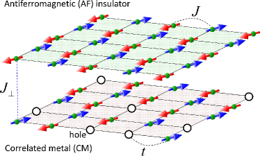
Figure 1: (Color online) Bilayer model of the AF insulator and the CM. The upper plane is the AF insulator and the lower one is the CM, in which double occupancy is forbidden. The arrows indicate localized spins and the white circles indicate doped holes. The magnitudes of in-plane and interplane magnetic exchange interactions are denoted by $J$ and $J_{\perp}$, respectively. In this paper, $J$ in the CM is not considered. The hopping integral of electrons in the CM plane is denoted by $t$ ($t^{\prime}$ and $t^{\prime\prime}$ are not shown in this figure). Note that one-particle hopping is not allowed between planes due to the constraint of no double occupancy mori06 .

The Hamiltonian of the bilayer $H_{\rm BL}$, Eq. (1), is composed of three parts: $H_{\rm AF}$ for the AF insulator, $H_{\rm CM}$ for the CM, and $H_{\rm I}$ for the interplane coupling. The magnetic exchange interaction $J$ in Eq. (2) is imposed on nearest-neighbor spins $\vec{S}_{i}$ and $\vec{S}_{j}$ on sites $i$ and $j$ in the AF plane, respectively. Below, the lattice is divided into sublattices $A$ and $B$, and indices $i$ and $j$ are associated with sublattices $A$ and $B$, respectively, i.e., $i\in A$ and $j\in B$. In Eq. (3), electron creation (annihilation) operators with spin $\sigma$ on sites $i\in A$ and $j\in B$ are denoted by $c_{i,\sigma}^{\dagger}$ ($c_{i,\sigma}$) and $d_{j,\sigma}^{\dagger}$ ($d_{j,\sigma}$), respectively. Each operator has a constraint of no double occupancy on each site. The hopping integrals between first ($t$), second ($t^{\prime}$), and third ($t^{\prime\prime}$) neighboring sites are included, and $i^{\prime}$ ($j^{\prime}$) and $i^{\prime\prime}$ ($j^{\prime\prime}$) denote first- and second-neighbor sites belonging to the same $A$ ($B$) sublattice, respectively. The interplane coupling $J_{\perp}$ in Eq. (4) is a magnetic exchange interaction between the AF and CM planes. Electron hopping is forbidden between these planes since the AF plane does not have holes, and double occupancy is also forbidden mori06 . The spin operator on site $i$ in the CM plane is denoted by $\vec{\sigma}_{i}$.

$$H_{\rm BL} = {H_{\rm AF}}+{H_{\rm CM}}+{H_{\rm I}}$$ (1)

$${H_{\rm AF}} = J\sum\limits_{\left\langle{i,j}\right\rangle}{{{\vec{S}}_{i}}\cdot{{\vec{S}}_{j}}}$$ (2)

$${H_{\rm CM}} = -t\sum_{\left\langle i,j\right\rangle,\sigma}\left(c_{i\sigma}^{\dagger}d_{j\sigma}+h.c.\right)$$ (3)

$$+ t^{\prime}\sum_{\left\langle i,i^{\prime}\right\rangle,\sigma}\left(c_{i\sigma}^{\dagger}c_{i^{\prime}\sigma}+h.c.\right)-t^{\prime\prime}\sum_{\left\langle i,i^{\prime\prime}\right\rangle,\sigma}\left(c_{i\sigma}^{\dagger}c_{i^{\prime\prime}\sigma}+h.c.\right)$$

$$+ t^{\prime}\sum_{\left\langle j,j^{\prime}\right\rangle,\sigma}\left(d_{j\sigma}^{\dagger}d_{j^{\prime}\sigma}+h.c.\right)-t^{\prime\prime}\sum_{\left\langle j,j^{\prime\prime}\right\rangle,\sigma}\left(d_{j\sigma}^{\dagger}d_{j^{\prime\prime}\sigma}+h.c.\right)$$

$$+ {J_{\bot}}S\left({\sum\limits_{i}{\sigma_{i}^{z}}-\sum\limits_{j}{\sigma_{j}^{z}}}\right),$$

$${H_{\rm I}} = {J_{\bot}}\sum\limits_{i}{{{\vec{S}}_{i}}}\cdot{{\vec{\sigma}}_{i}}.$$ (4)

Here, $t$=2.5, $t^{\prime}$=0.85, $t^{\prime\prime}$=0.58, $J$=1, and $J_{\perp}$=0.1.

The Holstein–Primakoff bosons $a_{i}^{\dagger},a_{i}$ on sublattice $A$ and $b_{j}^{\dagger},b_{j}$ on sublattice $B$ are defined by $S_{i}^{-}=\sqrt{2S}a_{i}^{\dagger}\left(1-a_{i}^{\dagger}a_{i}/(2S)\right)^{1/2}$, $S_{i}^{+}=\sqrt{2S}\left(1-a_{i}^{\dagger}a_{i}/(2S)\right)^{1/2}a_{i}$, $S_{i}^{z}=S-a_{i}^{\dagger}{a_{i}}$, $S_{j}^{+}=\sqrt{2S}b_{j}^{\dagger}\left(1-b_{j}^{\dagger}b_{j}/(2S)\right)^{1/2}$, $S_{j}^{-}=\sqrt{2S}\left(1-b_{j}^{\dagger}b_{j}/(2S)\right)^{1/2}b_{j}$, $S_{j}^{z}=b_{j}^{\dagger}{b_{j}}-S$, and $S$=1/2. Up to the first order of the Holstein–Primakoff bosons around the Néel order, the Hamiltonian in Eq. (1) is transformed as

$${H_{\rm HP}} = {H_{\rm sw}}+{H_{\rm e}}+{H_{\perp}},$$ (5)

$${H_{\rm sw}} = JS\sum\limits_{i,\eta}{\left({{{a_{i}}{b_{j}}+a_{i}^{\dagger}b_{j}^{\dagger}}+a_{i}^{\dagger}{a_{i}}+b_{j}^{\dagger}{b_{j}}}\right)},$$ (6)

$$H_{\rm e} = H_{\rm CM}+{J_{\bot}}S\left({\sum\limits_{i}{\sigma_{i}^{z}}-\sum\limits_{j}{\sigma_{j}^{z}}}\right),$$ (7)

$${H_{\perp}} = {J_{\bot}}\sqrt{\frac{S}{2}}\left[{\sum\limits_{i}{\left({{a_{i}}\sigma_{i}^{-}+a_{i}^{\dagger}\sigma_{i}^{+}}\right)}+\sum\limits_{j}{\left({b_{j}^{\dagger}\sigma_{j}^{-}+{b_{j}}\sigma_{j}^{+}}\right)}}\right].$$ (8)

To calculate the spin wave excitation in the AF plane and the width of the spectrum, the path integral formula is useful since the magnon operators can be treated as $c$-numbers nagaosa . The action $S$ is given by

$$S = S_{0}+S_{1},$$ (9)

$$S_{0} = \sum_{q,i\nu_{n}}\Phi^{\dagger}\left[\left(\begin{array}[]{*{20}{c}}-i\nu_{n}&0\\ 0&i\nu_{n}\end{array}\right)+z_{1}SJ\left(\begin{array}[]{*{20}{c}}1&\gamma_{q}^{*}\\ \gamma_{q}&1\end{array}\right)\right]\Phi,$$ (14)

$$S_{1} = -\frac{1}{2}\sum_{k,q,m,n}\Psi^{\dagger}\left[\left(\begin{array}[]{cc}i\omega_{m}&0\\ 0&i\omega_{m}+i\nu_{n}\end{array}\right)-\left(\begin{array}[]{cc}H(k,i\omega_{m})&\lambda M(q,i\nu_{n})\\ \lambda M^{\dagger}(q,i\nu_{n})&H(k+q,i\omega_{m}+i\nu_{n})\end{array}\right)\right]\Psi,$$ (19)

$$\gamma_{q} \equiv \frac{1}{z_{1}}\sum_{\rm e_{i}}e^{i{\bf q}{\bf e}_{i}},$$ (20)

where $k$ and $q$ are the momentum of electrons and magnons, respectively. The Matsubara frequencies of fermions and bosons are denoted by $\omega_{n}$ and $\nu_{n}$, respectively. In Eq. (20), ${\bf e}_{i}$ runs over the nearest-neighbor sites, and hence $z_{1}$=4 since the magnetic exchange interaction $J$ is supposed only on the neighboring bonds. The field operators of electrons $\Psi$ and magnons $\Phi$ are defined as

$$\Phi^{\dagger} \equiv \left(a_{q}^{\dagger}(i\nu_{n}),b_{-q}(-i\nu_{n})\right),$$ (21)

$$\Psi^{\dagger} \equiv \left(\psi_{k}^{\dagger}(i\omega_{m}),\psi_{k+q}^{\dagger}(i\omega_{m}+i\nu_{n})\right),$$ (22)

$$\psi_{k}^{\dagger}(i\omega_{m}) \equiv \left(c_{k\uparrow}^{\dagger}(i\omega_{m}),c_{k\downarrow}^{\dagger}(i\omega_{m}),d_{k\uparrow}^{\dagger}(i\omega_{m}),d_{k\downarrow}^{\dagger}(i\omega_{m})\right).$$ (23)

In Eq. (19), each matrix element is given by

$$H(k,i{\omega_{n}}) \equiv \left({\begin{array}[]{*{20}{c}}\eta_{k}+h&0&\varepsilon_{k}&0\\ 0&\eta_{k}-h&0&\varepsilon_{k}\\ \varepsilon_{k}&0&\eta_{k}-h&0\\ 0&\varepsilon_{k}&0&\eta_{k}+h\end{array}}\right),$$ (28)

$$M(q,i{\nu_{n}}) \equiv \left({\begin{array}[]{*{20}{c}}0&a_{q}^{\dagger}(i{\nu_{n}})&0&0\\ a_{-q}(-i{\nu_{n}})&0&0&0\\ 0&0&0&b_{-q}(-i{\nu_{n}})\\ 0&0&b_{q}^{\dagger}(i{\nu_{n}})&0\end{array}}\right),$$ (33)

$$\varepsilon_{k} \equiv -2tg_{t}\left[\cos(k_{x})+\cos(k_{y})\right],$$ (34)

$$\eta_{k} \equiv +4t^{\prime}g_{t}\cos(k_{x})\cos(k_{y})$$ (35)

$$-2t^{\prime\prime}g_{t}\left[\cos(2k_{x})+\cos(2k_{y})\right]-\mu,$$

with $k^{\prime}-k=q$, $\lambda\equiv{J_{\perp}}\sqrt{S/2\beta}$, $h\equiv J_{\perp}S/2$, and $\beta$ is the inverse of the temperature $T$. Below, $\beta$=10 is adopted. In the coupling between electrons and magnons, $\beta$ remains due to the definition of the Fourier transformation of field operators, i.e., $c(\tau)\equiv\sqrt{1/\beta}\sum_{m}\exp(-i\omega_{m}\tau)c_{m}$ with imaginary time $\tau$. The Gutzwiller approximation is adopted in the kinetic terms as $g_{t}$=$2p/(1+p)$, where $p$ is the hole concentration. Integrating out the electron degree of freedom within the second order of $J_{\perp}$ leads to the self-energy of the spin wave as $\Sigma=-(1/2){\rm Tr}\left[\hat{g}(k)M(q,i\nu_{n})\hat{g}(k+q)M^{\dagger}(q,\nu_{n})\right]$ with the electron Green function $\hat{g}(k)\equiv[i\omega_{m}-H(k,i\omega_{m})]^{-1}$. After integration with respect to the Matsubara frequency of electrons $i\omega_{m}$, we can obtain the effective action of magnons $S_{\rm eff}$ as

$$S_{\rm eff} = S_{0}+\Sigma,$$ (36)

$$\Sigma = J_{\bot}^{2}S\sum_{q,i\nu_{n}}\Phi^{\dagger}\left(\begin{array}[]{*{20}{c}}A_{+}&B\\ B&A_{-}\end{array}\right)\Phi,$$ (39)

$$A_{\pm} = \frac{1}{\beta}\sum_{i\omega_{m},k}\frac{(i\omega_{m}+i\nu_{n}-\eta_{k+q}\mp h)\left(i\omega_{m}-\eta_{k}\pm h\right)}{\left[(i\omega_{m}+i\nu_{n}-\eta_{k+q})^{2}-E_{k+q}^{2}\right]\left[\left(i\omega_{m}-\eta_{k}\right)^{2}-E_{k}^{2}\right]},$$ (40)

$$B = \frac{1}{\beta}\sum_{i\omega_{m},k}\frac{\varepsilon_{k+q}\varepsilon_{k}}{\left[(i\omega_{m}+i\nu_{n}-\eta_{k+q})^{2}-E_{k+q}^{2}\right]\left[\left(i\omega_{m}-\eta_{k}\right)^{2}-E_{k}^{2}\right]},$$ (41)

with $E_{k}=\sqrt{\varepsilon_{k}^{2}+h^{2}}$. Hence, the Green functions of magnons $\hat{G}(q,i\nu)$ are given by

$$\hat{G}(q,i\nu_{n}) \equiv \left\langle\left(\begin{array}[]{*{20}{c}}a_{q}(i{\nu_{n}})a_{q}^{\dagger}(i{\nu_{n}})&a_{q}(i{\nu_{n}})b_{-q}(-i{\nu_{n}})\\ b_{-q}^{\dagger}(-i{\nu_{n}})a_{q}^{\dagger}(i{\nu_{n}})&b_{-q}^{\dagger}(-i{\nu_{n}})b_{-q}(-i{\nu_{n}})\end{array}\right)\right\rangle,$$ (44)

$$= \left(\left(\begin{array}[]{*{20}{c}}-i\nu_{n}&0\\ 0&i\nu_{n}\end{array}\right)+z_{1}JS\left(\begin{array}[]{*{20}{c}}1+\alpha A_{+}&\gamma_{q}+\alpha B\\ \gamma_{q}+\alpha B&1+\alpha A_{-}\end{array}\right)\right)^{-1}$$ (49)

with $\alpha\equiv J_{\bot}^{2}/(Jz_{1})$. The dispersion relation of the spin wave is obtained as

$$E_{\pm}(\nu) = {z_{1}}SJ\left\{\pm\frac{\alpha}{2}\left(A_{+}-A_{-}\right)+\sqrt{\left(1-\gamma_{q}^{2}\right)+2\alpha\left(\frac{A_{+}+A_{-}}{2}-B\gamma_{q}\right)+\alpha^{2}\left[\left(\frac{A_{+}+A_{-}}{2}\right)^{2}-B^{2}\right]}\right\}.$$ (50)

Below, $\nu$ is interpreted as $\nu+i\delta$ with constant $\delta$=0.1 and $\nu>$0. Note that the ferrimagnetic case is given in the Appendix. In the first term of Eq. (50), the negative sign is chosen to satisfy causality and to obtain the well-defined spectrum.

III Results

To see the dispersion relation of the AF spin wave, we plot the spectral function defined by

$$Z(q,\nu)\equiv-\frac{1}{\pi}{\rm Im}\left[\frac{1}{\nu-E_{-}(\nu)}\right]^{-1},$$ (51)

for (i) the non-correlated case, $g_{t}=1$, and (ii) the correlated case, $g_{t}$=$2p/(1+p)$ with $p$=0.01, in Figs. 2(a) and 2(b), respectively. In Fig. 2(a), one can see the usual dispersion relation of the AF spin wave on the square lattice. The linewidth almost does not changes.

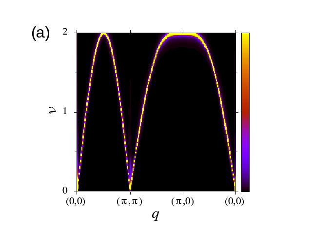
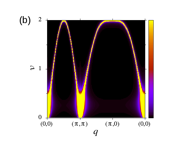
Figure 2: (Color online) Spin wave excitation in the AF plane for (a) non-correlated case, $g_{t}=1$, and (b) correlated case, $g_{t}$=$2p/(1+p)$ with $p$=0.01. (c) $\nu$-cuts of $Z(q,\nu)$ around ($\pi$,$\pi$) plotted for $\nu$=0.5 (blue solid line) and 1.0 (red solid line).

In the correlated case, on the other hand, it is clear that the low-energy region of the spectrum is broad as shown in Fig. 2(b). To see the broadening of the spectrum, their intensities are plotted in Fig. 2(c) for $\nu$=0.5 (blue solid line) and $\nu$=1.0 (red solid line). The broadening of the spectrum is marked in the low-energy region, i.e., $\nu\lesssim$ 0.5.

The imaginary part of $E_{-}(q,\nu)$, which corresponds to the width of spectrum $\Gamma$, is plotted in Fig. 3. Figure 3(a) shows the distribution of ${\rm Im}E_{-}(q,\nu)$ on the ($q$,$\nu$) plane, while several $\nu$-cuts for the correlated case with $p$=0.01 are plotted in Fig. 3(b).

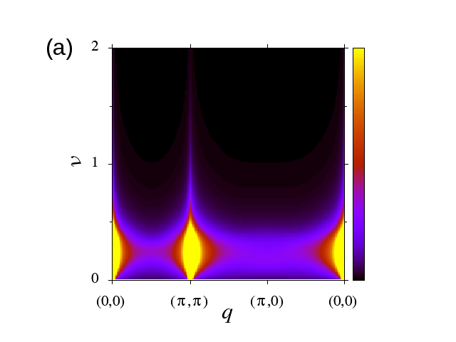
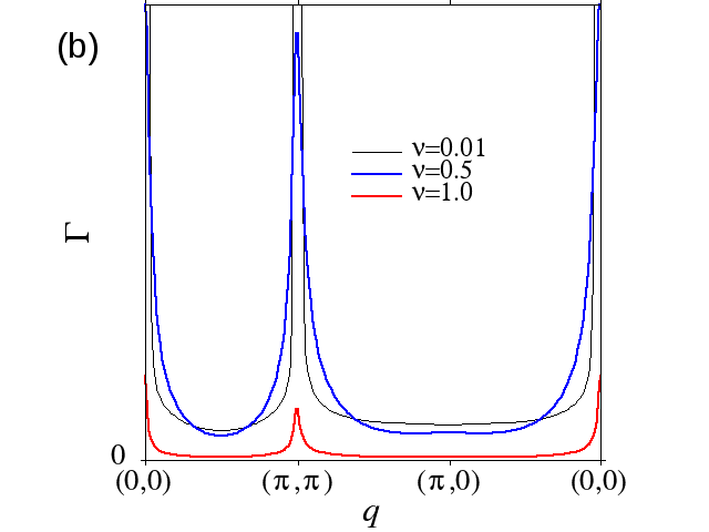
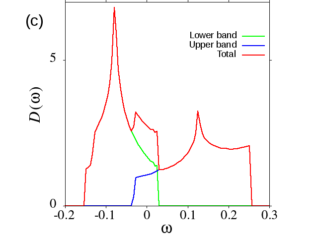
Figure 3: (Color online) (a) Imaginary part of $E_{-}(q,\nu)$, which corresponds to the width $\Gamma$, plotted in ($q$,$\nu$) plane for the correlated case with $p$=0.01. (b) $\nu$-cuts of Im$E_{-}(q,\nu)$ for $\nu$=0.01 (gray), 0.5 (blue), and 1.0 (red). (c) Density of states (DOS) in the CM with $p$=0.01. The dispersion relation of electrons in the CM is folded by the AF order. The DOS of the upper (lower) band is plotted by the blue (green) line. The total DOS, i.e., the sum of the upper and lower bands, is shown by the red line. The DOS of the non-correlated case is not shown here since its magnitude is two orders smaller than those shown in this figure.

Again, we can see that $\Gamma$ is large in the region of $\nu\lesssim$ 0.5, particularly around $\nu\sim$ 0.25, as shown in Fig. 3(a). In addition, the large $\Gamma$ is rather concentrated around (0,0) and ($\pi$,$\pi$) in Fig. 3(b). Here, the question may arise; why is the low-energy region so broad? To answer this question, the density of states, $D(\omega)$, in the CM is plotted in Fig. 3 (c) for $g_{t}$=$2p/(1+p)$ with $p$=0.01. The band in the CM is folded by the AF order in the AF plane, i.e., the last term in Eq. (7), and it comprises upper and lower bands. The AF order is assumed to be stable in this paper. It is important to note the suppression of the band width $W$ to $\sim$ 0.5 due to the Gutzwiller factor $g_{t}\sim$0.02. The magnitude of $D(\omega)$ is automatically enhanced to conserve the total number of states. In fact, $D(\omega)$ for the non-correlated case is two orders smaller than that for the correlated one and is not visible in Fig. 3 (c). Note that $\Sigma$ is composed of particle-hole excitations in the CM, which can be seen from Eqs. (40) and (41), which leads to $\Gamma$. When $W$ is suppressed and the magnitude of $D(\omega)$ is enhanced, the particle-hole excitations gain a large phase volume at low energies, i.e., $\omega\lesssim$ 0.5. In particular, the particle-hole excitations between the two peaks corresponding to the van Hove singularity in Fig. 3 (c) have the largest contribution, whose energy is about $\omega\sim$ 0.25. In fact, $\Gamma$ is large around $\nu\sim$0.25 as shown in Fig. 3 (a). In the non-correlated case with the same energy window $\sim$0.5, the phase volume of particle-hole excitations is two orders smaller than that in the correlated case since its band width is two orders larger than that in the correlated case. This is the reason why we could not see any broadening in Fig. 2(a). On the whole, $\Gamma$ is large around (0,0) and ($\pi$,$\pi$) as shown in Fig. 3(b). Since the origin of $\Gamma$ is particle-hole excitations in the CM, this enhancement implies the nesting of the Fermi surface near half-filling with the band folding.

So far, we have compared the non-correlated case, $g_{t}$=1, with only one correlated case, $g_{t}\sim$0.02 with $p$=0.01. A quantitative estimation of $\Gamma$ is necessary. In our results, the enhancement of $\Gamma$ originates from $g_{t}$ as a function of $p$, while $\Gamma$ depends on not only $g_{t}$ but also $q$ and $\nu$. In Fig. 4, $\Gamma$ is plotted as a function of $g_{t}$ for $q$=($\pi$,$\pi$), $\nu$=0.5, and $p$=0.01.

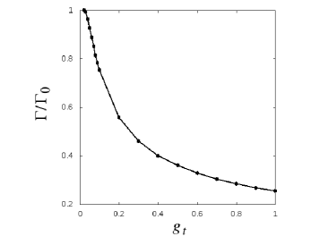
Figure 4: $\Gamma$ plotted as a function of $g_{t}$ for $q$=($\pi$,$\pi$), $\nu$=0.5. It is normalized by its magnitude at $g_{t}$=0.02, defined by $\Gamma_{0}$. Note that $p$ is fixed to 0.01 and $g_{t}$ is exceptionally assumed to be independent of $p$ in order to simulate the correlation effect on $\Gamma$.

It is normalized by its magnitude at $g_{t}$=0.02, defined by $\Gamma_{0}$, i.e., the peak height of the blue line at ($\pi$,$\pi$) in Fig. 3(b). Note that $g_{t}$ in Fig. 4 is exceptionally assumed to be independent of $p$. Figure 4 shows how $\Gamma$ is quantitatively enhanced by the correlation, i.e., $g_{t}$. It is found that $\Gamma$ increases with decreasing $g_{t}$. Roughly estimated, it is inversely proportional to $g_{t}$ since $\Gamma$ originates from the particle-hole excitations in the CM with the bandwidth suppressed by $g_{t}$.

The magnetic excitation spectrum can be measured by INS measurement, in which the spectrum is determined by the following correlation function:

$$\chi^{+-}(q,\nu) = \sum_{l}\sum_{\alpha,\beta=A,B}\int\frac{dt}{2\pi}e^{-i\nu t+iq{R_{l}}}\left\langle{S_{0\alpha}^{+}(0)S_{l\beta}^{-}(t)}\right\rangle,$$ (52)

$$= \frac{S}{\pi}\sum_{i,j=1,2}G_{i,j}(q,\nu).$$ (53)

Each component of the Green function in Eq. (49) is denoted by $G_{i,j}(q,\nu)$. In Fig. 5, Im $\chi^{+-}(q,\nu)$ is plotted for the correlated case $g_{t}=2p/(1+p)$ with $p$=0.01.

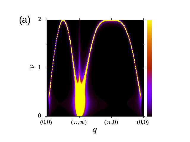
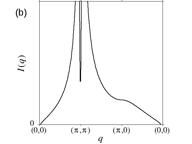
Figure 5: (Color online) (a) Imaginary part of spin-spin correlation function, $\chi^{+-}(q,\omega)$, which is observed by INS measurement, for the correlated case with $p$=0.01. (b) $\nu$-integrated intensity of $\chi^{+-}(q,\omega)$. The intensity is enhanced around ($\pi$,$\pi$), whereas it is suppressed around (0,0).

Compared with Fig. 2(b), the spectral weight is enhanced around ($\pi$,$\pi$), while it is suppressed around (0,0). The $\nu$-integrated intensity, defined by $I(q)\equiv\int d\nu~{}{\rm Im}~{}\chi^{+-}(q,\nu)$, is shown in Fig. 5(b). This is characteristic to the AF spin wave and is observed in cuprates headings . Since the INS measurement can observe the magnetic excitations around ($\pi$,$\pi$), the broad linewidth of the AF spin wave due to the electron correlation can be measured by INS.

IV Summary and Discussion

We have studied the magnetic excitations in the bilayer of an antiferromagnetic (AF) insulator and a correlated metal (CM), i.e., a doped Mott insulator, in which double occupancy is forbidden. The correlation effect in the metallic plane is treated by the Gutzwiller approximation, which renormalizes the hopping integrals proportional to the hole density. The effective action of a linearized AF spin wave in the AF insulator is calculated by second-order perturbation theory with respect to the interplane coupling. The path integral formula is useful to integrate out the electron degrees of freedom in the CM. Near half-filling, the strong repulsion between electrons suppresses their kinetic energy and results in a narrow band width, which gives enough phase space for low-energy magnetic excitations. The self-energy of an AF spin wave originates from the particle-hole excitation in the metallic plane. Hence, these excitations with a narrow band width make the AF spin wave broad at low energies due to the electron correlation. By increasing the correlation effect, i.e., by decreasing $g_{t}$, the linewidth at low energies increases inversely proportional to $g_{t}$.

In this paper, only the AF insulating plane was focused on, while we should also consider magnetic excitations in the metallic plane. Preceding theoretical studies showed that magnetic excitations will appear around incommensurate wave numbers related to the Fermi surface geometry yamase06 ; norman . In addition, the magnetic exchange interaction in the CM induces other phases such as antiferromagnetism, $d$-wave superconductivity (dSC), the flux phase, the singlet resonant valence bond (RVB) state, and so on. These states will also make the AF spin wave broad, while it will be different from the present case. In some cases, the spectral weight of an AF spin wave in the AF insulating plane will be reduced by solving magnetic excitations in both planes self-consistently. This might lead to the two components proposed in INS studies sato , which will be clarified in the near future.

If the CM plane is substituted by the dSC, such a bilayer system is a coexistent phase of AF and dSC, as observed in the multilayered cuprates by nuclear magnetic resonance (NMR) measurements mukuda12 . Simultaneously, the coexistence within one CuO₂ plane has also been observed by NMR measurements mukuda12 and theoretically studied inaba ; yamase ; hayashi13 . In addition, the phase separation between AF and dSC states may also be possiblekoikegami . Even though the magnetic excitations in these cases are not obvious, their situations are close to the present study. For example, in terms of a slave fermion with a large-$N$ expansion yoshioka , the nearest-neighbor hopping is associated with the interplane coupling in our bilayer model, and the metallic plane corresponds to the kinetic terms of the second- and third-neighbor hoppings. Hence, our results will also be useful to study the magnetic excitations in the coexistent and phase-separated phases.

Finally, it is also noted that the present model is closely related to some spintronics devices using a bilayer of a metal and a ferrimagnet, which is often referred to as a ferromagnet maekawa . For example, electricity can be generated by applying a temperature gradient to such a bilayer system. This is called the spin Seebeck effect, which is a completely new method of thermoelectric generation uchida08 ; adachi13 . The low-energy magnetic excitations and their lifetime are crucial to understand the experimental signal and to improve the efficiency of the spin Seebeck effect ohnuma ; kikkawa . The present results will contribute to such various research fields.

Appendix A Bilayer of $\bm{Ferri}$magnet and Metal

We show the effective action of linearized spin waves in a bilayer of a ferrimagnet and a (correlated) metal, which is often used in spintronics. The simplest model of a ferrimagnet is two sublattices with different magnitudes of magnetization $S_{A}\neq S_{B}$. Instead of Eq. (2), the Hamiltonian of the ferrimagnetic plane $\tilde{H}_{\rm I}$ is given by

$$\tilde{H}_{\rm I}=J\sum_{\left\langle{i,j}\right\rangle}\vec{S}_{i}\cdot\vec{S}_{j}-J_{A}\sum_{\left\langle{i,i^{\prime}}\right\rangle}\vec{S}_{i}\cdot\vec{S}_{i^{\prime}}-J_{B}\sum_{\left\langle{j,j^{\prime}}\right\rangle}\vec{S}_{j}\cdot\vec{S}_{j^{\prime}}.$$ (54)

Hence, the Hamiltonian in Eq. (5) is substituted by

$$\tilde{H}_{HP} = \tilde{H}_{e}+\tilde{H}_{\rm int}+\tilde{H}_{m}$$ (55)

$$\tilde{H}_{e} = H_{\rm CM}+J_{\perp}\left(S_{A}\sum_{i\in A}\sigma_{i}^{z}-S_{B}\sum_{j\in B}\sigma_{j}^{z}\right)$$ (56)

$$\tilde{H}_{\rm int} = {J_{\bot}}\left[{\sqrt{\frac{{{S_{A}}}}{2}}\sum\limits_{i\in A}{\left({{a_{i}}\sigma_{i}^{-}+a_{i}^{\dagger}\sigma_{i}^{+}}\right)}+\sqrt{\frac{{{S_{B}}}}{2}}\sum\limits_{j\in B}{\left({b_{j}^{\dagger}\sigma_{j}^{-}+{b_{j}}\sigma_{j}^{+}}\right)}}\right],$$ (57)

$$\tilde{H}_{m} = J\sum_{i,j}\left\{{\sqrt{{S_{A}}{S_{B}}}\left({{a_{i}}{b_{j}}+a_{i}^{\dagger}b_{j}^{\dagger}}\right)+{S_{B}}a_{i}^{\dagger}{a_{i}}+{S_{A}}b_{j}^{\dagger}{b_{j}}}\right\}$$ (58)

$$- J_{A}S_{A}\sum_{i,i^{\prime}}\left({a_{i}^{\dagger}{a_{i^{\prime}}}+a_{i^{\prime}}^{\dagger}{a_{i}}-a_{i}^{\dagger}{a_{i}}-a_{i^{\prime}}^{\dagger}{a_{i^{\prime}}}}\right)$$

$$- J_{B}S_{B}\sum_{j,j^{\prime}}\left({b_{j}^{\dagger}{b_{j^{\prime}}}+b_{j^{\prime}}^{\dagger}{b_{j}}-b_{j}^{\dagger}{b_{j}}-b_{j^{\prime}}^{\dagger}{b_{j^{\prime}}}}\right).$$

Therefore, the matrix elements in Eqs. (14), (28), and (33) are replaced by

$$\tilde{S}_{0} = \sum_{q,i\nu_{n}}\Phi^{\dagger}\left[\left(\begin{array}[]{*{20}{c}}-i\nu_{n}&0\\ 0&i\nu_{n}\end{array}\right)+\left(\begin{array}[]{*{20}{c}}z_{1}JS_{B}+z_{2}J_{A}S_{A}(1-\zeta_{q})&z_{1}J\sqrt{S_{A}S_{B}}\gamma_{q}\\ z_{1}J\sqrt{S_{A}S_{B}}\gamma_{q}&z_{1}JS_{A}+z_{2}J_{B}S_{B}(1-\zeta_{q})\end{array}\right)\right]\Phi,$$ (63)

$$\tilde{H}(k,i{\omega_{n}}) \equiv \left({\begin{array}[]{*{20}{c}}{{\eta_{k}}+{m_{A}}}&0&{{\varepsilon_{k}}}&0\\ 0&{{\eta_{k}}-{m_{A}}}&0&{{\varepsilon_{k}}}\\ {{\varepsilon_{k}}}&0&{{\eta_{k}}-{m_{B}}}&0\\ 0&{{\varepsilon_{k}}}&0&{{\eta_{k}}+{m_{B}}}\end{array}}\right),$$ (68)

$$\tilde{M}(q,i{\nu_{n}}) \equiv \left({\begin{array}[]{*{20}{c}}0&{{\lambda_{A}}a_{q}^{\dagger}(i{\nu_{n}})}&0&0\\ {{\lambda_{A}}{a_{q}}(-i{\nu_{n}})}&0&0&0\\ 0&0&0&{{\lambda_{B}}{b_{-q}}(-i{\nu_{n}})}\\ 0&0&{{\lambda_{B}}b_{-q}^{\dagger}(i{\nu_{n}})}&0\end{array}}\right),$$ (73)

with $\lambda_{A}\equiv{J_{\perp}}\sqrt{S_{A}/2\beta}$, $\lambda_{B}\equiv{J_{\perp}}\sqrt{S_{B}/2\beta}$, $m_{A}\equiv J_{\perp}S_{A}/2$, and $m_{B}\equiv J_{\perp}S_{B}/2$. Hence, the self-energy, Eq. (39), is written as

$$\tilde{\Sigma} = {J_{\bot}^{2}\sqrt{S_{A}S_{B}}}\sum_{q,i\nu_{n}}\Phi^{\dagger}\left(\begin{array}[]{*{20}{c}}C_{+}&D\\ D&C_{-}\end{array}\right)\Phi,$$ (76)

$$C_{+} = \sum_{k,i\omega}\frac{(i\Omega-\eta_{k+q}-m_{B})(i\omega-\eta_{k}+m_{B})}{\left(\left(i\Omega-\eta_{k+q}+m_{A}\right)\left(i\Omega-\eta_{k+q}-m_{B}\right)-\varepsilon_{k+q}^{2}\right)\left(\left(i\omega-\eta_{k}-m_{A}\right)\left(i\omega-\eta_{k}+m_{B}\right)-\varepsilon_{k}^{2}\right)},$$ (77)

$$C_{-} = \sum_{k,i\omega}\frac{(i\Omega-\eta_{k+q}+m_{A})(i\omega-\eta_{k}-m_{A})}{\left(\left(i\Omega-\eta_{k+q}+m_{A}\right)\left(i\Omega-\eta_{k+q}-m_{B}\right)-\varepsilon_{k+q}^{2}\right)\left(\left(i\omega-\eta_{k}-m_{A}\right)\left(i\omega-\eta_{k}+m_{B}\right)-\varepsilon_{k}^{2}\right)},$$ (78)

$$D = \sum_{k,i\omega}\frac{{{\varepsilon_{k+q}}{\varepsilon_{k}}}}{\left(\left(i\Omega-\eta_{k+q}+m_{A}\right)\left(i\Omega-\eta_{k+q}-m_{B}\right)-\varepsilon_{k+q}^{2}\right)\left(\left(i\omega-\eta_{k}-m_{A}\right)\left(i\omega-\eta_{k}+m_{B}\right)-\varepsilon_{k}^{2}\right)}.$$ (79)

In this paper, we do not discuss the lifetime of a spin wave in a ferrimagnet. We simply consider the spectral weight of its spin wave.

$$i\nu = \frac{1}{2}\left[\pm\left(\epsilon_{1}-\epsilon_{2}\right)+\sqrt{\left(\epsilon_{1}+\epsilon_{2}\right)^{2}-4\epsilon_{3}^{2}}\right],$$ (80)

$$\epsilon_{1} = z_{1}JS_{B}+z_{2}J_{A}S_{A}(1-\zeta_{q}),$$ (81)

$$\epsilon_{2} = z_{1}JS_{A}+z_{2}J_{B}S_{B}(1-\zeta_{q}),$$ (82)

$$\epsilon_{3} = z_{1}J\sqrt{S_{A}S_{B}}\gamma_{q},$$ (83)

$$\zeta_{q} \equiv \frac{1}{z_{2}}\sum_{\rm e_{i}}e^{i{\bf q}{\bf e}_{i}}.$$ (84)

It is assumed that the number of second neighbor sites of A- and B-sites $z_{2}$ are the same. It is useful to see the $\nu$-integrated spectral weight $I(q)$ shown in Fig. 6.

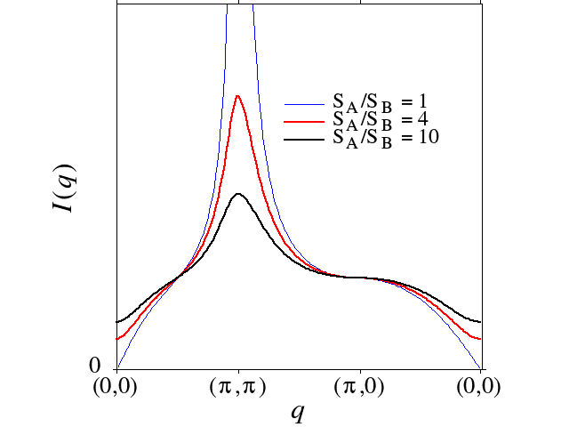
Figure 6: (Color online) $\nu$-integrated intensity of $\chi^{+-}(q,\omega)$ in the case of a ferrimagnet. Upon increasing the difference between sublattice magnetizations, the enhancement around ($\pi$,$\pi$) is suppressed and the intensity around (0,0) increases due to the opening of a gap.

For $S_{A}/S_{B}=1$, i.e., an antiferromagnet, $I(q)$ linearly decreases to zero around (0,0). This fact means that the spin current cannot be generated in the AF insulator ohnuma , whereas for the ferrimagnet such as one with $S_{A}/S_{B}=4$, the spectral weight around (0,0) becomes finite. This is caused by the degeneracy of the dispersion relation of spin waves. The spin waves in the AF insulator are degenerated, whereas those in the ferrimagnet are split with a magnitude of gap, $|S_{A}-S_{B}|$. Usually, the spin current is generated by an ac magnetic field, a temperature gradient, and so on. These external fields excite the magnons around (0,0). However, if we could excite the magnons around ($\pi$,$\pi$) by some means, it is obvious that the generated spin current could be a few orders of magnitudes larger than the conventional one obtained using a ferromagnet. This would be one of the strong merits of antiferromagnetic spintronics.

References

(1) P. A. Lee, N. Nagaosa, and X. G. Wen,
Rev. Mod. Phys. 78, 17 (2006).
(2) M. Ogata and H .Fukuyama,
Rep. Prog. Phys. 71, 036501 (2008).
(3) B. Keimer, S. A. Kivelson, M. R. Norman, S. Uchida, and J.
Zaanen,
Nature 518, 179 (2015).
(4)
D. Vaknin, S. K. Sinha, D. E. Moncton, D. L. Johnston, J. Newsam, and H.King,
Phys. Rev. Lett. 58, 2802 (1987).
(5)
K. Yamada, E. Kudo, Y. Endoh, Y. Hidaka, M. Oda, M. Suzuki, and T. Murakami,
Solid State Commun. 64, 753 (1987).
(6)
R. J. Birgeneau, D. R. Gabbe, H. P. Jenssen, M. A. Kastner,
P. J. Picone, T. R. Thurston, G. Shirane, Y. Endoh, M. Sato, K. Yamada, Y.
Hidaka, M. Oda, Y. Enomoto, M. Suzuki, and T. Murakami,
Phys. Rev. B 38, 6614 (1988).
(7)
S. M. Hayden, G. Aeppli, R. Osborn, A. D. Taylor, T. G.
Perring, S. W. Cheong, and Z. Fisk,
Phys. Rev. Lett. 67, 3622 (1991).
(8)
R. Coldea, S. M.Hayden, G. Aeppli, T. G. Perring, C. D. Frost, T. E. Mason,
S.-W. Cheong, and Z. Fisk,
Phys. Rev. Lett. 86, 5377 (2001).
(9) N. S. Headings, S. M. Hayden, R. Coldea, and T. G. Perring,
Phys. Rev. Lett. 105, 247001 (2010).
(10)
H. Yoshizawa, S. Mitsuda, H. Kitazawa, and K. Katsumata,
J. Phys. Soc. Jpn. 57, 3686 (1988).
(11)
G. Shirane, R. J. Birgeneau, Y. Endoh, P. Gehring, M. A. Kastner, K. Kitazawa,
H. Kojima, I. Tanaka, T. R. Thurston, and K. Yamada,
Phys. Rev. Lett. 63, 330 (1989).
(12)
K. Yamada, C. H. Lee, K. Kurahashi, J. Wada, S. Wakimoto, S.
Ueki, H. Kimura, Y. Endoh, S. Hosoya, G. Shirane, R. J. Birgeneau, M. Greven,
M. A. Kastner, and Y. J. Kim,
Phys. Rev. B 57, 6165 (1998).
(13)
J. M. Tranquada, H. Woo, T. G. Perring, H. Goka, G. D. Gu, G. Xu,
M. Fujita, and K. Yamada, Nature 429, 534 (2004).
(14) B. Vignolle, S. M. Hayden, D. F. McMorrow, H. M. Ronnow, B.
Lake, C. D. Frost, and T. G. Perring,
Nat. Phys. 3, 163 (2007).
(15)
D. Reznik, J.-P. Ismer, I. Eremin, L. Pintschovius, T. Wolf, M. Arai, Y. Endoh,
T. Masui, and S. Tajima,
Phys. Rev. B 78, 132503 (2008).
(16) O. J. Lipscombe, B. Vignolle, T. G. Perring, C. D. Frost,
and S. M. Hayden,
Phys. Rev. Lett. 102, 167002 (2009).
(17)
M. Fujita, H. Hiraka, M. Matsuda, M. Matsuura, J. M.
Tranquada, S. Wakimoto, G. Xu, and K. Yamada,
J. Phys. Soc. Jpn. 81, 011007 (2012).
(18)
M. R. Norman,
Phys. Rev. B 61, 14751 (2000).
(19)
H. Yamase and W. Metzner,
Phys. Rev. B 73, 214517 (2006).
(20) M. Le Tacon, G. Ghiringhelli, J. Chaloupka, M. Moretti
Sala, V. Hinkov, M. W. Haverkort, M. Minola, M. Bakr, K. J. Zhou, S.
Blanco-Canosa, C. Monney, Y. T. Song, G. L. Sun, C. T. Lin, G. M. De
Luca, M. Salluzzo, G. Khaliullin, T. Schmitt, L. Braicovich, and B.
Keimer, Nat. Phys. 7, 725 (2011).
(21) M. Matsuura, S. Kawamura, M. Fujita, R. Kajimoto, and K.
Yamada, Phys. Rev. B 95, 024504 (2017).
(22) K. Sato, M. Matsuura, K. Ikeuchi, R. Kajimoto, S. Wakimoto, and
M. Fujita, private communication.
(23) S. P. Bayrakci, T. Keller, K. Habicht, and B. Keimer,
Science 312, 1926 (2006).
(24) S. P. Bayrakci, D. A. Tennant, Ph. Leininger, T. Keller,
M. C. R. Gibson, S. D. Wilson, R. J. Bergeneau, and B. Keimer,
Phys. Rev. Lett. 111, 017204 (2013).
(25) K. F. Tseng, T. Keller, A. C. Walters, R. J. Birgeneau, and B.
Keimer, Phys. Rev. B 94, 014424 (2016).
(26) A. B. Harris, D. Kumar, B. I. Halperin, and P. C.
Hohenberg, Phys. Rev. B 3, 961 (1971).
(27) B. I. Halperin and P.C. Hohenberg,
Phys. Rev. 188, 898 (1969).
(28) S. Ty and B. I. Halperin, Phys. Rev. B 42, 2096 (1990).
(29) A. V. Chubukov, J. J. Betouras, and D. V. Efremov, Phys.
Rev. Lett. 112, 037202 (2014).
(30) J. Kondo, J. Phys. Soc. Jpn. 58, 2884 (1989).
(31) M. Di Stasio, K. A. Müller, and L. Pietronero, Phys. Rev.
Lett. 64, 2827 (1990).
(32) A. Trokiner, L. Le Noc, J. Schneck, A. M. Pougnet, R.
Mellet, J. Primot, H. Savary, Y. M. Gao, and S. Aubry,
Phys. Rev. B 44, 2426 (1991).
(33) H. Mukuda, S. Shimizu, A. Iyo, and Y. Kitaoka,
J. Phys. Soc. Jpn. 81, 011008 (2012).
(34) M. Mori, T. Tohyama, and S. Maekawa,
Phys. Rev. B 66, 064502 (2002).
(35) M. Mori and S. Maekawa,
Phys. Rev. Lett. 94, 137003 (2005).
(36) M. Mori, T. Tohyama, and S. Maekawa,
J. Phys. Soc. Jpn. 75, 034708 (2006).
(37) K. Uchida, S. Takahashi, K. Harii, J. Ieda, W. Koshibae, K.
Ando, S. Maekawa, and E. Saitoh, Nature 455, 778 (2008)
(38) H. Adachi, K. Uchida, E. Saitoh, and S. Maekawa, Rep. Prog.
Phys. 76, 036501 (2013) and references therein.
(39) Y. Ohnuma, H. Adachi, E. Saitoh, and S. Maekawa,
Phys. Rev. B 87, 014423 (2013).
(40) T. Kikkawa, K. Uchida, S. Daimon, Z. Qiu, Y. Shiomi, and
E. Saitoh, Phys. Rev. B 92, 064413 (2015).
(41)
S. Geprags, A. Kehlberger, F. D. Coletta, Z. Qiu, E. J. Guo, T. Schulz, C.
Mix, S. Meyer, A. Kamra, M. Althammer, H. Huebl, G. Jakob, Y. Ohnuma, H.
Adachi, J. Barker, S. Maekawa, G. E. W. Bauer, E. Saitoh, R. Gross, S. T.
B.
Goennenwein,
and M. Klaui,
Nat. Commun. 7, 10452 (2016).
(42) N. Nagaosa, Quantum Field Theory in Condensed Matter
Physics (Springer, Berlin Heidelberg, 2010).
(43) M. Inaba, H. Matsukawa, and H. Fukuyama,
Physica C 257, 299 (1996).
(44) H. Yamase, M. Yoneya, and K. Kuboki,
Phys. Rev. B 84, 014508 (2011).
(45) M. Hayashi, Y. Tanuma, and K. Kuboki,
J. Phys. Soc. Jpn. 82, 124705 (2013).
(46) S. Koikegami, M. Kato, and T. Yanagisawa,
J. Phys. Soc. Jpn. 84, 054704 (2015).
(47) D. Yoshioka, J. Phys. Soc. Jpn. 58, 1516 (1989).
(48) S. Maekawa, S. O. Valenzuela, E. Saitoh, and T. Kimura, Spin Current, (Oxford University Press, Oxford, U.K., 2012).