Two-channel Kondo Effect Emerging from Nd Ions

Abstract

We discuss Kondo phenomena in a seven-orbital impurity Anderson model hybridized with $\Gamma_{8}$ conduction electrons by employing a numerical renormalization group method. In particular, we focus on the case with three local $f$ electrons, corresponding to a Nd³⁺ ion. For realistic values of Coulomb interactions, spin-orbit coupling, cubic crystalline electric field potentials, and hybridization, we find a residual entropy of $0.5\log 2$, a characteristic of two-channel Kondo phenomena, for the wide range of parameters of the local $\Gamma_{6}$ ground state. This is considered to be the magnetic two-channel Kondo effect, consistent with the result from an extended $s$-$d$ model constructed on the basis of the $j$-$j$ coupling scheme. Finally, we briefly discuss candidates of Nd compounds to observe the two-channel Kondo effect.

It is one of the fascinating problems in the modern condensed matter physics to realize an exotic new quantum state in strongly correlated electron systems. Among them, concerning the non-Fermi liquid state, the two-channel Kondo effect has been discussed for a long time as it is a confirmed route to arrive at the non-Fermi liquid ground state. Coqblin and Schrieffer derived exchange interactions from the multiorbital Anderson model.[1] Then, the concept of the multichannel Kondo effect was developed on the basis of such exchange interactions,[2] as a potential source of non-Fermi liquid phenomena. Moreover, such non-Fermi liquid properties were pointed out in a two-impurity Kondo system.[3, 4]

Concerning the reality of two-channel Kondo phenomena, Cox pointed out the existence of two screening channels in the case of quadrupole degrees of freedom in a cubic U compound with a $\Gamma_{3}$ non-Kramers doublet ground state.[5, 6] As Cox’s idea attracted significant attention, a large number of works were published on this topic and the understanding on the two-channel Kondo phenomena was considerably promoted. For instance, the roles of crystalline electric field (CEF) potentials were vigorously discussed. [7, 8, 9, 10, 11, 12, 13, 14, 15, 16, 17, 18] In order to observe the two-channel Kondo effect, first, experiments were performed in cubic U compounds and then Pr compounds with a $\Gamma_{3}$ non-Kramers doublet ground state were extensively investigated. Recently, in PrT₂X₂₀ compounds,[19] there were significant advances to grasp signs of non-Fermi liquid behavior. [20, 21, 22, 23] Theoretical research on this issue was also performed.[24, 25]

At present, research on the two-channel Kondo phenomena is nearly equivalent to that on the quadrupole two-channel Kondo effect. However, the magnetic two-channel Kondo effect should also be discussed in actual materials, when we come back to the original idea of Noziéres and Blandin. In addition, when we try to observe the two-channel Kondo effect, the number of candidate materials is limited; thus, it is necessary to develop Pr compounds with a $\Gamma_{3}$ non-Kramers doublet ground state. We believe that it is meaningful to push forward the research frontier of the two-channel Kondo physics to other rare-earth compounds.

In this study, we suggest that Nd compounds can provide a new stage of two-channel Kondo phenomena. We numerically analyze a seven-orbital impurity Anderson model hybridized with $\Gamma_{8}$ conduction electrons for the case with three local $f$ electrons corresponding to a Nd³⁺ ion. Then, we find a residual entropy of $0.5\log 2$ as a clear signal of the two-channel Kondo effect, for the case of the local $\Gamma_{6}$ ground state. By analyzing the $\Gamma_{6}$ state on the basis of the $j$-$j$ coupling scheme, we propose an extended $s$-$d$ model to explain the present result. Finally, we provide a few comments on the candidate materials to detect the two-channel Kondo effect.

First, we define the local $f$-electron Hamiltonian as

$$\begin{split}H_{\rm loc}&=\sum_{m_{1}\sim m_{4}}\sum_{\sigma,\sigma^{\prime}}I_{m_{1}m_{2},m_{3}m_{4}}f_{m_{1}\sigma}^{{\dagger}}f_{m_{2}\sigma^{\prime}}^{{\dagger}}f_{m_{3}\sigma^{\prime}}f_{m_{4}\sigma}\\ &+\lambda\sum_{m,\sigma,m^{\prime},\sigma^{\prime}}\zeta_{m,\sigma;m^{\prime},\sigma^{\prime}}f_{m\sigma}^{{\dagger}}f_{m^{\prime}\sigma^{\prime}}\\ &+\sum_{m,m^{\prime},\sigma}B_{m,m^{\prime}}f_{m\sigma}^{{\dagger}}f_{m^{\prime}\sigma}+E_{f}n,\end{split}$$ (1)

where $f_{m\sigma}$ is the annihilation operator for a local $f$ electron with spin $\sigma$ and $z$-component $m$ of angular momentum $\ell=3$, $\sigma=+1$ ($-1$) for up (down) spin, $I$ indicates Coulomb interactions, $\lambda$ is the spin-orbit coupling, $B_{m,m^{\prime}}$ denotes the CEF potentials, $E_{f}$ is the $f$-electron level, and $n$ denotes the local $f$-electron number.

The Coulomb interaction $I$ is expressed as

$$I_{m_{1}m_{2},m_{3}m_{4}}=\sum_{k=0}^{6}F^{k}c_{k}(m_{1},m_{4})c_{k}(m_{2},m_{3}),$$ (2)

where $F^{k}$ indicates the Slater-Condon parameter and $c_{k}$ is the Gaunt coefficient.[26] The sum is limited by the Wigner-Eckart theorem to $k=0$, $2$, $4$, and $6$. Although the Slater-Condon parameters of a material should be determined from experimental results, here, we set the ratio as

$$F^{0}/10=F^{2}/5=F^{4}/3=F^{6}=U,$$ (3)

where $U$ is the Hund rule interaction among $f$ orbitals.

Each matrix element of $\zeta$ is given by

$$\begin{split}\zeta_{m,\sigma;m,\sigma}&=m\sigma/2,\\ \zeta_{m+\sigma,-\sigma;m,\sigma}&=\sqrt{\ell(\ell+1)-m(m+\sigma)}/2,\end{split}$$ (4)

and zero for other cases. The CEF potentials for $f$ electrons from ligand ions are given in the table of Hutchings for the angular momentum $\ell=3$.[27] For a cubic structure with $O_{\rm h}$ symmetry, $B_{m,m^{\prime}}$ is expressed by two CEF parameters, $B_{4}^{0}$ and $B_{6}^{0}$, as

$$\begin{split}B_{3,3}&=B_{-3,-3}=180B_{4}^{0}+180B_{6}^{0},\\ B_{2,2}&=B_{-2,-2}=-420B_{4}^{0}-1080B_{6}^{0},\\ B_{1,1}&=B_{-1,-1}=60B_{4}^{0}+2700B_{6}^{0},\\ B_{0,0}&=360B_{4}^{0}-3600B_{6}^{0},\\ B_{3,-1}&=B_{-3,1}=60\sqrt{15}(B_{4}^{0}-21B_{6}^{0}),\\ B_{2,-2}&=300B_{4}^{0}+7560B_{6}^{0}.\end{split}$$ (5)

Note the relation $B_{m,m^{\prime}}=B_{m^{\prime},m}$. Following the traditional notation,[28] we define $B_{4}^{0}$ and $B_{6}^{0}$ as

$$B_{4}^{0}=Wx/F(4),~{}B_{6}^{0}=W(1-|x|)/F(6),$$ (6)

where $x$ specifies the CEF scheme for the $O_{\rm h}$ point group, while $W$ determines the energy scale for the CEF potential. We choose $F(4)=15$ and $F(6)=180$ for $\ell=3$.[27]

Now, we consider the case of $n=3$ by appropriately adjusting the value of $E_{f}$. As $U$ denotes the magnitude of the Hund rule interaction among $f$ orbitals, it is reasonable to set $U=1$ eV. The magnitude of $\lambda$ varies between 0.077 and 0.36 eV depending on the type of lanthanide ions. For a Nd³⁺ ion, $\lambda$ is $870-885$ cm^-1.[29] Thus, we set $\lambda=0.11$ eV. Finally, the magnitude of $W$ is typically of the order of millielectronvolts, although it depends on the material. Here, we simply set $|W|=10^{-3}$ eV.

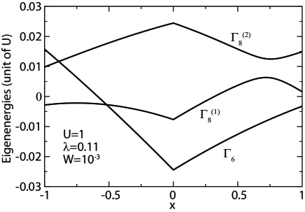
Figure 1: Low-lying eigenenergies of $H_{\rm loc}$ versus $x$ for $n=3$.

In Fig. 1, we depict curves of ten low-lying eigenenergies of $H_{\rm loc}$ for $n=3$ since the ground-state multiplet for $W=0$ is characterized by $J=9/2$, where $J$ denotes the total angular momentum of multi-$f$-electron state. We appropriately shift the origin of the energy to show all the curves in the present energy range. We emphasize that the results are almost the same as those of the $LS$ coupling scheme.[28] For the case of $W>0$, we find the $\Gamma_{8}^{(1)}$ ground state for $x\leq-0.5$, while the $\Gamma_{6}$ ground state is observed for $x\geq-0.5$. However, for $W<0$, the $\Gamma_{6}$ ground state appears only in the vicinity of $x=-1.0$. For the wide range of $-0.9<x\leq 1$, we obtain another $\Gamma_{8}^{(2)}$ ground state.

Now, we include $\Gamma_{8}$ conduction bands hybridized with localized $f$ electrons. For the purpose, it is convenient to transform the $f$-electron basis in $H_{\rm loc}$ from $(m,\sigma)$ to $(j,\mu,\tau)$, where $j$ denotes the total angular momentum of one $f$-electron state, $\mu$ indicates the irreducible representation of $O_{\rm h}$ point group, and $\tau$ denotes the pseudo-spin to distinguish the Kramers degenerate state. For $j=7/2$ octet, we have two doublets ($\Gamma_{6}$ and $\Gamma_{7}$) and one quartet ($\Gamma_{8}$), while for $j=5/2$ sextet, we obtain one doublet ($\Gamma_{7}$) and one quartet ($\Gamma_{8}$). In the present case, we consider the hybridization between $\Gamma_{8}$ conduction electrons and the $\Gamma_{8}$ quartet of $j=5/2$.

Then, the seven-orbital Anderson model is expressed as

$$H\!=\!\!\sum_{\mib{k},\mu,\tau}\!\varepsilon_{\mib{k}}c_{\mib{k}\mu\tau}^{{\dagger}}c_{\mib{k}\mu\tau}\!+\!\!\sum_{\mib{k},\mu,\tau}\!V(c_{\mib{k}\mu\tau}^{{\dagger}}\tilde{f}_{5/2\mu\tau}+{\rm h.c.})\!+\!\tilde{H}_{\rm loc},$$ (7)

where $\varepsilon_{\mib{k}}$ is the dispersion of a conduction electron with wave vector $\mib{k}$, $c_{\mib{k}\mu\tau}$ is the annihilation operator of a $\Gamma_{8}$ conduction electron, $\mu$ (=$\alpha$ and $\beta$) distinguishes the $\Gamma_{8}$ quartet, $\tau$ (=$\uparrow$ and $\downarrow$) is the pseudo-spin, ${\tilde{f}}_{j\mu\tau}$ is the annihilation operator of a localized $f$ electron expressed by the bases of $(j,\mu,\tau)$, $V$ is the hybridization between conduction and localized electrons, and $\tilde{H}_{\rm loc}$ is obtained from $H_{\rm loc}$ by the transformation of the $f$-electron basis from $(m,\sigma)$ to $(j,\mu,\tau)$.

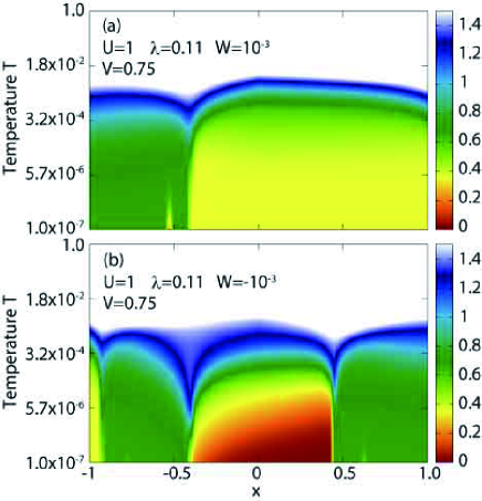
Figure 2: (Color online) Contour color map of the entropy on the plane of $x$ and $T$ for (a) $W=10^{-3}$ and (b) $W=-10^{-3}$. Note that $T$ is given in a logarithmic scale.

In this study, we analyze the model by employing a numerical renormalization group (NRG) method.[30, 31] We introduce a cut-off $\Lambda$ for the logarithmic discretization of the conduction band. Owing to the limitation of computer resources, we keep $M$ low-energy states. Here, we use $\Lambda=5$ and $M=4,000$. In the following calculations, the energy unit is $D$, which is a half of the conduction band width. Namely, we set $D=U=1$ eV in this calculation. In the NRG calculation, the temperature $T$ is defined as $T=\Lambda^{-(N-1)/2}$ in the present energy unit, where $N$ is the number of renormalization steps.

In Fig. 2(a), we show the contour color map of the entropy for $W=10^{-3}$ and $V=0.75$. To visualize precisely the behavior of entropy, we define the color of the entropy between $0$ and $1.5$, as shown in the right color bar. We immediately notice that an entropy of $\log 2$ (green region) appears at low temperatures for $-1.0<x<-0.4$, while an entropy of $0.5\log 2$ (yellow region) is found for $-0.4<x<1.0$. The region with an entropy of $0.5\log 2$ almost corresponds to that of the $\Gamma_{6}$ ground state in comparison with Fig. 1, although we find a small difference between them around $x\sim 0.5$. The residual entropies, $0.5\log 2$ and $\log 2$, are eventually released at extremely low temperatures in the numerical calculations. Approximately at $x=-0.5$, the release of an entropy of $\log 2$ seems to occur at relatively high temperatures. This is considered to be related with the accidental degeneracy of $\Gamma_{6}$ and $\Gamma_{8}^{(1)}$ states. In any case, the details on the entropy behavior at low temperatures will be discussed elsewhere in the future.

In Fig. 2(b), we show the contour color map of the entropy for $W=-10^{-3}$ and $V=0.75$. Again, we find a residual entropy of $0.5\log 2$ in the vicinity of $x=-1.0$, just corresponding to the region of the $\Gamma_{6}$ ground state for $W<0$, as observed in Fig. 1. For $-0.9<x<1$, the CEF ground state is $\Gamma_{8}^{(2)}$, but depending on the excited states, the entropy behavior is different. We find the singlet ground state between $-0.5<x<0.5$, while a residual entropy of $\log 2$ appears for $-0.9<x<-0.5$ and $0.5<x<1$. For the case of the $\Gamma_{8}^{(2)}$ ground state, we do not find a residual entropy of $0.5\log 2$ even at a certain point of $x$. Thus, from Figs. 2(a) and 2(b), we conclude that a residual entropy of $0.5\log 2$ appears for the case of the $\Gamma_{6}$ ground state for $f^{3}$ systems. The Kondo effect for the case of the $\Gamma_{8}^{(2)}$ ground state is considered to be related to that in the model with an impurity spin hybridized with conduction electrons with spin $3/2$.[32, 33] The point will be also discussed elsewhere in the future.

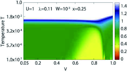
Figure 3: (Color online) Contour color map of the entropy on the $(V,T)$ plane for $x=0.25$ and $W=10^{-3}$.

Next we discuss the $V$ dependence of the entropy. In Fig. 3, we show the contour color map of the entropy on the $(V,T)$ plane for $x=0.25$ and $W=10^{-3}$ with the $\Gamma_{6}$ local ground state. We emphasize that the $0.5\log 2$ entropy does not appear only at a certain value of $V$, but it can be observed in the wide region of $V$ such as $0.6<V<0.9$ in the present temperature range. This behavior is different from that in the non-Fermi liquid state because of the competition between the CEF and Kondo-Yosida singlets for $f^{2}$ systems.[14, 17, 18] Additionally, the two-channel Kondo effect appears for relatively large values of $V$ in the energy scale of $U=D=1$ eV.

We believe that the two-channel Kondo effect is confirmed to occur for the case of $n=3$ with the local $\Gamma_{6}$ ground state in the NRG calculation for the seven-orbital Anderson model. However, it is difficult to describe the electronic state from a microscopic viewpoint as all $f$ orbitals are included in the present calculations. Thus, it is desirable to consider the effective model including only $j=5/2$ states to grasp the essential point of the electronic states.[34] For the purpose, we exploit the $j$-$j$ coupling scheme to derive the effective potentials and interactions among $j=5/2$ states by the perturbation expansion in terms of $1/\lambda$.[35] Then, we perform the NRG calculations for the three-orbital Anderson model hybridized with $\Gamma_{8}$ conduction bands by using the same parameters as those in Fig. 2(a). Then, we obtain almost the same contour map of entropy on the $(x,T)$ plane (not shown here) by using the $j$-$j$ coupling scheme with the effective interactions.

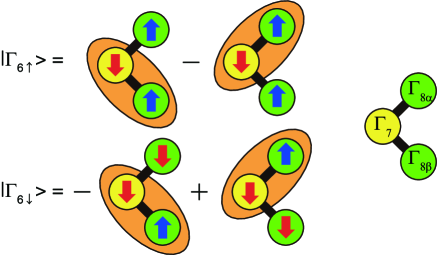
Figure 4: (Color online) Schematic views of $\Gamma_{6}$ states composed of the three pseudo-spins on $\Gamma_{7}$, $\Gamma_{8\alpha}$, and $\Gamma_{8\beta}$ orbitals of $j=5/2$. The oval denotes the singlet between $\Gamma_{7}$ and $\Gamma_{8}$ states. The right figure shows the configuration of $\Gamma_{7}$, $\Gamma_{8\alpha}$, and $\Gamma_{8\beta}$ orbitals.

Now we consider the local $\Gamma_{6}$ state on the basis of the $j$-$j$ coupling scheme. After some algebraic calculations, we express $\Gamma_{6}$ states by using the three spins on $\Gamma_{7}$ and $\Gamma_{8}$ orbitals, as schematically shown in Fig. 4. Namely, we obtain [36]

$$\begin{split}|\Gamma_{6},\uparrow\rangle&=\frac{1}{\sqrt{3}}\left({\tilde{f}}^{{\dagger}}_{5/2\alpha\uparrow}|S_{78\beta}\rangle-{\tilde{f}}^{{\dagger}}_{5/2\beta\uparrow}|S_{78\alpha}\rangle\right),\\ |\Gamma_{6},\downarrow\rangle&=\frac{1}{\sqrt{3}}\left(-{\tilde{f}}^{{\dagger}}_{5/2\alpha\downarrow}|S_{78\beta}\rangle+{\tilde{f}}^{{\dagger}}_{5/2\beta\downarrow}|S_{78\alpha}\rangle\right),\end{split}$$ (8)

where $|S_{78\mu}\rangle$ denotes the singlet state, given by

$$|S_{78\mu}\rangle=\frac{1}{\sqrt{2}}\left({\tilde{f}}^{{\dagger}}_{5/2\gamma\uparrow}{\tilde{f}}^{{\dagger}}_{5/2\mu\downarrow}-{\tilde{f}}^{{\dagger}}_{5/2\gamma\downarrow}{\tilde{f}}^{{\dagger}}_{5/2\mu\uparrow}\right)|0\rangle.$$ (9)

Here, ${\tilde{f}}_{5/2\gamma\tau}$ is the annihilation operator of $\Gamma_{7}$ electron and $|0\rangle$ denotes the vacuum. The main component of the $\Gamma_{3}$ non-Kramers doublet state of $n=2$ is expressed by $|S_{78\alpha}\rangle$ and $|S_{78\beta}\rangle$. Thus, the $\Gamma_{6}$ states of $n=3$ are obtained by the addition of one $\Gamma_{8}$ electron to $\Gamma_{3}$ states of $n=2$. We intuitively understand that the pseudo-spin properties of $\Gamma_{6}$ originate from those of $\Gamma_{8}$ electrons.

On the basis of local $\Gamma_{6}$ states composed of the three pseudo-spins, we obtain an extended $s$-$d$ model, given by

$$H\!=\!\!\!\sum_{\mib{k},\mu,\tau}\!\!\varepsilon_{\mib{k}}c_{\mib{k}\mu\tau}^{{\dagger}}c_{\mib{k}\mu\tau}\!+\!J_{1}\!\!\!\sum_{\mu=\alpha,\beta}\!\!\mib{s}_{\mu}\cdot\mib{S}_{8\mu}\!+\!J_{2}\!\!\!\sum_{\mu=\alpha,\beta}\!\!\mib{S}_{7}\cdot\mib{S}_{8\mu},$$ (10)

where $J_{1}$ is the Kondo exchange coupling, $J_{2}$ denotes the effective negative Hund rule coupling among $\Gamma_{7}$ and $\Gamma_{8}$ orbitals,[36] $\mib{s}_{\mu}$ denotes the conduction electron spin for the $\mu$ orbital, and $\mib{S}_{7}$ and $\mib{S}_{8\mu}$ indicate the local spin on $\Gamma_{7}$ and $\Gamma_{8\mu}$ orbitals, respectively.

In Fig. 5, we show the typical results of the entropy and specific heat of the extended $s$-$d$ model with $J_{1}=0.5$ and $J_{2}=0.1$. We clearly find a residual entropy of $0.5\log 2$ at low temperatures, suggesting the emergence of the two-channel Kondo effect. In contrast to the well-known two-channel Kondo model, we observe a remnant of the plateau of $\log 2$ before entering the two-channel Kondo region. Corresponding to the change of the entropy, we observe a small peak in the specific heat. Here, we show only the results for $J_{1}=0.5$ and $J_{2}=0.1$, but the two-channel Kondo behavior can be widely observed for positive values of $J_{1}$ and $J_{2}$.

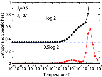
Figure 5: (Color online) Entropy and specific heat of the extended $s$-$d$ model for $J_{1}=0.5$ and $J_{2}=0.1$.

Now, we briefly discuss the candidate $f^{3}$ materials to observe the two-channel Kondo behavior. A simple way is to search Nd cubic compounds with $\Gamma_{6}$ ground states. For the purpose, it is convenient to synthesize Nd compounds with the same crystal structure as that of Pr compounds with a $\Gamma_{3}$ non-Kramers ground state from the discussion on the CEF states for $n=2$ and $3$. As we have remarked in Fig. 3, to observe the two-channel Kondo effect in $f^{3}$ systems, it is necessary to consider relatively large hybridization, suggesting that a rare-earth ion should be surrounded by many ligand ions. In this sense, good candidates are considered to be Nd 1-2-20 compounds, such as NdIr₂Zn₂₀,[37] NdRh₂Zn₂₀, NdV₂Al₂₀,[38] and NdTi₂Al₂₀,[39, 40] since corresponding Pr compounds are known to exhibit $\Gamma_{3}$ non-Kramers doublets.[19]

Among them, the $\Gamma_{6}$ ground state has been confirmed for NdIr₂Zn₂₀,[37] but the signals of the two-channel Kondo effect have not been reported. At low temperatures, antiferromagnetic phases have been observed for NdIr₂Zn₂₀ [37] and NdTi₂Al₂₀,[40] while a ferromagnetic phase has been found for NdV₂Al₂₀.[38] Thus, a high pressure can be applied to such magnetic phases since we expect a chance to observe the two-channel Kondo behavior if we obtain a metallic phase through the quantum critical point under a high pressure.

Another candidate may be found in Np cubic compounds with a Np⁴⁺ ion including three $5f$ electrons because in general, the itinerant nature of $5f$ electrons is large in comparison with that of $4f$ electrons. However, as the treatment of Np compounds is strictly limited, it may be difficult to find the two-channel Kondo behavior in Np cubic compounds.

In summary, we found the two-channel Kondo effect in the seven-orbital impurity Anderson model hybridized with $\Gamma_{8}$ conduction electrons for the case of $n=3$ with the local $\Gamma_{6}$ ground state. To detect the two-channel Kondo effect emerging from Nd ions, we proposed to perform the experiments using Nd 1-2-20 compounds.

The author thanks Y. Aoki, K. Hattori, R. Higashinaka, K. Kubo, and T. Matsuda for discussions on heavy-electron systems. This work was supported by JSPS KAKENHI Grant Number JP16H04017. The computation in this work was done using the facilities of the Supercomputer Center of Institute for Solid State Physics, University of Tokyo.

References

- [1] B. Coqblin and J. R. Schrieffer, Phys. Rev. 185, 847 (1969).
- [2] Ph. Noziéres and A. Blandin, J. Physique 41, 193 (1980).
- [3] B. A. Jones and C. M. Varma, Phys. Rev. Lett. 58, 843 (1987).
- [4] B. A. Jones, C. M. Varma, and J. W. Wilkins, Phys. Rev. Lett. 61, 125 (1988).
- [5] D. L. Cox, Phys. Rev. Lett. 59, 1240 (1987).
- [6] D. L. Cox and A. Zawadowski, Exotic Kondo Effects in Metals (Taylor & Francis, London, 1999), p. 24.
- [7] M. Koga and H. Shiba, J. Phys. Soc. Jpn. 64, 4345 (1995).
- [8] M. Koga and H. Shiba, J. Phys. Soc. Jpn. 65, 3007 (1996).
- [9] H. Kusunose and K. Miyake, J. Phys. Soc. Jpn. 66, 1180 (1997).
- [10] H. Kusunose, J. Phys. Soc. Jpn. 67, 61 (1998).
- [11] Y. Shimizu, O. Sakai, and S. Suzuki, J. Phys. Soc. Jpn. 67, 2395 (1998).
- [12] M. Koga, G. Zaránd, and D. L. Cox, Phys. Rev. Lett. 83, 2421 (1999).
- [13] M. Koga, Phys. Rev. B 61, 395 (2000).
- [14] S. Yotsuhashi, K. Miyake, and H. Kusunose, J. Phys. Soc. Jpn. 71, 389 (2002).
- [15] K. Hattori and K. Miyake, J. Phys. Soc. Jpn. 74, 2193 (2005).
- [16] M. Koga and M. Matsumoto, Phys. Rev. B 77, 094411 (2008).
- [17] S. Nishiyama, H. Matsuura, and K. Miyake, J. Phys. Soc. Jpn. 79, 104711 (2010).
- [18] S. Nishiyama and K. Miyake, J. Phys. Soc. Jpn. 80, 124706 (2011).
- [19] See, for instance, T. Onimaru and H. Kusunose, J. Phys. Soc. Jpn. 85, 082002 (2016) and references therein.
- [20] A. Sakai and S. Nakatsuji, J. Phys. Soc. Jpn. 80, 063701 (2011).
- [21] T. Onimaru, K. T. Matsumoto, Y. F. Inoue, K. Umeo, Y. Saiga, Y. Matsushita, R. Tamura, K. Nishimoto, I. Ishii, T. Suzuki, and T. Takabatake, J. Phys. Soc. Jpn. 79, 033704 (2010).
- [22] T. Onimaru, K. T. Matsumoto, Y. F. Inoue, K. Umeo, T. Sakakibara, Y. Karaki, M. Kubota, and T. Takabatake, Phys. Rev. Lett. 106, 177001 (2011).
- [23] R. Higashinaka, A. Nakama, M. Ando, M. Watanabe, Y. Aoki, and H. Sato, J. Phys. Soc. Jpn. 80, SA048 (2011).
- [24] A. Tsuruta and K. Miyake, J. Phys. Soc. Jpn. 84, 114714 (2015)
- [25] H. Kusunose, J. Phys. Soc. Jpn. 85, 064708 (2016).
- [26] J. C. Slater, Quantum Theory of Atomic Structure (McGraw-Hill, New York, 1960).
- [27] M. T. Hutchings, Solid State Phys. 16, 227 (1964).
- [28] K. R. Lea, M. J. M. Leask, and W. P. Wolf, J. Phys. Chem. Solids 23, 1381 (1962).
- [29] W. T. Carnall, P. R. Fields, and K. Rajnak, J. Chem. Phys. 49, 4424 (1968).
- [30] K. G. Wilson, Rev. Mod. Phys. 47, 773 (1975).
- [31] H. R. Krishna-murthy, J. W. Wilkins, and K. G. Wilson, Phys. Rev. B 21, 1003 (1980).
- [32] T. S. Kim, L. N. Oliveira, and D. L. Cox, Phys. Rev. B 55, 12460 (1997).
- [33] K. Hattori, J. Phys. Soc. Jpn. 74, 3135 (2005).
- [34] T. Hotta and K. Ueda, Phys. Rev. B 67, 104518 (2003).
- [35] T. Hotta and H. Harima, J. Phys. Soc. Jpn. 75, 124711 (2006).
- [36] K. Kubo and T. Hotta, Phys. Rev. B 95, 054425 (2017).
- [37] Y. Yamane, R. Yamada, T. Onimaru, K. Uenishi, K. Wakiya, K. T. Matsumoto, K. Umeo, and T. Takabatake, J. Phys. Soc. Jpn. 86, 054708 (2017).
- [38] T. Namiki, Q. Lei, Y. Ishikawa, and K. Nishimura, J. Phys. Soc. Jpn. 85, 073706 (2016).
- [39] T. Namiki, Y. Murata, K. Baba, K. Shimojo, and K. Nishimura, JPS Conf. Proc. 3, 011055 (2014).
- [40] T. Namiki, K. Nosaka, K. Tsuchida, Q. Lei, R. Kanamori, and K. Nishimura, J. Phys.: Conf. Ser. 683, 012017 (2016).