Numerical integration of blow-up problems
on the basis of non-local transformations
and differential constraints^∗

Abstract

Several new methods of numerical integration of Cauchy problems with blow-up solutions for nonlinear ordinary differential equations of the first- and second-order are described. Solutions of such problems have singularities whose positions are unknown a priori (for this reason, the standard numerical methods for solving problems with blow-up solutions can lead to significant errors). The first proposed method is based on the transition to an equivalent system of equations by introducing a new independent variable chosen as the first derivative, $t=y^{\prime}_{x}$, where $x$ and $y$ are independent and dependent variables in the original equation. The second method is based on introducing a new auxiliary non-local variable of the form $\xi=\int^{x}_{x_{0}}g(x,y,y^{\prime}_{x})\,dx$ with the subsequent transformation to the Cauchy problem for the corresponding system of ODEs. The third method is based on adding to the original equation of a differential constraint, which is an auxiliary ODE connecting the given variables and a new variable. The proposed methods lead to problems whose solutions are represented in parametric form and do not have blowing-up singular points; therefore the transformed problems admit the application of standard fixed-step numerical methods. The efficiency of these methods is illustrated by solving a number of test problems that admit an exact analytical solution. It is shown that: (i) the methods based on non-local transformations of a special kind are more efficient than several other methods, namely, the method based on the hodograph transformation, the method of the arc-length transformation, and the method based on the differential transformation, and (ii) among the proposed methods, the most general method is the method based on the differential constraints. Some examples of nonclassical blow-up problems are considered, in which the right-hand side of equations has fixed singular points or zeros. Simple theoretical estimates are derived for the critical value of an independent variable bounding the domain of existence of the solution. It is shown that the method based on a non-local transformation of the general form as well as the method based on the differential constraints admit generalizations to the $n$ th-order ODEs and systems of coupled ODEs.

1 Introduction

1.1 Preliminary remarks. Blow-up solutions

We will consider Cauchy problems for ordinary differential equations (briefly, ODEs), whose solutions tend to infinity at some finite value of the independent variable $x=x_{*}$, where $x_{*}$ does not appear explicitly in the differential equation under consideration and it is not known in advance. Similar solutions exist on a bounded interval (hereinafter in this article we assume that $x_{0}\leq x<x_{*}$) and are called blow-up solutions. This raises the important question for practice: how to determine the position of a singular point $x_{*}$ and the solution in its neighborhood using numerical methods.

In the general case, the blow-up solutions that have a power singularity can be represented in a neighborhood of the singular point $x_{*}$ in the form

$$y\approx A(x_{*}-x)^{-\beta},\quad\ \beta>0,$$ (1)

where $A$ and $\beta$ are some constants. For these solutions we have $\displaystyle\lim_{x\to x_{*}}y=\infty$ and $\displaystyle\lim_{x\to x_{*}}y^{\prime}_{x}=\infty$.

For blow-up solutions with the power singularity (1) near the singular point $x_{*}$ we have

$$\frac{\mskip 1.0muy^{\prime}_{x}\mskip 1.0mu}{\mskip 1.0muy\mskip 1.0mu}\approx\frac{\mskip 1.0mu\beta\mskip 1.0mu}{\mskip 1.0mux_{*}-x\mskip 1.0mu},$$ (2)

i.e. the required function grows more slowly than its derivative. Therefore, $\displaystyle\lim_{x\to x_{*}}|y^{\prime}_{x}/y|=\infty$ (this is a common property of any blow-up solutions).

Example 1.

Consider the test Cauchy problem for the first-order nonlinear ODE with separable variables

$$y^{\prime}_{x}=y^{2}\quad(x>0),\qquad y(0)=1.$$ (3)

The exact solution of this problem has the form

$$y=\frac{\mskip 1.0mu1\mskip 1.0mu}{\mskip 1.0mu1-x\mskip 1.0mu}.$$ (4)

It has a power-type singularity (a first-order pole) at the point $x_{*}=1$ and does not exist for $x>x_{*}$.

The Cauchy problem (3) is a particular case of the three-parameters problem

$$y^{\prime}_{x}=by^{\gamma}\quad(x>0),\quad\ y(0)=a,$$ (5)

where $a$, $b$, and $\gamma$ are arbitrary constants. If the inequalities

$$a>0,\quad\ b>0,\quad\ \gamma>1$$ (6)

are valid, then the exact solution of the problem (5) is given by the formula

$$y=A(x_{*}-x)^{-\beta},$$ (7)

where

$$A=[b(\gamma-1)]^{\textstyle\frac{\mskip 1.0mu1\mskip 1.0mu}{\mskip 1.0mu1-\gamma\mskip 1.0mu}},\quad\ x_{*}=\frac{\mskip 1.0mu1\mskip 1.0mu}{\mskip 1.0mua^{\gamma-1}b(\gamma-1)\mskip 1.0mu},\quad\ \beta=\frac{\mskip 1.0mu1\mskip 1.0mu}{\mskip 1.0mu\gamma-1\mskip 1.0mu}>0.$$

This solution exists on a bounded interval $0\leq x<x_{*}$, where $x_{*}$ is a singular point of the pole-type solution, and does not exist for $x\geq x_{*}$. In this case, the solution (7) coincides with its asymptotic behavior in a neighborhood of the singular point (compare (1) with (7)).

There exist problems that have blow-up solutions with a different type of singularity (that differs from (1)). In particular, solutions with a logarithmic singularity at the point $x_{*}$ have the form

$$y\approx A\ln\bigl{[}B(x_{*}-x)\bigr{]},$$

where $A$ and $B>0$ are some constants.

Example 2.

The test Cauchy problem with exponential nonlinearity

$$y^{\prime}_{x}=be^{y}\quad(x>0),\qquad y(0)=a$$ (8)

admits the exact solution with a logarithmic singularity

$$y=-\ln(e^{-a}-bx)$$ (9)

for $a\geq 0$ and $b>0$. This solution exists on the interval $0\leq x<x_{*}=e^{-a}/b$ and does not exist for $x\geq x_{*}$.

1.2 Problems arising in numerical solutions of blow-up problems

The direct application of the standard fixed-step numerical methods to blow-up problems leads to certain difficulties because their solutions have a singularity and the range of variation of the independent variable is unknown in advance [1]. The difficulties arising in the application of the classical Runge–Kutta methods for solving the test Cauchy problem (5) are described below (the results of [2] are used).

The qualitative behavior of the numerical blow-up solution for equations of the form (5) for $a>0$, $b>0$, and $\gamma>1$ is significantly different for the explicit and implicit Runge–Kutta methods (the explicit methods up to the fourth-order of approximation and the Euler implicit method have been tested in [2]).

All the explicit methods provide monotonically increasing solutions; and the higher order of the approximation method, the faster growth of the numerical solution. Soon after passing through the singular point $x_{*}$, in which the exact solution has a pole, an overflow occurs in the calculation and further computing is impossible. Such qualitative behavior is unpleasant, since it is difficult for the researcher to determine the cause of the overflow.

For the implicit methods, the picture is different. First, the solution increases, but even before the pole it breaks down to the region of negative values. The calculation of the right-hand side of (5) for fractional values of $\gamma$ becomes impossible (because a fractional power of a negative number occurs).

Various special methods have been proposed in the literature for numerical integration of problems that have blow-up solutions.

One of the basic ideas of numerical integration of blow-up problems consists in the application of an appropriate transformation at the initial stage, which leads to the equivalent problem for one differential equation or a system of coupled equations whose solutions have no singularities at a priori unknown point (after such transformations, the unknown singular point $x=x_{*}$ usually goes to the infinitely remote point for the new independent variable).

Currently, two methods based on this idea are most commonly used. The first method, based on the hodograph transformation, $x=\bar{y}$, $y=\bar{x}$ (where the independent and dependent variables are interchanged) was proposed in [3]. The second method of this kind, called the method of the arc-length transformation, is described in [4] (for details, see below Item $2^{\circ}$ in Sections 3.1 and 7.1, as well as reference [5]). This method is rather general and it can be applied for numerical integration of systems of ordinary differential equations.

The methods based on the hodograph and arc-length transformations for blow-up solutions with a power singularity of the form (1) lead to the Cauchy problems whose solutions tends to the asymptote with respect to the power law for large values of the new independent variable. This creates certain difficulties in some problems, since one has to consider large intervals of variation of the independent variable in numerical integration.

Based on other ideas, some special methods of numerical integration of blow-up problems are described, for example, in [1, 2, 5, 6, 7, 8, 9, 10, 11, 12, 13]. In particular, it was suggested in [8, 13] to investigate such problems via compactifications, which are point transformations of the special form (whose inverse transformations have singularities).

In this paper, we propose several new methods of numerical integration of Cauchy problems for the first- and second-order nonlinear equations, which have blow-up solutions. These methods are based on differential and non-local transformations, and also on differential constraints, allowing us to obtain the equivalent problems for systems of equations whose solutions do not have singularities at a priori unknown point. Some special methods based on non-local transformations and differential constraints lead to the Cauchy problems whose solutions, which are found in parametric form by numerical integration, tend exponentially to the asymptote for large values of the new independent variable. Therefore, these methods are more effective than the methods based on the hodograph and arc-length transformations, which lead to solutions that are quite slowly (by the power law) tend to the asymptote for large values of the independent variable. The presentation of the material is widely illustrated with test problems that admit an exact solution. Two-sided theoretical estimates are established for the critical value of the independent variable $x=x_{*}$, when an unlimited growth of the solution occurs as approaching it. It is shown that the method based on a non-local transformation of the general form as well as the method based on the differential constraints admit generalizations to the $n$ th-order ordinary differential equations and systems of differential equations.

2 Problems for first-order equations. Differential transformations

2.1 Solution method based on introducing a differential variable

The Cauchy problem for the first-order differential equation has the form

$$y^{\prime}_{x}=f(x,y)\quad(x>x_{0}),$$ (10)

$$y(x_{0})=y_{0}.$$ (11)

In what follows we assume that $f=f(x,y)>0$, $x_{0}\geq 0$, $y_{0}>0$, and also $f/y\to\infty$ as $y\to\infty$ (in such problems, blow-up solutions arise when the right-hand side of a nonlinear equation is quite rapidly growing as $y\to\infty$).

First, we represent the nonlinear ODE (10) in the form of an equivalent system of differential-algebraic equations

$$t=f(x,y),\quad\ y^{\prime}_{x}=t,$$ (12)

where $y=y(x)$ and $t=t(x)$ are unknown functions to be determined.

By applying (12) and assuming that $y=y(t)$ and $x=x(t)$, we derive a system of ODEs of the standard form. By taking the full differential of the first equation of (12) and multiplying the second equation by $dx$, we get

$$dt=f_{x}\,dx+f_{y}\,dy,\quad dy=t\,dx,$$ (13)

where $f_{x}$ and $f_{y}$ denote the corresponding partial derivatives of the function $f=f(x,y)$. Eliminating first $dy$ and then $dx$ from (13), we arrive at the ODE system of the first order

$$x^{\prime}_{t}=\frac{\mskip 1.0mu1\mskip 1.0mu}{\mskip 1.0muf_{x}+tf_{y}\mskip 1.0mu},\quad\ y^{\prime}_{t}=\frac{\mskip 1.0mut\mskip 1.0mu}{\mskip 1.0muf_{x}+tf_{y}\mskip 1.0mu}\quad\ (t>t_{0}),$$ (14)

which must be supplemented by the initial conditions

$$x(t_{0})=x_{0},\quad y(t_{0})=y_{0},\quad t_{0}=f(x_{0},y_{0}).$$ (15)

Conditions (15) are derived from (11) and the first equation of (12).

Assuming that the conditions $f_{x}+tf_{y}>0$ are valid at $t_{0}<t<\infty$, the Cauchy problem (14)–(15) can be integrated numerically, for example, by applying the Runge–Kutta method or other standard fixed-step numerical methods (see, for example, [14, 15, 16, 17, 18, 19, 20, 21, 22]). In this case, the difficulties (described in Section 1.2) will not occur because of the presence of a singularity in the solutions (since $x^{\prime}_{t}\to 0$ as $t\to\infty$). In view of (12), the singular point $x_{*}$ of the solution corresponds to $t=\infty$, therefore the required value $x_{*}$ is determined by the asymptotic behavior of the function $x=x(t)$ for large $t$.

Remark 1.

Taking into account the first equation of (12), the system (14) can be represented in the form

$$x^{\prime}_{t}=\frac{\mskip 1.0mu1\mskip 1.0mu}{\mskip 1.0muf_{x}+tf_{y}\mskip 1.0mu},\quad\ y^{\prime}_{t}=\frac{\mskip 1.0muf\mskip 1.0mu}{\mskip 1.0muf_{x}+tf_{y}\mskip 1.0mu}\quad\ (t>t_{0}).$$ (16)

Another equivalent system of ODEs can be obtained by replacing $t$ by $f$ in (16).

2.2 Test problem and numerical solutions

Let us illustrate the method described in Section 2.1 with a simple example.

Example 3.

Consider the test Cauchy problem (5)–(6). By introducing a new variable $t=y^{\prime}_{x}$ in (5), we obtain the following Cauchy problem for the system of equations:

$$\begin{gathered}x^{\prime}_{t}=\frac{\mskip 1.0mu1\mskip 1.0mu}{\mskip 1.0mub\gamma ty^{\gamma-1}\mskip 1.0mu},\quad\ y^{\prime}_{t}=\frac{\mskip 1.0mu1\mskip 1.0mu}{\mskip 1.0mub\gamma y^{\gamma-1}\mskip 1.0mu}\quad\ (t>t_{0});\\ x(t_{0})=0,\quad\ y(t_{0})=a,\quad\ t_{0}=a^{\gamma}b,\end{gathered}$$ (17)

which is a particular case of the problem (14)–(15) for $f=by^{\gamma}$, $x_{0}=0$, and $y_{0}=a$. The exact solution of the problem (17) has the form

$$x=\frac{\mskip 1.0mu1\mskip 1.0mu}{\mskip 1.0mub(\gamma-1)\mskip 1.0mu}\biggl{[}a^{1-\gamma}-\Bigl{(}\frac{\mskip 1.0mub\mskip 1.0mu}{\mskip 1.0mut\mskip 1.0mu}\Bigr{)}^{\!\textstyle\frac{\mskip 1.0mu\gamma-1\mskip 1.0mu}{\mskip 1.0mu\gamma\mskip 1.0mu}}\biggr{]},\quad\ y=\Bigl{(}\frac{\mskip 1.0mut\mskip 1.0mu}{\mskip 1.0mub\mskip 1.0mu}\Bigr{)}^{\textstyle\frac{\mskip 1.0mu1\mskip 1.0mu}{\mskip 1.0mu\gamma\mskip 1.0mu}}\qquad(t\geq a^{\gamma}b).$$ (18)

It has no singularities; the function $x=x(t)$ increases monotonically with $t>a^{\gamma}b$, tending to the desired limiting value $\displaystyle x_{*}=\lim_{t\to\infty}x(t)=\frac{\mskip 1.0mu1\mskip 1.0mu}{\mskip 1.0mua^{\gamma-1}b(\gamma-1)\mskip 1.0mu}$, and the function $y=y(t)$ monotonously increases with increasing $t$. The solution (18) for the system (17) is a solution of the original problem (5)–(6) in parametric form.

In Fig. 1, we compare the exact solution (4) of the Cauchy problem for one equation (3) with the numerical solution of the transformed problem for the system of equations (17) for $a=b=1$ and $\gamma=2$, obtained by the classical numerical method, e.g. the Runge–Kutta method of the fourth-order of approximation with a fixed step of integration, equal to $0.2$ (here and in what follows in the figures, for the sake of clarity, a scale factor $\nu=30$ is introduced for the functions $x=x(t)$ or $x=x(\xi)$). In this case, the maximum error of the numerical solution does not exceed $0.017\%$ for $y\leq 50$.

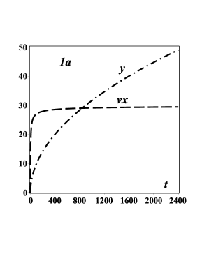
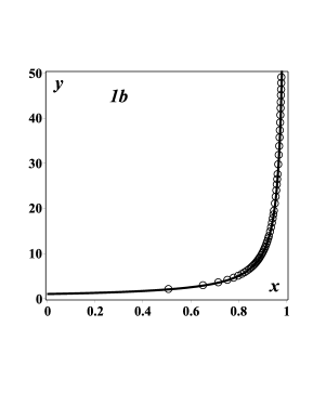
Figure 1: 1a — the dependences $x=x(t)$ and $y=y(t)$ obtained by numerical solution of the problem (17) for $a=b=1$ and $\gamma=2$ ($\nu=30$); 1b — exact solution (4) (solid line) and numerical solution of the problem (17) for $a=b=1$ and $\gamma=2$ (circles).

Remark 2.

Here and in what follows, the numerical integration interval for the new variable $t$ (or $\xi$) is usually determined, for demonstration calculations, from the condition $\Lambda_{\text{m}}=50$, where

$$\Lambda_{\text{m}}=\min[y,\,y^{\prime}_{x}/y]\quad\ \text{(for $y_{0}\sim 1$ and $y_{1}=y^{\prime}_{x}(x_{0})\sim 1$)}.$$ (19)

In a few cases, the condition $\Lambda_{\text{m}}=100$ or $\Lambda_{\text{m}}=150$ is used, which is specially stipulated. For first-order ODE problems of the form (10)–(11), this definition of $\Lambda_{\text{m}}$ can be replaced by the equivalent definition $\Lambda_{\text{m}}=\min[y,\,f/y]$.

Conditions $y_{0}\sim 1$ and $y_{1}\sim 1$ in (19) are not strongly essential, since the substitution $y=y_{0}-1+(y_{1}-1)(x-x_{0})+\bar{y}$ leads to an equivalent problem with the initial conditions $\bar{y}(x_{0})=\bar{y}^{\prime}_{x}(x_{0})=1$.

2.3 Modified differential transformation

The solution (18) tends rather slowly to the asymptotic values $x\to x_{*}$ as $t\to\infty$ (in particular, for $s=2$ and large $t$ we have $x_{*}-x\sim t^{-1/2}$). To speed up the process of approaching the asymptotic behavior with respect to $x$ in the system (14) is useful additionally to make the exponential-type substitution

$$t=t_{0}\exp(\lambda\tau),\quad\ \tau\geq 0,$$ (20)

where

$$\tau=\frac{\mskip 1.0mu1\mskip 1.0mu}{\mskip 1.0mu\lambda\mskip 1.0mu}\ln\frac{\mskip 1.0mut\mskip 1.0mu}{\mskip 1.0mut_{0}\mskip 1.0mu}=\frac{\mskip 1.0mu1\mskip 1.0mu}{\mskip 1.0mu\lambda\mskip 1.0mu}\ln\frac{\mskip 1.0muy^{\prime}_{x}\mskip 1.0mu}{\mskip 1.0mut_{0}\mskip 1.0mu}$$ (21)

is a new independent variable and $\lambda>0$ is a numerical parameter that can be varied. Transformations with a new independent variable of the form (21) will be called the modified differential transformations.

Example 4.

As a result of the substitution (20), the Cauchy problem (17) is transformed to the form

$$\begin{gathered}x^{\prime}_{\tau}=\frac{\mskip 1.0mu\lambda\mskip 1.0mu}{\mskip 1.0mub\gamma y^{\gamma-1}\mskip 1.0mu},\quad\ y^{\prime}_{\tau}=\frac{\mskip 1.0mua^{\gamma}\lambda e^{\lambda\tau}\mskip 1.0mu}{\mskip 1.0mu\gamma y^{\gamma-1}\mskip 1.0mu}\quad\ (\tau>0);\\ x(0)=0,\quad\ y(0)=a,\end{gathered}$$ (22)

and its exact solution is given by the formulas

$$x=\frac{\mskip 1.0mu1\mskip 1.0mu}{\mskip 1.0mua^{\gamma-1}b(\gamma-1)\mskip 1.0mu}\biggl{\{}1-\exp\biggl{[}-\frac{\mskip 1.0mu\lambda(\gamma-1)\mskip 1.0mu}{\mskip 1.0mu\gamma\mskip 1.0mu}\tau\biggr{]}\biggr{\}},\quad\ y=a\exp\biggl{(}\frac{\mskip 1.0mu\lambda\mskip 1.0mu}{\mskip 1.0mu\gamma\mskip 1.0mu}\tau\biggr{)},\qquad\tau\geq 0.$$ (23)

Let $a=b=1$, $\gamma=2$ and the stepsize is equal to $0.4$. For numerical integration of the test problem (22) for $\lambda=1$ and $\lambda=2$ with the maximum error $0.002\%$, it is required to take, respectively, the interval $[0,8]$ and $[0,4]$ with respect to $\tau$ to approach the asymptote (however, for numerical integration of the related problem (17) with the maximum error $0.016\%$, it is required to take an essentially larger interval $[0,2980]$ with respect to $t$).

3 Problems for first-order equations. Nonlocal transformations and
differential constraints

3.1 Solution method based on introducing a non-local variable

Introducing a new non-local variable [23, 24, 25] according to the formula,

$$\xi=\int^{x}_{x_{0}}g(x,y)\,dx,\quad\ y=y(x),$$ (24)

leads the Cauchy problem for one equation (10)–(11) to the equivalent problem for the autonomous system of equations

$$\begin{gathered}x^{\prime}_{\xi}=\frac{\mskip 1.0mu1\mskip 1.0mu}{\mskip 1.0mug(x,y)\mskip 1.0mu},\quad\ y^{\prime}_{\xi}=\frac{\mskip 1.0muf(x,y)\mskip 1.0mu}{\mskip 1.0mug(x,y)\mskip 1.0mu}\quad\ (\xi>0);\\ x(0)=x_{0},\quad\ y(0)=y_{0}.\qquad\qquad\end{gathered}$$ (25)

Here, the function $g=g(x,y)$ has to satisfy the following conditions:

$$g>0\ \text{for}\ x\geq x_{0},\ y\geq y_{0};\quad\ g\to\infty\ \text{as}\ y\to\infty;\quad\ f/g=k\ \text{as}\ y\to\infty,$$ (26)

where $k=\text{const}>0$ (moreover, the limiting case $k=\infty$ is also allowed); otherwise the function $g$ can be chosen rather arbitrarily.

From (24) and the second condition (26) it follows that $x^{\prime}_{\xi}\to 0$ as $\xi\to\infty$. The Cauchy problem (25) can be integrated numerically applying the Runge–Kutta method or other standard numerical methods.

Let us consider some possibilities for choosing the function $g=g(x,y)$ in the Cauchy problem (25) on concrete examples.

$1^{\circ}$. The special case

$$g=f$$

is equivalent to the hodograph transformation with an additional shift of the dependent variable, which gives $\xi=y-y_{0}$.

$2^{\circ}$. Setting

$$g=\sqrt{1+f^{2}},$$

we arrive at the method of the arc-length transformation [4]. In this case, the Cauchy problem (25) takes the form

$$\begin{gathered}x^{\prime}_{\xi}=\frac{\mskip 1.0mu1\mskip 1.0mu}{\mskip 1.0mu\sqrt{1+f^{2}(x,y)}\mskip 1.0mu},\quad\ y^{\prime}_{\xi}=\frac{\mskip 1.0muf(x,y)\mskip 1.0mu}{\mskip 1.0mu\sqrt{1+f^{2}(x,y)}\mskip 1.0mu};\\ x(0)=x_{0},\quad\ y(0)=y_{0}.\end{gathered}$$ (27)

$3^{\circ}$. Choosing

$$g=1+|f|,$$

we obtain the Cauchy problem

$$\begin{gathered}x^{\prime}_{\xi}=\frac{\mskip 1.0mu1\mskip 1.0mu}{\mskip 1.0mu1+|f(x,y)|\mskip 1.0mu},\quad\ y^{\prime}_{\xi}=\frac{\mskip 1.0muf(x,y)\mskip 1.0mu}{\mskip 1.0mu1+|f(x,y)|\mskip 1.0mu};\\ x(0)=x_{0},\quad\ y(0)=y_{0}.\end{gathered}$$ (28)

Note that we use here the absolute value sign to generalize the results, since the system (28) can also be used in the case $f<0$ for numerical integration of the problems having solutions with a root singularity [2].

$4^{\circ}$. We can also take the function

$$g=c_{1}+\bigl{(}c_{2}+|f|^{s}\bigr{)}^{1/s}$$

for $c_{1}\geq 0$, $c_{2}\geq 0$ ($|c_{1}|+|c_{2}|\not=0$), and $s>0$, which is a generalization of the functions in Items $2^{\circ}$ and $3^{\circ}$.

$5^{\circ}$. A very convenient problem for analysis can be obtained if we take

$$g=f/y$$ (29)

in (25). In this case, the second equation of the system is immediately integrated and, taking into account the initial condition, we get $y=y_{0}e^{\xi}$. In addition, the variable $x$ tends exponentially rapidly to a blow-up point $x_{*}$ with increasing $\xi$. This transformation will be called the special exp-type transformation.

Remark 3.

From Items $1^{\circ}$ and $2^{\circ}$ it follows that the method based on the hodograph transformation and the method of the arc-length transformation are particular cases of the method based on a non-local transformation of the general form (24).

Remark 4.

The functions $g$ in Items $1^{\circ}\hbox{--}4^{\circ}$ correspond to the value $k=1$ in (26), and the function $g$ in Item $5^{\circ}$ gives $k=\infty$.

Remark 5.

Nonlocal transformations of a special form were used in [25, 26, 27] to obtain exact solutions and to linearize some second-order ODEs.

3.2 Test problems and numerical solutions

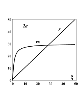
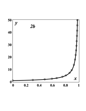
Figure 2: 2a  — the dependences $x=x(\xi)$ and $y=y(\xi)$, obtained by numerical solution of the problem (30) ($\nu=30$); 2b  — exact solution (4) (solid line) and numerical solution of the problem (30) (circles).

Example 5.

For the test Cauchy problem (3) with $f=y^{2}$, the equivalent problem for the system of equations (27) takes the form

$$\begin{gathered}x^{\prime}_{\xi}=\frac{\mskip 1.0mu1\mskip 1.0mu}{\mskip 1.0mu\sqrt{1+y^{4}}\mskip 1.0mu},\quad\ y^{\prime}_{\xi}=\frac{\mskip 1.0muy^{2}\mskip 1.0mu}{\mskip 1.0mu\sqrt{1+y^{4}}\mskip 1.0mu};\qquad x(0)=0,\quad\ y(0)=1.\end{gathered}$$ (30)

The second equation of this system is an equation with separable variables whose solution is not expressed in elementary functions.

The numerical solution of the Cauchy problem (30) in parametric form and its comparison with the exact solution (4) are shown in Fig. 2.

Example 6.

For the test Cauchy problem (3), the equivalent the problem for the system of equations (28) admits an exact solution, which is expressed in terms of elementary functions in a parametric form as follows:

$$\begin{gathered}x=1+{\textstyle\frac{\mskip 1.0mu1\mskip 1.0mu}{\mskip 1.0mu2\mskip 1.0mu}}\xi-{\textstyle\frac{\mskip 1.0mu1\mskip 1.0mu}{\mskip 1.0mu2\mskip 1.0mu}}\sqrt{\xi^{2}+4},\quad\ y={\textstyle\frac{\mskip 1.0mu1\mskip 1.0mu}{\mskip 1.0mu2\mskip 1.0mu}}\xi+{\textstyle\frac{\mskip 1.0mu1\mskip 1.0mu}{\mskip 1.0mu2\mskip 1.0mu}}\sqrt{\xi^{2}+4}\qquad(\xi\geq 0).\end{gathered}$$ (31)

This solution satisfies the initial conditions $x(0)=0$ and $y(0)=1$ and has no singularities. The function $x(\xi)$ is bounded, increases monotonically, and tends to its limiting value $\displaystyle x_{*}=\lim_{\xi\to\infty}x(\xi)=1$. The function $y(\xi)$ increases monotonically and tends to infinity as $\xi\to\infty$. At large $\xi$ we have $x\approx 1-\xi^{-1}$ and $y\approx\xi+\xi^{-1}$.

The curves $x=x(\xi)$ and $y=y(\xi)$, determined by the exact solution (31) (and also the curves obtained by numerical integration of the corresponding system (28) with $f=y^{2}$, $x_{0}=0$, and $y_{0}=1$), are very close to the curves shown in Fig. 2 (they almost merge with them and therefore are not presented here).

Example 7.

Consider the test problem (5)–(6), where $f=by^{\gamma}$, and take $g=f/y=by^{\gamma-1}$ (see Item $5^{\circ}$ in Section 3.1). Substituting these functions into (25), we obtain the Cauchy problem

$$\begin{gathered}x^{\prime}_{\xi}=\frac{\mskip 1.0mu1\mskip 1.0mu}{\mskip 1.0muby^{\gamma-1}\mskip 1.0mu},\quad\ y^{\prime}_{\xi}=y\quad\ (\xi>0);\\ x(0)=0,\quad y(0)=a,\end{gathered}$$ (32)

where $a>0$, $b>0$, and $\gamma>1$. The exact solution of the problem (32) is written as follows:

$$x=\frac{\mskip 1.0mu1\mskip 1.0mu}{\mskip 1.0mua^{\gamma-1}b(\gamma-1)\mskip 1.0mu}\bigl{[}1-e^{-(\gamma-1)\xi}\bigr{]},\quad\ y=ae^{\xi}.$$ (33)

It can be seen that the unknown function $x=x(\xi)$ tends exponentially to the asymptotic value $\displaystyle x_{*}=\frac{\mskip 1.0mu1\mskip 1.0mu}{\mskip 1.0mua^{\gamma-1}b(\gamma-1)\mskip 1.0mu}$ as $\xi\to\infty$.

Let $b=1$ and $\gamma=2$. The numerical solutions of the problems (17) and (32), obtained by the Runge–Kutta method of the fourth-order of approximation, are shown in Fig. 3 for $a=1$ and $a=2$ and the same step of integration, equal to $0.2$. We note that for this stepsize, the maximum difference between the exact solution (33) and the numerical solution of the system (32) is $0.0045\%$ (and for stepsize $0.4$, respectively, $0.061\%$).

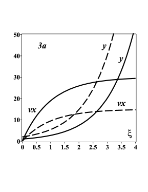
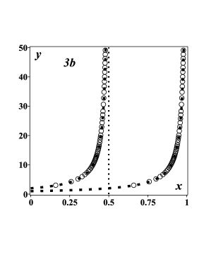
Figure 3: 3a  — the dependences $x=x(\xi)$ and $y=y(\xi)$, obtained by numerical solution of the problem (32) for $b=1$, $\gamma=2$ with $a=1$ (solid lines) and $a=2$ (dashed lines) ($\nu=30$); 3b  — numerical solution of the problem (17) for $b=1$, $\gamma=2$ (circles) and numerical solution of the problem (32) for $b=1$, $\gamma=2$ (points); for left curves $a=2$ and for right curves $a=1$.

It can be seen (see Figs. 1 and 3) that the numerical solutions are in a good agreement, but the rates of their approximation to the required asymptote $x=x_{*}$ are significantly different. For example, for the system (17), in order to obtain a good approximation to the asymptote, it is required to consider the interval $t\in[1,2980]$, and for the system (32) it suffices to take $\xi\in[0,4]$. Therefore, there is reason to believe that the method described in Item $5^{\circ}$ (a special case of the transformation (24)) is more efficient than the method based on the differential transformation (see Section 2.1).

For comparison, similar calculations were also performed applying the method based on the hodograph transformation (see Section 3.1, Item $1^{\circ}$), and the method of the arc-length transformation (see Section 3.1, Item $2^{\circ}$). For both of these methods, in order to obtain a good approximation to the asymptote, it is required to consider the interval $\xi\in[0,49]$. To control a numerical integration process, the calculations were carried out with the aid of the three most important and powerful mathematical software packages: Maple (2016), Mathematica (11), and MATLAB (2016a). It was found that the method based on the use of a special case of the system (25) with $g=f/y$ (see Item $5^{\circ}$) is essentially more efficient than the method based on the hodograph transformation and the method of the arc-length transformation.

Example 8.

We now consider the Cauchy problem (8) for $b=1$, which is determined by the exponential $f=e^{y}$. Substituting the function $g=f/y=e^{y}/y$ (see Item $5^{\circ}$ in Section 3.1) into the system (25), we obtain

$$\begin{gathered}x^{\prime}_{t}=ye^{-y},\quad\ y^{\prime}_{t}=y;\\ x(0)=0,\quad y(0)=a.\end{gathered}$$

The exact solution of this problem in a parametric form is defined by the formulas

$$x=e^{-a}-\exp(-a\,e^{t}),\quad\ y=ae^{t}\qquad(t\geq 0),$$

which do not have singularities. The function $x=x(t)$ is bounded, monotonically increases with increasing $t$ and very rapidly tends to the asymptote $\displaystyle x_{*}=\lim_{t\to\infty}x(t)=e^{-a}$, and the function $y=y(t)$ is unbounded and grows exponentially with respect to $t$.

3.3 Generalizations based on the use of differential constraints

Let us show that the method based on introducing a non-local variable (24) allows a further generalization.

We add to the equation (10) a first-order differential constraint [28] of the form

$$\xi^{\prime}_{x}=g(x,y,\xi)$$ (34)

and the initial condition $\xi(x=x_{0})=\xi_{0}$.

In a particular case, when the function $g$ does not depend on $\xi$, the use of the differential constraint (34), after integrating it over $x$, leads to the non-local variable (24) for $\xi_{0}=0$ (therefore, the method based on the differential constraint generalizes the method based on introducing a non-local variable).

From (10) and (34) we obtain the following system of ordinary differential equations:

$$x^{\prime}_{\xi}=\frac{\mskip 1.0mu1\mskip 1.0mu}{\mskip 1.0mug(x,y,\xi)\mskip 1.0mu},\quad\ y^{\prime}_{\xi}=\frac{\mskip 1.0muf(x,y)\mskip 1.0mu}{\mskip 1.0mug(x,y,\xi)\mskip 1.0mu}.$$ (35)

In a particular case,

$$g(x,y,\xi)=f_{x}+\xi f_{y},$$

the system (35) coincides with the system (16), in which the variable $t$ must be redenoted by $\xi$. If, in addition, we set $\xi_{0}=f(x_{0},y_{0})$, then, up to renaming of variables, we also obtain the initial conditions (15). It follows that the method based on the differential constraint of general form (34) generalizes the method based on introducing a differential variable (see Section 2.1).

3.4 Comparison of efficiency of various transformations for numerical integration of first-order ODE blow-up problems

In Table 1, a comparison of the efficiency of the numerical integration methods, based on various non-local transformations of the form (24) and differential constraints of the form (34) is presented by using the example of the test blow-up problem for the first-order ODE (3) with $f=y^{2}$. The comparison is based on the number of grid points needed to perform calculations with the same maximum error (approximately equal to $0.1$, $0.01$, and $0.005$). In the last line of Table 1 for Example 4 we take $a=b=1$ and $s=2$.

$\frac{\mskip 1.0mu1\mskip 1.0mu}{\mskip 1.0mu2\mskip 1.0mu}$ Error${}_{{\rm max}},\%=0.1$
Transformation or	Function $g$	Max. interval	Stepsize	Grid points
differential constraint	or Example	$\xi_{{\rm max}}\qquad$	$h\quad$	number $N$
Hodograph, Item $1^{\circ}$	$g{=}f$	48.99	0.2300	213
Arc-length, Item $2^{\circ}$	$g{=}\sqrt{1{+}f^{2}}$	49.20	0.3000	164
Nonlocal, Item $3^{\circ}$	$g{=}1{+}|f|$	50.00	0.4000	125
Special exp-type, Item $5^{\circ}$	$g{=}f/y$	3.925	0.1570	25
Diff. constraint	$g{=}f/[y(1+2\xi)]$	1.543	0.0643	24
Differential, modified	Example 4 with $\lambda=2$	3.910	0.2300	17
Error${}_{{\rm max}},\%=0.01$
Transformation or	Function $g$	Max. interval	Stepsize	Grid points
differential constraint	or Example	$\xi_{{\rm max}}\qquad$	$h\quad$	number $N$
Hodograph, Item $1^{\circ}$	$g{=}f$	49.01	0.130	377
Arc-length, Item $2^{\circ}$	$g{=}\sqrt{1{+}f^{2}}$	49.30	0.170	290
Nonlocal, Item $3^{\circ}$	$g{=}1{+}|f|$	50.14	0.230	218
Special exp-type, Item $5^{\circ}$	$g{=}f/y$	3.960	0.090	44
Diff. constraint	$g{=}f/[y(1+2\xi)]$	1.540	0.035	44
Differential, modified	Example 4 with $\lambda=2$	3.900	0.130	30
Error${}_{{\rm max}},\%=0.005$
Transformation or	Function $g$	Max. interval	Stepsize	Grid points
differential constraint	or Example	$\xi_{{\rm max}}\qquad$	$h\quad$	number $N$
Hodograph, Item $1^{\circ}$	$g{=}f$	49.035	0.1050	467
Arc-length, Item $2^{\circ}$	$g{=}\sqrt{1{+}f^{2}}$	49.266	0.1380	357
Nonlocal, Item $3^{\circ}$	$g{=}1{+}|f|$	50.135	0.1850	271
Special exp-type, Item $5^{\circ}$	$g{=}f/y$	3.9150	0.0725	54
Diff. constraint	$g{=}f/[y(1+2\xi)]$	1.5420	0.0291	53
Differential, modified	Example 4 with $\lambda=2$	3.9140	0.1030	38

Table 1: Various types of analytical transformations applied for numerical integration of the problem (3) for $f=y^{2}$ with a given accuracy (percent errors are $0.1$, $0.01$, and $0.005$ for $\Lambda_{\text{m}}\leq 50$) and their basic parameters (maximum interval, stepsize, grid points number).

It can be seen that for the first three transformations it is necessary to use a lot of grid points (the hodograph transformation is the least effective). This is due to the fact that in these cases $x$ tends to the point $x_{*}$ rather slowly for large $\xi$ ($x_{*}-x\sim 1/\xi$, $y\sim\xi$). The last three transformations require a significantly less number of grid points; in these cases $x$ tends exponentially fast to the point $x_{*}$ for large $\xi$. In particular, the use of the exp-type transformation with $g=t/y$ gives rather good results. The most effective analytical transformation is a modification of the method of differential transformations (see Example 4 in Section 2.3).

3.5 Complex blow-up problems, in which the right-hand side of the equation and the solution can change the sign

Up to now it has been assumed that the right-hand side of the equation (10) is positive. If we remove this restriction and assume that the function $f=f(x,y)$, and also the solution $y=y(x)$, can change sign for $x>x_{0}$ (in addition, $y_{0}$ can be any sign), then we can act in the following two stages:

(i) In the first stage, the problem (10)–(11) is integrated by applying a standard numerical method and the value $\Lambda_{m}=\min\{|y/y_{0}|,\ |y^{\prime}_{x}/y|\}$ (for $y_{0}\sim 1$) is calculated at the grid points $x_{m}$. When the value $\Lambda_{\text{m}}$ becomes sufficiently large (for example, $\Lambda_{\text{m}}=30$), then the calculation stops. The results of the integration performed are used in the region $x_{0}\leq x\leq x_{m}$.

(ii) In the second stage, we set the initial condition $y(x_{m})=y_{m}$ at the point $x_{m}$ to obtain a solution in the region $x>x_{m}$ (here $y_{m}$ is the value calculated on the first stage). Then a non-local transformation is applied (for example, described in Item $5^{\circ}$ in Section 3.1) and the resulting problem is integrated applying standard fixed-step numerical methods.

4 Problems for first-order equations, the right-hand side of which has
singularities or zeros

4.1 Blow-up problems for equations, the right-hand side of which has
singularities in $x$

In this section we will analyze several blow-up problems for equations of the form (10), the right-hand side of which has a singularity at some $x=x_{\text{s}}$, i.e. $\displaystyle\lim_{x\to x_{\text{s}}}f(x,y)=\infty$.

We assume that the right-hand side of equation (10) can be represented as a product of two functions

$$f(x,y)=f_{\text{b}}(x,y)f_{\text{s}}(x,y),$$ (36)

where the function $f_{\text{b}}$ has the same properties as the function $f$ in Section 2.1 (i.e. that the problem (10)–(11), where the function $f$ is replaced by $f_{\text{b}}$, has a blow-up solution).

Moreover, we will assume that the function $f_{\text{s}}$ has an integrable or non-integrable singularity at $x=x_{\text{s}}$, so that $\displaystyle\lim_{x\to x_{\text{s}}}f(x,y)=\infty$, and $f_{\text{s}}>0$ at $x_{0}<x_{\text{s}}$.

It is interesting to see how the two singularities of this problem will interact: the blow-up singularity and the coordinate singularity at $x=x_{\text{s}}$.

For the sake of clarity, we give the following test problems and illustrative examples.

Example 9.

Consider the two-parameter test Cauchy problem:

$$y^{\prime}_{x}=\frac{\mskip 1.0muy^{2}\mskip 1.0mu}{\mskip 1.0mub-x\mskip 1.0mu};\quad\ y(0)=a,$$ (37)

where $a>0$ and $b>0$. For this problem, we have $f_{\text{b}}=y^{2}$ and $f_{\text{s}}=1/(b-x)$. The right-hand side of equation (37) has a pole of the first order at the point $x=x_{\text{s}}=b$ (i.e., there exists a non-integrable singularity at this point); and the right-hand side of the equation becomes negative if $x>b$.

The exact solution of the problem (37) has the form

$$y=\biggl{[}\ln\Bigl{(}1-\frac{\mskip 1.0mux\mskip 1.0mu}{\mskip 1.0mub\mskip 1.0mu}\Bigr{)}+\frac{\mskip 1.0mu1\mskip 1.0mu}{\mskip 1.0mua\mskip 1.0mu}\biggr{]}^{-1}.$$ (38)

The singular point of this solution is determined by the formula

$$x_{*}=b\bigl{(}1-e^{-1/a}\bigr{)}<b.$$ (39)

Here the blow-up singularity “overtakes” the non-integrable singularity of the equation at the point $x_{\text{s}}=b$. If $a\to\infty$, we have $x_{*}\to b$.

Example 10.

Consider the test Cauchy problem with a stronger coordinate singularity:

$$y^{\prime}_{x}=\frac{\mskip 1.0muy^{2}\mskip 1.0mu}{\mskip 1.0mu(b-x)^{2}\mskip 1.0mu};\quad\ y(0)=a,$$ (40)

where $a>0$ and $b>0$. For this problem, we have $f_{\text{b}}=y^{2}$ and $f_{\text{s}}=1/(b-x)^{2}$. The right-hand side of equation (40) has a pole of the second order at the point $x_{\text{s}}=b$ (i.e., there exists a non-integrable singularity at this point); and right-hand side of this equation is positive for all $x$.

The exact solution of the problem (40) is defined by the formula

$$y=\frac{\mskip 1.0muab\mskip 1.0mu}{\mskip 1.0mua+b\mskip 1.0mu}\biggl{[}1+\frac{\mskip 1.0muab\mskip 1.0mu}{\mskip 1.0mub^{2}-(a+b)x\mskip 1.0mu}\biggr{]}.$$ (41)

The blow-up point is determined as

$$x_{*}=\frac{\mskip 1.0mub^{2}\mskip 1.0mu}{\mskip 1.0mua+b\mskip 1.0mu}<b.$$ (42)

Here, as in Example 9, the blow-up singularity “overtakes” the non-integrable singularity of the equation at the point $x_{\text{s}}=b$.

Remark 6.

A qualitatively similar picture will occur also for the problem (10)–(11) with $f=y^{2}/\sqrt{b-x}$, which has an integrable singularity at the point $x=b$. In this problem, the right-hand side of the equation is defined only on a part of the $x$-axis.

The solution property, described in Examples 9 and 10, has a general characteristic. Namely, let us assume that the right-hand side of equation (10) has the form (36), where the functions $f_{\text{b}}$ and $f_{\text{s}}$ have the properties described at the beginning of this section. Then the problem (10)–(11) has a blow-up solution, and the domain of definition of this solution is located to the left of the point $x_{\text{s}}$ (i.e., $x_{*}<x_{\text{s}}$, where $x_{*}$ is the blow-up point).

The methods described in Sections 2 and 3 can be applied for solving this type of problems with the coordinate singularity.

Example 11.

For test problem (37) with $f=y^{2}/(b-x)$, we take (see Item $5^{\circ}$ in Section 3.1),

$$g=\frac{\mskip 1.0muf\mskip 1.0mu}{\mskip 1.0muy\mskip 1.0mu}=\frac{\mskip 1.0muy\mskip 1.0mu}{\mskip 1.0mub-x\mskip 1.0mu}.$$

By substituting these functions in (25), we arrive at the Cauchy problem for a system of coupled ODEs

$$\begin{gathered}x^{\prime}_{\xi}=\frac{\mskip 1.0mub-x\mskip 1.0mu}{\mskip 1.0muy\mskip 1.0mu},\quad\ y^{\prime}_{\xi}=y\quad\ \ (\xi>0);\\ x(0)=0,\quad y(0)=a.\end{gathered}$$ (43)

The exact solution of this problem reads

$$x=b\biggl{\{}1-\exp\biggl{[}-\frac{\mskip 1.0mu1\mskip 1.0mu}{\mskip 1.0mua\mskip 1.0mu}(1-e^{-\xi})\biggr{]}\biggr{\}},\quad\ y=ae^{\xi}.$$ (44)

The numerical solution of the problem (43) with $a=b=1$ is presented in Fig. 4a; the dependences $x=x(\xi)$ and $y=y(\xi)$ are obtained by the fourth-order Runge–Kutta method. Fig. 4b shows a comparison of the exact solution (38) of the Cauchy problem (37) for one equation with the numerical solution of the problem for the system of two equations (43).

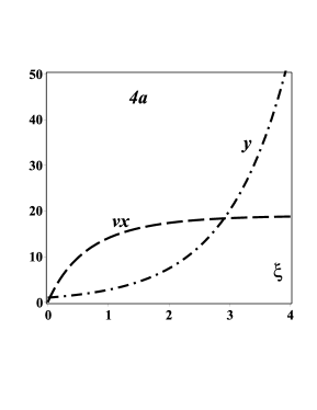
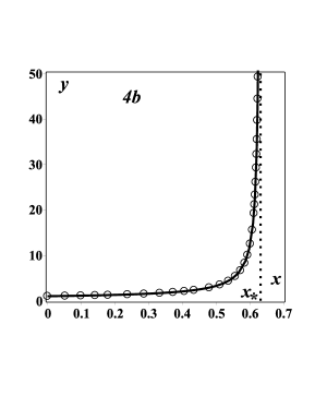
Figure 4: 4a — numerical solutions of system (43), the dependences $x=x(\xi)$ and $y=y(\xi)$ (where $\nu=30$); 4b — exact solution (38), solid line, and the numerical solution of system (43) ($a=b=1$ and $x_{*}=0.6321$).

Remark 7.

A form of the right-hand side of equation (10) with a coordinate singularity at the point $x_{\text{s}}$ can mislead the researcher, inexperienced in blow-up problems. As a result, the researcher will start to refine a mesh (making it thinner) in the neighborhood of the point $x_{\text{s}}$ (what should not to do).

4.2 Blow-up problems for equations, the right-hand side of which has zeros

In this section we will analyze blow-up problems for equations of the form (10), the right-hand side of which vanishes at some $x=x_{\text{z}}$, i.e. $f(x_{\text{z}},y)=0$.

Let us assume that the right-hand side of equation (10) can be represented as a product of two functions

$$f(x,y)=f_{\text{b}}(x,y)f_{\text{z}}(x,y),$$ (45)

where the function $f_{\text{b}}$ has the same properties as the function $f$ in Section 2.1 (i.e., the problem (10)–(11), where the function $f$ is replaced by $f_{\text{b}}$, has a blow-up solution). Moreover, we will assume that the function $f_{\text{z}}$ vanishes at $x=x_{\text{z}}$, so that $f(x_{\text{z}},y)=0$, and $f_{\text{z}}>0$ at $x_{0}<x_{\text{z}}$.

Example 12.

Consider the test two-parameter Cauchy problem

$$y^{\prime}_{x}=y^{2}(b-x);\quad\ y(0)=a,$$ (46)

where $a>0$ and $b>0$. For this problem, we have $f_{\text{b}}=y^{2}$ and $f_{\text{z}}=b-x$. The right-hand side of equation (46) becomes zero at the point $x=x_{\text{z}}=b$; and the right-hand side of the equation becomes negative if $x>b$.

It is interesting to see how two features of different types of such problem will interact: on the one hand, a possible blow-up singularity (which leads to an unlimited growth of the right-hand side of the equation), and on the other hand, vanishing of the right-hand side of the equation at $x=x_{\text{z}}$.

The exact solution of the problem (46) has the form

$$y=\frac{\mskip 1.0mua\mskip 1.0mu}{\mskip 1.0mu\frac{\mskip 1.0mu1\mskip 1.0mu}{\mskip 1.0mu2\mskip 1.0mu}ax^{2}-abx+1\mskip 1.0mu}.$$ (47)

The existence or absence of a blow-up singularity in this solution is determined by the existence or absence of real roots of the quadratic equation $\frac{\mskip 1.0mu1\mskip 1.0mu}{\mskip 1.0mu2\mskip 1.0mu}ax^{2}{-}abx{+}1{=}0$.

The elemental analysis shows that there are two qualitatively different cases:

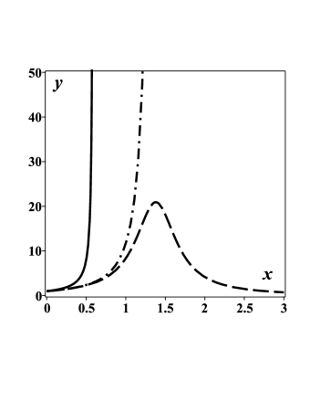
Figure 5: Exact solutions (47) of the Cauchy problem (46) for various values of the parameters: $a=1$, $b=1.38$ (dashed line); $a=1$, $b=2$ (solid line); and $a=1$, $b=\sqrt{2}$ (dashed-dot line).

(i) If $0<b<\sqrt{2/a}$, there exists a smooth continuous solution of the problem for all $x\geq 0$. It is monotonically increasing on the interval $0\leq x<b$, reaches the maximum value $\displaystyle y_{m}=\frac{\mskip 1.0mua\mskip 1.0mu}{\mskip 1.0mu1-\frac{\mskip 1.0mu1\mskip 1.0mu}{\mskip 1.0mu2\mskip 1.0mu}ab^{2}\mskip 1.0mu}$, and decreases for $x>b$.

(ii) If $b\geq\sqrt{2/a}$, formula (47) defines a monotonically increasing blow-up solution with the singular point

$$x_{*}=b-\sqrt{b^{2}-\frac{\mskip 1.0mu2\mskip 1.0mu}{\mskip 1.0mua\mskip 1.0mu}}.$$ (48)

Therefore in this example the existence or absence of a blow-up solution is determined by a simple relation between the parameters $a$ and $b$: if $b\geq\sqrt{2/a}$, then there exists a blow-up solution, otherwise there is no a blow-up solution. The value $b=\sqrt{2/a}$ is a point of bifurcation of the two-parameter problem (46).

The exact solutions of the problem (46) obtained by formula (47) are presented in Fig. 5 for various values of the parameters: $a=1$ and $b=1$, $b=2$, and $b=\sqrt{2}$ (the critical value at which there exists blow-up solutions).

Similar problems are complicated for numerical integration in a wide range of changing of the parameters $a$ and $b$. First, it is reasonable to produce a direct integration of the problem (46) by the Runge–Kutta methods for specific values of $a$ and $b$. If a rapid growth of the solution occurs, then the methods described in Sections 2 or 3 should be applied (see also Section 3.4).

More efficient methods allowing to integrate numerically similar and more complex non-monotonic blow-up problems will be described in subsequent publications.

Remark 8.

A formal replacing $b-x$ to $(b-x)^{2}$ in the problem (46) leads to a blow-up solution for any $a>0$ and $b>0$.

5 Problems for first-order equations. Two-sided estimates of
the critical value

5.1 Autonomous equations. Analytical formula for the critical value

We consider the Cauchy problem for an autonomous equation of the general form

$$y^{\prime}_{x}=f(y)\quad(x>0),\quad\ y(0)=a.$$ (49)

We assume that $a>0$ and $f(y)>0$ is a continuous function that is defined for all $y\geq a$. An exact solution of the Cauchy problem (49) for $x>0$ can be represented implicitly as follows:

$$x=\int^{y}_{a}\frac{\mskip 1.0mud\xi\mskip 1.0mu}{\mskip 1.0muf(\xi)\mskip 1.0mu}.$$ (50)

This solution is a blow-up solution if and only if there exists a finite definite integral in (50) for $y=\infty$. In this case, the critical value $x_{*}$ is calculated as follows:

$$x_{*}=\int^{\infty}_{a}\frac{\mskip 1.0mud\xi\mskip 1.0mu}{\mskip 1.0muf(\xi)\mskip 1.0mu}.$$ (51)

Let the conditions formulated after the problem (49) be satisfied.

A necessary criterion for the existence of a blow-up solution is:

$$\lim_{y\to\infty}\frac{\mskip 1.0muf(y)\mskip 1.0mu}{\mskip 1.0muy\mskip 1.0mu}=\infty.$$

Sufficient criterion of the existence of a blow-up solution. Let the conditions formulated above are also satisfied and the limiting ratio,

$$\lim_{y\to\infty}\frac{\mskip 1.0muf(y)\mskip 1.0mu}{\mskip 1.0muy^{1+\kappa}\mskip 1.0mu}=s,\quad\ 0<s\leq\infty,$$ (52)

takes place for some parameter $\kappa>0$. Then the solution of the Cauchy problem (49) is a blow-up solution.

If $f(y)$ is a differentiable function, then instead of (52) we can propose an equivalent sufficient criterion of the existence of a blow-up solution:

$$\lim_{y\to\infty}\frac{\mskip 1.0muf^{\prime}_{y}(y)\mskip 1.0mu}{\mskip 1.0muy^{\kappa}\mskip 1.0mu}=s_{1},\quad\ 0<s_{1}\leq\infty\qquad(\kappa>0).$$

5.2 Non-autonomous equations. One-sided estimates

We consider the Cauchy problem for a first-order non-autonomous equation of the general form

$$y^{\prime}_{x}=f(x,y)\quad(x>0),\quad\ y(0)=a.$$ (53)

We assume that $f(x,y)$ is a continuous function and the conditions

$$f(x,y)\geq g(y)>0\quad\text{for all}\quad y\geq a>0,\quad\ \ x\geq 0$$ (54)

are satisfied. We also assume that there exists a finite integral

$$I_{g}=\int^{\infty}_{a}\frac{\mskip 1.0mud\xi\mskip 1.0mu}{\mskip 1.0mug(\xi)\mskip 1.0mu}<\infty.$$ (55)

Then the solution $y=y(x)$ of the Cauchy problem (53) is a blow-up solution, and the critical value $x_{*}$ satisfies the inequality

$$x_{*}\leq I_{g}.$$ (56)

This estimate follows from the inequality (see, for example, the corresponding comparison theorems in [29, 30]):

$$y(x)\geq y_{g}(x),$$ (57)

where $y(x)$ is the solution of the Cauchy problem (53), and $y_{g}(x)$ is the solution of the auxiliary Cauchy problem

$$y^{\prime}_{x}=g(y)\quad\ (x>0),\quad\ y(0)=a.$$ (58)

Example 13.

We consider the Cauchy problem for the Abel equation of the first kind

$$y^{\prime}_{x}=y^{3}+h(x)\quad(x>0);\quad\ y(0)=1.$$ (59)

If $h(x)\geq 0$ for $x\geq 0$, then the inequality is valid

$$f(x,y)\equiv y^{3}+h(x)\geq g(y)\equiv y^{3}>0\quad\text{for all}\quad y>1.$$

Calculating the integral (55) with $g(y)=y^{3}$, we obtain

$$I_{g}=\int^{\infty}_{1}\frac{\mskip 1.0mud\xi\mskip 1.0mu}{\mskip 1.0mu\xi^{3}\mskip 1.0mu}=\frac{\mskip 1.0mu1\mskip 1.0mu}{\mskip 1.0mu2\mskip 1.0mu}<\infty.$$ (60)

Therefore, the solution of the Cauchy problem (59) for $h(x)\geq 0$ is a blow-up solution, and $x_{*}\leq\frac{\mskip 1.0mu1\mskip 1.0mu}{\mskip 1.0mu2\mskip 1.0mu}$.

5.3 Non-autonomous equations. Two-sided estimates

We consider two cases in which the one-sided estimate (56) can be improved. We introduce the notations

$$I_{1}=\int^{\infty}_{y_{0}}\frac{\mskip 1.0mud\xi\mskip 1.0mu}{\mskip 1.0muf(0,\xi)\mskip 1.0mu},\quad\ I_{2}=\int^{\infty}_{y_{0}}\frac{\mskip 1.0mud\xi\mskip 1.0mu}{\mskip 1.0muf(I_{1},\xi)\mskip 1.0mu}.$$ (61)

Case $1^{\circ}$. Let $f_{x}\geq 0$. Suppose that the integral $I_{1}$ in (61) exists and is finite. Suppose also that the conditions,

$$f(x,y)>0,\quad f_{x}(x,y)\geq 0\quad\text{for all}\quad 0\leq x\leq I_{1},\ \ y\geq y_{0}>0,$$ (62)

are satisfied. Then the integral $I_{2}$ exists and the inequalities are valid:

$$f(0,y)\leq f(x,y)\leq f(I_{1},y)\quad\text{for}\quad 0\leq x\leq I_{1}$$ (63)

and

$$y_{1}(x)\leq y(x)\leq y_{2}(x)\quad\text{for}\quad 0\leq x\leq I_{2}\leq I_{1}.$$ (64)

Here $y(x)$ is the solution of the Cauchy problem (53), and $y_{1}(x)$ and $y_{2}(x)$ are the solutions of the corresponding auxiliary Cauchy problems:

$$y^{\prime}_{x} =f(0,y)\quad\ \ (x>0),\quad\ y(0)=y_{0};$$ (65)

$$y^{\prime}_{x} =f(I_{1},y)\quad\ (x>0),\quad\ y(0)=y_{0}.$$ (66)

The solutions $y_{1}(x)$ and $y_{2}(x)$ can be represented implicitly as follows:

$$x=\int^{y}_{y_{0}}\frac{\mskip 1.0mud\xi\mskip 1.0mu}{\mskip 1.0muf(0,\xi)\mskip 1.0mu},\quad\ x=\int^{y}_{y_{0}}\frac{\mskip 1.0mud\xi\mskip 1.0mu}{\mskip 1.0muf(I_{1},\xi)\mskip 1.0mu}.$$ (67)

For the critical value $x_{*}$, the two-sided estimate

$$I_{2}\leq x_{*}\leq I_{1}$$ (68)

is valid.

Case $2^{\circ}$. Let $f_{x}\leq 0$. Suppose that the integrals $I_{1}$ and $I_{2}$ in (61) exist and are finite. Suppose also that the conditions,

$$f(x,y)>0,\quad f_{x}(x,y)\leq 0\quad\text{for all}\quad 0\leq x\leq I_{2},\ \ y\geq y_{0}>0,$$ (69)

are satisfied. Then the following inequalities are valid:

$$f(I_{1},y)\leq f(x,y)\leq f(0,y)\quad\text{for}\quad 0\leq x\leq I_{2}$$ (70)

and

$$y_{2}(x)\leq y(x)\leq y_{1}(x)\quad\text{for}\quad 0\leq x\leq I_{1}\leq I_{2},$$ (71)

where $y(x)$ is the solution of the Cauchy problem (53), and $y_{1}(x)$ and $y_{2}(x)$ are the solutions of the corresponding auxiliary Cauchy problems (65) and (66). The last two solutions can be represented implicitly (67). For the critical value $x_{*}$, the two-sided estimate

$$I_{1}\leq x_{*}\leq I_{2}$$ (72)

is valid.

Example 14.

We consider the Cauchy problem for the Riccati equation

$$y^{\prime}_{x}=y^{2}+h(x)\quad(x>0);\quad\ y(0)=a>0.$$ (73)

Let us consider the two cases.

Case $1^{\circ}$. Let $h(x)\geq 0$ and $h^{\prime}_{x}(x)\geq 0$. In this case, the first auxiliary Cauchy problem (65) is written as follows:

$$y^{\prime}_{x}=y^{2}+h(0)\quad\ (x>0),\quad\ y(0)=a.$$ (74)

The exact solution of the problem (74) admits an implicit form of representation with the help of the first relation (67) for $y_{0}=a$ and $f(0,y)=y^{2}+h(0)$. After elementary calculations and transformations, this solution can be written in the explicit form

$$y=\sqrt{b}\,\frac{\mskip 1.0mua\cos(\sqrt{b}\,x)+\sqrt{b}\sin(\sqrt{b}\,x)\mskip 1.0mu}{\mskip 1.0mu\sqrt{b}\cos(\sqrt{b}\,x)-a\sin(\sqrt{b}\,x)\mskip 1.0mu},\quad\ b=h(0).$$ (75)

The singular point of this solution, $I_{1}$, which is the zero of the denominator and is equal to the improper first integral in (61) for $y_{0}=a$ and $f(0,y)=y^{2}+h(0)$, is defined by the formula

$$I_{1}=\frac{\mskip 1.0mu1\mskip 1.0mu}{\mskip 1.0mu\sqrt{b}\mskip 1.0mu}\arctan\frac{\mskip 1.0mu\sqrt{b}\mskip 1.0mu}{\mskip 1.0mua\mskip 1.0mu},\quad\ b=h(0).$$

The solution of the second auxiliary Cauchy problem (66) is given by the formula (75), in which $h(0)$ must be replaced by $h(I_{1})$. As a result, we obtain the two-sided estimate of the critical value $x_{*}$:

$$\begin{gathered}I_{2}\leq x_{*}\leq I_{1},\\ I_{1}=\frac{\mskip 1.0mu1\mskip 1.0mu}{\mskip 1.0mu\sqrt{h(0)}\mskip 1.0mu}\arctan\frac{\mskip 1.0mu\sqrt{h(0)}\mskip 1.0mu}{\mskip 1.0mua\mskip 1.0mu},\quad I_{2}=\frac{\mskip 1.0mu1\mskip 1.0mu}{\mskip 1.0mu\sqrt{h(I_{1})}\mskip 1.0mu}\arctan\frac{\mskip 1.0mu\sqrt{h(I_{1})}\mskip 1.0mu}{\mskip 1.0mua\mskip 1.0mu}.\end{gathered}$$ (76)

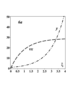
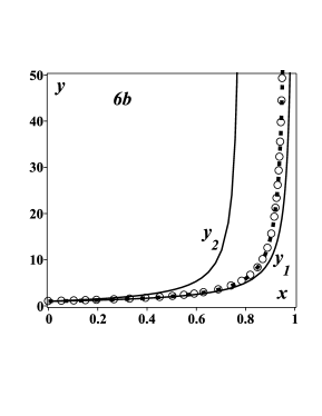
Figure 6: 6a — the dependences $x=x(\xi)$ and $y=y(\xi)$ obtained numerically after the transformation of the Cauchy problem for one equation (73) for $a=1$, $h(x)=x^{2}$ to the problem for the system of equations (25) for $f=y^{2}+x^{2}$, $g=f/y$ ($\nu=30$); 6b — the exact solution of the problem (73) (points), the numerical solution of this problem (circles), and the majorizing functions $y_{1}(x)$ and $y_{2}(x)$ (solid lines).

In particular, setting $a=1$, $h(x)=x^{m}$ and $m>0$ in (73), we find that $I_{1}=1$ and $I_{2}=\arctan 1$. Substituting these values into (76), we obtain the two-sided estimate $0.785\leq x_{*}\leq 1$ for the critical value $x_{*}$.

In Fig. 6 we present the results of the numerical solution of the Cauchy problem (73) for $a=1$ and $h(x)=x^{2}$ in parametric form, as well as a comparison of the numerical and exact solutions of this problem (the latter is expressed in terms of the Bessel functions and is omitted here), and also the majorizing functions $y_{1}=1/(1-x)$ and $y_{2}=y_{2}(x)$, which are the solutions of the auxiliary Cauchy problems (65) and (66) (the solution of the Cauchy problem under consideration is located between these functions). The function $y_{2}(x)$ is determined by the formula (75), in which the parameter $b$ must be replaced by $1/a$.

We note that if $h(x)=\text{const}>0$, then the inequalities (76) give the exact result $x_{*}=I_{1}=I_{2}$.

Case $2^{\circ}$. Let $h(x)\geq 0$ and $h^{\prime}_{x}(x)\leq 0$. In this case, the solution of the first auxiliary Cauchy problem (74) is also given by the formula (75), and the solution of the second auxiliary Cauchy problem is obtained from (75) by a formal replacement of $h(0)$ by $h(I_{1})$. As a result, we obtain the two-sided estimate for the critical value $x_{*}$:

$$I_{1}\leq x_{*}\leq I_{2},$$

where the integrals $I_{1}$ and $I_{2}$ are determined by the formulas (76).

Remark 9.

It should be noted that in Case $2^{\circ}$ it does not matter how the function $f(x,y)$ and its derivative $f_{x}(x,y)$ behave for $x>I_{2}$; in particular, the right-hand side of the equation (53) can be negative for $x>I_{2}$.

Example 15.

To illustrate what was said in Remark 9, we consider the test Cauchy problem

$$y^{\prime}_{x}=(2-x)y^{2}\quad(x>0);\quad\ y(0)=1,$$ (77)

which corresponds to Case $2^{\circ}$, where $f(x,y)<0$ for $x>2$.

Calculating the integrals (61), we have $I_{1}=\frac{\mskip 1.0mu1\mskip 1.0mu}{\mskip 1.0mu2\mskip 1.0mu}$ and $I_{2}=\frac{\mskip 1.0mu2\mskip 1.0mu}{\mskip 1.0mu3\mskip 1.0mu}$. Substituting these values into (72), we obtain the two-sided estimate for the singular point

$${\textstyle\frac{\mskip 1.0mu1\mskip 1.0mu}{\mskip 1.0mu2\mskip 1.0mu}}<x_{*}<{\textstyle\frac{\mskip 1.0mu2\mskip 1.0mu}{\mskip 1.0mu3\mskip 1.0mu}}.$$

The exact solution of the problem (77) is given by the formula

$$y=\frac{\mskip 1.0mu2\mskip 1.0mu}{\mskip 1.0mux^{2}-4x+2\mskip 1.0mu}.$$ (78)

The zero of the denominator, equal to $x_{*}=2-\sqrt{2}\approx 0.5858$, determines the singular point of the solution (first-order pole).

6 Problems for second-order equations. Differential transformations

6.1 Solution method based on introducing a differential variable

The Cauchy problem for the second-order differential equation has the form

$$y^{\prime\prime}_{xx}=f(x,y,y^{\prime}_{x})\quad(x>x_{0});$$ (79)

$$y(x_{0})=y_{0},\quad\ y^{\prime}_{x}(x_{0})=y_{1}.$$ (80)

We note that the exact solutions of equations of the form (79), which can be used for the formulation of test problems with blow-up solutions, can be found in [31, 32, 30, 33].

Let $f(x,y,u)>0$ if $y>y_{0}\geq 0$ and $u>y_{1}\geq 0$, and the function $f$ increases quite rapidly as $y\to\infty$ (for example, if $f$ does not depend on $y^{\prime}_{x}$, then $\displaystyle\lim_{y\to\infty}f/y=\infty$).

First, as in Section 2.1, we represent the ODE (79) as an equivalent system of differential-algebraic equations

$$y^{\prime}_{x}=t,\quad\ y^{\prime\prime}_{xx}=f(x,y,t),$$ (81)

where $y=y(x)$ and $t=t(x)$ are the unknown functions.

Taking into account (81), we derive a standard system of ODEs for the functions $y=y(t)$ and $x=x(t)$. To do this, differentiating the first equation of the system (81) with respect to $t$, we obtain $(y^{\prime}_{x})^{\prime}_{t}=1$.

Taking into account the relations $y^{\prime}_{t}=tx^{\prime}_{t}$ (it follows from the first equation (81)) and $(y^{\prime}_{x})^{\prime}_{t}=y^{\prime\prime}_{xx}/t^{\prime}_{x}=x^{\prime}_{t}y^{\prime\prime}_{xx}$, we have

$$x^{\prime}_{t}y^{\prime\prime}_{xx}=1.$$ (82)

Eliminating here the second derivative $y^{\prime\prime}_{xx}$ by using the second equation (81), we arrive at the first-order equation

$$x^{\prime}_{t}=\frac{\mskip 1.0mu1\mskip 1.0mu}{\mskip 1.0muf(x,y,t)\mskip 1.0mu}.$$ (83)

Considering further the relation $y^{\prime}_{t}=tx^{\prime}_{t}$, we transform (83) to the form

$$y^{\prime}_{t}=\frac{\mskip 1.0mut\mskip 1.0mu}{\mskip 1.0muf(x,y,t)\mskip 1.0mu}.$$ (84)

Equations (83) and (84) represent a system of coupled first-order differential equations for the unknown functions $x=x(t)$ and $y=y(t)$. The system (83)–(84) should be supplemented by the initial conditions

$$x(t_{0})=x_{0},\quad y(t_{0})=y_{0},\quad t_{0}=y_{1},$$ (85)

which are derived from (80) and the first equation (81).

The Cauchy problem (83)–(85) has a solution without blow-up singularities and can be integrated by applying the standard fixed-step numerical methods (see, for example, [14, 15, 16, 17, 18, 19, 20, 21, 22]).

Remark 10.

Systems of differential-algebraic equations (12) and (81) are particular cases of parametrically defined nonlinear differential equations, which are considered in [34, 35]. In [35], the general solutions of several parametrically defined ODEs were constructed via differential transformations based on introducing a new differential independent variable $t=y^{\prime}_{x}$.

6.2 Test problems and numerical solutions

Example 16.

We consider a test Cauchy problem for the second-order nonlinear ODE

$$y^{\prime\prime}_{xx} =b\gamma y^{\gamma-1}y^{\prime}_{x}\quad\ \ (x>0);\quad y(0)=a,\quad y^{\prime}_{x}(0)=a^{\gamma}b,$$ (86)

which is obtained by differentiating equation (5). For $a>0$, $b>0$, and $\gamma>1$, the exact solution of this problem is defined by the formula (7).

Introducing a new variable $t=y^{\prime}_{x}$ in (86), we obtain the Cauchy problem, which exactly coincides with the problem (17). The exact solution of this problem is determined by the formulas (18).

Example 17.

Let us now consider another Cauchy problem

$$y^{\prime\prime}_{xx} =b^{2}\gamma y^{2\gamma-1}\quad\ \ (x>0);\quad y(0)=a,\quad y^{\prime}_{x}(0)=a^{\gamma}b,$$ (87)

which is obtained by excluding the first derivative from the equations (5) and (86) (we recall that the second equation is a consequence of the first equation). The exact solution of the problem (87) is determined by the formula (7).

Introducing a new variable $t=y^{\prime}_{x}$, we transform (87) to the Cauchy problem for the system of the first-order ODEs

$$\begin{gathered}x^{\prime}_{t}=\frac{\mskip 1.0mu1\mskip 1.0mu}{\mskip 1.0mub^{2}\gamma y^{2\gamma-1}\mskip 1.0mu},\quad\ y^{\prime}_{t}=\frac{\mskip 1.0mut\mskip 1.0mu}{\mskip 1.0mub^{2}\gamma y^{2\gamma-1}\mskip 1.0mu}\quad\ (t>t_{0});\\ x(t_{0})=0,\quad y(t_{0})=a,\quad t_{0}=a^{\gamma}b,\end{gathered}$$ (88)

which is a particular case of the problem (83)–(85) with $f=b^{2}\gamma y^{2\gamma-1}$, $x_{0}=0$, and $y_{0}=a$. The exact solution of the problem (88) is given by formulas (18).

Figure 7 shows a comparison of the exact solution (4) of the Cauchy problem for one equation (3) with the numerical solution of the related problem for the system of equations (88) for $a=b=1$ and $\gamma=2$, obtained by applying the Runge–Kutta method of the fourth-order of approximation.

The function $x(t)$ slowly tends to the asymptotic value $x_{*}$. Therefore to accelerate this process in the system (88) is useful additionally to make the exponential-type substitution (20).

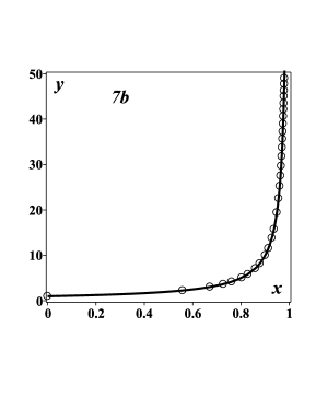
Figure 7: 7a — the dependences $x=x(t)$ and $y=y(t)$ obtained by numerical solution of the problem (88) for $a=b=1$ and $\gamma=2$ ($\nu=30$); 7b — exact solution (4) (solid line) and numerical solution of problem (88) (circles).

For completeness of the picture, we also give an example of a blow-up problem whose solution has a logarithmic singularity.

Example 18.

An exact solution of the Cauchy problem with exponential nonlinearity

$$y^{\prime\prime}_{xx}=e^{2y}\quad(x>0);\qquad y(0)=0,\quad y^{\prime}_{x}(0)=1,$$ (89)

has the form

$$y=\ln\Bigl{(}\frac{\mskip 1.0mu1\mskip 1.0mu}{\mskip 1.0mu1-x\mskip 1.0mu}\Bigr{)}=-\ln(1-x).$$ (90)

This solution has a logarithmic singularity at the point $x_{*}=1$ and does not exist for $x>x_{*}$.

Introducing the differential variable $t=y^{\prime}_{x}$, we transform the problem (89) to the following Cauchy problem for a system of equations:

$$\begin{gathered}x^{\prime}_{t}=e^{-2y},\quad\ y^{\prime}_{t}=te^{-2y}\quad\ (t>1);\\ x(1)=0,\quad\ y(1)=0\quad\ (t_{0}=1),\end{gathered}$$ (91)

which is a particular case of the system (83)–(84). The exact analytical solution of the problem (91) is determined by the formulas

$$x=1-\frac{\mskip 1.0mu1\mskip 1.0mu}{\mskip 1.0mut\mskip 1.0mu},\quad\ y=\ln t\qquad(t\geq 1),$$

which do not have singularities; the function $x=x(t)$ increases monotonically with $t>1$ and tends to its limiting value $\displaystyle x_{*}=\lim_{t\to\infty}x(t)=1$, and the function $y=y(t)$ is unlimited and increases monotonically with respect to the logarithmic law.

The function $x(t)$ slowly tends to the asymptotic value $x_{*}$. Therefore to accelerate this process in the system (91) is useful additionally to make the exponential-type substitution (20).

7 Problems for second-order equations. Nonlocal transformations and
differential constraints

7.1 Solution method based on introducing a non-local variable

First, we represent the equation (79) as the equivalent system of two equations

$$y^{\prime}_{x}=t,\quad\ t^{\prime}_{x}=f(x,y,t),$$

and then we introduce a non-local variable of the form [36]:

$$\xi=\int^{x}_{x_{0}}g(x,y,t)\,dx,\quad\ y=y(x),\quad t=t(x).$$ (92)

As a result, the Cauchy problem (79)–(80) is transformed to the following problem for the autonomous system of three equations:

$$\begin{gathered}x^{\prime}_{\xi}=\frac{\mskip 1.0mu1\mskip 1.0mu}{\mskip 1.0mug(x,y,t)\mskip 1.0mu},\quad\ y^{\prime}_{\xi}=\frac{\mskip 1.0mut\mskip 1.0mu}{\mskip 1.0mug(x,y,t)\mskip 1.0mu},\quad\ t^{\prime}_{\xi}=\frac{\mskip 1.0muf(x,y,t)\mskip 1.0mu}{\mskip 1.0mug(x,y,t)\mskip 1.0mu}\quad\ (\xi>0);\\ x(0)=x_{0},\quad\ y(0)=y_{0},\quad\ t(0)=y_{1}.\end{gathered}$$ (93)

For a suitable choice of the function $g=g(x,y,t)$ (not very restrictive conditions of the type (26) must be imposed on it), we obtain the Cauchy problem (93), the solution of which will not have blow-up singularities; therefore this problem can be integrated by applying the standard fixed-step numerical methods [14, 15, 16, 17, 18, 19, 20, 21, 22].

Let us consider various possibilities for choosing the function $g$ in the system (93).

$1^{\circ}$. The special case $g=t$ is equivalent to the hodograph transformation with an additional shift of the dependent variable, which gives $\xi=y-y_{0}$.

$2^{\circ}$. We can take $g=\bigl{(}c+|t|^{s}+|f|^{s}\bigr{)}^{1/s}$ for $c\geq 0$ and $s>0$. The case $c=1$ and $s=2$ corresponds to the method of the arc-length transformation [4].

$3^{\circ}$. Setting $g=f$, and then integrating the third equation (93), we obtain the problem (83)–(85) in which the variable $t=\xi+y_{1}$. Therefore the method based on the non-local transformation (92) generalizes the method based on the differential transformation, which is described in Section 6.1.

$4^{\circ}$. We can take $g=t/y$ (or $g=kt/y$, where $k>0$ is a numerical parameter that can be varied). In this case, the system (93) is much simplified, since the second equation is directly integrated, and taking into account the second initial condition, we obtain $y=y_{0}e^{\xi}$. As a result, there remains a system of two equations for the determination of the functions $x=x(\xi)$ and $t=t(\xi)$. Taking into account the relation $t=y^{\prime}_{x}$, we also have

$$\xi=\int^{x}_{x_{0}}\frac{\mskip 1.0mut\mskip 1.0mu}{\mskip 1.0muy\mskip 1.0mu}\,dx=\int^{x}_{x_{0}}\frac{\mskip 1.0muy^{\prime}_{x}\mskip 1.0mu}{\mskip 1.0muy\mskip 1.0mu}\,dx=\ln\frac{\mskip 1.0muy\mskip 1.0mu}{\mskip 1.0muy_{0}\mskip 1.0mu}.$$

Therefore, the non-local transformation (92) with $g=t/y$ and the subsequent transition to the system (93) is equivalent to a point transformation $\xi=\ln(y/y_{0})$, $z=x$, which is a combination of two more simple point transformations: 1) the transformation $\bar{x}=x$, $\bar{y}=\ln(y/y_{0})$ and 2) the hodograph transformation $\xi=\bar{y}$, $z=\bar{x}$, where $z=z(\xi)$.

$5^{\circ}$. Also, we can take $g=f/t$ (or $g=kf/t$, where $k>0$ is a free numerical parameter). In this case, the system (93) is also much simplified, since the third equation is directly integrated, and taking into account the third initial condition, we obtain $t=y_{1}e^{\xi}$. As a result, there remains a system of two equations for the determination of the functions $x=x(\xi)$ and $y=y(\xi)$. For the non-local transformation (92) with $g=f/t$, the new independent variable is expressed in terms of the derivative by the formula $\xi=\ln(y^{\prime}_{x}/y_{1})$ (that is, this transformation coincides with the modified differential transformation, see Section 2.3).

Remark 11.

The transformations corresponding to the last two cases, $4^{\circ}$ and $5^{\circ}$, will be called special exp-type transformations, they lead to the solutions, in which the variable $x$ tends exponentially rapidly to a blow-up point $x_{*}$.

Remark 12.

From Items $1^{\circ}$, $2^{\circ}$, and $3^{\circ}$ it follows that the method based on the hodograph transformation, the method of the arc-length transformation, and the method based on the differential transformation are particular cases of the non-local transformation of the general form (92), which leads to the Cauchy problem for the system of equations (93).

Remark 13.

It is not necessary to calculate the integrals (92) (or (24)) when using non-local transformations.

7.2 Test problems and numerical solutions

Example 19.

For the test problem (87), in which $f=b^{2}\gamma y^{2\gamma-1}$, we set $g=t/y$ (see Item $4^{\circ}$ in Section 7.1). Substituting these functions into (93), we arrive at the Cauchy problem

$$\begin{gathered}x^{\prime}_{\xi}=\frac{\mskip 1.0muy\mskip 1.0mu}{\mskip 1.0mut\mskip 1.0mu},\quad\ y^{\prime}_{\xi}=y,\quad\ t^{\prime}_{\xi}=\frac{\mskip 1.0mub^{2}\gamma y^{2\gamma}\mskip 1.0mu}{\mskip 1.0mut\mskip 1.0mu}\quad\ (\xi>0);\\ x(0)=0,\quad\ y(0)=a,\quad\ t(0)=a^{\gamma}b.\end{gathered}$$ (94)

The exact solution of this problem in parametric form is determined by the formulas

$$x=\frac{\mskip 1.0mu1\mskip 1.0mu}{\mskip 1.0mua^{\gamma-1}b(\gamma-1)\mskip 1.0mu}\bigl{[}1-e^{-(\gamma-1)\xi}\bigr{]},\quad\ y=ae^{\xi},\quad\ t=a^{\gamma}be^{\gamma\xi}.$$ (95)

It can be seen that the required function $x=x(\xi)$ exponentially tends to the asymptotic value $\displaystyle x_{*}=\frac{\mskip 1.0mu1\mskip 1.0mu}{\mskip 1.0mua^{\gamma-1}b(\gamma-1)\mskip 1.0mu}$ as $\xi\to\infty$.

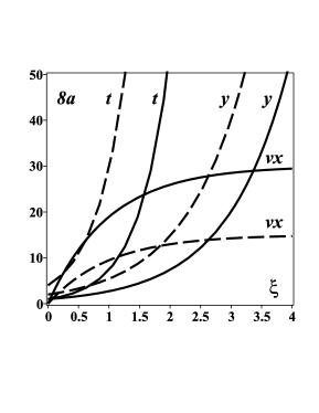
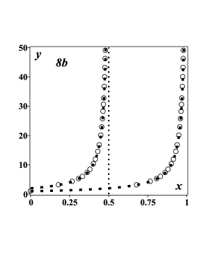
Figure 8: 8a — the dependences $x=x(\xi)$, $y=y(\xi)$, $t=t(\xi)$, obtained by numerical solution of the problem (94) for $b=1$, $\gamma=2$ with $a=1$ (solid lines) and $a=2$ (dashed lines) ($\nu=30$); 8b — numerical solutions of the problems (88) for $b=1$, $\gamma=2$ (circles) and (94) (points); for left curves $a=2$ and for right curves $a=1$.

The numerical solutions of the problems (88) and (94) for $b=1$, $\gamma=2$, obtained by the Runge–Kutta method of the fourth-order of approximation, are shown in Fig. 8 for $a=1$ and $a=2$. For a fixed step of integration, equal to $0.2$, the maximum difference between the exact solution (4) and the numerical solution of the related problem (94) is $0.0045\%$. For larger stepsizes, equal to $0.4$ and $0.6$, the maximum error in the numerical solutions is $0.061\%$ and $0.24\%$, respectively. It can be seen that the numerical solutions of the problems (88) and (94) are in a good agreement, but the rates of their approximation to the required asymptote $x=x_{*}$ are significantly different. For example, for the system (88), in order to obtain a good approximation to the asymptote, it is required to consider the interval $t\in[1,2400]$, and for the system (94) it suffices to take $\xi\in[0,4]$. Therefore, it should expect that the method based on the use of the system (93) with $g=t/y$ is much more efficient than the method based on the differential transformation.

For comparison, similar calculations were performed using Maple (2016), and applying the method based on the hodograph transformation (see Section 7.1, Item $1^{\circ}$) and the method of the arc-length transformation (see Section 7.1, Item $2^{\circ}$ for $c=1$ and $s=2$). In order to obtain a good approximation to the asymptote, applying the method based on the hodograph transformation, it is required to consider the interval $\xi\in[0,49]$, while using the method of the arc-length transformation leads to a significantly larger interval $\xi\in[0,2500]$. To control a numerical integration process, the calculations were carried out with the aid of two other most important and powerful mathematical software packages: Mathematica (11), and MATLAB (2016a). It was found that the method based on the use of the system (94) with $g=t/y$ is essentially more efficient than the method based on the hodograph transformation and the method of the arc-length transformation.

Example 20.

For the test problem (87), in which $f=b^{2}\gamma y^{2\gamma-1}$, we set $g=f/t$ (see Item $5^{\circ}$ in Section 7.1). Substituting these functions into (93), we arrive at the Cauchy problem

$$\begin{gathered}x^{\prime}_{\xi}=\frac{\mskip 1.0mut\mskip 1.0mu}{\mskip 1.0mub^{2}\gamma y^{2\gamma-1}\mskip 1.0mu},\quad\ y^{\prime}_{\xi}=\frac{\mskip 1.0mut^{2}\mskip 1.0mu}{\mskip 1.0mub^{2}\gamma y^{2\gamma-1}\mskip 1.0mu},\quad\ t^{\prime}_{\xi}=t\quad\ (\xi>0);\\ x(0)=0,\quad\ y(0)=a,\quad\ t(0)=a^{\gamma}b.\end{gathered}$$ (96)

The exact solution of this problem in parametric form is

$$x=\frac{\mskip 1.0mu1\mskip 1.0mu}{\mskip 1.0mua^{\gamma-1}b(\gamma-1)\mskip 1.0mu}\Bigl{[}1-e^{-(\gamma-1)\xi/\gamma}\Bigr{]},\quad\ y=ae^{\xi/\gamma},\quad\ t=a^{\gamma}be^{\xi}.$$ (97)

The required value $x=x(\xi)$ tends exponentially to the asymptotic value $\displaystyle x_{*}=\frac{\mskip 1.0mu1\mskip 1.0mu}{\mskip 1.0mua^{\gamma-1}b(\gamma-1)\mskip 1.0mu}$ as $\xi\to\infty$. However, in comparison with the method applied in Example 19, in this case the rate of approximation of the parametric solution to the asymptote is less (which is not important for application of the standard numerical methods for solving similar problems). Note that the solution (97) coincides with (95) if we redenote $\xi$ by $\gamma\xi$.

7.3 Generalizations based on the use of differential constraints

The method of numerical integration of the Cauchy problems with blow-up solutions, which based on introducing a non-local variable, can be generalized if the relation (92) is replaced by the first-order differential constraint

$$\xi^{\prime}_{x}=g(x,y,t,\xi)$$ (98)

with the initial condition $\xi(x=x_{0})=\xi_{0}$.

If we set $\xi_{0}=0$, then the use of the differential constraint (98) leads to the problem (93), where the function $g(x,y,t)$ must be replaced by $g(x,y,t,\xi)$ in the equations.

Using differential constraints increases the possibilities for numerical analysis of blow-up problems.

In particular, if we choose a differential constraint of the form (98) with

$$g(x,y,t,\xi)=\frac{\mskip 1.0mut\mskip 1.0mu}{\mskip 1.0mu\varphi(\xi)y+\psi(\xi)\mskip 1.0mu},$$ (99)

where $\varphi(\xi)$ and $\psi(\xi)$ are given functions, then the second equation of the system (93) is reduced to the linear equation for $y=y(\xi)$, the solution of which is well known. As a result, the considered system, consisting of three equations, is simplified and reduced to two equations.

If we choose a differential constraint of the form (98) with

$$g(x,y,t,\xi)=\frac{\mskip 1.0muf(x,y,t)\mskip 1.0mu}{\mskip 1.0mu\varphi(\xi)t+\psi(\xi)\mskip 1.0mu},$$ (100)

then the third equation of the system (93) is reduced to the linear equation for $t=t(\xi)$. In this case, the system under consideration also is reduced to two equations.

Example 21.

For the test Cauchy problem (87) with $b=1$ and $\gamma=2$, we take the differential constraint (98) with the function (100), where $f=2y^{3}$, $\varphi(\xi)=2(1+2\xi)$, and $\psi(\xi)=0$. As a result, we arrive at the following problem for the ODE system:

$$\begin{gathered}x^{\prime}_{\xi}=\frac{\mskip 1.0mut(1+2\xi)\mskip 1.0mu}{\mskip 1.0muy^{3}\mskip 1.0mu},\quad\ y^{\prime}_{\xi}=\frac{\mskip 1.0mut^{2}(1+2\xi)\mskip 1.0mu}{\mskip 1.0muy^{3}\mskip 1.0mu},\quad\ t^{\prime}_{\xi}=2t(1+2\xi)\quad\ (\xi>0);\\ x(0)=0,\quad\ y(0)=a,\quad\ t(0)=a^{2}.\end{gathered}$$ (101)

The exact solution of the problem in parametric form is

$$x=\frac{\mskip 1.0mu1\mskip 1.0mu}{\mskip 1.0mua\mskip 1.0mu}\bigl{(}1-e^{-\xi-\xi^{2}}\bigr{)},\quad\ y=ae^{\xi+\xi^{2}},\quad\ t=a^{2}e^{2(\xi+\xi^{2})}.$$ (102)

It can be seen that the required function $x=x(\xi)$ tends much faster to the asymptotic value $x_{*}=1/a$ as $\xi\to\infty$ than in Examples 19 and 20.

7.4 Comparison of efficiency of various transformations for numerical integration of second-order blow-up ODE problems

In Table 2, a comparison of the efficiency of the numerical integration methods, based on various non-local transformations of the form (92) and differential constraints of the form (98) is presented by using the example of the test blow-up problem for the second-order ODE (87) with $a=b=1$ and $\gamma=2$. The comparison is based on the number of grid points needed to make calculations with the same maximum error (approximately equal to $0.1$ and $0.005$).

Error${}_{{\rm max}},\%=0.1$
Transformation or	Function	Max. interval	Stepsize	Grid points
differential constraint	$g$	$\xi_{{\rm max}}\qquad$	$h\quad$	number $N$
Arc-length	$g{=}\sqrt{1{+}t^{2}{+}f^{2}}$	2500.0	0.4150	6024
Nonlocal, Item $2^{\circ}$	$g{=}1{+}|t|{+}|f|$	2544.0	0.7550	3369
Hodograph	$g{=}t$	49.2	0.4510	109
Special exp-type, Item $5^{\circ}$	$g{=}f/t$	7.807	0.2110	37
Diff. constraint, p.c. of (100)	$g{=}f/[2t(1+2\xi)]$	1.55	0.0470	33
Special exp-type, Item $4^{\circ}$	$g{=}t/y$	3.9	0.1300	30
Diff. constraint, p.c. of (99)	$g{=}t/[2(\xi+1)e^{2\xi+\xi^{2}}]$	1.218	0.0435	28
Error${}_{{\rm max}},\%=0.005$
Transformation or	Function	Max. interval	Stepsize	Grid points
differential constraint	$g$	$\xi_{{\rm max}}\qquad$	$h\quad$	number $N$
Arc-length	$g{=}\sqrt{1{+}t^{2}{+}f^{2}}$	2500.0	0.200	12500
Nonlocal, Item $2^{\circ}$	$g{=}1{+}|t|{+}|f|$	2544.0	0.350	7268
Hodograph	$g{=}t$	49.0	0.125	392
Special exp-type, Item $5^{\circ}$	$g{=}f/t$	7.821	0.099	79
Diff. constraint, p.c. of (100)	$g{=}f/[2t(1+2\xi)]$	1.55	0.021	74
Special exp-type, Item $4^{\circ}$	$g{=}t/y$	3.9	0.060	65
Diff. constraint, p.c. of (99)	$g{=}t/[2(\xi+1)e^{2\xi+\xi^{2}}]$	1.220	0.020	61

Table 2: Various types of analytical transformations applied for numerical integration of the problem (87) for $a=b=1$ and $\gamma=2$ with a given accuracy (percent errors are $0.1$ and $0.005$ for $\Lambda_{\text{m}}\leq 50$) and their basic parameters (maximum interval, stepsize, grid points number). The abbreviation “p.c.” stands for “particular case” and the notation $f=2y^{3}$ is used.

It can be seen that the arc-length transformation is the least effective, since the use of this transformation is associated with a large number of grid points. In particular, when using the last four transformations, you need 150–200 times less of a number of grid points. The hodograph transformation has an intermediate (moderate) efficiency. The use of the exp-type transformation with $g=t/y$ gives rather good results.

8 Second-order autonomous equations. Solution of the Cauchy problem. Simple estimates

We consider the Cauchy problem for the second-order autonomous equation of the general form

$$y^{\prime\prime}_{xx}=f(y)\quad(x>0),\quad\ y(0)=a,\quad\ y^{\prime}_{x}(0)=b.$$ (103)

We assume that $a>0$, $b\geq 0$ and $f(y)>0$ is a continuous function that is defined for all $y\geq a$.

It is not difficult to show that, the equation (103) admits a first integral. As a result, with allowance for the initial conditions, we arrive at the Cauchy problem for the first-order autonomous equation

$$\begin{gathered}y^{\prime}_{x}=F(y)\quad(x>0),\quad\ y(0)=a;\\ F(y)=\biggl{[}2\int^{y}_{a}f(z)\,dz+b^{2}\biggr{]}^{\!1/2},\end{gathered}$$ (104)

which coincides with the problem (49), up to obvious modifications in notations. Therefore, we can use the results of Section 5.1.

The exact solution of the Cauchy problem (104) is determined by the formula (50), in which the function $f(y)$ should be replaced by $F(y)$. In blow-up problems, the critical value $x_{*}$ is found by the formula (51), where the function $f(y)$ also must be replaced by $F(y)$.

Sufficient criterion of the existence of a blow-up solution. Suppose that for some $\kappa>0$ we have the limiting relation

$$\lim_{y\to\infty}\frac{\mskip 1.0muF(y)\mskip 1.0mu}{\mskip 1.0muy^{1+\kappa}\mskip 1.0mu}=s,\quad\ 0<s\leq\infty.$$ (105)

Then the solution of the Cauchy problem (103), when the above conditions are satisfied, is a blow-up solution.

The condition (105) is inconvenient, since it contains the function $F(y)$, which is rather complexly connected with the right-hand side $f(y)$ of the original equation (103). This condition can be simplified and transformed to a more convenient form:

$$\lim_{y\to\infty}\frac{\mskip 1.0muf(y)\mskip 1.0mu}{\mskip 1.0muy^{1+\kappa_{1}}\mskip 1.0mu}=s_{1},\quad\ 0<s_{1}\leq\infty,$$

where $\kappa_{1}$ is a positive number.

By applying the sufficient criterion, we obtain the following useful result.

The Cauchy problem (103) for an autonomous equation with power nonlinearity, $f(y)=cy^{\sigma}$ ($c>0$), has a blow-up solution if $\sigma>1$.

9 Blow-up problems for systems of ODEs

9.1 Method based on non-local transformations

We consider the Cauchy problem for a system consisting of $n$ first-order coupled ODEs of the general form

$$\frac{\mskip 1.0mudy_{m}\mskip 1.0mu}{\mskip 1.0mudx\mskip 1.0mu}=f_{m}(x,y_{1},\dots,y_{n}),\quad\ \ m=1,\dots,n\quad\ (x>x_{0}),$$ (106)

with the initial conditions

$$y_{m}(x_{0})=y_{m0},\quad\ \ m=1,\,2,\,\dots,\,n.$$ (107)

In blow-up problems, the right-hand side of at least one of the equations (106) (after substituting the solution into it) tends to infinity as $x\to x_{*}$, where the value $x_{*}$ is unknown in advance.

In the general case, the functions $f_{m}$ may have different signs. Further, we assume that $\displaystyle\sum^{n}_{m=1}|f_{m}|>0$.

We associate the system (106) with the equivalent system of equations consisting of $(n+1)$ equations

$$\hskip-12.0pt\frac{\mskip 1.0mudx\mskip 1.0mu}{\mskip 1.0mud\xi\mskip 1.0mu}=\frac{\mskip 1.0mu1\mskip 1.0mu}{\mskip 1.0mug(x,y_{1},\dots,y_{n})\mskip 1.0mu},\ \ \frac{\mskip 1.0mudy_{m}\mskip 1.0mu}{\mskip 1.0mud\xi\mskip 1.0mu}=\frac{\mskip 1.0muf_{m}(x,y_{1},\dots,y_{n})\mskip 1.0mu}{\mskip 1.0mug(x,y_{1},\dots,y_{n})\mskip 1.0mu},\ \ m{=}1,\dots,n\ \ (\xi{>}0)$$ (108)

with the initial conditions

$$x(0)=x_{0},\quad\ y_{m}(0)=y_{m0},\quad\ \ m=1,\,2,\,\dots,\,n.$$ (109)

Here $\xi$ is a non-local variable defined by the formula

$$\xi=\int^{x}_{x_{0}}g(x,y_{1},\dots,y_{n})\,dx,\quad\ y_{m}=y_{m}(x),\quad\ \ m=1,\dots,n\ \ \ (\xi\geq 0).$$ (110)

In (108), it is assumed that $g>0\,$ if $\displaystyle\,\sum^{n}_{m=1}|y_{m}|>0$. Below we will describe some possible ways of choosing the function $g=g(x,y_{1},\dots,y_{n})$.

9.2 Special cases of non-local transformations

Let us consider some possible ways of choosing the function $g$ in the system (108).

$1^{\circ}$. We can take

$$g=\Bigl{[}c_{0}+\sum^{n}_{m=1}c_{m}|f_{m}(x,y_{1},\dots,y_{n})|^{s}\Bigr{]}^{1/s},\ \ c_{0}>0,\ \ c_{m}>0,\ \ s>0.$$ (111)

In particular, if we set $c_{0}=c_{m}=s=1$ ($m=1,\dots,n$) in (111), then the system (108) takes the form

$$\frac{\mskip 1.0mudx\mskip 1.0mu}{\mskip 1.0mud\xi\mskip 1.0mu}=\frac{\mskip 1.0mu1\mskip 1.0mu}{\mskip 1.0mu\displaystyle 1{+}\sum^{n}_{m=1}|f_{m}(x,y_{1},\dots,y_{n})|\mskip 1.0mu},\ \ \frac{\mskip 1.0mudy_{m}\mskip 1.0mu}{\mskip 1.0mud\xi\mskip 1.0mu}=\frac{\mskip 1.0muf_{m}(x,y_{1},\dots,y_{n})\mskip 1.0mu}{\mskip 1.0mu\displaystyle 1{+}\sum^{n}_{m=1}|f_{m}(x,y_{1},\dots,y_{n})|\mskip 1.0mu},$$ (112)

where $m=1,\dots,n$.

Unlike the right-hand sides of the original system (106), the right-hand sides of the system (108) with (111) have no singularities since all the derivatives are bounded, $|(y_{m})^{\prime}_{\xi}|\leq 1$ ($m=1,\dots,n$); we recall that for blow-up solutions at least one of the derivatives $(y_{m})^{\prime}_{x}$ tends to infinity as $x\to x_{*}$.

The numerical solution of the problem (108)–(109) with (111) can be obtained, for example, applying the Runge–Kutta method or other standard numerical methods, see above.

$2^{\circ}$. For the system (108) with

$$g=\Bigl{[}1+\sum^{n}_{m=1}f^{2}_{m}(x,y_{1},\dots,y_{n})\Bigr{]}^{1/2},$$ (113)

we get the method of the arc-length transformation [4] (the function (113) is a particular case of (111) with $c_{0}=c_{m}=1$ and $s=2$). Therefore for blow-up problems, the method based on introducing the non-local variable (110) is more general than the method of the arc-length transformation.

$3^{\circ}$. In the general case, it is not known in advance whether the solution of the Cauchy problem (106)–(107) is a solution with usual properties, or is a blow-up solution. Therefore, in the first stage, the problem (106)–(107) can be solved by any standard fixed-step numerical method, for example, by the Runge–Kutta method. If one of the components, for example, $y_{k}$, begins to grow very rapidly (and increases faster than exponential and faster than the other components), then a hypothesis arises that the corresponding solution is a blow-up solution. Numerical confirmation of this hypothesis is a rapid growth of the ratio $|f_{k}/y_{k}|$ with increasing of the integration region with respect to $x$. In this case, it is reasonable to choose the function $g$ in (108), for example, as follows:

$$g=\frac{\mskip 1.0mu1\mskip 1.0mu}{\mskip 1.0muy_{k}\mskip 1.0mu}f_{k}(x,y_{1},\dots,y_{n}).$$ (114)

As a result, the $(k+1)$-th equation of the system (108) is easily integrated and, taking into account the corresponding initial condition (109), we arrive at the dependence

$$y_{k}=y_{k0}e^{\xi}.$$ (115)

Substituting the relations (114) and (115) into the remaining equations of the system (108), we obtain the Cauchy problem

$$\begin{gathered}\frac{\mskip 1.0mudx\mskip 1.0mu}{\mskip 1.0mud\xi\mskip 1.0mu}=\frac{\mskip 1.0muy_{k}\mskip 1.0mu}{\mskip 1.0muf_{k}(x,y_{1},\dots,y_{n})\mskip 1.0mu},\quad\ \frac{\mskip 1.0mudy_{m}\mskip 1.0mu}{\mskip 1.0mud\xi\mskip 1.0mu}=\frac{\mskip 1.0muy_{k}f_{m}(x,y_{1},\dots,y_{n})\mskip 1.0mu}{\mskip 1.0muf_{k}(x,y_{1},\dots,y_{n})\mskip 1.0mu},\\ m=1,\dots,n;\quad\ \text{$m\not=k$}\quad\ (\xi>0),\end{gathered}$$ (116)

with the initial conditions (109).

In the right-hand sides of the system (116), the function $y_{k}$ should be replaced by the right-hand side of the formula (115).

The numerical solution of the system (116) with (115) and the initial conditions (109) can be obtained, for example, by applying the Runge–Kutta method or the other standard numerical methods with a sufficiently large stepsize in $\xi$.

Example 22.

We consider the test Cauchy problem for the system of three equations

$$\begin{gathered}\frac{\mskip 1.0mudy_{1}\mskip 1.0mu}{\mskip 1.0mudx\mskip 1.0mu}=-y_{1}y_{2},\quad\ \frac{\mskip 1.0mudy_{2}\mskip 1.0mu}{\mskip 1.0mudx\mskip 1.0mu}=y_{2}^{4}y_{3},\quad\ \frac{\mskip 1.0mudy_{3}\mskip 1.0mu}{\mskip 1.0mudx\mskip 1.0mu}=-2y_{1};\\ y_{1}(0)=y_{2}(0)=y_{3}(0)=1.\end{gathered}$$ (117)

The exact solution of this problem has the form

$$y_{1}=1-x,\quad\ y_{2}=\frac{\mskip 1.0mu1\mskip 1.0mu}{\mskip 1.0mu1-x\mskip 1.0mu},\quad\ y_{3}=(1-x)^{2}.$$ (118)

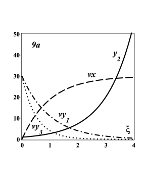
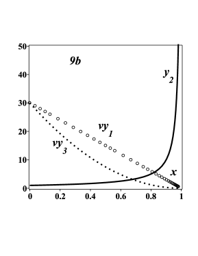
Figure 9: 9a — the dependences $x=x(\xi)$, $y_{1}=y_{1}(\xi)$, $y_{3}=y_{3}(\xi)$, obtained by numerical solution of the problem (119) ($\nu=30$), and $y_{2}=e^{\xi}$; 9b — numerical solution of the problem (119): $y_{1}(x)$ (circles), $y_{2}(x)$ (solid line), and $y_{3}(x)$ (points).

A trial numerical integration of the problem (117) by the Runge–Kutta method shows that the component $y_{2}$ grows faster (in magnitude) that the other components. Using the formulas (114) and (115), we obtain that $g=y_{2}^{3}y_{3}$ and $y_{2}=e^{\xi}$. Substituting these functions into (116), and taking into account that $f_{1}=-y_{1}y_{2}$ and $f_{3}=-2y_{1}$, we arrive at the equivalent Cauchy problem

$$\begin{gathered}\frac{\mskip 1.0mudx\mskip 1.0mu}{\mskip 1.0mud\xi\mskip 1.0mu}=\frac{\mskip 1.0mue^{-3\xi}\mskip 1.0mu}{\mskip 1.0muy_{3}\mskip 1.0mu},\quad\ \frac{\mskip 1.0mudy_{1}\mskip 1.0mu}{\mskip 1.0mud\xi\mskip 1.0mu}=-\frac{\mskip 1.0mue^{-2\xi}y_{1}\mskip 1.0mu}{\mskip 1.0muy_{3}\mskip 1.0mu},\quad\ \frac{\mskip 1.0mudy_{3}\mskip 1.0mu}{\mskip 1.0mud\xi\mskip 1.0mu}=-\frac{\mskip 1.0mu2e^{-3\xi}y_{1}\mskip 1.0mu}{\mskip 1.0muy_{3}\mskip 1.0mu};\\ x(0)=0,\quad\ y_{1}(0)=y_{3}(0)=1.\end{gathered}$$ (119)

Unlike the original problem (117), the problem (119) does not have blow-up singularities. Its exact solution is written in parametric form as follows:

$$x=1-e^{-\xi},\quad y_{1}=e^{-\xi},\quad\ y_{2}=e^{\xi},\quad\ y_{3}=e^{-2\xi}.$$ (120)

The numerical solution of the problem (119) is shown in Fig. 9. We do not present here the exact dependences (120), since they almost coincide (up to the maximum error $0.025\%$) with the results of the numerical solution.

Remark 14.

In the methods described in Items $1^{\circ}$ and $2^{\circ}$, the rate of approximation of the function $x=x(\xi)$ to the asymptote, that determines the singular point $x_{*}$, will be power-law behavior with respect to $\xi$, while the method presented in Item $3^{\circ}$, yields the exponential rate of approximation of the singular point.

Remark 15.

For systems of equations (106) of polynomial type, the most growing component $y_{k}$ can be determined by substituting the approximate functions $y_{1}=\alpha_{1}(x_{*}-x)^{-\beta_{1}}$, …, $y_{n}=\alpha_{n}(x_{*}-x)^{-\beta_{n}}$ into the equations. Then, from the analysis of the obtained algebraic relations, the largest exponent $\beta_{k}=\max[\beta_{1},\dots,\beta_{n}]$ is found, where $\beta_{k}>0$. The component $y_{k}$ is used in formula (114) for the function $g$.

Example 23.

Consider the problem (117). The solution in the neighborhood of the singular point is sought in the form

$$y_{1}=\alpha_{1}(x_{*}-x)^{-\beta_{1}},\quad\ y_{2}=\alpha_{2}(x_{*}-x)^{-\beta_{2}},\quad\ y_{3}=\alpha_{3}(x_{*}-x)^{-\beta_{3}}.$$ (121)

Substituting the expressions (121) into (117), we obtain a simple system of linear algebraic equations for the exponents $\beta_{m}$ ($m=1,\,2,\,3$). The solution of the system is

$$\beta_{1}=-1,\quad\ \beta_{2}=1,\quad\ \beta_{3}=-2.$$

The maximum exponent is $\beta_{2}$. Therefore, the component $y_{2}$ should be used for the function $g$ in formula (114).

Remark 16.

If the two components, $y_{k}$ and $y_{j}$, simultaneously have a blow-up behavior (with the same or different rate of approaching to infinity as $x\to x_{*}$), then we also can choose, for example, $g=c+|f_{k}|+|f_{j}|$ or $g=c_{1}+\sqrt{c_{2}+f_{k}^{2}+f_{j}^{2}}$ in (108). Here $c$, $c_{1}$, and $c_{2}$ are some non-negative constants.

Remark 17.

The technique developed in Section 9 can also be used in Cauchy problems for partial differential equations (PDEs) with blow-up solutions, if to apply the methods leading to systems of ODEs (for example, in projection methods and the method of lines [37, 38]).

9.3 Method based on differential constraints

For the Cauchy problems that are described by the systems of ODEs and have blow-up solutions, the method of numerical integration, based on introducing a non-local variable, can be generalized if, instead of the relation (110) to take the first-order differential constraint

$$\xi^{\prime}_{x}=g(x,y_{1},\dots,y_{n},\xi)$$ (122)

with the initial condition $\xi(x=x_{0})=\xi_{0}$.

If we set $\xi_{0}=0$, then the use of the differential constraint (122) leads to the problem (108), where the function $g(x,y_{1},\dots,y_{n})$ must be replaced by the function $g(x,y_{1},\dots,y_{n},\xi)$ in the equations.

10 Blow-up problems for higher-order ODEs

10.1 Reduction of higher-order ODEs to a system of first-order ODEs

Consider the Cauchy problem for the $n$ th-order ODE:

$$\begin{gathered}y^{(n)}_{x}=f(x,y,y^{\prime}_{x},\dots,y^{(n-1)}_{x})\quad\ (x>x_{0});\\ y(x_{0})=y_{0},\quad y^{\prime}_{x}(x_{0})=y^{(1)}_{0},\quad\ldots,\quad y^{(n-1)}_{x}(x_{0})=y^{(n-1)}_{0},\end{gathered}$$ (123)

where $y^{(k)}_{x}=d^{k}y/dx^{k}$ ($k=3,\dots,n$).

The Cauchy problem for one $n$ th-order ODE (123) is equivalent to the Cauchy problem for a system of $n$ coupled first-order equations of the special form

$$\begin{gathered}y^{\prime}_{1}=y_{2},\quad\ y^{\prime}_{2}=y_{3},\quad\ \dots,\quad\ y^{\prime}_{n-1}=y_{n},\quad\ y_{n}^{\prime}=f(x,y_{1},y_{2},\ldots,y_{n});\\ y_{1}(x_{0})=y_{0},\quad y_{2}(x_{0})=y^{(1)}_{0},\quad\ldots,\quad y_{n}(x_{0})=y^{(n-1)}_{0},\end{gathered}$$ (124)

where the prime denotes the derivative with respect to $x$ and $y_{1}\equiv y$.

The problem (124) is a particular case of the Cauchy problem (106)–(107) and the general methods described in Sections 9.1 and 9.2 are applicable to it.

10.2 Blow-up problems for third-order ODEs

Let us consider the Cauchy problem for the nonlinear third-order ODE of the general form

$$y^{\prime\prime\prime}_{xxx}=f(x,y,y^{\prime},y^{\prime\prime}_{xx})\quad(x>0);\quad y(0)=y_{0},\ y^{\prime}_{x}(0)=y_{1},\ y^{\prime\prime}_{xx}(0)=y_{2}.$$ (125)

The problem for one third-order ODE (125) is equivalent to the following problem for the system of three coupled first-order equations:

$$\begin{gathered}y^{\prime}_{x}=t,\quad\ t^{\prime}_{x}=w,\quad\ w^{\prime}_{x}=f(x,y,t,w)\quad\ \ (x>0);\\ y(0)=y_{0},\quad\ t(0)=y_{1},\quad\ w(0)=y_{2}.\end{gathered}$$ (126)

The introduction of the non-local variable (110) transforms the system (126) to the form

$$\begin{gathered}x^{\prime}_{\xi}=\frac{\mskip 1.0mu1\mskip 1.0mu}{\mskip 1.0mug\mskip 1.0mu},\quad\ y^{\prime}_{\xi}=\frac{\mskip 1.0mut\mskip 1.0mu}{\mskip 1.0mug\mskip 1.0mu},\quad\ t^{\prime}_{\xi}=\frac{\mskip 1.0muw\mskip 1.0mu}{\mskip 1.0mug\mskip 1.0mu},\quad\ w^{\prime}_{\xi}=\frac{\mskip 1.0muf\mskip 1.0mu}{\mskip 1.0mug\mskip 1.0mu}\quad\ \ (\xi>0);\\ x(0)=0,\quad\ y(0)=y_{0},\quad\ t(0)=y_{1},\quad\ w(0)=y_{2},\end{gathered}$$ (127)

where $f=f(x,y,t,w)$ and $g=g(x,y,t,w)$.

Let us consider various possibilities for choosing the function $g$ in the system (127).

$1^{\circ}$. We can take $g=\bigl{(}c_{1}+c_{2}|t|^{s}+c_{3}|w|^{s}+c_{4}|f|^{s}\bigr{)}^{1/s}$ for $c_{m}>0$ and $s>0$. The case $c_{1}=c_{2}=c_{3}=c_{4}=1$ and $s=2$ corresponds to the method of the arc-length transformation [4].

$2^{\circ}$. We can take $g=t/y$ (or $g=kt/y$, where $k>0$ is a constant). In this case, the system (127) is simplified, since the second equation is directly integrated, and taking into account the second initial condition, we obtain $y=y_{0}e^{\xi}$.

$3^{\circ}$. We can take $g=w/t$ (or $g=kw/t$ with $k>0$). In this case, the system (127) is simplified, since the third equation is directly integrated, and we obtain $t=y_{1}e^{\xi}$. Taking into account the relations (126), we also have

$$\xi=\int^{x}_{x_{0}}\frac{\mskip 1.0muw\mskip 1.0mu}{\mskip 1.0mut\mskip 1.0mu}\,dx=\int^{x}_{x_{0}}\frac{\mskip 1.0muy^{\prime\prime}_{xx}\mskip 1.0mu}{\mskip 1.0muy^{\prime}_{x}\mskip 1.0mu}\,dx=\ln\frac{\mskip 1.0muy^{\prime}_{x}\mskip 1.0mu}{\mskip 1.0muy_{1}\mskip 1.0mu}.$$

Thus, this non-local transformation coincides with the modified differential transformation, which was considered in Section 2.3.

$4^{\circ}$. Also, we can take $g=f/w$ (or $g=kf/w$ with $k>0$). In this case, the system (127) is also simplified, since the fourth equation is directly integrated, and we obtain $w=y_{2}e^{\xi}$.

The transformations corresponding to the last three cases, $2^{\circ}$, $3^{\circ}$, and $4^{\circ}$, will be called the special exp-type transformations, they lead to the solutions, in which the variable $x$ tends exponentially rapidly to a blow-up point $x_{*}$.

Example 24.

We consider in more detail the test Cauchy problem of the form

$$y^{\prime\prime\prime}_{xxx}=6y^{4}\quad\ \ (x>0);\quad y(0)=y^{\prime}_{x}(0)=1,\quad y^{\prime\prime}_{xx}(0)=2.$$ (128)

The exact solution of this problem is determined by the formula (4).

In Table 3, a comparison of the efficiency of the numerical integration methods, based on various non-local transformations of the form (92) is presented by using the example of the test blow-up problem for the third-order ODE (128). The comparison is based on the number of grid points needed to make calculations with the same maximum error (e.g., equal to $0.1$ and $0.01$).

Error${}_{{\rm max}},\%=0.1$
Transformation	Function $g$	Max. interval	Stepsize	Grid points
		$\xi_{{\rm max}}\qquad$	$h\quad$	number $N$
Arc-length, Item $1^{\circ}$	$g{=}\sqrt{1{+}t^{2}{+}w^{2}{+}f^{2}}$	249600.000	0.7800	320000
Nonlocal, Item $1^{\circ}$	$g{=}1{+}|t|{+}|w|+|f|$	252000.000	1.4000	180000
Hodograph	$g{=}t$	49.010	0.1690	290
Special exp-type, Item $4^{\circ}$	$g{=}f/w$	11.741	0.2498	47
Special exp-type, Item $2^{\circ}$	$g{=}t/y$	3.912	0.0978	40
Special exp-type, Item $3^{\circ}$	$g{=}w/t$	7.828	0.2060	38
Error${}_{{\rm max}},\%=0.01$
Transformation	Function $g$	Max. interval	Stepsize	Grid points
		$\xi_{{\rm max}}\qquad$	$h\quad$	number $N$
Arc-length, Item $1^{\circ}$	$g{=}\sqrt{1{+}t^{2}{+}w^{2}{+}f^{2}}$	252000.000	0.4500	560000
Nonlocal, Item $1^{\circ}$	$g{=}1{+}|t|{+}|w|+|f|$	253580.000	0.8180	310000
Hodograph	$g{=}t$	49.020	0.0950	516
Special exp-type, Item $4^{\circ}$	$g{=}f/w$	11.738	0.1381	85
Special exp-type, Item $2^{\circ}$	$g{=}t/y$	3.920	0.0560	70
Special exp-type, Item $3^{\circ}$	$g{=}w/t$	7.827	0.1223	64

Table 3: Various types of analytical transformations applied for numerical integration of the problem (128) with a given accuracy (percent errors are $0.1$ and $0.01$ for $\Lambda_{\text{m}}\leq 50$) and their basic parameters (maximum interval, stepsize, grid points number).

It can be seen that the arc-length transformation is the least effective, since the use of this transformation is associated with a large number of grid points. In particular, when using the last three transformations, you need 6580–8750 times less of a number of grid points. The hodograph transformation has an intermediate (moderate) efficiency. The use of the last three special exp-type transformations with $g=f/w$, $g=t/y$, and $g=w/t$ gives rather good results. Note that an even smaller number of grid points can be obtained by using suitable differential constraints.

11 Elementary approaches allowing one to find the form of new variables

We now describe an elementary approach, based on simple semi-geometric considerations, which allows us to find the form of new variables that transform the original blow-up problem to a problem, more suitable for numerical integration, that does not have blow-up singularities.

11.1 Combination of point transformation and hodograph transformation

Let us consider the approximate relation (1) as an equation connecting the variables $x$ and $y$. Solving it with respect to $x$ (for concreteness, we assume that $A>0$), we obtain

$$x=x_{*}-B_{1}y^{-1/\beta},\quad\ \ B_{1}=A^{1/\beta}.$$ (129)

It is seen that $x$ tends to the blow-up point $x_{*}$ slowly enough as $y\to\infty$ (by the power law $\sim y^{-1/\beta}$). If we make the substitution $y=e^{\xi}$, then the rate of approximation to the desired asymptotic value $x_{*}$ will become exponential with respect to the new variable $\xi$ (i.e., will increase significantly). It is convenient to represent the described procedure in the form of a transformation

$$\xi=\ln y,\quad\ z=x,$$ (130)

where $z=z(\xi)$ is the new unknown function. As a result, we arrive at the dependence $z=x_{*}-B_{1}e^{-\xi/\beta}$, which can be written in the parametric form

$$x=x_{*}-B_{1}e^{-\xi/\beta},\quad\ y=e^{\xi}.$$ (131)

The transformation (130) is a combination of two simple point transformations: 1) the non-linear transformation $\bar{x}=x$, $\bar{y}=\ln y$ and 2) the hodograph transformation $\xi=\bar{y}$, $z=\bar{x}$. The transformation (130) is equivalent to the transformation (24) if $g=f/y$ (see Section 3.1, Item $5^{\circ}$) and to the transformation (92) if $g=t/y$ (see Section 7.1, Item $5^{\circ}$).

11.2 Combination of transformation, based on a differential variable, and point transformation

Differentiating the asymptotics (1), we have the following relations:

$$y^{\prime}_{x}=A\beta(x-x_{*})^{-\beta-1},\quad\ y=A\biggl{(}\frac{\mskip 1.0muy^{\prime}_{x}\mskip 1.0mu}{\mskip 1.0muA\beta\mskip 1.0mu}\biggr{)}^{\textstyle\!\frac{\mskip 1.0mu\beta\mskip 1.0mu}{\mskip 1.0mu\beta+1\mskip 1.0mu}}$$ (132)

(the second relation is obtained from the first one after elimination of $x$ by means of (1)).

Excluding $y$ from (129) with the help of the second relation (132), we obtain

$$x=x_{*}-B_{2}(y^{\prime}_{x})^{\textstyle-\frac{\mskip 1.0mu1\mskip 1.0mu}{\mskip 1.0mu\beta+1\mskip 1.0mu}},\quad\ B_{2}=(A\beta)^{\textstyle\frac{\mskip 1.0mu1\mskip 1.0mu}{\mskip 1.0mu\beta+1\mskip 1.0mu}}.$$ (133)

It is seen that $x$ tends to the blow-up point $x_{*}$ slowly enough as $y^{\prime}_{x}\to\infty$ (in accordance with the power law $\sim(y^{\prime}_{x})^{-1/(\beta+1)}$).

If we make the substitution $y^{\prime}_{x}=e^{\xi}$, then the rate of approximation to the desired asymptotic value $x_{*}$ will become exponential with respect to the new variable $\xi$ (i.e., will increase significantly). The described procedure can be represented as a transformation

$$\xi=\ln y^{\prime}_{x},\quad\ x=x(\xi),\quad\ y=y(\xi),$$ (134)

which is based on a combination of the differential transformation $t=y^{\prime}_{x}$ (see Sections 2.1 and 6.1) and the point transformation $\xi=\ln t$.

The transformation (134) determines the asymptotics of the solution (1) in a neighborhood of the blow-up singularity in the parametric form

$$x=x_{*}-B_{2}e^{-\frac{\mskip 1.0mu1\mskip 1.0mu}{\mskip 1.0mu\beta+1\mskip 1.0mu}\xi},\quad\ y=AB_{2}^{-\beta}e^{\frac{\mskip 1.0mu\beta\mskip 1.0mu}{\mskip 1.0mu\beta+1\mskip 1.0mu}\xi}.$$ (135)

In Section 2.3, apart from other considerations, it was described how one can obtain a transformation of the type (134).

11.3 Relation allowing one to control the calculation process

We now derive a useful formula that makes it possible to control the calculation process.

Taking into account the relations (1) and (132), we differentiate the relation $y/y^{\prime}_{x}$. After elementary transformations, we obtain

$$\frac{\mskip 1.0mu1\mskip 1.0mu}{\mskip 1.0mu\beta\mskip 1.0mu}=\frac{\mskip 1.0muyy^{\prime\prime}_{xx}\mskip 1.0mu}{\mskip 1.0mu(y^{\prime}_{x})^{2}\mskip 1.0mu}-1=\frac{\mskip 1.0muy\mskip 1.0mu}{\mskip 1.0muy^{\prime}_{\xi}\mskip 1.0mu}\biggl{(}\frac{\mskip 1.0muy^{\prime\prime}_{\xi\xi}\mskip 1.0mu}{\mskip 1.0muy^{\prime}_{\xi}\mskip 1.0mu}-\frac{\mskip 1.0mux^{\prime\prime}_{\xi\xi}\mskip 1.0mu}{\mskip 1.0mux^{\prime}_{\xi}\mskip 1.0mu}\biggr{)}-1,$$ (136)

where $x=x(\xi)$, $y=y(\xi)$ is the representation of the solution in the parametric form.

For blow-up problems with a power singularity, the constant $\beta$ must be greater than zero. Therefore, for numerical representation of solutions in the parametric form, for large values of $\xi$ the right-hand side of (136) must tend to a positive constant (asymptote), which allows us to control the calculation process.

12 Brief conclusions

Three new methods of numerical integration of Cauchy problems for nonlinear ODEs of the first and second-order, which have a blow-up solution, are described. These methods are based on differential and non-local transformations, and also on differential constraints, that lead to the equivalent problems for systems of equations, whose solutions are represented in parametric form and have no singularities.

It is shown that:

(i) the method based on a non-local transformation of the general form includes themselves, as particular cases, the method based on the hodograph transformation, the method of the arc-length transformation, and the methods based on the differential and modified differential transformations;

(ii) the methods based on the exp-type and modified differential transformations are much more efficient than the method based on the hodograph transformation, the method of the arc-length transformation, and the method based on the differential transformation;

(iii) the method based on the differential constraints is the most general of the proposed methods.

In the Cauchy problems described by the first-order equations, two-sided theoretical estimates are established for the critical value of the independent variable $x=x_{*}$, when an unlimited growth of the solution occurs as approaching it.

It is shown that the method based on a non-local transformation of the general form as well as the method based on the differential constraints admit generalizations to the $n$ th-order ordinary differential equations and systems of coupled differential equations.

Note. In the near future, the authors are going to submit an article on the topic “Numerical integration of non-monotonic blow-up problems based on non-local transformations”.

References

- [1] M. Stuart, M. S. Floater. On the computation of blow-up, European J. Applied Math., 1990, vol. 1, No. 1, pp. 47–71.
- [2] E. A. Alshina, N. N. Kalitkin, P.V. Koryakin. Diagnostics of singularities of exact solutions in computations with error control (in Russian), Zh. Vychisl. Mat. Mat. Fiz., 2005, vol. 45, No. 10, pp. 1837–1847; http://eqworld.ipmnet.ru/ru/solutions/interesting/alshina2005.pdf
- [3] G. Acosta, G. Durán, J. D. Rossi. An adaptive time step procedure for a parabolic problem with blow-up. Computing, 2002, vol. 68, pp. 343–373.
- [4] S. Moriguti, C. Okuno, R. Suekane, M. Iri, K. Takeuchi. Ikiteiru Suugaku – Suuri Kougaku no Hatten (in Japanese). Baifukan, Tokyo, 1979.
- [5] C. Hirota, K. Ozawa. Numerical method of estimating the blow-up time and rate of the solution of ordinary differential equations – An application to the blow-up problems of partial differential equations, J. Comput. & Applied Math., 2006, vol. 193, No. 2, pp. 614–637.
- [6] R. Meyer-Spasche, Difference schemes of optimum degree of implicitness for a family of simple ODEs with blow-up solutions, J. Comput. and Appl. Mathematics, 1998, Vol. 97, pp. 137–152.
- [7] A. Goriely and C. Hyde, Finite time blow-up in dynamical systems, Phys. Letters A, 1999, Vol. 250, pp. 4–6.
- [8] U. Elias and H. Gingold, Critical points at infinity and blow-up of solutions of autonomous polynomial differential systems via compactification, J. Math. Anal. Appl., 2006, Vol. 318, pp. 305–322.
- [9] J. Baris, P. Baris, and B. Ruchlewicz, Blow-up solutions of quadratic differential systems, J. Math. Sciences, 2008, Vol. 149, No. 4, pp 1369–1375.
- [10] N. R. Nassif, N. Makhoul-Karamb, and Y. Soukiassian, Computation of blowing-up solutions for second-order differential equations using re-scaling techniques, J. Comput. Applied Math., 2009, Vol. 227, 185–195.
- [11] P. G. Dlamini, M. Khumalo. On the computation of blow-up solutions for semilinear ODEs and parabolic PDEs, Math. Problems in Eng., 2012, vol. 2012, Article ID 162034, 15 p.
- [12] Y.C. Zhou, Z. W. Yang, H. Y. Zhang, and Y. Wang, Theoretical analysis for blow-up behaviors of differential equations with piecewise constant arguments, Appl. Math. Comput., 2016, Vol. 274, pp. 353–361.
- [13] A. Takayasu, K. Matsue, T. Sasaki, K. Tanaka, M. Mizuguchi, S. Oishi. Numerical validation of blow-up solutions of ordinary differential equations. J. Comput. Applied Mathematics, 2017, vol. 314, pp. 10–29.
- [14] J. C. Butcher. The Numerical Analysis of Ordinary Differential Equations: Runge–Kutta and General Linear Methods. Wiley-Interscience, New York, 1987.
- [15] L. Fox and D. F. Mayers, Numerical Solution of Ordinary Differential Equations for Scientists and Engineers, Chapman & Hall, 1987.
- [16] J. D. Lambert, Numerical Methods for Ordinary Differential Systems, Wiley, New York, 1991.
- [17] W. E. Schiesser. Computational Mathematics in Engineering and Applied Science: ODEs, DAEs, and PDEs. CRC Press, Boca Raton, 1994.
- [18] L. F. Shampine, Numerical Solution of Ordinary Differential Equations, Chapman & Hall/CRC Press, Boca Raton, 1994.
- [19] U. M. Ascher, L. R. Petzold. Computer Methods for Ordinary Differential Equations and Differential-Algebraic Equations. SIAM, Philadelphia, 1998.
- [20] G. A. Korn, T. M. Korn. Mathematical Handbook for Scientists and Engineers, 2nd Edition. New York: Dover Publ., 2000.
- [21] I. K. Shingareva, C. Lizárraga-Celaya. Maple and Mathematica. A Problem Solving Approach for Mathematics, 2nd Edition. Springer, Wien – New York, 2009.
- [22] D. Griffiths, D. J. Higham. Numerical Methods for Ordinary Differential Equations. Springer, Wien – New York, 2010.
- [23] V. F. Zaitsev, A. D. Polyanin. Handbook of Nonlinear Differential Equations: Applications in Mechanics, Exact Solutions (in Russian), Nauka, Moscow, 1993.
- [24] V. F. Zaitsev, A. D. Polyanin. Discrete-Group Methods for Integrating Equations of Nonlinear Mechanics. CRC Press – Begell House, Boca Raton, 1994.
- [25] C. Muriel and J. L. Romero. Nonlocal transformations and linearization of second-order ordinary differential equations, J. Physics A: Math. Theor., Vol. 43, No. 43, 434025.
- [26] N. A. Kudryashov and D. I. Sinelshchikov. On the integrability conditions for a family of Liénard-type equations, Regular and Chaotic Dynamics, 2016, Vol. 21, No. 5, pp. 548–555.
- [27] N. A. Kudryashov and D. I. Sinelshchikov. On the criteria for integrability of the Liénard equation, Applied Mathematics Letters, 2016, Vol. 57, pp. 114–120.
- [28] A.D. Polyanin, V.F. Zaitsev, Handbook of Nonlinear Partial Differential Equations, 2nd Edition, Chapman & Hall/CRC Press, Boca Raton–London, 2012.
- [29] S. G. Mikhlin, Kh. L. Smolitsky. Approximate methods for solving differential and integral equations. (in Russian), Nauka, Moscow, 1965.
- [30] E. Kamke. Differentialgleichungen: Lösungsmethoden und Lösungen, I, Gewöhnliche Differentialgleichungen. B.G. Teubner, Leipzig, 1977.
- [31] A. D. Polyanin, V. F. Zaitsev. Handbook of Exact Solutions for Ordinary Differential Equations, 2nd Edition. Chapman & Hall/CRC Press, Boca Raton – London, 2003.
- [32] G. M. Murphy. Ordinary Differential Equations and Their Solutions. D. Van Nostrand, New York, 1960.
- [33] N. A. Kudryashov. Analytical Theory of Nonlinear Differential Equations (in Russian). Institute of Computer Science, Moscow – Izhevsk, 2004.
- [34] A. D. Polyanin and A. I. Zhurov. Parametrically defined nonlinear differential equations and their solutions: Applications in fluid dynamics. Applied Mathematics Letters, 2016, vol. 55, pp. 72–80.
- [35] A. D. Polyanin and A. I. Zhurov. Parametrically defined nonlinear differential equations, differential algebraic equations, and implicit ODEs: Transformations, general solutions, and integration methods, Applied Mathematics Letters, 2017, vol. 64, pp. 59–66.
- [36] A. D. Polyanin and I. K. Shingareva. The use of differential and non-local transformations for numerical integration of non-linear blow-up problems, Int. J. Non-Linear Mechanics, 2017, Vol. 95, pp. 178–184.
- [37] W. E. Schiesser, The Numerical Method of Lines, Academic Press, 1991 [see, also, S. Hamdi, W. E. Schiesser, and G. W. Griffiths, Method of lines, Scholarpedia, 2007, 2(7):2859; doi:10.4249/scholarpedia.2859].
- [38] W. E. Schiesser and G. W. Griffiths, A Compendium of Partial Differential Equation Models: Method of Lines Analysis with Matlab, Cambridge University Press, 2009.