Vibrationally resolved electronic spectra including vibrational pre-excitation: Theory and application to VIPER spectroscopy

Abstract

Vibrationally resolved electronic absorption spectra including the effect of vibrational pre-excitation are computed in order to interpret and predict vibronic transitions that are probed in the Vibrationally Promoted Electronic Resonance (VIPER) experiment [L. J. G. W. van Wilderen et al., Angew. Chem. Int. Ed. 53, 2667 (2014)]. To this end, we employ time-independent and time-dependent methods based on the evaluation of Franck-Condon overlap integrals and Fourier transformation of time-domain wavepacket autocorrelation functions, respectively. The time-independent approach uses a generalized version of the FCclasses method [F. Santoro et al., J. Chem. Phys. 126, 084509 (2007)]. In the time-dependent approach, autocorrelation functions are obtained by wavepacket propagation and by evaluation of analytic expressions, within the harmonic approximation including Duschinsky rotation effects. For several medium-sized polyatomic systems, it is shown that selective pre-excitation of particular vibrational modes leads to a redshift of the low-frequency edge of the electronic absorption spectrum, which is a prerequisite for the VIPER experiment. This effect is typically most pronounced upon excitation of modes that are significantly displaced during the electronic transition, like ring distortion modes within an aromatic $\pi$-system. Theoretical predictions as to which modes show the strongest VIPER effect are found to be in excellent agreement with experiment.

I Introduction

Combined electronic-vibrational spectroscopies pave the way for new strategies of probing and controlling molecular systems.van Wilderen and Bredenbeck (2015) This is exemplified by the recently introduced Vibrationally Promoted Electronic Resonance (VIPER) experiment van Wilderen and Bredenbeck (2015); van Wilderen, Messmer, and Bredenbeck (2014) where selective infrared (IR) excitation in the electronic ground state precedes visible (VIS) excitation, as sketched in Fig. 1. The VIPER pulse sequence was originally designed in the context of chemical exchangevan Wilderen, Messmer, and Bredenbeck (2014), but also lends itself to inducing selective cleavage of photolabile protecting groups through the use of selective IR excitation and isotope substitution. For example, substitution of ¹²C by ¹³C leaves the electronic absorption spectrum of bright transitions virtually unchanged while the frequencies of vibrational modes can be altered significantly. Different isotopomers can therefore be distinguished by their IR spectra and selectively excited using narrow-band IR pulses Kern-Michler et al. .

In the present work, we compute vibrationally resolved electronic absorption spectra including the effect of vibrational pre-excitation, in order to predict VIPER-active modes for several polyatomic chromophores, some of which have already been experimentally investigated. Notably, the laser dye Coumarin 6 is studied, which has served for demonstration of VIPER’s capability to measure exchange beyond the vibrational $T_{1}$ lifetimevan Wilderen and Bredenbeck (2015). Furthermore, [7-(diethylamino)coumarin-4-yl]methyl-azide (DEACM-N₃) and para-Hydroxyphenacyl thiocyanate (pHP-SCN) are investigated, which are model systems for photo-cleavable caging groupsKlán et al. (2012); Park and Givens (1997); van Wilderen et al. (2017), with the azide and thiocyanate groups representing the relevant leaving groups. We aim to establish a general understanding of which properties favor large spectral shifts that permit effective VIPER excitation. While we do not simulate the complete VIPER pump-probe sequencevan Wilderen and Bredenbeck (2015); van Wilderen, Messmer, and Bredenbeck (2014), our analysis of the vibronic spectra resulting from the combined IR-pump/VIS-pump steps, is suitable for the prediction of the relevant VIPER shifts.

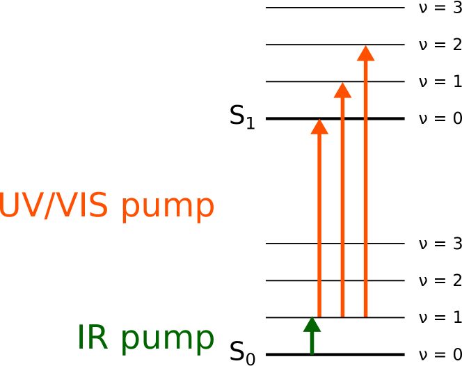
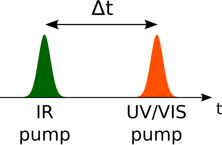
Figure 1: Left: The mixed IR/VIS VIPER excitation scheme. Right: Time-domain VIPER excitation sequence.

Figure 2: Structure of Coumarin 6 (A), DEACM-N₃, i.e., [7-(diethylamino)coumarin-4-yl]methyl-azide (B) and $p$HP-SCN, i.e., para-hydroxyphenacyl thiocyanate (C).

We apply both time-independent (TI) and time-dependent (TD) methods in conjunction with a quadratic vibronic model Hamiltonian that is parametrized in the full normal-mode space, based upon ground-state and excited-state electronic structure calculations. Besides displacements of the equilibrium geometry, the Hamiltonian accurately represents Duschinsky rotation effects.

The TI approach uses a generalized version of the FCclasses method developed by one of usSantoro et al. (2007a, b, 2008), where a pre-screening technique is adopted to select the relevant Franck-Condon (FC) overlap integrals and obtain fully converged spectra even for high-dimensional molecular systems. In the present context, this approach was specifically adapted such as to include selective vibrational pre-excitation.

In a complementary fashion, TD methods are employed in order to compute wavepacket autocorrelation functions, whose Fourier transforms yield the vibronic absorption spectrum. Within the harmonic approximation and including vibrational pre-excitation, autocorrelation functions are either computed analytically or else using the Multi-Layer Multiconfiguration Time-Dependent Hartree (ML-MCTDH) methodWang and Thoss (2003); Vendrell and Meyer (2011), a recently developed variant of the MCTDH method Meyer, Manthe, and Cederbaum (1990); Beck et al. (2000); Worth et al. (2008). In the present context, all methods are expected to give the same results for zero-temperature calculations including pre-excitation, but the efficiency of these methods differs as a function of dimensionality and type of vibrational pre-excitation.

The remainder of the manuscript is organized as follows. Sec. II details the TI and TD approaches employed in this study and Sec. III introduces an analysis in terms of spectral moments. Sec. IV summarizes the computational procedure, and Sec. V presents results obtained for three representative chromophores, together with experimental results for two of these systems. Sec. VI gives a discussion of the results and Sec. VII concludes. Finally, several Appendixes add information complementary to the main text.

II Methods for the computation of vibrationally resolved electronic spectra from a vibrationally pre-excited state

Conventionally, the computation of vibrationally resolved electronic spectra proceeds from a thermally averaged ensemble of excited vibrational states, populated according to a Boltzmann distributionSantoro et al. (2007b). In contrast, the present study is concerned with vibronic excitation from a non-equilibrium state where a single vibrational normal mode is placed into its first excited state by vibrational pre-excitation, while all other normal modes remain in their respective ground state. Our study will be restricted to a zero-temperature setting and we will focus on pre-excitations along high-frequency modes for which thermal excitation is negligible. (However, Appendix C addresses finite-temperature spectra to assess whether thermal excitation significantly modifies the spectrum in the absence of pre-excitation.)

Vibrational states are defined in terms of the number of quanta in each vibrational normal mode: $\ket{\bm{w}}=\ket{w_{1}}\otimes\ket{w_{2}}\otimes\cdots\otimes\ket{w_{N_{\text{vib}}}}$. A vibrational state with pre-excitation of the $k$th mode in the electronic ground state ($|g\rangle$) is denoted by ${\color[rgb]{0,0,0}\ket{\bm{w}_{gk}}=\ket{0_{g1}}\otimes\ket{0_{g2}}\cdots\ket{1_{gk}}\cdots\ket{0_{gN_{\text{vib}}-1}}\otimes\ket{0_{gN_{\text{vib}}}}}$ ${\color[rgb]{0,0,0}=\ket{\bm{0}_{g}+1_{gk}}}$. Combined vibrational-electronic (i.e., vibronic) states are denoted $\ket{\psi}={\color[rgb]{0,0,0}\ket{\bm{w}_{n}}}\otimes\ket{n}$ where the electronic space $\{\ket{n}\}$ is restricted to the electronic ground state ($\ket{g}$) and an excited state ($\ket{e}$) in the following discussion.

We are going to work in a normal-mode representation throughout, taking into account that the normal modes of the initial state $\bm{Q}_{g}$ and the final state $\bm{Q}_{e}$ are different. Neglecting the effects of rotation (which can be minimized as explained, e.g., in Ref. 7), these sets of modes are related by a linear transformation as described by DuschinskyDuschinsky (1937):

$${\color[rgb]{0,0,0}\bm{Q}_{g}=\bm{J}\bm{Q}_{e}+\bm{K}}$$ (1)

where the transformation matrix $\bm{J}$ and the displacement vector $\bm{K}$ are defined by

$${\color[rgb]{0,0,0}\bm{J}=\bm{L}_{g}^{-1}\bm{L}_{e}\quad\text{and}\quad\bm{K}=\bm{L}_{g}^{-1}(\bm{q}_{e}^{\text{eq}}-\bm{q}_{g}^{\text{eq}})}$$ (2)

with $\bm{L}$ the normal-mode matrix relating the normal modes $\bm{Q}$ to mass-weighted Cartesian coordinates $\bm{q}=(q_{1},q_{2},...,q_{3N})$,

$$\bm{Q}=\bm{L}^{-1}(\bm{q}-\bm{q}^{\text{eq}})$$ (3)

In Eq. 2, the equilibrium structures of the initial and final state are termed $\bm{q}_{g}^{\text{eq}}$ and $\bm{q}_{e}^{\text{eq}}$.

In the following, the time-independent and time-dependent approaches will be detailed.

II.1 Time-independent methods

In the time-independent picture, the complete spectrum can be thought of as a weighted superposition of vibronic (combined electronic and vibrational) transitions. This method is also known as the sum-over-states method. The absorption spectrum resulting from excitation from the ground state $\ket{g}$ to the excited state $\ket{e}$ can then be described as follows in terms of the extinction coefficient $\epsilon(\omega)$,Santoro et al. (2007a); Tannor (2007)

$$\epsilon(\omega) = A\,\omega\,\sum_{\bm{w}_{e}}|\mu_{\bm{w}_{g},\bm{w}_{e}}|^{2}\,\delta\biggl{(}\frac{E_{\bm{w}_{g}}-E_{\bm{w}_{e}}-E_{\rm ad}}{\hbar}+\omega\biggr{)}$$

where the prefactor is given as $A={(2\pi)^{2}N_{A}}/{(3\,{\rm log}(10)\hbar c(4\pi\epsilon_{0}))}$, with $N_{A}$ the Avogadro constant. Further, $E_{\bm{w}_{g}}$ and $E_{\bm{w}_{e}}$ are the energies of the initial and final vibrational states, $E_{\text{ad}}$ is the zeroth-order (adiabatic) energy difference between the minima of the two electronic states, and $\mu_{\bm{w}_{g},\bm{w}_{e}}=\bra{\bm{w}_{g}}\braket{e}{\hat{\mu}}{g}\ket{\bm{w}_{e}}=\braket{\bm{w}_{g}}{\mu_{eg}(\bm{Q})}{\bm{w}_{e}}$ is the transition dipole moment between the states. In practice, one usually expresses $\epsilon(\omega)$ in units of [M^-1cm^-1] where M refers to the molar concentration (1 M = 1 mol dm^-3). The prefactor $A$ then takes the numerical value $A$ = 703.3, if all remaining terms are specified in atomic units.Santoro et al. (2007a)

Here, we will work within the Condon approximation, where the electronic transition dipole moment is assumed to be coordinate-independent, $\mu_{eg}=\mu_{0}=const$. In this case $\mu_{\bm{w}_{g},\bm{w}_{e}}=\mu_{0}\braket{\bm{w}_{g}}{\bm{w}_{e}}$ where $\braket{\bm{w}_{g}}{\bm{w}_{e}}$ is the multidimensional FC overlap integral between the initial and final vibrational states.

As a result, the time-independent framework for the computation of Eq. (II.1) focuses upon the calculation of the FC overlap integrals $\braket{\bm{w}_{g}}{\bm{w}_{e}}$ between the initial and final vibrational states. In practice, it turns out that even in medium-sized molecules, the number of possible final vibrational states $\ket{\bm{w}_{e}}$ is so large that the calculation of all FC integrals is not feasible and a suitable subset must be selected. Here, we follow a scheme proposed by one of usSantoro et al. (2007a) where the vibrational states are partitioned into so-called classes $C_{n}$ where $n$ is the number of simultaneously excited normal modes in the final state $\ket{\bm{w}_{e}}$ (FCclasses methodSantoro ).

Naturally, the number of states in each class grows rapidly with increasing $n$. For a spectrum at $\mathrm{T}=$0\text{\,}\mathrm{K}$$, all integrals, up to sufficiently high maximum quantum numbers, are computed for the first two classes $C_{1}$ and $C_{2}$. Using these data, an iterative procedure determines the best set of quantum numbers for class $C_{n}$ (up to $C_{7}$) under the constraint that the total number of integrals to be computed for each class does not exceed a pre-set maximum number $N_{\text{max}}$. By increasing $N_{\text{max}}$ the method can be converged to arbitrary accuracy.

Spectra from initial states that are vibrationally excited ( $\ket{\bm{w}_{gk}}$) are computed adopting a modified strategy developed for thermally excited statesSantoro et al. (2007b). In these cases, both the $C_{1}$ and $C_{2}$ transitions from the ground state ( $\ket{\bm{0}_{g}}$) and the excited state ($\ket{\bm{w}_{gk}}$) are computed and used to select the relevant transitions of higher classes. As one would intuitively expect, excitations of the final-state modes that are most similar to those excited in the initial state are particularly important to reach reasonable convergence of the spectra. Therefore the subset of final-state modes that project upon the initial-state excited vibrational modes is determined and, for high classes $C_{n}$ ($n>n_{\text{max}}$), final vibrational states where these modes are not excited are neglected. Usually $n_{\text{max}}=5$ provides a good compromise between accuracy and computational cost.

II.2 Time-dependent methods

The time-independent expression for the spectrum Eq. (II.1) can be reformulated in a time-dependent framework as the Fourier transform of an autocorrelation function, such that Eq. (II.1) takes the alternative form:Santoro and Lami (2012); Tannor (2007)

$${\color[rgb]{0,0,0}\epsilon(\omega)=\frac{A\,\omega}{2\pi}}\int\chi(t,T)e^{\mathrm{i}(\omega-E_{\text{ad}}/\hbar)t}dt$$ (5)

In general, the autocorrelation function $\chi(t,T)$ can be expressed as followsSantoro and Lami (2012); Avila Ferrer et al. (2014); Tannor (2007):

$$\chi(t,T)=\text{Tr}\left[\hat{{\mu}}_{eg}\ e^{-\mathrm{i}\hat{H}_{e}t/\hbar}\hat{{\mu}}_{eg}\ e^{\mathrm{i}\hat{H}_{g}t/\hbar}\hat{\rho}_{g}(0)\right]$$ (6)

where Tr denotes the trace operation, and $\hat{\rho}_{g}(0)$ is the combined vibrational and electronic density operator referring to the initial state ($g$), i.e., $\hat{\rho}_{g}(0)=\hat{\rho}_{g}^{\text{vib}}(0)\otimes\ket{g}\!\bra{g}$. The dipole operator is again taken to be coordinate independent, $\hat{{\mu}}_{eg}=\mu_{0}(\ket{e}\!\bra{g}+\text{h.c.})$, and $\hat{H}_{g}$ and $\hat{H}_{e}$ are the Hamiltonians of the ground state and the excited state, respectively.

General expressions for the above autocorrelation function starting from a thermally populated initial state have been discussed elsewhereSantoro and Lami (2012); Avila Ferrer et al. (2014); Baiardi, Bloino, and Barone (2013); Ianconescu and Pollak (2004); Tatchen and Pollak (2008); Tang, Lee, and Lin (2003); Yan and Mukamel (1986); Mukamel, Abe, and Islampour (1985); Kubo and Toyozawa (1955), and the autocorrelation function for a $0\text{\,}\mathrm{K}$ state has been derived in Ref. [Baiardi, Bloino, and Barone, 2013]. Here, we focus specifically upon the case of an initial vibrationally pre-excited state at $0\text{\,}\mathrm{K}$,

$$\hat{\rho}_{g}(0)=\ket{\bm{0}_{g}+1_{gk}}\!\bra{\bm{0}_{g}+1_{gk}}$$ (7)

leading to the following form of the autocorrelation function,

$$\chi(t,T=0)\equiv\chi_{k}(t)=\, \mu_{0}^{2}\,e^{\mathrm{i}(E_{0}/\hbar+\omega_{gk})t}$$ (8)

$$\Braket{\bm{0}_{g}+1_{gk}}{e^{-\mathrm{i}\hat{H}_{e}t}}{\bm{0}_{g}+1_{gk}}$$

where $E_{0}$ is the vibrational zero-point energy of the initial state and $\omega_{gk}$ is the angular frequency of the pre-excited mode.

In the following, two approaches of obtaining the correlation function are introduced, i.e., by evaluation of analytical expressions and by numerical wavepacket propagation, respectively. Within the harmonic approximation, both approaches give the same result, apart from numerical inaccuracies. In situations where anharmonicity or non-adiabatic couplings play an important role, it is mandatory, though, to switch to more general technique of wavepacket propagation, making no assumptions about the shape of the potential energy surfaces (PESs).

The analytical approach detailed below bears some relation to the developments of Refs. [Huh and Berger, 2012; Baiardi, Bloino, and Barone, 2013, 2014] where general time-dependent formulations were addressed that also include excitation of selected modes.

II.2.1 Analytical expression for the autocorrelation function

To obtain an analytical expression for $\chi_{k}(t)$ of Eq. (8), we employ the normal-mode representation, in line with the treatment of Refs. [Avila Ferrer et al., 2014; Baiardi, Bloino, and Barone, 2013; Peng et al., 2010]. Since the initial state normal modes $\bm{Q}_{g}$ form a complete basis set, the coordinate representation of $\chi_{k}(t)$ can be written as follows by inserting the identity twice,

$$\chi_{k}(t)=\mu_{0}^{2}\,e^{\mathrm{i}(E_{0}/\hbar+\omega_{gk})t}\int d\bar{\bm{Q}}_{g}\int d\bm{Q}_{g} {\color[rgb]{0,0,0}\braket{\bm{0}_{g}+1_{gk}}{\bm{Q}_{g}}}$$

$$\braket{\bm{Q}_{g}}{e^{-\mathrm{i}\hat{H}_{e}t}}{\bar{\bm{Q}}_{g}} {\color[rgb]{0,0,0}\braket{\bar{\bm{Q}}_{g}}{\bm{0}_{g}+1_{gk}}}$$

The coordinate representation of the vibrationally pre-excited initial state is given as follows,

$${\color[rgb]{0,0,0}\braket{\bm{Q}_{g}}{\bm{0}_{g}+1_{gk}}=Q_{k}\sqrt{2\Gamma_{gk}}\braket{\bm{Q}_{g}}{\bm{0}_{g}}}$$ (10)

with the harmonic oscillator ground state

$${\color[rgb]{0,0,0}\braket{\bm{Q}_{g}}{\bm{0}_{g}}}=\frac{\det(\bm{\Gamma}_{g})^{1/4}}{\pi^{N/4}}\exp\left[-\frac{\bm{Q}_{g}^{T}\bm{\Gamma}_{g}\bm{Q}_{g}}{2}\right]$$ (11)

where $\bm{\Gamma}_{g}$ is a diagonal matrix containing the reduced frequencies of the initial state ($g$) normal modes $(\bm{\Gamma}_{g})_{kk}=\Gamma_{gk}=\omega_{gk}/\hbar$. ¿From Eqs. 10 and 11, we note that $\braket{\bm{Q}_{g}}{\bm{0}_{g}+1_{gk}}=\braket{\bm{0}_{g}+1_{gk}}{\bm{Q}_{g}}$. Inserting the latter expression into Eq. (II.2.1) results in

$$\chi_{k}(t)=2\mu_{0}^{2}\Gamma_{gk}e^{\mathrm{i}(E_{0}/\hbar+\omega_{gk})t}\frac{\det(\bm{\Gamma}_{g})^{1/2}}{\pi^{N/2}}\int\!\!d\bar{\bm{Q}}_{g}\!\int\!\!d\bm{Q}_{g}Q_{gk}\bar{Q}_{gk}\exp\left[-\frac{\bm{Q}_{g}^{T}\bm{\Gamma}_{g}\bm{Q}_{g}}{2}\right]\braket{\bm{Q}_{g}}{e^{-\mathrm{i}H_{e}t}}{\bar{\bm{Q}}_{g}}\exp\left[-\frac{\bar{\bm{Q}}_{g}^{T}\bm{\Gamma}_{g}\bar{\bm{Q}}_{g}}{2}\right].$$ (12)

In order to represent the matrix element of the final state propagator, $\braket{\bm{Q}_{g}}{e^{-\mathrm{i}\hat{H}_{e}t}}{\bar{\bm{Q}}_{g}}$ in terms of the final state normal modes, we now introduce two complete sets of final state coordinates $\bm{Q}_{e}$:

$$\chi_{k}(t)=2\mu_{0}^{2}\Gamma_{gk}e^{\mathrm{i}(E_{0}/\hbar+\omega_{gk})t} \frac{\det(\bm{\Gamma}_{g})^{1/2}}{\pi^{N/2}}\int d\bar{\bm{Q}}_{g}\int d\bm{Q}_{g}\int d\bar{\bm{Q}}_{e}\int d\bm{Q}_{e}$$ (13)

$$Q_{gk}\bar{Q}_{gk}\exp\left[-\frac{\bm{Q}_{g}^{T}\bm{\Gamma}_{g}\bm{Q}_{g}}{2}\right]\braket{\bm{Q}_{g}}{\bm{Q}_{e}}\braket{\bm{Q}_{e}}{e^{-\mathrm{i}\hat{H}_{e}t}}{\bar{\bm{Q}}_{e}}\braket{\bar{\bm{Q}}_{e}}{\bar{\bm{Q}}_{g}}\exp\left[-\frac{\bar{\bm{Q}}_{g}^{T}\bm{\Gamma}_{g}\bar{\bm{Q}}_{g}}{2}\right].$$

We can now use Feynman’s path integral expression to evaluate the matrix element of the propagator

$$\braket{\bm{Q}_{e}}{e^{-\mathrm{i}\hat{H}_{e}t}}{\bar{\bm{Q}}_{e}}=\sqrt{\frac{\det(\bm{a}_{e}(t))}{(2\pi\mathrm{i}\hbar)^{N}}}\exp\left\{\frac{\mathrm{i}}{\hbar}\left[\frac{1}{2}\bm{Q}_{e}^{T}\bm{b}_{e}(t)\bm{Q}_{e}+\frac{1}{2}\bar{\bm{Q}}_{e}^{T}\bm{b}_{e}(t)\bar{\bm{Q}}_{e}-\bm{Q}_{e}^{T}\bm{a}_{e}(t)\bar{\bm{Q}}_{e}\right]\right\},$$ (14)

where $\bm{a}_{e}(t)$ and $\bm{b}_{e}(t)$ are diagonal matrices with

$$(\bm{a}_{e})_{kk}(t)\equiv a_{ek}(t)=\frac{\Gamma_{ek}}{\sin(\hbar\Gamma_{ek}t)}\quad\text{and}\quad(\bm{b}_{e})_{kk}(t)\equiv b_{ek}(t)=\frac{\Gamma_{ek}}{\tan(\hbar\Gamma_{ek}t)}.$$ (15)

Since $\bm{Q}_{g}$ and $\bm{Q}_{e}$ are orthonormal, the overlap is given as $\braket{\bm{Q}_{g}}{\bm{Q}_{e}}=\delta(\bm{Q}_{g}-\bm{J}\bm{Q}_{e}-\bm{K})$. Inserting these relations into Eq. (13) results in the Gaussian integral

$$\chi_{k}(t)=2\mu_{0}^{2}\Gamma_{gk}e^{\mathrm{i}(E_{0}/\hbar+\omega_{gk})t}\sqrt{\frac{\det(\bm{\Gamma}_{g})\det(\bm{a}_{e}(t))}{\pi^{N}(2\pi\mathrm{i}\hbar)^{N}}}\exp\left[-\bm{K}^{T}\bm{\Gamma}_{g}\bm{K}\right]\int d\bar{\bm{Q}}_{e}\int d\bm{Q}_{e}\\ \left(K_{k}^{2}+K_{k}\sum_{l}J_{kl}\left(Q_{el}+\bar{Q}_{el}\right)+\sum_{l}\sum_{m}J_{kl}J_{km}Q_{el}\bar{Q}_{em}\right)\\ \exp\left\{\frac{\mathrm{i}}{\hbar}\left[\mathrm{i}\hbar\bm{K}^{T}\bm{\Gamma}_{g}\bm{J}(\bm{Q}_{e}+\bar{\bm{Q}}_{e})+\frac{1}{2}\bm{Q}_{e}^{T}\bm{B}(t)\bm{Q}_{e}+\frac{1}{2}\bar{\bm{Q}}_{e}^{T}\bm{B}(t)\bar{\bm{Q}}_{e}-\bm{Q}_{e}^{T}\bm{a}_{e}(t)\bar{\bm{Q}}_{e}\right]\right\}$$ (16)

where we introduced the matrix

$$\bm{B}(t)=\mathrm{i}\hbar\bm{J}^{T}\bm{\Gamma}_{g}\bm{J}+\bm{b}_{e}(t)$$ (17)

As detailed in Appendix A, this expression can be integrated analytically and is further recast as follows in a compact and transparent form,

$$\chi_{k}(t)=2\Gamma_{gk}e^{\mathrm{i}\hbar\Gamma_{gk}t}\chi_{FC}^{0}(t)$$ (18)

$$\left(K_{k}^{2}+2\sum_{i}K_{k}J_{ki}\tilde{\bm{D}}_{i}(t)+\sum_{ij}J_{ki}J_{kj}\tilde{\bm{A}}_{ij}(t))\right)$$

where $\chi^{0}_{FC}(t)$ is the autocorrelation function at $0\text{\,}\mathrm{K}$ Baiardi, Bloino, and Barone (2013) in the absence of initial vibrational excitation,

$$\chi^{0}_{FC}(t)=\mu_{0}^{2} \sqrt{\frac{\det(\bm{a}^{\prime}_{g}(t)\bm{a}_{e}(t))}{(\mathrm{i}\hbar)^{2N}\det(\bm{CD})}}$$ (19)

$$\exp\left[-\bm{K}^{T}\bm{\Gamma}_{g}\bm{K}+\bm{\lambda}^{T}\bm{D}^{-1}\bm{\lambda}\right],$$

with $\bm{\lambda}^{T}=\bm{K}^{T}\bm{\Gamma}_{g}\bm{J}$. Further, the following auxiliary quantities were introduced,

$$\tilde{\bm{D}}(t) = -\bm{D}^{-1}(t)\bm{J}^{T}\bm{\Gamma}_{g}\bm{K}$$

$$\tilde{\bm{A}}(t) = \tilde{\bm{D}}(t)\tilde{\bm{D}}^{T}(t)+\frac{1}{2}\left(\bm{D}^{-1}(t)-\bm{C}^{-1}(t)\right)$$ (20)

and, in turn,

$$\bm{C}(t) = -\frac{i}{\hbar}(\bm{B}(t)+\bm{a}_{e}(t))$$

$$\bm{D}(t) = -\frac{i}{\hbar}(\bm{B}(t)-\bm{a}_{e}(t))$$ (21)

The above expressions for $\tilde{\bm{D}}$ and $\tilde{\bm{A}}$ and the overall expression for the correlation function are very similar to expressions that were previously obtained to describe Herzberg-Teller transitions, where the transition dipole depends linearly on the coordinatesAvila Ferrer et al. (2014); Baiardi, Bloino, and Barone (2013); Peng et al. (2010); Borrelli, Capobianco, and Peluso (2012).

II.2.2 Autocorrelation function by wavepacket propagation

The autocorrelation function of Eq. (8) can be obtained alternatively by propagating a wavepacket corresponding to the initial vibrational state $\ket{\bm{0}_{g}+1_{gk}}$ evolving on the excited-state PES,

$$\ket{\psi_{e}(0)}=\ket{{\bm{0}}_{g}+1_{gk}}\otimes\ket{e}$$ (22)

such thatTannor (2007)

$$\chi_{k}(t) = \mu_{0}^{2}\,e^{\mathrm{i}(E_{0}/\hbar+\omega_{gk})t}\Braket{\psi_{e}(0)}{e^{-\mathrm{i}\hat{H}_{e}t}}{\psi_{e}(0)}$$ (23)

$$= \mu_{0}^{2}\,e^{\mathrm{i}(E_{0}/\hbar+\omega_{gk})t}\Braket{\psi_{e}(0)}{\psi_{e}(t)}$$

In this approach, it is convenient to work in the normal-mode representation of the electronic ground state ($g$), where the initial wavefunction is separable with respect to the normal-mode eigenfunctions, one of which corresponds to a vibrationally excited state,

$$\ket{\psi_{e}(\bm{Q}_{g},0)}=\left(\varphi_{k1}({Q}_{gk})\prod_{n\neq k}\varphi_{n0}({Q}_{gn})\right)\otimes\ket{e}$$ (24)

Propagation necessitates a representation of the excited-state PES in terms of ground-state normal modes, which is obtained as follows, using the transformation Eq. 1. Given that the excited-state PES is diagonal in terms of its normal modes:

$$V_{e}(\bm{Q}_{e})=\frac{1}{2}\bm{Q}_{e}^{T}\bm{F}\bm{Q}_{e}+E_{\text{ad}}$$ (25)

where $\bm{F}$ is the diagonal matrix of the final state normal modes’ force constants, we can invert Eq. 1 to yield

$$\bm{Q}_{e}=\widetilde{\bm{J}}\bm{Q}_{g}+\widetilde{\bm{K}}\quad\text{with}\quad\widetilde{\bm{J}}=\bm{J}^{T}\quad\text{and}\quad\widetilde{\bm{K}}=-\bm{J}^{T}\bm{K}.$$ (26)

Inserting this expression for $\bm{Q}_{e}$ into Eq. 25, we obtain

$$V_{e}(\bm{Q}_{g}) = \frac{1}{2}\left(\widetilde{\bm{J}}\bm{Q}_{g}+\widetilde{\bm{K}}\right)^{T}\bm{F}\left(\widetilde{\bm{J}}\bm{Q}_{g}+\widetilde{\bm{K}}\right)+E_{\text{ad}}$$ (27)

$$= \frac{1}{2}\bm{Q}_{g}^{T}\widetilde{\bm{J}}^{T}\bm{F}\widetilde{\bm{J}}\bm{Q}_{g}+\widetilde{\bm{K}}^{T}\bm{F}\widetilde{\bm{J}}\bm{Q}_{g}+\frac{1}{2}\widetilde{\bm{K}}^{T}\bm{F}\widetilde{\bm{K}}$$

$$+E_{\text{ad}}$$

and going back to the original $\bm{J}$ and $\bm{K}$, the final expression for the PES reads

$$V_{e}(\bm{Q}_{g})=\frac{1}{2}\bm{Q}_{g}^{T}\bm{J}\bm{F}\bm{J}^{T} \bm{Q}_{g}-\bm{K}^{T}\bm{J}\bm{F}\bm{J}^{T}\bm{Q}_{g}$$ (28)

$$+\frac{1}{2}\bm{K}^{T}\bm{J}\bm{F}\bm{J}^{T}\bm{K}+E_{\text{ad}}$$

This expression for the excited-state PES has been employed in conjunction with the ML-MCTDH wavepacket propagation method, as further detailed below.

III Analysis of computed spectra

In order to quantitatively characterize the influence of vibrational pre-excitation on the electronic absorption spectrum, it is useful to analyze its influence on the first and second spectral moments. The first moment is equivalent to the expectation value or the center of gravity of the spectrum, whereas the second moment corresponds to the width. In general, the $N$th moment of a continuous distribution function is given by

$$\mathcal{M}^{(N)}=\int\limits_{-\infty}^{\infty}x^{N}f(x)dx.$$ (29)

For the spectrum computed at the FC level within the harmonic approximation, the first and second moments can be calculated analyticallyBiczysko et al. (2012). The first moment of a spectrum starting from the vibrational ground state $\ket{\bm{0}_{g}}$ state is given by

$$\mathcal{M}^{(1)}_{0}=E_{\text{ad}}+\frac{1}{2}\bm{K}^{T}\widetilde{\bm{F}}\bm{K}+{\color[rgb]{0,0,0}\frac{1}{4}\sum_{i}\frac{\widetilde{F}_{ii}-\Omega_{gi}^{2}}{\Omega_{gi}},}$$ (30)

where $\Omega_{gi}$ is the frequency of the $i$th ground state normal mode and $\widetilde{\bm{F}}=\bm{J}\bm{F}\bm{J}^{T}$ is the matrix of the excited state force constants projected onto the ground state normal modes (cf. Eq. (28)). The second moment reads as follows (see Ref. [Biczysko et al., 2012] for a more general expression including temperature effects),

$$\mathcal{M}^{(2)}_{0} =E_{\text{v}}^{2}+\frac{E_{\text{v}}}{2}\sum_{i}\frac{\widetilde{F}_{ii}-\Omega_{gi}^{2}}{\Omega_{gi}}$$ (31)

$$+\frac{1}{8}\sum_{i}\sum_{j>i}\frac{(\widetilde{F}_{ii}-\Omega_{gi}^{2})(\widetilde{F}_{jj}-\Omega_{gj}^{2})}{\Omega_{gi}\Omega_{gj}}+\frac{1}{2}\sum_{i}\frac{g_{i}^{2}}{\Omega_{gi}}$$

$$+\frac{3}{8}\sum_{i}\frac{(\widetilde{F}_{ii}-\Omega_{gi}^{2})^{2}}{\Omega_{gi}^{2}}+\frac{1}{2}\sum_{i}\sum_{j>i}\frac{\widetilde{F}_{ij}^{2}}{\Omega_{gi}\Omega_{gj}}$$

where $E_{\text{v}}$ is the vertical transition energy at the ground state minimum, corresponding to the first two terms in Eq. 30 and $\bm{g}=-\bm{K}^{T}\widetilde{\bm{F}}$ is the gradient on the PES of the excited state along the ground state normal modes. If we start from a pre-excited state $\ket{\bm{0}_{g}+1_{gk}}$, the first moment is given by

$$\mathcal{M}^{(1)}_{k}=\mathcal{M}^{(1)}_{0}+\frac{1}{2}\frac{\widetilde{F}_{kk}-\Omega_{gk}^{2}}{\Omega_{gk}},$$ (32)

while the second moment becomes

$$\mathcal{M}^{(2)}_{k} =\mathcal{M}^{(2)}_{0}+E_{\text{v}}\frac{\widetilde{F}_{kk}-\Omega_{gk}^{2}}{\Omega_{gk}}$$ (33)

$$+\frac{\widetilde{F}_{kk}-\Omega_{gk}^{2}}{2\Omega_{gk}}\sum_{i\neq k}\frac{\widetilde{F}_{ii}-\Omega_{gi}^{2}}{\Omega_{gi}}+\frac{g_{k}^{2}}{\Omega_{gk}}$$

$$+\frac{15}{8}\frac{(\widetilde{F}_{kk}-\Omega_{gk}^{2})^{2}}{\Omega_{gk}^{2}}+\sum_{i\neq k}\frac{2\widetilde{F}_{ik}}{\Omega_{gi}\Omega_{gk}}.$$

From the first and second moments, the standard deviation of the spectrum can be obtained:

$$\sigma=\left(\mathcal{M}^{(2)}-\left(\mathcal{M}^{(1)}\right)^{2}\right)^{1/2}.$$ (34)

Furthermore, to get an a priori estimate of the suitability of a particular normal mode for VIPER excitation, we compute the ratio of the intensities of the transition from the pre-excited vibrational state $\ket{\bm{0}_{g}+1_{gk}}$ versus the ground vibrational state $\ket{\bm{0}_{g}}$ to the ground vibrational state of the excited electronic state $\ket{\bm{0}_{e}}$:

$$\frac{\Braket{\bm{0}_{g}+1_{gk}}{\bm{0}_{e}}}{\Braket{\bm{0}_{g}}{\bm{0}_{e}}}=\frac{S_{k}}{\sqrt{2}}$$ (35)

with the column vector $\bm{S}$ given by

$$\bm{S}=2\bm{\delta}_{g}\left(\bm{1}-\bm{\Omega}_{g}^{1/2}\bm{J}\bm{X}^{-1}\bm{J}^{T}\bm{\Omega}_{g}^{1/2}\right),$$ (36)

with

$$\bm{X}=\bm{J}^{T}\bm{\Omega}_{g}\bm{J}+\bm{\Omega}_{e}.$$ (37)

where $\bm{\Omega}_{g}$ and $\bm{\Omega}_{e}$ are the diagonal matrices of the ground and excited state’s vibrational frequencies, respectively. Further,

$${\color[rgb]{0,0,0}\bm{\delta}=\bm{K}^{T}\bm{\Omega}_{g}^{1/2}}$$ (38)

is the vector of the dimensionless displacements along the ground state normal modes. These displacements, which are related to the Huang-Rhys factorsMukamel (1999), are a useful quantity for determining the difference between the two states’ equilibrium structures.

It is evident from Eq. 36 that the ratio of the vibronic transitions in question is mainly proportional to the dimensionless shift, i.e. the displacement between the equilibrium structures. The Duschinsky mixing and the vibrational modes’ frequency change upon excitation also enters, though, in the second term, i.e., the matrix expression in Eq. 36.

When calculating the first and second spectral moments, along with the quantities $\bm{S}$ and $\bm{\delta}$, exact results are obtained – by definition – from the analytical TD approach while the TI approach may show inaccuracies due to the truncation of the total number of FC interals, as discussed above. The ML-MCTDH approach, in turn, may also exhibit numerical convergence issues, as further illustrated below.

IV Computational procedure

Three molecular systems were investigated in this work, two of which have already been studied experimentallyvan Wilderen, Messmer, and Bredenbeck (2014); Kern-Michler et al. . The laser dye Coumarin 6 is the first system that was investigated experimentally using the VIPER approachvan Wilderen, Messmer, and Bredenbeck (2014). The other two systems, i.e., [7-(diethylamino)coumarin-4-yl]methyl-azide (DEACM-N₃) and para-Hydroxyphenacyl thiocyanate (pHP-SCN), are model systems for photo-cleavable caging groupsKlán et al. (2012), with the azide and thiocyanate groups representing the leaving group, respectively.

Electronic structure calculations were performed with the Gaussian09 package, revision D.01Frisch et al. (2013), using density functional theory (DFT) for the ground state and its time-dependent extension (TD-DFT) for the excited state. Geometry optimizations and harmonic vibrational analyses in the ground state were performed using analytical first and second derivatives, respectively. For the excited state, numerical differentiation of analytic gradients was used to obtain second derivatives. Tight optimization criteria in combination with fine integration grids (int=ultrafine) were used throughout. Solvent effects were treated using the polarizable continuum model (PCM). For Coumarin 6 and DEACM-N₃ the long-range-corrected hybrid functional $\omega$B97x-DChai and Head-Gordon (2008) was used exclusively. Due to computational issues (see below), different density functionals were used for pHP-SCN, including the CAM-B3LYPYanai, Tew, and Handy (2004) and PBE0Adamo and Barone (1999) hybrid functionals. All electronic structure calculations were performed using the Def2-TZVPWeigend and Ahlrichs (2005) triple-zeta basis set.

The excited-state PES was constructed using the adiabatic Hessian (AH) approachFerrer and Santoro (2012), expanding the PES around its state-specific minimum.

For the numerical wavepacket propagation, the multi-layer ML-MCTDH variantWang and Thoss (2003) of the Multi-Configuration Time-Dependent Hartree methodBeck et al. (2000) was employed, using the Heidelberg MCTDH package, version 8.5.5Worth et al. . The multi-layer tree representing the wavefunction partitioning was constructed from the bottom up by successively combining pairs of modes, as detailed in Appendix B. The primitive basis was built in a harmonic-oscillator Discrete Variable Representation (DVR).

Calculations of vibrationally resolved absorption spectra using the TI formalism were performed with a development version of the FCclasses codeSantoro . The TI computations were performed with $N_{\text{max}}=10^{8}$, and the resulting stick spectra were convoluted with a Lorentzian lineshape with a HWHM (Half Width at Half Maximum) of $0.01\text{\,}\mathrm{eV}$.

Complementary TD calculations were performed by the two methods described above, i.e., the analytical approach of Section II.2.1 (also implemented in the FCclasses development version) and the numerical wavepacket approach detailed in Section II.2.2. For the numerical wavepacket approach, the PES in the AH formulation was expressed in ground-state normal modes, see Eq. (28); for this purpose, an in-house code was used. Time correlation functions obtained by either the analytical or numerical TD approach were subsequently Fourier transformedPress et al. (2007) to yield the absorption spectrum. Before Fourier transforming, the correlation functions $\chi^{0}(t)$ were multiplied by a damping term,

$$\chi(t)=\chi^{0}(t)\cos\left(\frac{\pi}{2t_{\text{max}}}t\right)e^{-|t|/\tau}$$ (39)

where $t_{\text{max}}$ is the time up to which the correlation function is calculated and $\tau$ is the damping time. To match the spectral broadening applied to the spectra from the TI approach, a value of $\tau=$65.8\text{\,}\mathrm{fs}$$ was chosen, corresponding to a Lorentzian HWHM of $0.01\text{\,}\mathrm{eV}$.

V Results

As pointed out in the Introduction, our procedure captures the VIPER excitation scheme depicted in Fig. 1, which combines a resonant IR pulse with a subsequent UV/Vis pulse. The VIPER pulse sequence as such is more complex, and includes selection of the pre-excited species by an off-resonant UV/Vis pulse and final detection by an IR probe pulse.van Wilderen and Bredenbeck (2015); van Wilderen, Messmer, and Bredenbeck (2014) In our approach, which is restricted to first-order spectroscopic quantities, we cannot quantitatively calculate VIPER signals, but we are able to predict which modes are most suitable for pre-excitation within the VIPER scheme.

VIPER active modes should fulfill several criteria: they should have a strong infrared absorption cross section to achieve the largest possible signal strength and they should be well separated to allow for selective excitation using an infrared pulse with an FWHM (Full Width at Half Maximum) of approximately $820$ ${\mathrm{cm}}^{-1}$. For the systems investigated here, experiments have been carried out in the range between $1500\text{\,}{\mathrm{cm}}^{-1}$ and $1900\text{\,}{\mathrm{cm}}^{-1}$, which turns out to contain several promising modes in terms of VIPER activity. For all three systems, the lowest singlet excited state with significant oscillator strength was chosen for further investigation.

In the following, we discuss theoretical results for electronic absorption spectra including vibrational pre-excitation in relation to selected experimental Fourier-Transform Infrared (FTIR) and VIPER results.

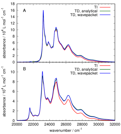
Figure 3: Computed absorption spectra of Coumarin 6 in THF obtained from $\omega$B97x-D/Def2-TZVP calculations. (A) without vibrational pre-excitation, (B) with pre-excitation of the lower-frequency ring mode (see also Fig. 4A). Spectra were computed using the TI approach (red), Fourier transformation of the analytical autocorrelation function (green) and of the wavepacket autocorrelation function (blue). The spectra obtained from the wavepacket propagation have been red-shifted by $90\text{\,}{\mathrm{cm}}^{-1}$ (see text for discussion).

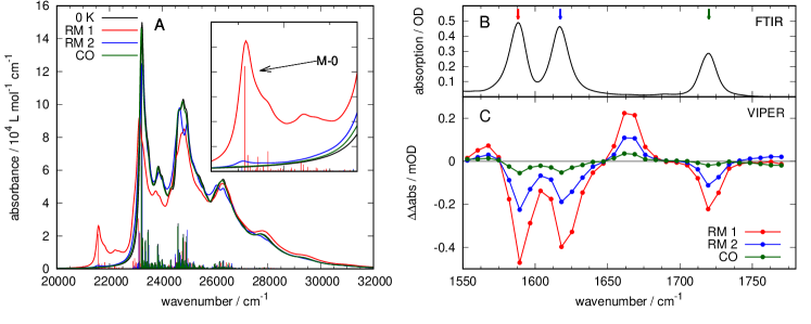
Figure 4: (A) Computed absorption spectra of Coumarin 6 in THF using the analytical TD approach, along with stick spectra obtained from the TI approach, based on a parametrization using $\omega$B97x-D/Def2-TZVP data. Spectra are shown without vibrational pre-excitation (black), with pre-excitation of the lower-frequency ring mode (red), the higher-frequency ring mode (blue) and the CO stretch mode (green). (B) Experimental FTIR absorption spectrum of Coumarin 6 in THF. (C) VIPER spectra of Coumarin 6 in THF after pre-excitation of the lower-frequency ring mode (red), the higher-frequency ring mode (blue) and the CO stretch mode (green). Experimental spectra were recorded using a concentration of 10 mM and a layer thickness of 250 $\mu$m. Details about the experimental set-up can be found in Refs. 2; 1; 3.

V.1 Coumarin 6

Coumarin 6 contains 43 atoms resulting in 123 vibrational normal modes. The most interesting modes in the context outlined above are the carbonyl stretch mode and two ring distortion modes in the coumarin moiety. Coumarin 6 shows a bright HOMO-LUMO transition with $\pi$-$\pi^{*}$ character on the coumarin moiety, exhibiting large oscillator strength.

Figure 3 shows computed absorption spectra of Coumarin 6 at zero temperature in THF, both without vibrational pre-excitation (panel (A)) and with vibrational pre-excitation of the lower-frequency ring mode (panel (B)). Good agreement is obtained between the different methods outlined above. In particular, the analytical TD results and the MCTDH predictions are very close, while the TI approach shows noticeable deviations. The limited convergence of the TI calculations is manifested in some loss of intensity in the high-frequency part of the spectrum. This effect can be attributed to the truncation of the integral calculation, thereby neglecting a large number of very small integrals that are contributing to the high frequency part of the spectrum. For Coumarin 6, $94\text{\,}\mathrm{\char 37\relax}$ of the total spectral intensity are recovered with the chosen number of computed FC integrals, for the spectrum without vibrational pre-excitation. The analytical first moment of the spectrum is $25\,156\text{\,}{\mathrm{cm}}^{-1}$ whereas the resulting TI spectrum has a first moment of $24\,985\text{\,}{\mathrm{cm}}^{-1}$. These results may be improved using higher $N_{\rm max}$ thresholds (see Sec. II.A), at the cost of a significant increase in computational time. It is noteworthy that the convergence of the TI calculations is more challenging in the case of vibrational pre-excitation; this is in line with our previous experience for finite-temperature spectra. For further applications, it is therefore recommended to use the TD approach for a fast and complete calculation of the lineshape, and the TI approach to identify and assign the dominant bands.

The spectra obtained by wavepacket propagation, using ML-MCTDH, feature a somewhat higher total intensity compared to the other methods and are also slightly blue-shifted with a first moment of $25\,392\text{\,}{\mathrm{cm}}^{-1}$. In Fig. 3, this shift has been corrected by $90\text{\,}{\mathrm{cm}}^{-1}$ to show the close agreement of the spectral shape and the detailed features. A slight discrepancy remains, though, due to the different intensity distributions. We attribute the deviation from the analytical TD approach – both in terms of intensity and systematic frequency shifts – to the fact that the ML-MCTDH calculations are not completely converged.

The influence of vibrational pre-excitation on the electronic absorption spectrum of Coumarin 6 is analyzed in further detail in Fig. 4, together with experimental VIPER measurements. In the wavenumber range above $1580\text{\,}{\mathrm{cm}}^{-1}$ only three bands appear, corresponding to two ring modes (labeled RM 1 and RM 2 for the low and high frequency mode, respectively) and one carbonyl stretch mode (labeled CO). In general, vibrational pre-excitation from the global ground state induces additional vibronic transitions upon electronic excitation which have a lower energy than the 0-0-transition. In particular, transitions to the vibrational ground state of the excited electronic state (denoted the M-0-transition) become feasible. These additional transitions induce a red-shift of the low-energy edge of the absorption band. An efficient VIPER excitation requires a high transition probability in this frequency range. In panel (A) of Fig. 4 the M-0 transition after excitation of the lower-frequency ring mode (red) is clearly visible, while the corresponding transitions resulting from excitation of the higher-frequency ring mode and the carbonyl stretch mode are much weaker. This finding is in agreement with the experimental results in panel (C) of Fig. 4, showing the largest VIPER signal upon excitation of the lower-frequency ring mode.

Interestingly, the first moment of the spectrum changes only very slightly upon pre-excitation; in case of the low-frequency ring mode it changes from $25\,156\text{\,}{\mathrm{cm}}^{-1}$ to $25\,082\text{\,}{\mathrm{cm}}^{-1}$. On the other hand, the standard deviation of the spectrum increases from $1744\text{\,}{\mathrm{cm}}^{-1}$ to $2056\text{\,}{\mathrm{cm}}^{-1}$, i. e. the spectrum gets broader while remaining constant in energy. The additional low-frequency transitions are countered by a more pronounced tail in the high frequency range (cf. panel (A) of Fig. 4).

For completeness, we also computed spectra at finite temperature, as documented in Appendix C. These show that the spectral structures are essentially unchanged, indicating that the VIPER excitation will give very similar results at non-zero temperature.

V.2 7-(Diethylamino)coumarin azide (DEACM-N₃)

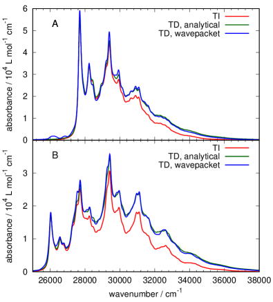
Figure 5: Computed absorption spectra of DEACM-N₃ in acetonitrile obtained from $\omega$B97x-D/Def2-TZVP calculations, (A) without vibrational pre-excitation, (B) with pre-excitation of the lower-frequency ring mode (see also Fig. 6A). The color coding is equivalent to Fig. 3. The spectra obtained from wavepacket propagation has been redshifted by $150\text{\,}{\mathrm{cm}}^{-1}$.

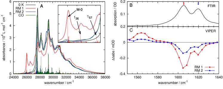
Figure 6: (A) Computed absorption spectra of DEACM-N₃ in acetonitrile using the analytical TD approach, along with stick spectra from the TI approach, based upon $\omega$B97x-D/Def2-TZVP data. Spectra are shown without vibrational pre-excitation (black), with pre-excitation of the lower-frequency ring mode (red), the higher-frequency ring mode (blue) and the CO stretch mode (green). (B) Experimental FTIR absorption spectrum of DEACM-N₃ in acetonitrile. (C) VIPER spectra of DEACM-N₃ in acetonitrile after pre-excitation of the lower-frequency ring mode (red) and the higher-frequency ring mode (blue). Experimental spectra were recorded using a concentration of 25 mM and a layer thickness of 250 $\mu$m.

DEACM-N₃ is also a coumarin derivative, with 102 vibrational modes. Photodissociation of the azide ($N_{3}$) leaving group (“uncaging”) occurs on a picosecond time scalevan Wilderen et al. (2017). The $S_{0}$-$S_{1}$ transition features a pronounced $\pi$-$\pi^{*}$-character and is localized to the coumarin moiety, very similar to Coumarin 6. Due to the structural similarity, vibrational analysis of DEACM-N₃ yields again two distinct ring distortion modes and an intense CO stretch mode in the relevant IR frequency range.

The computed electronic absorption spectrum of DEACM-N₃ is shown in Fig. 5, again without vibrational pre-excitation (panel (A)) and with vibrational pre-excitation of the lower-frequency ring mode (panel (B)). The patterns present in the spectra of Coumarin 6 are also observed in this case. The analytical TD method and the wavepacket approach are again in very good agreement and fully recover the high-frequency part of the spectrum, while the convergence of the TI method is at $88\text{\,}\mathrm{\char 37\relax}$. The first spectral moment has an analytical value of $29\,964\text{\,}{\mathrm{cm}}^{-1}$, for the spectrum without pre-excitation, while the TI method gives a first moment of $29\,642\text{\,}{\mathrm{cm}}^{-1}$. As compared with Coumarin 6, the lack of convergence of the TI approach in the case of vibrational pre-excitation is found to be more pronounced for DEACM-N₃.

The spectrum resulting from the wavepacket propagation is again blueshifted with a first moment of $30\,204\text{\,}{\mathrm{cm}}^{-1}$ and also with a slightly higher intensity. However, the agreement of the features of the spectral lineshape is again very good, except for the spurious intensity below the 0-0 transition. The latter feature, together with the spectral shift and the slight deviations in intensity are most likely due to the incomplete convergence of the ML-MCTDH calculations, as discussed above.

Figure 6 shows the computed absorption spectra of DEACM-N₃ under the influence of vibrational pre-excitation of different modes, together with experimental VIPER measurements. Computations show strong additional redshifted transitions upon excitation of the lower frequency ring mode. In this case the first moment is slightly reduced to $29\,918\text{\,}{\mathrm{cm}}^{-1}$ while the standard deviation increases from $2013\text{\,}{\mathrm{cm}}^{-1}$ to $2488\text{\,}{\mathrm{cm}}^{-1}$. The other modes appear to have a much weaker effect on the spectrum. This observation is consistent with the corresponding results from the calculations on Coumarin 6. This result again supports the experimental findings where the measured VIPER signal has a significantly higher intensity upon pre-excitation of the lower-frequency ring mode compared to the higher-frequency ring mode (see panel (C) of Fig. 6).

V.3 para-Hydroxyphenacyl thiocyanate (pHP-SCN)

The pHP-SCN molecule belongs to the class of para-hydroxy-phenacyl protecting groupsKlán et al. (2012); Park and Givens (1997), with thiocyanate (SCN) as a leaving group. Vibrational analysis of pHP-SCN yields two normal modes (among a total of 54 modes) in the relevant frequency range, both of which are combinations of a ring distortion mode and a carbonyl stretch mode. One of these modes is predominantly of carbonyl stretch type, accompanied by a slight distortion of the ring, and vice versa for the second mode. In both modes, the ring distortion and CO stretch motions are anti-correlated in the sense that an extension (contraction) of the ring distortion coordinate is accompanied by a shortening (lengthening) of the C=O bond.

The lowest singlet excited state of pHP-SCN with non-vanishing oscillator strength corresponds to a $\pi$-$\pi^{*}$-transition in the benzene and carbonyl moiety. The excited-state structure of pHP-SCN posed a significant problem during the search for an excited state minimum. Depending on the choice of density functional and solvation model, extensive state mixing, including exchange of oscillator strength between the state of interest and another, energetically close state, was observed, along with strong distortions of the molecular structure. This is an indication of nonadiabatic coupling between several states – possibly involving triplet statesPark and Givens (1997) – necessitating a treatment with higher-level, multiconfigurational electronic structure methods. In the following, results obtained with the $\omega$B97x-D density functional in THF are reported, which led to a well-defined excited-state minimum structure.

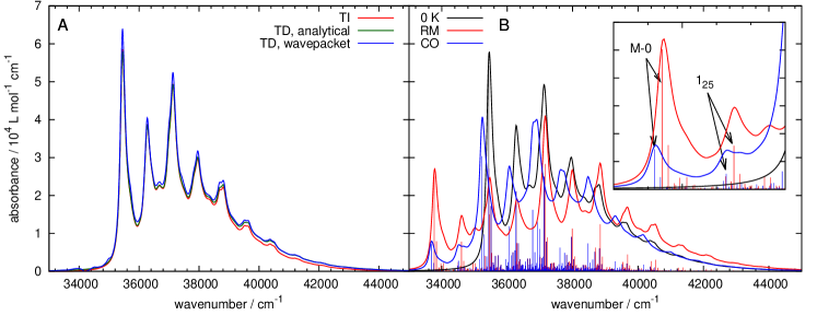
Figure 7: (A) Computed absorption spectra for pHP-SCN in THF obtained from $\omega$B97x-D/Def2-TZVP calculations. The color coding is equivalent to Fig. 3. The spectrum obtained from wavepacket propagation has been redshifted by $45\text{\,}{\mathrm{cm}}^{-1}$. (B) Absorption spectra computed with the analytical autocorrelation function method without vibrational pre-excitation (black), with excitation of the ring distortion mode (red) and the CO stretch mode (blue). Stick spectra from the TI approach are also shown.

Figure 7 shows the computed spectra of pHP-SCN. Since there are no experimental VIPER measurements on pHP-SCN yet, this presents an opportunity to make theoretical predictions. In panel (A) the $0\text{\,}\mathrm{K}$ spectra obtained with the different methods show nearly quantitative agreement. The analytical first moment of the spectrum is $37\,582\text{\,}{\mathrm{cm}}^{-1}$, the TI and wavepacket method yield a value of $37\,508\text{\,}{\mathrm{cm}}^{-1}$ and $37\,726\text{\,}{\mathrm{cm}}^{-1}$, respectively. The TI method is able to recover $98\text{\,}\mathrm{\char 37\relax}$ of the total intensity.

As shown in panel (B) of Fig. 7 vibrational pre-excitation of the ring distortion mode again has the strongest influence on the shape of the spectrum, shifting the analytical first moment to $37\,601\text{\,}{\mathrm{cm}}^{-1}$ while increasing the standard deviation from $1787\text{\,}{\mathrm{cm}}^{-1}$ to $2428\text{\,}{\mathrm{cm}}^{-1}$. However, contrary to the previous examples, the change of the spectrum induced by excitation of the CO stretch mode is non-negligible. In this case, the first moment is $37\,367\text{\,}{\mathrm{cm}}^{-1}$ and the standard deviation is increased to $2080\text{\,}{\mathrm{cm}}^{-1}$.

VI Discussion

The above results for electronic absorption spectra under the influence of vibrational pre-excitation illustrate good agreement between the different computational approaches, and show a pronounced mode-selectivity that is consistent with experiment. Excitation of ring distortion modes induces substantially stronger effects on the spectrum’s low-energy edge than localized stretching modes (e.g. carbonyl modes). These effects can be rationalized by analyzing the ratio of the M-0 to 0-0 transitions (cf. Eq. 36). For the calculations detailed in Section V, the dimensionless displacements $\delta$ and the intensity ratios $S$ are given in Table 1.

Table 1: Dimensionless displacements along the ground state normal modes $\delta_{k}$ and resulting transition intensity ratios $S_{k}$ for the relevant normal modes of the systems investigated here. Data for Coumarin 6 and pHP-SCN is obtained from $\omega$B97x-D/Def2-TZVP calculations in THF while data for DEACM-N₃ results from $\omega$B97x-D/Def2-TZVP calculations in acetonitrile.

	Coumarin 6		DEACM-N3		pHP-SCN
mode	$\delta_{k}$	$S_{k}$	$\delta_{k}$	$S_{k}$	$\delta_{k}$	$S_{k}$
ring mode 1	0.612	0.603	-0.805	-0.809	-0.999	-0.988
ring mode 2	-0.179	-0.131	-0.237	-0.195	—	—
CO stretch	-0.053	-0.043	0.214	0.222	-0.554	-0.528

Overall the correspondence between the values for $S_{k}$ and the observed spectral lineshapes is very good. In the case of Coumarin 6, the lower-frequency ring mode has by far the highest intensity, while the intensity of the higher-frequency ring mode is much lower, and the CO stretch mode mode exhibits negligible intensity (cf. Fig. 4). In the case of DEACM-N₃, the higher-frequency ring mode and the CO stretch mode have comparatively higher intensities which is also reflected in the computed spectra (cf. Fig. 6). In this case the CO stretch mode actually yields a slightly higher intensity than the higher-frequency ring mode. In pHP-SCN the difference between the intensity ratios is not as large as in the coumarin based systems. Here the CO stretch mode appears to be a reasonable choice as a candidate for VIPER excitation. In both coumarin based systems the theoretical predictions agree quite well with the experimental findings regarding the VIPER efficiency of the investigated normal modesvan Wilderen, Messmer, and Bredenbeck (2014); Kern-Michler et al. .

From Eq. 36 it is apparent that $\delta_{k}$ has a strong influence on $S_{k}$. In Table 1, the values for $S$ are indeed very similar to the corresponding $\delta$-values. Additionally, in most cases $S_{k}$ is lower in magnitude than $\delta_{k}$, the only exception being the CO stretch mode of DEACM-N₃. It appears that the displacement of a mode has a much greater influence on its suitability for VIPER excitation than the frequency change and the Duschinsky rotation which are both contributing to the matrix term in Eq. 36.

To further illustrate these points, Figure 8 schematically depicts the vibrational wavefunctions $\ket{\bm{0}_{g}+1_{gk}}$ and $\ket{\bm{0}_{e}}$ whose overlap is critical to the VIPER effect for a simplified model system. Panel (A) shows the simplest case where the modes of the two electronic states coincide. By symmetry the overlap integral $\braket{\bm{0}_{g}+1_{gk}}{\bm{0}_{e}}$ must vanish, even if the frequencies of the excited state modes differ from those of the ground state modes. Therefore, no VIPER transition can occur. Panel (B) shows a corresponding system where the ground state modes are simply rotated with respect to the excited state modes without any displacement. Again, by symmetry the integral vanishes. This can be shown formally by rewriting Eq. 36 using $\bm{J}=\bm{1}$

$$S_{k}=2\delta_{k}\left(1-\frac{\Omega_{gk}}{\Omega_{gk}+\Omega_{ek}}\right)$$ (40)

showing that if $\delta_{k}$ vanishes, so does $S_{k}$. Panel (C) shows a 1D cut of the system of panel (A) along $q_{l}$. Clearly, if no displacement is present, the overlap integral vanishes. In panel (D) a finite displacement between the PESs of the two electronic states is present, leading to a nonzero overlap between the vibrational states, as expressed by Eq. 36.

Figure 8: Schematic illustration of the influence of normal coordinates displacement vs Duschinsky rotation on the overlap of the pre-excited vibrational state $\ket{\bm{0}_{g}+1_{gk}}$ with the vibrational ground state $\ket{\bm{0}_{e}}$. (A) Contour view of the product wavefunction of modes $q_{gk}$ and $q_{gl}$, where $q_{gl}$ has been pre-excited (blue) and the corresponding wavefunction of $q_{ek}$ and $q_{el}$ (red) which represents the vibrational ground state in the excited electronic state. (B) The same but with the ground state modes $q_{gk}$ and $q_{gl}$ rotated w. r. t. their excited state counterparts. Obviously, the overlap is equal in cases (A) and (B). (C) Ground and excited state PES of a pre-excited mode along with the corresponding wavefunctions. The minima of both potentials are coinciding. (D) The same but with a finite displacement between the PESs. Obviously, the overlap is significantly different in cases (C) and (D).

Finally, one should mention that the agreement between the different computational methods is good, but not perfect. Importantly, the spectral features match very well. However, the spectra obtained by wavepacket propagation are consistently blue-shifted relative to their respective analytical counterparts. This effect is likely to result from numerical inaccuracies in energetic offsets, or possibly from the limited convergence of the quantum dynamical propagation due to the finite basis size. In addition, the spectra obtained by wavepacket propagation tend to exhibit spurious structures below the 0-0 transition, which we also attribute to insufficient numerical convergence.

VII Conclusion and outlook

In this work we have presented complementary time-independent and time-dependent approaches for the computation of vibrationally resolved electronic absorption spectra including the effect of pre-excitation of a specific vibrational normal mode. Within the harmonic approximation to the potential energy surfaces, the three methods that were employed – the time-independent FCclasses approach and the time-dependent analytical and numerical wavepacket approaches – formally coincide, and in practice yield good numerical agreement. At this level of treatment, analytical approaches are indeed attractive and efficient alternatives to the more general numerical wavepacket approach (see also Refs. [Huh and Berger, 2011, 2012] for related analytical developments).

In the present context, these methods were applied to three chromophores to investigate their suitability for excitation with the VIPER mixed IR/VIS pulse sequence. We have shown that vibrational pre-excitation leads to an intense M-0 vibronic transition if the equilibrium structure of the excited state features a large displacement along the selected mode with respect to the ground state equilibrium configuration. In this context the role of Duschinsky mixing appears to be less important; in particular a purely rotated vibrational structure without any displacement is shown not to yield any M-0 transitions. The effect of pre-excitation is most pronounced if the electronic transition involves the same structural region of the molecule as the pre-excited normal mode, resulting in a strong vibronic coupling.

Follow-up work will tend to favor the time-dependent approach, in view of including effects of Intramolecular Vibrational Redistribution (IVR) and simulating the full VIPER experiment. While the evaluation of FC integrals and of the analytical autocorrelation function require harmonic PESs, high-dimensional wavepacket propagation is a flexible strategy and can be performed on coupled surfaces line in the case of Linear (LVC) or Quadratic (QVC) Vibronic Coupling modelsKöppel, Domcke, and Cederbaum (2004), and on anharmonic surfaces as well. This opens the road for investigations of both excitations to states exhibiting strong nonadiabatic couplings and the vibrationally hot system’s dynamics on the anharmonic ground state potential energy surface during the time between the IR and the VIS pulse.

Appendix A Derivation of the analytical autocorrelation function

Starting from Eq. 16 of Sec. II.B.1, we introduce an orthogonal transformation to sum and difference coordinates, $\bm{Z}=(\bm{Q}_{e}+\bar{\bm{Q}}_{e})/\sqrt{2},\bm{U}=(\bm{Q}_{e}-\bar{\bm{Q}}_{e})/\sqrt{2}$, to simplify the integrals, in line with Ref. [Baiardi, Bloino, and Barone, 2013]. This results in the following expression for the autocorrelation function,

$$\chi_{k}(t)=2\mu_{0}^{2}\Gamma_{gk}e^{\mathrm{i}(E_{0}/\hbar+\omega_{gk})t} \sqrt{\frac{\det(\bm{\Gamma}_{g})\det(\bm{a}_{e})}{\pi^{N}(2\pi\mathrm{i}\hbar)^{N}}}\exp\left[-\bm{K}^{T}\bm{\Gamma}_{g}\bm{K}\right]\int d\bm{Z}\int d\bm{U}$$ (41)

$$\times\left(K_{k}^{2}+\sqrt{2}K_{k}\sum_{l}J_{kl}Z_{l}+\frac{1}{2}\sum_{l}\sum_{m}J_{kl}J_{km}(Z_{l}+U_{l})(Z_{m}-U_{m})\right)$$

$$\times\exp\left[-\frac{1}{2}\bm{Z}^{T}\bm{D}\bm{Z}-\sqrt{2}\bm{\lambda}^{T}\bm{Z}\right]\exp\left[-\frac{1}{2}\bm{U}^{T}\bm{C}\bm{U}\right]$$

where we used $\bm{\lambda}^{T}:=\bm{K}^{T}\bm{\Gamma}_{g}\bm{J}$ in addition to the definitions of Eq. (II.2.1).

The terms that are linear in $U_{l}$ and $U_{m}$ give no contribution to the integral and can therefore be eliminated. Additionally, the notation can be simplified by defining the vector $\bm{\alpha}^{(k)}$ with $\alpha^{(k)}_{l}=J_{kl}$ and the matrix $\bm{\beta}^{(k)}$ with $\beta^{(k)}_{lm}=J_{kl}J_{km}$:

$$\chi_{k}(t)=2\mu_{0}^{2}\Gamma_{gk}e^{\mathrm{i}(E_{0}/\hbar+\omega_{gk})t} \sqrt{\frac{\det(\bm{\Gamma}_{g})\det(\bm{a}_{f})}{\pi^{N}(2\pi\mathrm{i}\hbar)^{N}}}\exp\left[-\bm{K}^{T}\bm{\Gamma}_{g}\bm{K}\right]\int d\bm{Z}\int d\bm{U}$$ (42)

$$\times\left(K_{k}^{2}+\sqrt{2}K_{k}\left(\bm{\alpha}^{(k)}\right)^{T}\bm{Z}+\frac{1}{2}\bm{Z}^{T}\bm{\beta}^{(k)}\bm{Z}-\frac{1}{2}\bm{U}^{T}\bm{\beta}^{(k)}\bm{U}\right)$$

$$\times\exp\left[-\frac{1}{2}\bm{Z}^{T}\bm{D}\bm{Z}-\sqrt{2}\bm{\lambda}^{T}\bm{Z}\right]\exp\left[-\frac{1}{2}\bm{U}^{T}\bm{C}\bm{U}\right]$$

Before proceeding, we simplify the prefactor by using

$$e^{\mathrm{i}\frac{E_{0}}{\hbar}t}=\prod_{k}e^{\mathrm{i}\frac{\hbar}{2}\Gamma_{gk}t}=\det\left(e^{\mathrm{i}\frac{\hbar}{2}\bm{\Gamma}_{g}t}\right)=\sqrt{\frac{1}{\det\left(e^{-\mathrm{i}\hbar\bm{\Gamma}_{g}t}\right)}}\qquad\text{and}\qquad\bm{a}^{\prime}_{g}(t)=\frac{2\mathrm{i}\hbar\bm{\Gamma}_{g}}{e^{-\mathrm{i}\hbar\bm{\Gamma}_{g}t}}$$ (43)

and split the autocorrelation function into three components:

$$\chi_{k}(t)=2\Gamma_{gk}e^{\mathrm{i}\hbar\Gamma_{gk}t}\left[K_{k}^{2}\chi^{0}_{FC}(t)+K_{k}\chi^{0}_{k,a}(t)+\chi^{0}_{k,b}(t)\right]$$ (44)

with

$$\chi^{0}_{FC}(t)=\mu_{0}^{2}\sqrt{\frac{\det(\bm{a}^{\prime}_{g}(t)\bm{a}_{e}(t))}{(2\pi\mathrm{i}\hbar)^{2N}}}\exp\left[-\bm{K}^{T}\bm{\Gamma}_{g}\bm{K}\right]\int d\bm{Z}\int d\bm{U}\exp\left[-\frac{1}{2}\bm{Z}^{T}\bm{D}\bm{Z}-\sqrt{2}\bm{\lambda}^{T}\bm{Z}\right]\exp\left[-\frac{1}{2}\bm{U}^{T}\bm{C}\bm{U}\right]$$ (45)

$$\chi^{0}_{k,a}(t)=\sqrt{2}\mu_{0}^{2}\sqrt{\frac{\det(\bm{a}^{\prime}_{g}(t)\bm{a}_{e}(t))}{(2\pi\mathrm{i}\hbar)^{2N}}}\exp\left[-\bm{K}^{T}\bm{\Gamma}_{g}\bm{K}\right]\int d\bm{Z}\int d\bm{U}\left(\bm{\alpha}^{(k)}\right)^{T}\bm{Z}$$ (46)

$$\exp\left[-\frac{1}{2}\bm{Z}^{T}\bm{D}\bm{Z}-\sqrt{2}\bm{\lambda}^{T}\bm{Z}\right]\exp\left[-\frac{1}{2}\bm{U}^{T}\bm{C}\bm{U}\right]$$

$$\chi^{0}_{k,b}(t)=\frac{1}{2}\mu_{0}^{2}\sqrt{\frac{\det(\bm{a}^{\prime}_{g}(t)\bm{a}_{e}(t))}{(2\pi\mathrm{i}\hbar)^{2N}}}\exp\left[-\bm{K}^{T}\bm{\Gamma}_{g}\bm{K}\right]\int d\bm{Z}\int d\bm{U}\left(\bm{Z}^{T}\bm{\beta}^{(k)}\bm{Z}-\bm{U}^{T}\bm{\beta}^{(k)}\bm{U}\right)$$ (47)

$$\exp\left[-\frac{1}{2}\bm{Z}^{T}\bm{D}\bm{Z}-\sqrt{2}\bm{\lambda}^{T}\bm{Z}\right]\exp\left[-\frac{1}{2}\bm{U}^{T}\bm{C}\bm{U}\right]$$

where $\chi^{0}_{FC}(t)$ is the FC correlation function at $0\text{\,}\mathrm{K}$ while $\chi^{0}_{k,a}(t)$ and $\chi^{0}_{k,b}(t)$ are analogous to mixed Franck-Condon/Herzberg-Teller and Herzberg-Teller terms, respectivelyBaiardi, Bloino, and Barone (2013). The integrals in Eq. 45 can be solved by using the substitutions $\bm{Z}_{1}=\bm{D}^{1/2}\bm{Z}+\sqrt{2}\bm{D}^{1/2}\bm{\lambda}$ and $\bm{U}_{1}=\bm{C}^{1/2}\bm{U}$, resulting in

$$\chi^{0}_{FC}(t)=\mu_{0}^{2}\sqrt{\frac{\det(\bm{a}^{\prime}_{g}(t)\bm{a}_{e}(t))}{(2\pi\mathrm{i}\hbar)^{2N}\det(\bm{CD})}}\exp\left[-\bm{K}^{T}\bm{\Gamma}_{g}\bm{K}\right]\exp\left[\bm{\lambda}^{T}\bm{D}^{-1}\bm{\lambda}\right]\int d\bm{Z}_{1}\exp\left[-\frac{1}{2}\bm{Z}_{1}^{T}\bm{Z}_{1}\right]\int d\bm{U}_{1}\exp\left[-\frac{1}{2}\bm{U}_{1}^{T}\bm{U}_{1}\right]$$ (48)

where the Gaussian integrals are known:

$$\int d\bm{Z}_{1}\exp\left[-\frac{1}{2}\bm{Z}_{1}^{T}\bm{Z}_{1}\right]=\int d\bm{U}_{1}\exp\left[-\frac{1}{2}\bm{U}_{1}^{T}\bm{U}_{1}\right]=(2\pi)^{N/2}$$ (49)

So we finally arrive at

$$\chi^{0}_{FC}(t)=\mu_{0}^{2}\sqrt{\frac{\det(\bm{a}^{\prime}_{g}(t)\bm{a}_{e}(t))}{(\mathrm{i}\hbar)^{2N}\det(\bm{CD})}}\exp\left[-\bm{K}^{T}\bm{\Gamma}_{g}\bm{K}+\bm{\lambda}^{T}\bm{D}^{-1}\bm{\lambda}\right].$$ (50)

The same technique can be applied to the integrals in Eqs. 46 and 47 to obtain

$$\chi^{0}_{k,a}(t)=-2\chi^{0}_{FC}(t)\left(\bm{\alpha}^{(k)}\right)^{T}\bm{D}^{-1}\bm{\lambda}$$ (51)

and

$$\chi^{0}_{k,b}(t)=\frac{1}{2}\chi^{0}_{FC}(t) \left(2\bm{\lambda}^{T}\bm{D}^{-1}\bm{\beta}^{(k)}\bm{D}^{-1}\bm{\lambda}\right.$$ (52)

$$\left.+\mathrm{Tr}[\bm{\beta}^{(k)}(\bm{D}^{-1}-\bm{C}^{-1})]\right)$$

The above expression is equivalent to Eq. (18) of the main text, when taking into account the additional definitions specified in Section II.2.1.

Appendix B Construction of the ML-MCTDH tree

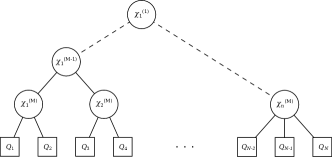
Figure 9: Schematic representation of the multilayer tree structure where $N$ normal modes are arranged into $M$ layers.

Within the ML-MCTDH framework, the wavefunction is defined in terms of a tree structure consisting of combinations of single-particle functions (SPFs). In Fig. 9, the structure of the multi-layer tree is illustrated. The tree was constructed by first ordering the normal modes with increasing frequency. Typically, $M=6$ layers were employed, with the number of SPFs varying from $n_{\rm SPF}$=3 to $n_{\rm SPF}$=8 SPFs per subspace in each layer. In the last layer, the single-particle functions are represented by a harmonic-oscillator (HO) Discrete-Variable Representation (DVR) with 10-20 DVR points.

The lowest-layer particles were built by combining adjacent pairs of normal modes into one particle, creating two-dimensional subspaces. If the total number of normal modes is odd, the last particle contains three modes instead of two. The lowest-level particles are then again combined pairwise, forming the particles of the next higher layer. This process is continued until only two or three particles remain, which then constitute the top layer.

Appendix C Spectra at finite temperature

Our treatment of the VIPER excitation assumes a $0\text{\,}\mathrm{K}$ initial state because the frequencies of the vibrational modes that are involved in the vibrational pre-excitation are much higher than $kT$ at room temperature. Nonetheless, spectra at finite temperature were computed, using the analytic TD approachSantoro and Lami (2012); Avila Ferrer et al. (2014); Baiardi, Bloino, and Barone (2013); Ianconescu and Pollak (2004); Tatchen and Pollak (2008); Tang, Lee, and Lin (2003); Yan and Mukamel (1986); Mukamel, Abe, and Islampour (1985); Kubo and Toyozawa (1955); Huh and Berger (2012); Baiardi, Bloino, and Barone (2014), to check whether these spectra are simply broadened with respect to the zero-temperature case, or whether any additional vibronic transitions from excited vibrational states arise. Figure 10 shows computed absorption spectra of Coumarin 6 confirming that increasing the temperature simply leads to a broadening of the vibronic fine-structure and no additional lower-energy transitions are observed.

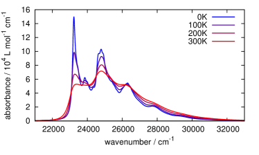
Figure 10: Computed spectra of Coumarin 6 in THF at different temperatures obtained from $\omega$B97x-D/Def2-TZVP calculations using the analytic autocorrelation function approach.

References

- van Wilderen and Bredenbeck (2015) L. J. G. W. van Wilderen and J. Bredenbeck, Angew. Chem. Int. Ed. 54, 11624 (2015).
- van Wilderen, Messmer, and Bredenbeck (2014) L. J. G. W. van Wilderen, A. T. Messmer, and J. Bredenbeck, Angew. Chem. Int. Ed. 53, 2667 (2014).
- (3) D. Kern-Michler, C. Neumann, N. Mielke, L. J. G. W. van Wilderen, M. Reinfelds, J. von Cosel, A. Heckel, I. Burghardt, and J. Bredenbeck, In preparation.
- Klán et al. (2012) P. Klán, T. Šolomek, C. G. Bochet, A. Blanc, R. Givens, M. Rubina, V. Popik, A. Kostikov, and J. Wirz, Chem. Rev. 113, 119 (2012).
- Park and Givens (1997) C. Park and R. Givens, J. Am. Chem. Soc. 119, 2453 (1997).
- van Wilderen et al. (2017) L. J. G. W. van Wilderen, C. Neumann, A. Rodrigues-Correia, D. Kern-Michler, N. Mielke, M. Reinfelds, A. Heckel, and J. Bredenbeck, Phys. Chem. Chem. Phys. 19, 6487 (2017).
- Santoro et al. (2007a) F. Santoro, R. Improta, A. Lami, J. Bloino, and V. Barone, J. Chem. Phys. 126, 084509 (2007a).
- Santoro et al. (2007b) F. Santoro, A. Lami, R. Improta, and V. Barone, J. Chem. Phys. 126, 184102 (2007b).
- Santoro et al. (2008) F. Santoro, A. Lami, R. Improta, J. Bloino, and V. Barone, J. Chem. Phys. 128, 224311 (2008).
- Wang and Thoss (2003) H. Wang and M. Thoss, J. Chem. Phys. 119, 1289 (2003).
- Vendrell and Meyer (2011) O. Vendrell and H.-D. Meyer, J. Chem. Phys. 134, 044135 (2011).
- Meyer, Manthe, and Cederbaum (1990) H.-D. Meyer, U. Manthe, and L. S. Cederbaum, Chem. Phys. Lett. 165, 73 (1990).
- Beck et al. (2000) M. H. Beck, A. Jäckle, G. A. Worth, and H.-D. Meyer, Phys. Rep. 324, 1 (2000).
- Worth et al. (2008) G. A. Worth, H.-D. Meyer, H. Köppel, L. S. Cederbaum, and I. Burghardt, Int. Rev. Phys. Chem. 27, 569 (2008).
- Duschinsky (1937) F. Duschinsky, Acta Physicochim. U. R. S. S. 7, 551 (1937).
- Tannor (2007) D. J. Tannor, Introduction to quantum mechanics: A time-dependent perspective, 1st ed. (University Science Books, USA, 2007).
- (17) F. Santoro, “FCClasses, a Fortran 77 code,” Available at http://village.pi.iccom.cnr.it/Software.
- Santoro and Lami (2012) F. Santoro and A. Lami, in Computational Strategies for Spectroscopy: From Small Molecules to Nano Systems, edited by V. Barone (John Wiley & Sons, Inc., 2012) Chap. 10, pp. 475–516.
- Avila Ferrer et al. (2014) F. J. Avila Ferrer, J. Cerezo, J. Soto, R. Improta, and F. Santoro, Comput. Theor. Chem. 1040–1041, 328 (2014).
- Baiardi, Bloino, and Barone (2013) A. Baiardi, J. Bloino, and V. Barone, J. Chem. Theory Comput. 9, 4097 (2013).
- Ianconescu and Pollak (2004) E. Ianconescu and E. Pollak, J. Phys. Chem. A 108, 7778 (2004).
- Tatchen and Pollak (2008) J. Tatchen and E. Pollak, J. Chem. Phys. 128, 164303 (2008).
- Tang, Lee, and Lin (2003) J. Tang, M. T. Lee, and S. H. Lin, J. Chem. Phys. 119, 7188 (2003).
- Yan and Mukamel (1986) Y. Yan and S. Mukamel, J. Chem. Phys. 85, 5908 (1986).
- Mukamel, Abe, and Islampour (1985) S. Mukamel, S. Abe, and R. Islampour, J. Phys. Chem. 89, 201 (1985).
- Kubo and Toyozawa (1955) R. Kubo and Y. Toyozawa, Prog. Theor. Phys. 13, 160 (1955).
- Huh and Berger (2012) J. Huh and R. Berger, J. Phys. Conf. Ser. 380, 012019 (2012).
- Baiardi, Bloino, and Barone (2014) A. Baiardi, J. Bloino, and V. Barone, J. Chem. Phys. 141, 114108 (2014).
- Peng et al. (2010) Q. Peng, Y. Niu, C. Deng, and Z. Shuai, Chem. Phys. 370, 215 (2010).
- Borrelli, Capobianco, and Peluso (2012) R. Borrelli, A. Capobianco, and A. Peluso, J. Phys. Chem. A 116, 9934 (2012).
- Biczysko et al. (2012) M. Biczysko, J. Bloino, F. Santoro, and V. Barone, in Computational Strategies for Spectroscopy: From Small Molecules to Nano Systems, edited by V. Barone (John Wiley & Sons, Inc., 2012) Chap. 8, pp. 361–443.
- Mukamel (1999) S. Mukamel, Principles of Nonlinear Optical Spectroscopy, 1st ed. (Oxford University Press, Oxford, 1999).
- Frisch et al. (2013) M. J. Frisch, G. W. Trucks, H. B. Schlegel, G. E. Scuseria, M. A. Robb, J. R. Cheeseman, G. Scalmani, V. Barone, B. Mennucci, G. A. Petersson, H. Nakatsuji, M. Caricato, X. Li, H. P. Hratchian, A. F. Izmaylov, J. Bloino, G. Zheng, J. L. Sonnenberg, M. Hada, M. Ehara, K. Toyota, R. Fukuda, J. Hasegawa, M. Ishida, T. Nakajima, Y. Honda, O. Kitao, H. Nakai, T. Vreven, J. A. Montgomery, Jr., J. E. Peralta, F. Ogliaro, M. Bearpark, J. J. Heyd, E. Brothers, K. N. Kudin, V. N. Staroverov, R. Kobayashi, J. Normand, K. Raghavachari, A. Rendell, J. C. Burant, S. S. Iyengar, J. Tomasi, M. Cossi, N. Rega, J. M. Millam, M. Klene, J. E. Knox, J. B. Cross, V. Bakken, C. Adamo, J. Jaramillo, R. Gomperts, R. E. Stratmann, O. Yazyev, A. J. Austin, R. Cammi, C. Pomelli, J. W. Ochterski, R. L. Martin, K. Morokuma, V. G. Zakrzewski, G. A. Voth, P. Salvador, J. J. Dannenberg, S. Dapprich, A. D. Daniels, Ö. Farkas, J. B. Foresman, J. V. Ortiz, J. Cioslowski, and D. J. Fox, “Gaussian 09 Revision D.01,” (2013), Gaussian Inc. Wallingford CT.
- Chai and Head-Gordon (2008) J.-D. Chai and M. Head-Gordon, Phys. Chem. Chem. Phys. 10, 6615 (2008).
- Yanai, Tew, and Handy (2004) T. Yanai, D. P. Tew, and N. C. Handy, Chem. Phys. Lett. 393, 51 (2004).
- Adamo and Barone (1999) C. Adamo and V. Barone, J. Chem. Phys. 110, 6158 (1999).
- Weigend and Ahlrichs (2005) F. Weigend and R. Ahlrichs, Phys. Chem. Chem. Phys. 7, 3297 (2005).
- Ferrer and Santoro (2012) F. J. A. Ferrer and F. Santoro, Phys. Chem. Chem. Phys. 14, 13549 (2012).
- (39) G. A. Worth, M. H. Beck, A. Jäckle, O. Vendrell, and H.-D. Meyer, The MCTDH Package, Version 8.5.4 See http://mctdh.uni-hd.de/.
- Press et al. (2007) W. H. Press, S. A. Teukolsky, W. T. Vetterling, and B. P. Flannery, Numerical Recipes 3rd Edition: The Art of Scientific Computing, 3rd ed. (Cambridge University Press, New York, NY, USA, 2007).
- Huh and Berger (2011) J. Huh and R. Berger, Faraday Discuss. 150, 363 (2011).
- Köppel, Domcke, and Cederbaum (2004) H. Köppel, W. Domcke, and L. S. Cederbaum, in Conical Intersections, edited by W. Domcke, D. R. Yarkony, and H. Köppel (World Scientific Co., 2004) pp. 323–368.