On the mass and luminosity functions of tidal disruption flares:
rate suppression due to black hole event horizons
Abstract
The tidal disruption of a star by a massive black hole is expected to yield a luminous flare of thermal emission. About two dozen of these stellar tidal disruption flares (TDFs) may have been detected in optical transient surveys. However, explaining the observed properties of these events within the tidal disruption paradigm is not yet possible. This theoretical ambiguity has led some authors to suggest that optical TDFs are due to a different process, such as a nuclear supernova or accretion disk instabilities. Here we present a test of a fundamental prediction of the tidal disruption event scenario: a suppression of the flare rate due to the direct capture of stars by the black hole. Using a recently compiled sample of candidate TDFs with black hole mass measurements, plus a careful treatment of selection effects in this flux-limited sample, we confirm that the dearth of observed TDFs from high-mass black holes is statistically significant. All the TDF impostor models we consider fail to explain the observed mass function; the only scenario that fits the data is a suppression of the rate due to direct captures. We find that this suppression can explain the low volumetric rate of the luminous TDF candidate ASASSN-15lh, thus supporting the hypothesis that this flare belongs to the TDF family. Our work is the first to present the optical TDF luminosity function. A steep power law is required to explain the observed rest-frame -band luminosity, . The mean event rate of the flares in our sample is galaxy-1 yr-1, consistent with the theoretically expected tidal disruption rate.
1. Introduction
A stellar tidal disruption event (TDE) happens when a star passes within the Roche radius of a massive black hole. As the streams of stellar debris circularize and are accreted by the black hole, we can expect a luminous flare of thermal emission (Rees, 1988). The first (candidates) of these stellar tidal disruption flares (TDFs) were discovered with X-ray surveys (Bade et al., 1996; Komossa & Bade, 1999), followed by UV-selected flares (Gezari et al., 2006, 2009). The detection of new TDFs is currently dominated by optical surveys (van Velzen et al., 2011; Gezari et al., 2012; Arcavi et al., 2014; Holoien et al., 2014). About two new candidates are found each year, and this number is certain to increase in the near future as larger optical surveys (ZTF, LSST) become operational.
Stellar tidal disruption flares can be considered a multipurpose tool for extragalactic astrophysics. First of all, they can be used as probes to signal the existence of black holes in quiescent galaxies, potentially including intermediate-mass black holes in dwarf galaxies (Maksym et al., 2013; MacLeod et al., 2014). The dynamics of the TDE itself are also interesting; the rapid increase of the fallback rate of the stellar debris (from super- to sub-Eddington in a few years) presents a new domain to test our understanding of accretion physics. In particular, the detection of radio emission following TDFs (Zauderer et al., 2011; Bloom et al., 2011; Levan et al., 2011; van Velzen et al., 2016b; Alexander et al., 2017) can shed new light on the conditions required for the launch of relativistic jets.
While TDFs appear to be promising tools, their optical emission has proven to be difficult to model self-consistently. The observed temperature is too low to originate from a compact accretion disk near the pericenter of the stellar orbit (Strubbe & Quataert, 2011; Lodato & Rossi, 2011; van Velzen et al., 2011). Reprocessing of high-energy photons from the compact accretion disk by material at larger radii (Guillochon et al., 2014; Metzger & Stone, 2016) and emission due to shocks caused by intersecting debris streams (Piran et al., 2015; Krolik et al., 2016) have both been proposed as explanations for optical TDF emission. Neither explanation is completely satisfactory. The intersecting-stream scenario suffers from a “missing energy problem” (Piran et al., 2015), whereas the reprocessing scenario appears at odds with the (tentative) discovery that the X-ray emission lags the UV emission (Pasham et al., 2017).
Contrary to the optical emission, the X-ray properties of TDF candidates generally fit within the canonical TDE picture of Rees (1988); see Komossa (2015); Auchettl et al. (2017a) for reviews. Since very few X-ray selected TDFs have received optical follow-up near peak (Saxton et al., 2017), it could be possible that X-ray-selected and optically selected TDF candidates are a separate class of tidal disruptions (Dai et al., 2015). Some authors have gone one step further and proposed that most optically selected TDF candidates are, in fact, not due to the tidal disruption of a star. Supernovae (SNe) in AGN accretion disks (Saxton et al., 2016), collisions of stars on bound orbits around the black hole (Metzger & Stone, 2017), black hole accretion disk instabilities (Saxton et al., 2016), or flares from accreting supermassive black hole binaries with subparsec separations (Tanaka, 2013) have been proposed as potential TDF impostors.
The hypothesis that flares from active galactic nuclei (AGN) are TDF impostors perhaps has the most observational support because relatively rapid changes of AGN luminosity and spectral type have been observed (Storchi-Bergmann et al., 1993; Shappee et al., 2014; LaMassa et al., 2015; Gezari et al., 2017). While the observed properties of these changing-look AGN are different from candidate TDFs (Ruan et al., 2016; MacLeod et al., 2016), their existence demonstrates that the luminosity of AGN can increase beyond what is expected from the power spectrum that accurately describes the light curves of mundane AGN (MacLeod et al., 2012; Graham et al., 2017).
The mechanism that triggers the accretion rate increase in changing-look AGN could be similar to the thermal-viscous instability (Meyer & Meyer-Hofmeister, 1981; Smak, 1983) that is known to operate in disks around stellar-mass compact objects that accrete from a donor star (van Paradijs, 1996; Lasota, 2001). For black holes with a mass of , a similar mechanism (Mineshige & Shields, 1990; Siemiginowska & Elvis, 1997; Janiuk et al., 2002) could lead to outbursts with a recurrence time of (Hatziminaoglou et al., 2001; Czerny et al., 2009). However, Hameury, Viallet, & Lasota (2009) argue that due to the high Mach number in AGN accretion disks, this quiescent time could be much shorter, and therefore large outbursts due to limit-cycle oscillations may not be expected for AGN.
The tidal disruption of a star can also occur in a Seyfert galaxy (e.g., Drake et al., 2011; Blanchard et al., 2017)—perhaps such events could explain some of the changing-look AGN (Merloni et al., 2015; Wyrzykowski et al., 2017). Identifying observations that can discriminate between an AGN disk instability triggered by a star passing through the disk and a TDE inside a galaxy that also harbors an AGN is very challenging; these events are a mix of two phenomena that are not yet completely understood even if they occur in isolation. Fortunately, we can largely avoid this problem if we consider only TDF candidates from galaxies that are not classified as AGN before the optical outburst.
One signature is unique to a TDE and can thus be used to rule out most—or perhaps all—TDF impostor scenarios. A TDE requires that the star passes within the tidal radius,
| (1) |
Here we expressed the tidal radius for a solar-type star in units of the Schwarzschild radius (). For a black hole mass of the tidal radius of a solar-type star is equal to the Schwarzschild radius, and the results of the disruption will not be visible to an observer outside the black hole event horizon (Hills, 1975). This critical black hole mass is sometimes referred to as the Hills mass.
Repeating the calculation behind Eq. 1 within in the framework of General Relativity, one finds that the Hills mass increases with black hole spin (Kesden, 2012). For spinning black holes, the outcome of the disruption also depends on the orientation between the black hole angular momentum vector and the star’s orbital plane; after averaging over all inclinations, Kesden (2012) finds that the effect of the black hole horizon yields a superexponential suppression of the TDF rate for .
The goal of this work is to use the expected suppression in the flare rate due to a black hole horizon to demonstrate that optically selected TDF candidates are indeed due to the tidal disruption of a star.
The outline of this paper is as follows. We will first present our compilation of TDF candidates in Sec. 2. Next, we compute the luminosity function (LF) and host galaxy mass function for this sample (Sec. 3). We then use forward modeling to reproduce the observed distribution of black hole mass and galaxy mass (Sec. 4). We discuss the implications of this result (Sec. 5) and close with a list of conclusions (Sec. 6). We adopt a flat cosmology with and . All magnitudes are in the AB (Oke, 1974) system.
1.1. TDE or TDF?
In the literature, both tidal disruption event (TDE) and tidal disruption flare (TDF) are used to label transients due to stellar disruptions. In this work, we use TDE to refer to the general concept of the disruption of a star by a black hole, while TDF is used only for the electromagnetic result of this disruption. This distinction is subtle, yet useful, since not every TDE may lead to a TDF (e.g., Guillochon & Ramirez-Ruiz, 2015).
| name | R.A. | Decl. | ||||||
|---|---|---|---|---|---|---|---|---|
| (J2000) | (J2000) | ( | ( K) | ( | ||||
| GALEX-D1-9 | 02:25:16.96 | 04:32:59.1 | 22.4 (NUV) | 5.6 | 44.1 | 0.326 | 0.554 | |
| GALEX-D3-13 | 14:19:29.78 | 52:52:06.3 | 22.2 (NUV)∗ | 4.9 | 44.3 | 0.370 | 0.821 | |
| GALEX-D23H-1 | 23:31:59.53 | 00:17:14.5 | 20.9 (NUV) | 4.9 | 43.9 | 0.185 | 0.517 | |
| SDSS-TDE1 | 23:42:01.40 | 01:06:29.2 | 21.0 ()∗ | 2.4 | 43.5 | 0.136 | 0.174 | |
| SDSS-TDE2 | 23:23:48.61 | 01:08:10.2 | 20.3 ()∗ | 1.8 | 44.0 | 0.256 | 0.469 | |
| PS1-10jh | 16:09:28.27 | 53:40:23.9 | 19.8 () | 2.9 | 44.2 | 0.170 | 0.409 | |
| PS1-11af | 09:57:26.81 | 03:14:00.9 | 21.4 () | 1.9 | 43.9 | 0.405 | 0.426 | |
| PTF-09ge | 14:57:03.18 | 49:36:40.9 | 17.7 () | 2.2 | 44.1 | 0.064 | 0.155 | |
| PTF-09axc | 14:53:13.07 | 22:14:32.2 | 19.1 () | 1.2 | 43.5 | 0.115 | 0.138 | |
| PTF-09djl | 16:33:55.97 | 30:14:16.6 | 19.6 () | 2.6 | 44.4 | 0.184 | 0.179 | |
| ASASSN-14ae | 11:08:40.11 | 34:05:52.2 | 17.0 ()∗ | 2.1 | 43.9 | 0.044 | 0.051 | |
| ASASSN-14li | 12:48:15.23 | 17:46:26.4 | 16.8 ()∗ | 3.5 | 43.8 | 0.021 | 0.025 | |
| ASASSN-15oi | 20:39:09.14 | 30:45:20.6 | 16.2 ()∗ | 2.5 | 44.4 | 0.048 | 0.082 | |
| ASASSN-15lh | 22:02:15.44 | 61:39:34.5 | 16.5 () | 2.5 | 45.6 | 0.233 | 0.347 | |
| iPTF-15af | 08:48:28.13 | 22:03:33.4 | – | – | – | – | 0.079 | 0.101 |
| iPTF-16axa | 17:03:34.34 | 30:35:36.6 | 18.5 ()∗ | 3.0 | 44.5 | 0.108 | 0.135 | |
| iPTF-16fnl | 00:29:57.05 | 32:53:37.2 | 17.4 () | 3.0 | 43.4 | 0.016 | 0.034 |
Note. — The third column, , lists the maximum observed apparent magnitude and the relevant filter for each survey; an asterisk indicates that the peak of the light curve was not resolved. The forth and fifth columns give the rest-frame -band luminosity, as computed using the observed blackbody temperature () to make the k-correction. The last column lists the maximum redshift where this flare could have been detected given the survey effective flux limit.
| name | gal. mass | ||||||||
|---|---|---|---|---|---|---|---|---|---|
| (km s | |||||||||
| GALEX-D1-9 | 10.3 | 0.324 | |||||||
| GALEX-D3-13 | 10.7 | 0.375 | |||||||
| GALEX-D23H-1 | 10.3 | 0.395 | |||||||
| SDSS-TDE1 | 10.1 | 0.275 | |||||||
| SDSS-TDE2 | 10.6 | 0.410 | |||||||
| PS1-10jh | 9.5 | 0.170 | |||||||
| PS1-11af | 10.1 | 0.284 | |||||||
| PTF-09ge | 10.1 | 0.330 | |||||||
| PTF-09axc | 10.0 | 0.411 | |||||||
| PTF-09djl | 10.1 | 0.323 | |||||||
| ASASSN-14ae | 9.8 | 0.291 | |||||||
| ASASSN-14li | 9.6 | 0.249 | |||||||
| ASASSN-15oi | 9.9 | 0.301 | |||||||
| ASASSN-15lh | 10.8 | 0.571 | |||||||
| iPTF-15af | 10.2 | 0.341 | |||||||
| iPTF-16axa | 10.1 | 0.314 | |||||||
| iPTF-16fnl | 9.8 | 0.277 |
Note. — The apparent magnitudes (, , and ) are corrected for Galactic extinction using the Schlafly & Finkbeiner (2011) extinction maps. Uncertainties on the apparent magnitudes include only the statistical uncertainty. The absolute magnitudes are computed in the rest frame of the host galaxy. The total stellar mass of the galaxy is estimated from the broadband (ugrizJHK) photometry. The velocity dispersion () measurements are from the sample of Wevers et al. (2017) (with the exception of ASASSN-15lh). The last column lists the maximum redshift for inclusion of the galaxy in the Wevers et al. (2017) sample.
2. Observed TDFs
We will restrict our sample of candidate TDFs to nuclear flares found in optical/UV imaging surveys. The first motivation for this choice is the fact that candidate TDFs from optical imaging surveys show a number of common properties (discussed below), which justifies treating these flares as one class in our analysis. Further motivation for restricting to optical surveys is that other methods to find TDFs, X-ray surveys, or extreme coronal line emitters in spectroscopic galaxy samples (Komossa et al., 2008) require more assumptions to estimate the event rate. For these surveys, the cadence is (much) lower than the duration of the flare and estimating the volumetric flare rate requires a light-curve model (or one could measure the snapshot rate; see Auchettl, Ramirez-Ruiz, & Guillochon 2017b).
We exclude flares found in galaxies that can be classified as a broad-line AGN or Seyfert, but we include flares from LINERs (Heckman, 1980), leaving 17 sources (Table 1). Our selection requirements and final sample are similar to the candidate TDF samples presented recently (Hung et al., 2017; Wevers et al., 2017). The only difference is that this earlier work used stricter requirements on either the TDF light-curve sampling (to be able to measure the decay rate) or the host brightness and Declination (to allow efficient spectroscopic follow-up).
These 17 flares share a number of properties: a high blackbody temperature ( K) and nearly constant colors (e.g., Hung et al. 2017, Fig. 11). Also the optival/UV light curves of the TDFs in our sample are all consistent with a power-law decay rate; in all cases where monitoring observations cover more than one year of the light curve, an exponential decay rate can be ruled out (van Velzen et al., 2011; Arcavi et al., 2014; Gezari et al., 2015; van Velzen et al., 2016b; Brown et al., 2016, 2017).
In Table 1 we summarize the observed properties of the flares in our sample. To measure the rest-frame -band luminosity () we used the observed blackbody luminosity to compute the k-correction (Hogg et al., 2002).
| Survey | band | ||||
|---|---|---|---|---|---|
| (deg2 yr) | |||||
| GALEX | 3 | 23.0 | NUV | 0.393 | 17 |
| SDSS | 2 | 21.5 | r | 0.140 | 202 |
| PS1 | 2 | 21.5 | g | 0.168 | 120 |
| PTF | 3 | 19.5 | r | 0.054 | 3000 |
| iPTF | 3 | 19.5 | r | 0.054 | 5032 |
| ASAS-SN | 4 | 17.3 | g | 0.023 | 82637 |
Note. — The second column lists the number of candidate TDFs from each survey. The typical maximum redshift for each survey () follows from the requirement that a flare with a peak luminosity of is detectable above the effective flux limit (). From this redshift we can compute (Eq. 2) the effective area times the survey duration.
Measurements of the velocity dispersion of the host galaxy have been obtained by Wevers et al. (2017) for 12 of the 17 TDFs in our sample. This sample includes only sources at Declination and is complete for a host galaxy flux limit of and .
The stellar mass of the TDF host galaxies is estimated from broadband optical to near-IR photometry using correct \citep{blanton07}. The same software and wavelength range was used to estimate the mass of galaxies that are input for our synthetic sample of potential TDF host galaxies (see Sec.~\ref{sec:moc). We use the SDSS (York et al., 2000) Petrosian (Blanton et al., 2001; Stoughton et al., 2002) magnitudes (the treatment of the few flares outside the SDSS footprint is discussed below). The IR flux in the J, H, and K bands is measured from images of 2MASS (Skrutskie et al., 1997; Jarrett et al., 2000) using a circular aperture with a radius equal to the 90% light radius in -band. When available, we substitute the 2MASS images with UKIDSS images (Lawrence et al., 2007; Hambly et al., 2008) since the latter provide a better signal-to-noise ratio. The TDFs in our sample were discovered by different surveys, each with their own selection function and detection efficiency. Since the detection efficiency of most of these surveys is unknown, we cannot use our sample to obtain an absolute measurement of the event rate or luminosity function. However, since each survey discovers events from the same parent distribution, we can use the detected number of TDF candidates in each survey to compare the selection efficiencies and thus obtain the relative luminosity function.
The detected number of flares in a given imaging survey is a linear function of the survey area, efficiency, and survey duration and a nonlinear function of the survey effective flux limit (). Because multiple detections or spectroscopic follow-up observations of the flare are often required to identify a transient as a candidate TDF, the effective flux limit is typically larger than the single-epoch detection limit of the survey images. We estimate from the observed distribution of the flare’s apparent magnitude near peak in each survey.
The effective flux limit can be used to compute the maximum redshift, , for the detection and identification of a flare with a given peak luminosity () and temperature.
For each of the five surveys in our sample we can thus compute the volume in which a typical TDF can be detected. Here we define a typical TDF as a flare with a peak luminosity of erg s-1 and temperature K. The number of detected TDFs in each survey can now be estimated as
| (2) |
Here is used to label the product of the effective survey area and duration. denotes the comoving volume (per solid angle) corresponding to . Since the flares in our sample span a relatively narrow redshift range, we may assume that each survey is sensitive to the same event rate (), and thus the number of TDFs found in each survey can be used to estimate . In Table 3 we summarize the results of this exercise. To set the normalization of , we adopted a mean rate of , which was chosen to match the volumetric rate based on SDSS and ASAS-SN data (van Velzen & Farrar, 2014; Holoien et al., 2016b). Comparing the value of obtained from Eq. 2 with the area and duration of each survey yields an estimate of the mean detection efficiency. For example, our estimate of for the ASAS-SN and GALEX TDF searches is similar to the total area and duration of these surveys, implying a high efficiency for detecting and identifying TDFs.
2.1. Input Surveys
In the following subsections we briefly discuss the surveys that provided the input for our compilation of TDF candidates.
2.1.1 GALEX
Three flares in our sample were found by searching for transients in GALEX (Martin et al., 2005) multi-epoch imaging in the near-UV (NUV) and far-UV (FUV) bands: GALEX-D3-13 (Gezari et al., 2006) GALEX-D1-9 (Gezari et al., 2008), and GALEX-D23H-1 (Gezari et al., 2009). The search was conducted using yr of GALEX observations of four extragalactic fields (each covering deg2 of the sky). Candidate TDFs were selected as transient UV sources from inactive galaxies. Active galaxies were identified using the large body of archival spectroscopic observations that are available for these fields, complemented by spectroscopic follow-up observations where necessary (Gezari et al., 2008). For this survey, we adopt an effective flux limit of in the NUV band. The source D3-13 is located in the CANDLES (Grogin et al., 2011; Koekemoer et al., 2011) footprint, and we use the WIRCam data (Bielby et al., 2012) cataloged by Stefanon et al. (2017) to measure the near-IR flux of its host galaxy.
2.1.2 SDSS Stripe 82
Two flares in our sample, TDE1 and TDE2 (van Velzen et al., 2011), were found by searching for transients in SDSS Stripe 82 multi-epoch imaging data (Frieman et al., 2008; Abazajian et al., 2009), covering about 300 deg2. This search used the SDSS , , and filters and selected nuclear transients from inactive galaxies. Active galaxies were identified using SDSS spectra, colors, and optical variability (van Velzen et al., 2011). For this survey, we adopt an effective flux limit of 21.5 in the band.
2.1.3 Pan-STARRS
Two flares in our sample originate from the Pan-STARRS (Chambers, 2007; Chambers et al., 2016) Medium Deep (PS1 MD) fields: PS1-10jh (Gezari et al., 2012) and PS1-11af (Chornock et al., 2014). These two candidate TDFs did not originate from a single search, but since the PS1 MD fields all have a similar single-epoch flux limit, we will treat them as originating from one survey. For this survey, we adopt an effective flux limit of 21.5 in the band.
2.1.4 PTF
Three flares in our sample originate from the analysis of Arcavi et al. (2014) using the Palomar Transient Factory (PTF; Law et al., 2009): PTF-09ge, PTF-09djl, and PTF-09axc. These TDF candidates were obtained by selecting nuclear transients from PTF imaging data that have received spectroscopic follow-up observations and have peak -band luminosity in the range . For this survey, we adopt an effective flux limit of 19.5 in the band. Since the PTF search has a restriction on the TDF luminosity, our method will underestimate the effective area ( via Eq. 2) if the rate decreases with increasing flare luminosity. The TDF LF (discussed in the next section) indeed has a negative slope, and we modify our estimate of (listed in Table 3) to take this into account. Besides the three sources presented by Arcavi et al. (2014), the PTF survey has yielded one more TDF candidate: PTF10iya (Cenko et al., 2012). We exclude this source from our compilation since the WISE (Wright et al., 2010) colors provide strong evidence for a persistent AGN. Using the flux measured by Lang, Hogg, & Schlegel (2014), we find , similar to colors of low-redshift quasars (Stern et al., 2012). Furthermore, the mid-infrared light curve of this source, derived by including the NEOWISER catalog (Mainzer et al., 2014), shows variability both before and after the discovery of the optical transient, which is unlike the observed WISE light curves of other TDFs in our sample (van Velzen et al., 2016a; Jiang et al., 2016).
2.1.5 iPTF
Three flares in our sample originate from iPTF, which is the successor of PTF: iPTF-15af (N. Blagorodnova et al. in prep) iPTF-16axa (Hung et al., 2017), and iPTF-16fnl (Blagorodnova et al., 2017). The iPTF search was conducted with the same telescope and camera as PTF, but cadence and follow-up strategy were different. Contrary to the PTF search by Arcavi et al. (2014), the three flares from iPTF were not selected based on their luminosity, but based on their color and spectral similarity to previous TDFs. For iPTF we adopt in the band as the effective flux limit. For the flare iPTF-16fnl, we use the blackbody temperature reported by Brown et al. (2018).
2.1.6 ASAS-SN
Four flares in our sample originate from ASAS-SN (Shappee et al., 2014): ASASSN-14ae (Holoien et al., 2014), ASASSN-14li (Holoien et al., 2016b), ASASSN-15oi (Holoien et al., 2016a), and ASASSN-15lh (Dong et al., 2016). The nature of the fourth flare, ASASSN-15lh, is controversial: both a supernova (Dong et al., 2016; Godoy-Rivera et al., 2017) and a TDF (Leloudas et al., 2016; Margutti et al., 2017) have been proposed. In this paper we will consider both possible origins separately. For ASAS-SN we adopt an effective flux limit that is similar to the image flux limit, in the band. Two flares from this survey are outside the SDSS footprint. For ASASSN-15oi we use the Pan-STARRS catalog (Flewelling et al., 2016) to obtain the host photometry. For ASASSN-15lh we use the host galaxy magnitudes from the best-fit population synthesis model of Leloudas et al. (2016). The measurement of the velocity dispersion of the host galaxy of ASASSN-15lh is presented in Krühler et al. (2017).
3. Luminosity/Mass Functions
For a survey of sources with a constant flux, the LF (e.g., the number of quasars per Mpc3 as a function of luminosity) can be estimated by weighting each source by the maximum volume, , in which the source can be detected (Schmidt, 1968). For transients, we are interested in the volumetric rate (e.g., the number of SNe per cubic Mpc per year as a function of peak luminosity). To estimate the volumetric rate from a survey for transients, we can also use the “1/” method, but now the weight should include the duration of the survey. We therefore define
| (3) |
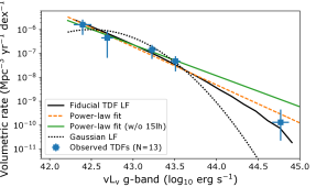
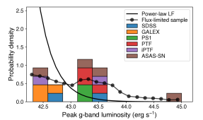
Here denotes the product of the effective survey duration and survey area, and is the volume (per unit solid angle) corresponding to the maximum redshift. As explained in Sec. 2, the product of the effective survey duration and survey area follows from the detected number of TDF candidates, while the maximum volume follows from the survey flux limit and the peak luminosity of the transient. In Figs. 1 and 2 we show binned by the peak -band luminosity and galaxy mass, respectively. Since the PTF search for TDFs (Arcavi et al., 2014) used a luminosity selection (see Sec. 2.1.4), we exclude these events when we compute the rate as a function of . We also have to exclude iPTF-15af since the photometric data of this flare have not been published yet. We are thus left with sources. For TDFs with a measurement of the host galaxy velocity dispersion, the black hole mass is estimated from the – relation (Ferrarese & Merritt, 2000; Gebhardt et al., 2000). We adopt the relation of Gültekin et al. (2009), obtained using both early-type and late-type galaxies. For the TDF host galaxies that have measured velocity dispersions, we compute the maximum volume using the lower value of from the flux limit for the detection of the flare and the host galaxy flux limit for measuring the velocity dispersion—the former is the limiting factor for most sources (see the last column of Table 1 and Table 2). The uncertainty on each bin of is estimated from (Schmidt, 1968). This yields a typical uncertainty of 0.3 dex for each bin, which is comparable to the Poisson uncertainty. For bins that contain only one source, we compute the uncertainty on the volumetric rate using the 1 confidence interval for Poisson statistics, [0.17, 3.41]. The sum of for all 13 TDF candidates that we use for the LF yields a rate of . The volumetric rate as a function of (Fig. 1) shows a steep decrease that can be parameterized as
| (4) |
For , a least-squares fit yields and . If we exclude the luminous TDF candidate ASASSN-15lh, we find a more shallow slope with a larger uncertainty: and . When excluding ASASSN-15lh, a Gaussian function
| (5) |
with , , and , also provides a reasonable description of the LF (Fig. 1).
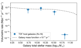
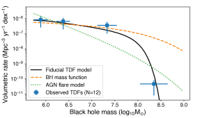
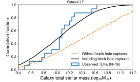
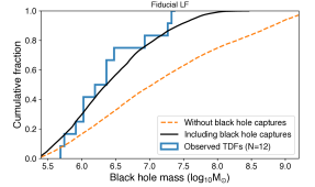
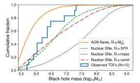
To convert our measurement of the volumetric TDF rate to a rate per galaxy, we compute the volumetric rate as a function of total stellar mass and divide by the stellar mass function of Baldry et al. (2012). For a stellar mass in the range a constant rate of galaxy-1 yr-1 is consistent with our observations (Fig. 2). The rate as a function of black hole mass (Fig. 3) is also observed to be roughly constant for . However, the high luminosity of the TDF candidate ASASSN-15lh yields a very large and thus implies a rapid decrease of the volumetric rate for . The decrease of the rate toward the highest-mass bin is at least 3 orders of magnitude. Arguably the only conceivable mechanism that can yield such an extreme turnover is the suppression of the flare rate by the black hole horizon. We can thus conclude that if ASASSN-15lh is a member of the TDE family, the population of observed TDFs as a whole is consistent with the predicted suppression of the rate due to the direct capture of stars by the black hole. However, if ASASSN-15lh is not due to a TDE, the mass function of the remaining TDFs in our sample is not a useful tool to measure rate suppression. Instead, we need to compare the observed mass distribution to the expected distribution in a flux-limited sample. This requires a forward-modeling approach, which is explained in the next section.
4. Forward Modeling
In the previous section we used the method to reconstruct the TDF LF and mass function. In this section, we start with a model for the flare luminosity function and event rate and try to reproduce the observed distribution of luminosity and host galaxy mass. This forward-modeling approach has two advantages over a reconstruction. First of all, we can include additional selection criteria beyond the survey flux limit (e.g., the contrast between the flux of the host and flare). Second, we can assign a significance to the apparent lack of events from high-mass black holes. Our forward-modeling method consists of four steps: (i) draw flares with a peak luminosity from a model LF; (ii) insert these flares into a flux-limited galaxy sample; (iii) assign each flare a weight based on the event rate in its host galaxy; (iv) sum these weights for the simulated flares that pass the requirement for detection in each survey. In the following four subsections we provide the details of these steps.
4.1. Model Luminosity Functions
Ideally, a model for TDFs or TDF impostors would yield a prediction for the LF of these events that can be tested using the observed luminosity distribution (Fig. 4). However, these models are not yet mature enough to predict an LF from first principles. We therefore use a more empirical approach and only consider LFs that are known to reproduce the observed luminosity distribution. We will consider two different LFs: one for SNe and one for AGN flares and TDFs. The observed LF from the 1/ method (Fig. 1) provides a good starting point for our empirical LF models. Indeed, if we draw TDFs from a power-law LF with (see Eq. 4) and apply the survey selection criteria (see Sec. 4.4) we reproduce the observed distribution of , see Fig. 4. We therefore use this power law as the model LF of nuclear SNe. A simple power law is unlikely to provide a correct description of the LF of transients that are due to massive black holes, i.e., TDFs or AGN flares. Due to the abundance of low-mass galaxies, a power-law LF will yield too many transients with super-Eddington luminosities. Motivated by the observation that the observed distribution of the Eddington ratio peaks near unity (Fig. 7), we define the LF for AGN flares and TDFs as follows. We draw from the same power law that is used to model SNe, but we only accept flares with an Eddington ratio in the range . Here , with erg s-1. To assign a bolometric luminosity () to each simulated flare, we compute the blackbody luminosity by drawing a blackbody temperature from a lognormal distribution centered on K with a standard deviation of 0.15 dex (which provides a good description of the observed blackbody temperatures of the TDF candidates in our sample). The resulting LF for TDFs and AGN flares using this approach is shown in Fig. 1. The next step is to insert the simulated flares into a host galaxy sample.
4.2. Synthetic Galaxy Sample
While large galaxy surveys like SDSS provide a good census of galaxy properties at , many TDFs are found at higher redshift, where galaxy properties are more difficult to observe directly. We therefore need to construct a synthetic galaxy sample.
We use the galaxy LF measured by Cool et al. (2012) to find the number of galaxies in bins of redshift and absolute magnitude, for blue and red galaxies separately. We populate each bin using the properties of real galaxies from the NYU-Valued-Added Galaxy Catalog (NYU-VAGC; Blanton et al., 2005), again for red and blue galaxies separately. In each bin, we compute the apparent magnitude using the median k-correction of the galaxies in that bin. We keep only bins with an apparent magnitude .
Because we use a redshift-dependent LF for blue and red galaxies (Cool et al., 2012), our synthetic flux-limited galaxy sample contains most effects of galaxy evolution (e.g., the increase of the quiescent-galaxy density to lower redshift). Our approach also accounts for the fact that blue galaxies are easier to detect at higher redshift (due to the k-correction). And finally, because we use real galaxies to populate each absolute magnitude bin, correlations of galaxy properties (e.g., mass or size) with luminosity are part of our sample. We confirmed that the median redshift of our synthetic galaxy sample, , is consistent with the median photometric redshift of real galaxies (also selected with ) in the co-add of SDSS Stripe 82 (Reis et al., 2012; Annis et al., 2014).
The total stellar mass of each galaxy in NYU-VAGC is estimated from the 2MASS and SDSS broadband photometry using the correct software \citep{blanton07}. To estimate the starformation rate (SFR), we use the specific SFR within the SDSS spectroscopic fiber as measured by the MPA-JHU group \citep{Kauffmann03b,Brinchmann04}. To estimate the bulge mass, we use the bulge-to-total ratio ($B/T$) measured in $r$ band by \citet{Lacner12. These measurements are not available for all NYU-VAGC galaxies, so we assigned each galaxy in our synthetic sample a using the nearest match in the 3D vector space spanned by , , and .
The last quantity we wish to assign to our synthetic galaxy sample is the velocity dispersion. Unfortunately, the resolution of the SDSS spectrograph limits reliable measurements to km s-1, which is larger than the typical velocity dispersion of TDF host galaxies (Wevers et al., 2017). Following the approach of Bezanson et al. (2011), we use the virial theorem to estimate the velocity dispersion of each galaxy,
| (6) |
Here is the effective radius, is a scale factor that accounts for the mean difference between the dynamical mass and the stellar mass estimated from the photometry (Taylor et al., 2010), and is a virial constant (Bertin et al., 2002) that depends on the Sersic index (),
| (7) |
Using the stellar mass, effective radii, and Sersic indices reported in the NYU-VAGC (Blanton et al., 2005), we find that is required to match the observed velocity dispersion to the estimate from Eq. 6. This calibration is consistent with the value of reported by Bezanson et al. (2012). For km s-1, the scatter between the observed value of the velocity dispersion and the value from Eq. 6 is 0.08 dex. The bulge mass and velocity dispersion can be used to estimate the mass of the black hole at the galaxy’s center. We use the Gültekin et al. (2009) – relation for their sample of “all” galaxies (i.e., both early-types and late-types):
| (8) |
To estimate the black hole mass from the bulge mass, we adopt the Gültekin et al. (2009) – relation, and we use the NYU-VAGC galaxies to measure the small correction to the power-law index due to the luminosity dependence of the mass-to-light ratio, which yields
| (9) |
We apply Gaussian noise with a standard deviation of 0.4 dex (Gültekin et al., 2009) when assigning the black hole mass based on the host galaxy properties. We find that the two methods to estimate the black hole mass agree reasonably well; the difference between using the velocity dispersion and the galaxy bulge mass roughly scales as dex, with the mass from the – relation. Since reliable measurements are not available for most of the TDF candidates in our sample, we will use the black hole mass estimate from the - relation as the default value in our analysis. We simulated galaxies. This sample is available online (see Table 5).
| SNe | AGN flares | |
| SNe | – | |
| SNe | – | |
| – | AGN flares | |
| Eq. 10 | – | TDFs |
Note. — The cells of this matrix show which combinations of event rate (rows) and luminosity function (columns) are considered as a description for AGN flares, nuclear SNe, or TDFs. The two luminosity functions have the same power-law index, but the function used for TDFs and AGN flares is capped based on the ratio of the blackbody luminosity to the Eddington luminosity ().
4.3. Model Event Rates
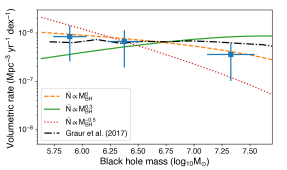
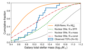
We consider four possible models for the scaling of the event rate with galaxy properties. First of all, the simplest assumption is a galaxy-independent rate. Next, we consider an event rate proportional to the SFR. This scaling could be expected if current optical TDF candidates are due to a new type of stellar explosion in galactic nuclei (Saxton et al., 2016). To model flares caused by AGN disk instabilities, we consider an event rate that is inversely proportional to central black hole mass, (i.e., the wait time between outbursts is proportional to the black hole mass; see Sec. 5.2). Finally, to estimate the rate of flares due to TDEs, we use the following equation:
| (10) |
The power-law index parameterizes how the disruption rate changes due to the dynamics of the host galaxy; predictions for this index range from (Brockamp et al., 2011), to (Wang & Merritt, 2004; Kochanek, 2016), and (Stone & Metzger, 2016). All of these predictions are broadly consistent with the observed mass function derived from the method, but steeper power laws can be ruled out (see Fig. 3, bottom panel). For our fiducial TDF model, we adopt , the relation predicted for an isothermal sphere (cf. Wang & Merritt, 2004, Eq. 29). Our parameterization of the turnover in the TDF rate approximates the curve of Kesden (2012, , Figure 4) for a solar-type star disrupted by a black hole with a spin of . Finally, in Fig. 3 we also compare our estimate of the TDF rate as a function of mass with the result of Graur et al. (2017), who conclude that this rate is proportional to , with the galaxy surface mass density. For this comparison, we computed for the galaxies in our mock sample and binned the result as a function of black hole mass.
4.4. Mock TDF Samples
The last step of our forward-modeling analysis is applying the selection criteria of the surveys. Summing the event rate of simulated flares that pass the selection criteria yields the final output: a mock version of our flux-limited TDF sample (Table 1). Besides the obvious requirement that the peak flux of the simulated flare is larger than the effective survey flux limit, we also require that the magnitude difference between the simulated flare and the host galaxy () is less than 3 mag (which corresponds to the lowest host-flare contrast in our sample of candidate TDFs). For simulated flares observed by the PTF survey we also apply their luminosity cut (;see Sec. 2.1.4). Similar to our method for normalizing the effective area in the analysis, we require that the ratio of the simulated flares detected by each survey is equal to the ratio of detected TDF candidates for these surveys (see Table 3). We now compare the observed distribution111In Figs. 5–7 we show the observed distributions without ASASSN-15lh. of galaxy mass or black hole mass of the host galaxies of our TDF candidates with the distribution obtained for a simulated sample with and without a correction for captures (Fig. 5). We find that the simulation without a correction for captures overpredicts the number of flares from high-mass black holes. Using a Kolmogorov–Smirnov (KS) test, the hypothesis that the host galaxy stellar mass of the mock sample without captures and the host galaxy mass of observed candidate TDFs are drawn from the same distribution can be rejected with . If we apply the same test to the distribution of black hole mass, we again reject the null hypothesis, but with slightly lower significance (, due to the smaller sample size). Repeating this exercise using a Gaussian LF (Eq. 5) instead of an power-law LF (Eq. 4) does not change the significance of the detection of rate suppression by black hole event horizons. Since we use the number of detected TDF candidates in each survey to normalize the contribution of the different surveys to the final sample of mock TDFs, the small number of flares in each survey introduces a statistical uncertainty that is not captured in a single KS test. To estimate this uncertainty, we compute multiple mock samples, drawing the number of candidate TDFs in each surveys from a Poisson distribution centered on . For each of these samples, we compute the -value for rejecting the null hypothesis. The distribution of the resulting -values follows a lognormal distribution with a standard deviation of only 0.2 dex. We can thus conclude that Poisson fluctuation in the number of detected TDF candidates will not lead to a false detection of horizon suppression (a 9 fluctuation of is required to reach ). The simulated distributions of galaxy mass and black hole mass for the other three scenarios that we consider (see Table 4) are shown in Fig. 6.
5. Discussion
5.1. TDFs Are Not Due to Stellar Explosions
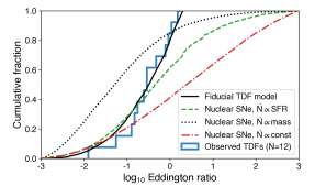
We find that our fiducial TDF model correctly reproduces the distribution of host galaxy total stellar mass, host galaxy black holes mass, and Eddington ratio (see Fig. 5 and Fig. 7). From Fig. 6, we conclude that if the observed TDFs are due to a hypothetical new class of nuclear SNe, the rate of these events needs to be independent of host galaxy mass or SFR. This requirement could be considered unlikely, because the rate of most types of known SNe either scales with the host galaxy surface brightness or is limited to a particular subset of galaxies (e.g., Fruchter et al., 2006). The strongest evidence against the possibility that observed optical TDF candidates are a new class of SNe is the observed distribution of the Eddington ratio. The Eddington limit for photons does not apply to stellar explosions, but for each simulated SN we can still compute the Eddington ratio based on the central black hole mass of its host galaxy. If the flare rate is independent of galaxy properties and not constrained by the Eddington limit, more than half of the observed optical TDF candidates should have super-Eddington luminosities (Fig. 7). The luminosity of candidate TDFs, however, is observed to be capped near the Eddington luminosity. The probability that a flux-limited SN sample would produce this skewed distribution of is small (KS test yields ). We find the same result if we use a Gaussian distribution (Eq. 5) to draw the luminosity of the simulated SNe.
5.2. TDFs Are Unlikely Due to AGN
An instability in an AGN accretion disk could lead to a rapid increase of the accretion rate and may therefore mimic a TDF. This scenario has several problems, such as the observed evolution of the broad emission lines of known candidate TDFs, which get more narrow with time, while AGN show the opposite behavior (Ruan et al., 2016; Holoien et al., 2016b). But such problems are not insurmountable because the parameter space of AGN disk instabilities has not been fully explored yet. Our work provides a test of the AGN flare scenario with minimal requirements. The only model prediction that is needed is the scaling of the flare rate with black hole mass. The wait time between AGN outbursts depends on the black hole mass and the accretion rate. If the accretion rate normalized to the Eddington limit is constant over the mass range relevant for our TDF sample, the wait time between outbursts from active black holes is predicted to scale as , with (Mineshige & Shields, 1990; Siemiginowska & Elvis, 1997). The increased wait time and longer flare duration reduce the rate of detected AGN flares from massive black holes, potentially explaining the lack of TDF candidates at high mass. However, we find that a scenario with predicts too many flares at the low-mass end (Figs. 3 & 6). If instead the rate of AGN flares is independent of mass (), a flux-limited sample of AGN flares should contain many more events from black holes with a mass (Fig. 5). We can thus conclude that most AGN flare scenarios are inconsistent with the observed mass distribution of TDF host galaxies. One caveat is that most AGN outburst models assume that the disk remains radiatively efficient between outbursts. It would be interesting to compare predictions for the rate of sub-Eddington AGN (e.g., LINERs) going into outburst. Besides instabilities, stellar collisions near the tidal radius could also produce TDF impostors (Metzger & Stone, 2017). These collisions happen between stars that accrete onto the central black hole via Roche lobe overflow, and therefore they are only possible when the Roche radius lies outside the innermost stable circular orbit. The rate of these collisions will therefore diminish above a mass scale similar to the Hills mass of TDEs and could thus explain the observed turnover in the TDF mass function (Fig. 3). However, multiple grazing collisions of the same stars are required to get a sufficiently high rate of these events, and around larger supermassive black holes, stars are often destroyed by their relativistic collision velocities. As a result, rate suppression in the stellar collision model likely occurs at an order of magnitude lower black hole mass (; Metzger & Stone 2017), which is inconsistent with our observations.
5.3. Detection of Horizon Suppression
The only scenario that can explain both the distribution of the Eddington ratio and the distribution of black hole mass requires a roughly constant rate up to a black hole mass of , followed by a rapid decrease toward higher mass. This, indeed, is a fundamental prediction of the TDE paradigm. The location of the turnover scales with black hole spin and the density of the disrupted star. Assuming that for black holes with a mass of most of the disrupted stars are similar to the Sun (e.g., Kochanek, 2016), our mass function appears to imply a relatively high mean spin of black holes in this mass regime—perhaps similar to the spins inferred using observations of the iron fluorescence line in nearby AGN (Risaliti et al., 2013; Reynolds, 2014). The detection of more events similar to ASASSN-15lh will be key to making a more robust inference of black hole spin from the TDF black hole mass function. Our measurement of the turnover in the black hole mass function relies on the - relation to estimate this mass, and therefore it is subject to the systematic uncertainty associated with the calibration of this relation. However, the turnover is also clearly detected in the distribution of total stellar mass (Figs. 2 and 5): for the event rate to be independent of galaxy mass, 50% of the TDFs in our compilation should have a host galaxy mass . Instead, only 3 out of 17 (including ASASSN-15lh) are found above this host galaxy mass limit. The stellar mass of TDF host galaxies and the synthetic host galaxy sample are calculated using the same method; hence the systematic uncertainty of this result is negligible. At the low end of the host galaxy mass spectrum, we find no significant decrease of the number of flares compared to what is expected in a flux-limited survey. This could be considered surprising, since circularization and accretion of the stellar debris for disruptions around low-mass black holes are predicted to be less efficient (Guillochon & Ramirez-Ruiz, 2015). Our observations thus support a constant black hole occupation fraction for . Post-starburst galaxies (characterized as quiescent galaxies with strong Balmer absorption lines; Dressler & Gunn 1983; Zabludoff et al. 1996) are overrepresented among TDF hosts (Arcavi et al., 2014; French et al., 2016, 2017; Law-Smith et al., 2017; Graur et al., 2017), which could be explained by a short relaxation time caused by a high central density in these galaxies (Stone & van Velzen, 2016; Graur et al., 2017). An overrepresentation of post-starburst galaxies is unlikely to significantly influence the distribution of total stellar mass of the mock TDF sample because the relative mass increase in the recent star-formation episode of these galaxies is modest, 10–50%, (Kaviraj et al. 2007; D. French et al., in prep). Since we use the total stellar light to estimate the galaxy mass (including the old stars as measured by the near-IR flux), a post-starburst phase of TDF host galaxies will not lead to a significant change of the total stellar mass in the mock sample. Our results are consistent with the recent work by Lu, Kumar, & Narayan (2017), who used the lack of TDF candidates from high-mass black holes to rule out the hypothesis that supermassive black holes have a surface (at some small fraction above the Schwarzschild radius).
5.4. The Luminosity Function of TDFs
Our work is the first to measure the shape of the LF of optical/UV-selected TDFs. We find that a steep power law provides a good description, (Eq. 4). About one-third of the candidate TDFs in our sample were discovered after the peak in the light curve and this introduces a systematic uncertainty to the LF. If the true peak luminosity of all of the sources discovered after maximum light is a factor of 2 higher than the observed maximum luminosity, the power-law index of the LF decreases by about 10%. While the TDF LF is steep, both the observed rate as a function of black hole mass (Fig. 3) and the peak luminosity of the flare (Hung et al., 2017) appear to be independent of black hole mass (for ). Here we speculated that this might imply that the wide range in TDF peak luminosity is determined by the mass of the star that got disrupted. For a main-sequence mass–radius relation, the peak of the fallback rate of stellar debris is expected to scale as (e.g., Guillochon & Ramirez-Ruiz, 2013). If the peak luminosity is proportional to this fallback rate, a Kroupa et al. (1993) initial mass function ( for ) would yield a steep decrease of the event rate with peak luminosity. Since the Hills mass is proportional to the mass of the disrupted star, this scenario implies that low-luminosity TDFs, such as iPTF-16fnl, only occur in relatively low-mass host galaxies, while high-luminosity TDFs can occur across a wider host galaxy mass range. The steep flare LF also explains why our measurement of the average per-galaxy rate (; Fig. 2) is higher than the rate based on SDSS data (van Velzen & Farrar, 2014) or ASAS-SN data (Holoien et al., 2016b). In the SDSS analysis, the per-galaxy rate follows from , with the search efficiency times the number of galaxies that were surveyed. Because the average TDF rate was computed using the mean of this efficiency, the brightest flare contributes more to the per-galaxy rate (the difference in between SDSS-TDE1 and SDSS-TDE2 is factor of 4; see van Velzen & Farrar 2014, Table 1). The efficiency-weighted mean luminosity of the two SDSS flares is . The rate from our LF (Fig. 1) at this relatively high luminosity is , which is consistent with the volumetric rate reported from the SDSS search. Our measurement of the per-galaxy flare rate (Fig. 2) is consistent with the theoretical predictions of the disruption rate by Stone & Metzger (2016), who find galaxy-1 yr-1. As forecasted by Kochanek (2016), it appears that the tension between earlier measurements of the TDF rate and the theoretically expected rate could simply be due to the relatively high luminosity of the TDFs in these surveys. When accounting for our observation that faint TDFs occur more frequently, the discrepancy between the observed and predicted rate disappears. The total rate of TDFs depends on the low-luminosity turnover of the LF, which is not constrained by our current sample of flares. However, if the bolometric luminosity of TDFs is capped near the Eddington limit, the LF should start to flatten just below the luminosity of the faintest flares in our sample (for a typical bolometric correction of , a -band luminosity of exceeds the Eddington limit for black holes with ). For an Eddington-limited emission mechanism, the peak of the luminosity distribution in a flux-limited sample shifts to higher black hole mass (Kochanek, 2016). This could explain why the turnover of the LF has not been detected yet.
6. Conclusions
Our main conclusions are as follows:
- •
-
•
For galaxies with a stellar mass of , the observed per-galaxy rate is yr-1 (Fig. 2).
-
•
We measured the black hole mass function of TDF host galaxies (Fig. 3), finding an approximately constant volumetric rate for .
-
•
The sharp decrease of the volumetric rate above , as implied by the high-luminosity TDF candidate ASASSN-15lh, is consistent with the suppression of the TDF rate due to the capture of stars before they are disrupted.
-
•
Rate suppression due to black hole event horizons can also be detected while remaining agnostic about the origin of ASASSN-15lh. Using forward modeling to reproduce our flux-limited TDF sample, we conclude that rate suppression at high black hole mass plus an Eddington-limited emission mechanism are both required to explained the observed distribution of galaxy mass and Eddington ratio (Figs. 5–7).
References
- Abazajian et al. (2009) Abazajian, K. N., Adelman-McCarthy, J. K., Agüeros, M. A., et al. 2009, ApJS, 182, 543
- Alexander et al. (2017) Alexander, K. D., Wieringa, M. H., Berger, E., Saxton, R. D., & Komossa, S. 2017, ApJ, 837, 153
- Annis et al. (2014) Annis, J., Soares-Santos, M., Strauss, M. A., et al. 2014, ApJ, 794, 120
- Arcavi et al. (2014) Arcavi, I., Gal-Yam, A., Sullivan, M., et al. 2014, ApJ, 793, 38
- Astropy Collaboration et al. (2013) Astropy Collaboration, Robitaille, T. P., Tollerud, E. J., et al. 2013, A&A, 558, A33
- Auchettl et al. (2017a) Auchettl, K., Guillochon, J., & Ramirez-Ruiz, E. 2017a, ApJ, 838, 149
- Auchettl et al. (2017b) Auchettl, K., Ramirez-Ruiz, E., & Guillochon, J. 2017b, ArXiv e-prints, arXiv:1703.06141
- Bade et al. (1996) Bade, N., Komossa, S., & Dahlem, M. 1996, A&A, 309, L35
- Baldry et al. (2012) Baldry, I. K., Driver, S. P., Loveday, J., et al. 2012, MNRAS, 421, 621
- Bertin et al. (2002) Bertin, G., Ciotti, L., & Del Principe, M. 2002, A&A, 386, 149
- Bezanson et al. (2012) Bezanson, R., van Dokkum, P., & Franx, M. 2012, ApJ, 760, 62
- Bezanson et al. (2011) Bezanson, R., van Dokkum, P. G., Franx, M., et al. 2011, ApJ, 737, L31
- Bielby et al. (2012) Bielby, R., Hudelot, P., McCracken, H. J., et al. 2012, A&A, 545, A23
- Blagorodnova et al. (2017) Blagorodnova, N., Gezari, S., Hung, T., et al. 2017, ApJ, 844, 46
- Blanchard et al. (2017) Blanchard, P. K., Nicholl, M., Berger, E., et al. 2017, ApJ, 843, 106
- Blanton & Roweis (2007) Blanton, M. R., & Roweis, S. 2007, AJ, 133, 734
- Blanton et al. (2001) Blanton, M. R., Dalcanton, J., Eisenstein, D., et al. 2001, AJ, 121, 2358
- Blanton et al. (2005) Blanton, M. R., Schlegel, D. J., Strauss, M. A., et al. 2005, AJ, 129, 2562
- Bloom et al. (2011) Bloom, J. S., Giannios, D., Metzger, B. D., et al. 2011, Science, 333, 203
- Brinchmann et al. (2004) Brinchmann, J., Charlot, S., White, S. D. M., et al. 2004, MNRAS, 351, 1151
- Brockamp et al. (2011) Brockamp, M., Baumgardt, H., & Kroupa, P. 2011, MNRAS, 418, 1308
- Brown et al. (2017) Brown, J. S., Holoien, T. W.-S., Auchettl, K., et al. 2017, MNRAS, 466, 4904
- Brown et al. (2016) Brown, J. S., Shappee, B. J., W.-S Holoien, T., et al. 2016, MNRAS, 462, 3993
- Brown et al. (2018) Brown, J. S., Kochanek, C. S., Holoien, T. W.-S., et al. 2018, MNRAS, 473, 1130
- Cenko et al. (2012) Cenko, S. B., Bloom, J. S., Kulkarni, S. R., et al. 2012, MNRAS, 420, 2684
- Chambers (2007) Chambers, K. C. 2007, in Bulletin of the AAS, Vol. 38, 995
- Chambers et al. (2016) Chambers, K. C., Magnier, E. A., Metcalfe, N., et al. 2016, ArXiv e-prints, arXiv:1612.05560
- Chornock et al. (2014) Chornock, R., Berger, E., Gezari, S., et al. 2014, ApJ, 780, 44
- Cool et al. (2012) Cool, R. J., Eisenstein, D. J., Kochanek, C. S., et al. 2012, ApJ, 748, 10
- Czerny et al. (2009) Czerny, B., Siemiginowska, A., Janiuk, A., Nikiel-Wroczyński, B., & Stawarz, Ł. 2009, ApJ, 698, 840
- Dai et al. (2015) Dai, L., McKinney, J. C., & Miller, M. C. 2015, ApJ, 812, L39
- Dong et al. (2016) Dong, S., Shappee, B. J., Prieto, J. L., et al. 2016, Science, 351, 257
- Drake et al. (2011) Drake, A. J., Djorgovski, S. G., Mahabal, A., et al. 2011, ApJ, 735, 106
- Dressler & Gunn (1983) Dressler, A., & Gunn, J. E. 1983, ApJ, 270, 7
- Ferrarese & Merritt (2000) Ferrarese, L., & Merritt, D. 2000, ApJ, 539, L9
- Flewelling et al. (2016) Flewelling, H. A., Magnier, E. A., Chambers, K. C., et al. 2016, ArXiv e-prints, arXiv:1612.05243
- French et al. (2016) French, K. D., Arcavi, I., & Zabludoff, A. 2016, ApJ, 818, L21
- French et al. (2017) —. 2017, ApJ, 835, 176
- Frieman et al. (2008) Frieman, J. A., Bassett, B., Becker, A., et al. 2008, AJ, 135, 338
- Fruchter et al. (2006) Fruchter, A. S., Levan, A. J., Strolger, L., et al. 2006, Nature, 441, 463
- Gebhardt et al. (2000) Gebhardt, K., Bender, R., Bower, G., et al. 2000, ApJ, 539, L13
- Gezari et al. (2015) Gezari, S., Chornock, R., Lawrence, A., et al. 2015, ApJ, 815, L5
- Gezari et al. (2006) Gezari, S., Martin, D. C., Milliard, B., et al. 2006, ApJ, 653, L25
- Gezari et al. (2008) Gezari, S., Basa, S., Martin, D. C., et al. 2008, ApJ, 676, 944
- Gezari et al. (2009) Gezari, S., Heckman, T., Cenko, S. B., et al. 2009, ApJ, 698, 1367
- Gezari et al. (2012) Gezari, S., Chornock, R., Rest, A., et al. 2012, Nature, 485, 217
- Gezari et al. (2017) Gezari, S., Hung, T., Cenko, S. B., et al. 2017, ApJ, 835, 144
- Godoy-Rivera et al. (2017) Godoy-Rivera, D., Stanek, K. Z., Kochanek, C. S., et al. 2017, MNRAS, 466, 1428
- Graham et al. (2017) Graham, M. J., Djorgovski, S. G., Drake, A. J., et al. 2017, MNRAS, 470, 4112
- Graur et al. (2017) Graur, O., French, K. D., Zahid, H. J., et al. 2017, ArXiv e-prints, arXiv:1707.02986
- Grogin et al. (2011) Grogin, N. A., Kocevski, D. D., Faber, S. M., et al. 2011, ApJS, 197, 35
- Guillochon et al. (2014) Guillochon, J., Manukian, H., & Ramirez-Ruiz, E. 2014, ApJ, 783, 23
- Guillochon & Ramirez-Ruiz (2013) Guillochon, J., & Ramirez-Ruiz, E. 2013, ApJ, 767, 25
- Guillochon & Ramirez-Ruiz (2015) —. 2015, ApJ, 809, 166
- Gültekin et al. (2009) Gültekin, K., Richstone, D. O., Gebhardt, K., et al. 2009, ApJ, 698, 198
- Hambly et al. (2008) Hambly, N. C., Collins, R. S., Cross, N. J. G., et al. 2008, MNRAS, 384, 637
- Hameury et al. (2009) Hameury, J.-M., Viallet, M., & Lasota, J.-P. 2009, A&A, 496, 413
- Hatziminaoglou et al. (2001) Hatziminaoglou, E., Siemiginowska, A., & Elvis, M. 2001, ApJ, 547, 90
- Heckman (1980) Heckman, T. M. 1980, A&A, 87, 152
- Hills (1975) Hills, J. G. 1975, Nature, 254, 295
- Hogg et al. (2002) Hogg, D. W., Baldry, I. K., Blanton, M. R., & Eisenstein, D. J. 2002, ArXiv astro-ph/0210394, astro-ph/0210394
- Holoien et al. (2014) Holoien, T. W.-S., Prieto, J. L., Bersier, D., et al. 2014, MNRAS, 445, 3263
- Holoien et al. (2016a) Holoien, T. W.-S., Kochanek, C. S., Prieto, J. L., et al. 2016a, MNRAS, 463, 3813
- Holoien et al. (2016b) —. 2016b, MNRAS, 455, 2918
- Hung et al. (2017) Hung, T., Gezari, S., Blagorodnova, N., et al. 2017, ApJ, 842, 29
- Janiuk et al. (2002) Janiuk, A., Czerny, B., & Siemiginowska, A. 2002, ApJ, 576, 908
- Jarrett et al. (2000) Jarrett, T. H., Chester, T., Cutri, R., et al. 2000, AJ, 119, 2498
- Jiang et al. (2016) Jiang, N., Dou, L., Wang, T., et al. 2016, ApJ, 828, L14
- Kauffmann et al. (2003) Kauffmann, G., Heckman, T. M., White, S. D. M., et al. 2003, MNRAS, 341, 33
- Kaviraj et al. (2007) Kaviraj, S., Kirkby, L. A., Silk, J., & Sarzi, M. 2007, MNRAS, 382, 960
- Kesden (2012) Kesden, M. 2012, Phys. Rev. D, 85, 024037
- Kochanek (2016) Kochanek, C. S. 2016, MNRAS, 461, 371
- Koekemoer et al. (2011) Koekemoer, A. M., Faber, S. M., Ferguson, H. C., et al. 2011, ApJS, 197, 36
- Komossa (2015) Komossa, S. 2015, Journal of High Energy Astrophysics, 7, 148
- Komossa & Bade (1999) Komossa, S., & Bade, N. 1999, A&A, 343, 775
- Komossa et al. (2008) Komossa, S., Zhou, H., Wang, T., et al. 2008, ApJ, 678, L13
- Krolik et al. (2016) Krolik, J., Piran, T., Svirski, G., & Cheng, R. M. 2016, ApJ, 827, 127
- Kroupa et al. (1993) Kroupa, P., Tout, C. A., & Gilmore, G. 1993, MNRAS, 262, 545
- Krühler et al. (2017) Krühler, T., Fraser, M., Leloudas, G., et al. 2017, ArXiv e-prints, arXiv:1710.01045
- Lackner & Gunn (2012) Lackner, C. N., & Gunn, J. E. 2012, MNRAS, 421, 2277
- LaMassa et al. (2015) LaMassa, S. M., Cales, S., Moran, E. C., et al. 2015, ApJ, 800, 144
- Lang et al. (2014) Lang, D., Hogg, D. W., & Schlegel, D. J. 2014, ArXiv e-prints, arXiv:1410.7397
- Lasota (2001) Lasota, J.-P. 2001, New A Rev., 45, 449
- Law et al. (2009) Law, N. M., Kulkarni, S. R., Dekany, R. G., et al. 2009, PASP, 121, 1395
- Law-Smith et al. (2017) Law-Smith, J., Ramirez-Ruiz, E., Ellison, S. L., & Foley, R. J. 2017, ApJ, 850, 22
- Lawrence et al. (2007) Lawrence, A., Warren, S. J., Almaini, O., et al. 2007, MNRAS, 379, 1599
- Leloudas et al. (2016) Leloudas, G., Fraser, M., Stone, N. C., et al. 2016, Nature Astronomy, 1, 0002
- Levan et al. (2011) Levan, A. J., Tanvir, N. R., Cenko, S. B., et al. 2011, Science, 333, 199
- Lodato & Rossi (2011) Lodato, G., & Rossi, E. M. 2011, MNRAS, 410, 359
- Lu et al. (2017) Lu, W., Kumar, P., & Narayan, R. 2017, MNRAS, 468, 910
- MacLeod et al. (2012) MacLeod, C. L., Ivezić, Ž., Sesar, B., et al. 2012, ApJ, 753, 106
- MacLeod et al. (2016) MacLeod, C. L., Ross, N. P., Lawrence, A., et al. 2016, MNRAS, 457, 389
- MacLeod et al. (2014) MacLeod, M., Goldstein, J., Ramirez-Ruiz, E., Guillochon, J., & Samsing, J. 2014, ApJ, 794, 9
- Mainzer et al. (2014) Mainzer, A., Bauer, J., Cutri, R. M., et al. 2014, ApJ, 792, 30
- Maksym et al. (2013) Maksym, W. P., Ulmer, M. P., Eracleous, M. C., Guennou, L., & Ho, L. C. 2013, MNRAS, 435, 1904
- Margutti et al. (2017) Margutti, R., Metzger, B. D., Chornock, R., et al. 2017, ApJ, 836, 25
- Martin et al. (2005) Martin, D. C., Fanson, J., Schiminovich, D., et al. 2005, ApJ, 619, L1
- Merloni et al. (2015) Merloni, A., Dwelly, T., Salvato, M., et al. 2015, MNRAS, 452, 69
- Metzger & Stone (2016) Metzger, B. D., & Stone, N. C. 2016, MNRAS, 461, 948
- Metzger & Stone (2017) —. 2017, ApJ, 844, 75
- Meyer & Meyer-Hofmeister (1981) Meyer, F., & Meyer-Hofmeister, E. 1981, A&A, 104, L10
- Mineshige & Shields (1990) Mineshige, S., & Shields, G. A. 1990, ApJ, 351, 47
- Oke (1974) Oke, J. B. 1974, ApJS, 27, 21
- Pasham et al. (2017) Pasham, D. R., Cenko, S. B., Sadowski, A., et al. 2017, ApJ, 837, L30
- Piran et al. (2015) Piran, T., Svirski, G., Krolik, J., Cheng, R. M., & Shiokawa, H. 2015, ApJ, 806, 164
- Rees (1988) Rees, M. J. 1988, Nature, 333, 523
- Reis et al. (2012) Reis, R. R. R., Soares-Santos, M., Annis, J., et al. 2012, ApJ, 747, 59
- Reynolds (2014) Reynolds, C. S. 2014, Space Sci. Rev., 183, 277
- Risaliti et al. (2013) Risaliti, G., Harrison, F. A., Madsen, K. K., et al. 2013, Nature, 494, 449
- Ruan et al. (2016) Ruan, J. J., Anderson, S. F., Cales, S. L., et al. 2016, ApJ, 826, 188
- Saxton et al. (2016) Saxton, C. J., Perets, H. B., & Baskin, A. 2016, ArXiv e-prints, arXiv:1612.08093
- Saxton et al. (2017) Saxton, R. D., Read, A. M., Komossa, S., et al. 2017, A&A, 598, A29
- Schlafly & Finkbeiner (2011) Schlafly, E. F., & Finkbeiner, D. P. 2011, ApJ, 737, 103
- Schmidt (1968) Schmidt, M. 1968, ApJ, 151, 393
- Shankar et al. (2004) Shankar, F., Salucci, P., Granato, G. L., De Zotti, G., & Danese, L. 2004, MNRAS, 354, 1020
- Shappee et al. (2014) Shappee, B. J., Prieto, J. L., Grupe, D., et al. 2014, ApJ, 788, 48
- Siemiginowska & Elvis (1997) Siemiginowska, A., & Elvis, M. 1997, ApJ, 482, L9
- Skrutskie et al. (1997) Skrutskie, M. F., Schneider, S. E., Stiening, R., et al. 1997, in Astrophysics and Space Science Library, Vol. 210, The Impact of Large Scale Near-IR Sky Surveys, ed. F. Garzon, N. Epchtein, A. Omont, B. Burton, & P. Persi, 25
- Smak (1983) Smak, J. 1983, ApJ, 272, 234
- Stefanon et al. (2017) Stefanon, M., Yan, H., Mobasher, B., et al. 2017, ApJS, 229, 32
- Stern et al. (2012) Stern, D., Assef, R. J., Benford, D. J., et al. 2012, ApJ, 753, 30
- Stone & Metzger (2016) Stone, N. C., & Metzger, B. D. 2016, MNRAS, 455, 859
- Stone & van Velzen (2016) Stone, N. C., & van Velzen, S. 2016, ApJ, 825, L14
- Storchi-Bergmann et al. (1993) Storchi-Bergmann, T., Baldwin, J. A., & Wilson, A. S. 1993, ApJ, 410, L11
- Stoughton et al. (2002) Stoughton, C., Lupton, R. H., Bernardi, M., et al. 2002, AJ, 123, 485
- Strubbe & Quataert (2011) Strubbe, L. E., & Quataert, E. 2011, MNRAS, 415, 168
- Tanaka (2013) Tanaka, T. L. 2013, MNRAS, 434, 2275
- Taylor et al. (2010) Taylor, E. N., Franx, M., Brinchmann, J., van der Wel, A., & van Dokkum, P. G. 2010, ApJ, 722, 1
- van Paradijs (1996) van Paradijs, J. 1996, ApJ, 464, L139
- van Velzen & Farrar (2014) van Velzen, S., & Farrar, G. R. 2014, ApJ, 792, 53
- van Velzen et al. (2011) van Velzen, S., Körding, E., & Falcke, H. 2011, MNRAS, 417, L51
- van Velzen et al. (2016a) van Velzen, S., Mendez, A. J., Krolik, J. H., & Gorjian, V. 2016a, ApJ, 829, 19
- van Velzen et al. (2011) van Velzen, S., Farrar, G. R., Gezari, S., et al. 2011, ApJ, 741, 73
- van Velzen et al. (2016b) van Velzen, S., Anderson, G. E., Stone, N. C., et al. 2016b, Science, 351, 62
- Wang & Merritt (2004) Wang, J., & Merritt, D. 2004, ApJ, 600, 149
- Wevers et al. (2017) Wevers, T., van Velzen, S., Jonker, P. G., et al. 2017, MNRAS, 471, 1694
- Wright et al. (2010) Wright, E. L., Eisenhardt, P. R. M., Mainzer, A. K., et al. 2010, AJ, 140, 1868
- Wyrzykowski et al. (2017) Wyrzykowski, Ł., Zieliński, M., Kostrzewa-Rutkowska, Z., et al. 2017, MNRAS, 465, L114
- York et al. (2000) York, D. G., Adelman, J., Anderson, Jr., J. E., et al. 2000, AJ, 120, 1579
- Zabludoff et al. (1996) Zabludoff, A. I., Zaritsky, D., Lin, H., et al. 1996, ApJ, 466, 104
- Zauderer et al. (2011) Zauderer, B. A., Berger, E., Soderberg, A. M., et al. 2011, Nature, 476, 425
Appendix A Synthetic Galaxy Sample
Our synthetic galaxy sample, discussed in Sec. 4.2, is available at the journal website. In Table 5 we list the columns of this catalog.
| column name | unit | comments | |
|---|---|---|---|
  &  & Redshift  \\
\verb ra  & deg  & Right Ascension (of original galaxy) \\
\verb dec  & deg  & Declination (of original galaxy) \\
\verb mass  & $M_{\odot}$ & Total galaxy mass, from NYU-VAGC, based on {\it ugri
JHK photometry |
|||
300  & yr$^{-1}$  & Specific SFR over the past 300 Myr, from NYU-VAGC, based on {\it ugrizJHK} photometry \\
\verb
1000 |
yr-1 | Specific SFR over the past Gyr, from NYU-VAGC, based on ugrizJHK photometry | |
SFR & yr$^{-1}$ & Specific SFR, from the MPA-JHU catalog (their \verb pecsfr_fib_p50 column) |
|||
T & & ulge-to-total ratio, based on Lackner & Gunn (2012) measurements in the band |
|||
50_kpc & kpc & Effective adius based on Sersic fit from NYU-VAGC |
|||
eric_n |
Sersic index, from NYU-VAGC | ||
igma & km -1
|
Velocity dispersion as estimated using the virial theorem (Eq. 6) | ||
igma_SDSS & km -1
|
Velocity dispersion from SDSS pipeline (as reported in the NYU-VAGC) | ||
igma_SDSS_err & km -1
|
Uncertainty on igma_SDSS \\ \verb MBH_igma |
Black hole mass as estimated from the velocity dispersion (Eq. 8) | |
BH_bulge & $_⊙ |
Black hole mass as estimated from the bulge mass (Eq. 9) | ||
_r & AB ag |
Apparent magnitude in the band | ||
_r   & AB mag  & Absolute magnitude in the $r$ band (k-corrected) \\
\verb m_g   & AB mag  & Apparent magnitude in the $g$ band \\
\verb
_g |
AB mag | Absolute magnitude in the band (k-corrected) |