Signatures of Hot Molecular Hydrogen Absorption from Protoplanetary Disks: I. Non-thermal Populations

Abstract

The environment around protoplanetary disks (PPDs) regulates processes which drive the chemical and structural evolution of circumstellar material. We perform a detailed empirical survey of warm molecular hydrogen (H₂) absorption observed against H I-Ly$\alpha$ (Ly$\alpha$: $\lambda$ 1215.67 Å) emission profiles for 22 PPDs, using archival Hubble Space Telescope (HST) ultraviolet (UV) spectra to identify H₂ absorption signatures and quantify the column densities of H₂ ground states in each sightline. We compare thermal equilibrium models of H₂ to the observed H₂ rovibrational level distributions. We find that, for the majority of targets, there is a clear deviation in high energy states (T_exc $\gtrsim$ 20,000 K) away from thermal equilibrium populations (T(H₂) $\gtrsim$ 3500 K).
We create a metric to estimate the total column density of non-thermal H₂ (N(H₂)${}_{\textnormal{nLTE}}$) and find that the total column densities of thermal (N(H₂)) and N(H₂)${}_{\textnormal{nLTE}}$ correlate for transition disks and targets with detectable C IV- pumped H₂ fluorescence. We compare N(H₂) and N(H₂)${}_{\textnormal{nLTE}}$ to circumstellar observables and find that N(H₂)${}_{\textnormal{nLTE}}$ correlates with X-ray and FUV luminosities, but no correlations are observed with the luminosities of discrete emission features (e.g., Ly$\alpha$, C IV). Additionally, N(H₂) and N(H₂)${}_{\textnormal{nLTE}}$ are too low to account for the H₂ fluorescence observed in PPDs, so we speculate that this H₂ may instead be associated with a diffuse, hot, atomic halo surrounding the planet-forming disk. We create a simple photon-pumping model for each target to test this hypothesis and find that Ly$\alpha$ efficiently pumps H₂ levels with T_exc $\geq$ 10,000 K out of thermal equilibrium.

1 Introduction

Protoplanetary disks (PPDs) are thought to provide the raw materials that form protoplanets and drive planetary systems to their final architectures (Lubow et al., 1999; Lubow & D’Angelo, 2006; Armitage et al., 2003; Brown et al., 2009; Woitke et al., 2009; Ayliffe & Bate, 2010; Dullemond & Monnier, 2010; Beck et al., 2012). The presence of significant amounts of gas in the disk is a defining quality of PPDs, where the earliest stages are assumed to have the canonical interstellar medium (ISM) gas-to-dust ratio $\sim$ 100:1 (e.g., Frisch et al. 1999; Schneider et al. 2015). The gas content in PPDs controls essential processes tied to the formation and evolution of planetary systems, including dust grain growth (through the coupling of gas and dust dynamics), angular momentum transport, and thermal and chemical balance of the disk as it evolves (Weidenschilling, 1977; Alexander & Armitage, 2007; Woitke et al., 2009; Youdin, 2011; Levison et al., 2015). However, over timescales of a few Myr, PPDs lose their massive gas disk, evolving to gas-sparse debris disks (with gas-to-dust ratios $\sim$0:1; Alexander et al. 2014; Gorti et al. 2015). The dispersal of the gas-rich disk is likely driven by a number of different physical processes throughout the PPD lifetime, ranging from photoevaporation of gas through thermal winds (for example, an atomic wind: e.g., Owen et al. 2010; a fully-ionized wind: e.g., Alexander et al. 2006; and/or a slow molecular wind: see review by Alexander et al. 2014) or magnetohydrodynamic (MHD) winds (e.g. Ferreira et al. 2006; Bai 2016), to giant planet formation accreting and clearing gas remaining in a dust gap (Lin & Papaloizou, 1986; Dodson-Robinson & Salyk, 2011; Zhu et al., 2011; Dong et al., 2015; Owen, 2016). Probing the physical mechanisms that drive the dispersal of gas from PPDs is critical for inferring when, where, and how planet-forming disks lose their massive gas reservoir. In turn, these properties inform us of the physical and chemical environment in which planets form throughout the PPD lifetime.

Internal radiation from the proto-stellar source can play an important role in determining the chemical and physical state of the gas-rich PPD (Kamp & Dullemond, 2004; Nomura, 2004; Nomura et al., 2007; Öberg et al., 2010; Bethell & Bergin, 2011). Ultraviolet (UV) and X-ray radiation, which are created by hot gas accretion onto and activity in the protostellar atmosphere, can effectively enhance the populations of rovibrationally-excited molecules, which create pathways for molecular dissociation (e.g. Glassgold & Najita 2001; Bergin et al. 2004; Gorti & Hollenbach 2004; Glassgold et al. 2004; Kamp et al. 2005; Dullemond et al. 2007; Güdel et al. 2007; Kastner et al. 2016). High-energy radiation may also help heat and regulate chemical processes in the disk atmosphere, leading to the production of atomic and molecular by-products (e.g. Salyk et al. 2008; Walsh et al. 2015; Ádámkovics et al. 2016). Hot molecules can be swept up into thermal winds over the disk lifetime (Alexander et al., 2006; Gorti & Hollenbach, 2009; Owen et al., 2010; Owen, 2016), leading to the dispersal of the disk from the inside-out.

Molecular hydrogen (H₂) has been measured to be 10⁴ times more abundant than other molecules (e.g., CO) in the warm regions of PPDs (France et al., 2014a), and large quantities of H₂ in the disk allow the molecule to survive at hot temperatures (T(H₂) $\sim$ 1000 $-$ 5000 K), shielding against collisional- and photo-dissociation (Williams & Murdin, 2000; Beckwith et al., 1978, 1983). The properties of H₂ make it a reliable diagnostic of the spatial and structural behavior of warm molecules probed in and around PPDs (Ardila et al., 2002; Herczeg et al., 2004), as it is expected to trace residual amounts of gas in disks throughout their evolution ($\Sigma_{H_{2}}$ $\sim$ 10^-6 g cm^-2; e.g., France et al. 2012b).

However, H₂ is notoriously difficult to observe in PPDs; cold H₂ (T(H₂) $\sim$ 10 K) does not radiate and, due to its lack of a permanent dipole (Sternberg, 1989), ro-vibrational transitions of H₂ in the IR are dominated by weak, quadrupole transitions. Therefore, it has been easier to trace other molecular constituents of the inner disk, such as CO and HD, to interpret the behavior of the underlying H₂ reservoir (e.g., Salyk et al. 2011; Brown et al. 2013; Banzatti & Pontoppidan 2015; McClure et al. 2016). Most IR studies of H₂ in PPDs have been detections of shocked (hot) H₂ in collimated jets or streams (Bary et al., 2003; Beck et al., 2012; Arulanantham et al., 2016).

The far ultraviolet (FUV: $\lambda\lambda$ 912 $-$ 1700 Å) offers the strongest transition probabilities for dipole-allowed electronic transitions of H₂ photo-excited by UV photons, specifically absorption avenues coincident with H I-Ly$\alpha$ ($\lambda$ 1215.67 Å) photons, which are generated near the protostellar surface (France et al., 2012b; Schindhelm et al., 2012) and make up $\sim$ 90% of the FUV flux in a typical T Tauri system (France et al., 2014b). Warm H₂ (T $\geq$ 1000 K) can absorb Ly$\alpha$ photons, exciting the molecule up to either the Lyman ($2p\sigma B$ ${}^{1}\Sigma^{+}_{u}$) or Werner ($2p\pi C$ ${}^{1}\Pi_{u}$) electronic bands. Because of the large dipole-allowed transition probabilities (A_ul $\sim$ 10⁸ s^-1; Abgrall et al. 1993a, b), H₂ in these electronic states will decay instantaneously in a fluorescent cascade down to one of many different rovibration levels in the ground electronic state ($X^{1}\Sigma^{+}_{g}$; Herczeg et al. 2002). Each fluorescence transition results in the discrete emission of a FUV photon, whose frequency depends on the electronic-to-ground state transition. We observed hundreds of these features throughout the FUV with the Hubble Space Telescope (HST) from $\lambda\lambda$ 1150 $-$ 1700 Å (see Herczeg et al. 2002; France et al. 2012b). This process predominantly favors regions where warm molecules reside in disks (Nomura & Millar, 2005; Nomura et al., 2007; Ádámkovics et al., 2016). The characterization of H₂ emission from PPDs has provided complimentary results to high-resolution IR-CO surveys probing PPD evolution (e.g. Brown et al. 2013; Banzatti & Pontoppidan 2015).

We can also observe the excitation leg of the fluorescence process via H₂ absorption lines incident on the broad Ly$\alpha$ emission line in PPD systems. Several studies have looked to characterize and relate the H₂ absorption features within protostellar Ly$\alpha$ wings to fluorescent populations tied to the behavior of the inner disk material. Yang et al. (2011) detected the first signatures of Ly$\alpha$-H₂ absorption in DF Tau and V4046 Sgr. They found that, for V4046 Sgr, which hosts a cicumbinary disk with a relatively face-on inclination angle (i_disk $\sim$ 35^∘), the H₂ would have to be pumped near the accretion shock to explain how H₂ absorption features are detectable in the sightline. France et al. (2012a) performed an extensive study on warm molecules in the disk environment of AA Tau and were the first to empirically derive H₂ column densities from absorption features within the Ly$\alpha$ red stellar wing. The lower energy states of H₂ could be described by a warm thermal population (T(H₂) $\sim$ 2500 K $\pm$ 1000 K) consistent with H₂ fluorescence emission from the inner disk. They noticed that, for high excitation temperature states of H₂ (T_exc $\geq$ 20,000 K), column densities deviated significantly from thermal distributions, providing the first hint that there may be additional excitation mechanisms in the disk atmosphere pumping H₂ out of local thermodynamic equilibrium (LTE).

The behavior of these non-thermal states may provide clues about the mechanisms that drive molecules out of LTE and, potentially, the dispersal of gas from planet-forming disks. In the first paper of this study, we perform a quantitative, empirical survey of H₂ absorption observed against the Ly$\alpha$ stellar emission profiles of 22 PPD hosts. We aim to characterize the physical state of the gas in each sightline and learn how various stellar and disk mechanisms contribute to the excitation of non-thermal H₂ states. In Section 2, we present the archival observations used to perform this study. In Section 3, we describe the methodology of extracting H₂ absorption features from each Ly$\alpha$ emission profile and quantifying the column densities of each H₂ rovibrational level. In Section 4, we present results from fitting thermal models to the column density rotation diagrams for each target and what those results reveal about the non-thermal density distributions of H₂ in each sightline. In Section 5, we compare our results to observed disk and stellar properties, which probe different excitation mechanisms that may help explain excesses in non-thermal populations of H₂. We take all the evidence provided by this empirical study to infer the most likely location of H₂ absorption in the disk atmosphere. Finally, in Section 6, we conclude our paper with our major findings and future work that may help clarify open questions left unresolved by this study. In a follow-up study (Paper II), we will consider where the H₂ populations originate in the circumstellar environment. Additional plots and details about our absorption and thermal models are provided in the Appendix.

2 Targets and Observations

Table 1: Target Properties

Target	Spectral	Disk	Distance	L⋆	M⋆	$\dot{M}$	idisk	Ref.
	Type	Type	(pc)	(L☉)	(M☉)	($\times$ 10-8 $M_{\sun}$ yr-1)	(∘)
AA Tau	K7	P	140	0.71	0.80	0.33	75	2, 4, 7, 12, 16, 52, 53
AB Aur	A0	T	140	46.8	2.40	1.80	22	19, 39, 49, 50, 52, 53
AK Sco	F5	P	103	7.59	1.35	0.09	68	18, 20, 34, 57
BP Tau	K7	P	140	0.925	0.73	2.88	30	7, 12, 38, 52, 53
CS Cha	K6	T	160	1.32	1.05	1.20	60	21, 35, 40, 54
DE Tau	M0	T	140	0.87	0.59	2.64	35	7, 10, 12, 52, 53
DF Tau A	M2	P	140	1.97	0.19	17.70	85	7, 10, 52, 53
DM Tau	M1.5	T	140	0.24	0.50	0.29	35	16, 29, 32, 52, 53
GM Aur	K5.5	T	140	0.74	1.20	0.96	55	7, 16, 32, 52, 53
HD 104237	A7.5	T	116	34.7	2.50	3.50	18	19, 23, 31, 45
HD 135344B	F3	T	140	8.13	1.60	0.54	11	19, 22, 31, 42, 57
HN Tau A	K5	P	140	0.19	0.85	0.13	40	6, 7, 12, 52, 53
LkCa 15	K3	T	140	0.72	0.85	0.13	49	12, 29, 32, 52, 53
RECX-11	K4	P	97	0.59	0.80	0.03	70	13, 24, 47, 55
RECX-15	M2	P	97	0.08	0.40	0.10	60	13, 14, 15, 55
RU Lup	K7	T	121	0.42	0.80	3.00	24	25, 30, 36, 41, 56
RW Aur A	K4	P	140	2.3	1.40	3.16	77	5, 9, 11, 12, 17, 52, 53
SU Aur	G1	T	140	9.6	2.30	0.45	62	1, 3, 8, 11, 12, 52, 53
SZ 102	K0	T	200	0.01	0.75	0.08	90	26, 37, 43, 48
TW Hya	K6	T	54	0.17	0.60	0.02	4	27, 30, 42, 51, 56
UX Tau A	K2	T	140	3.5	1.30	1.00	35	12, 32, 52, 53
V4046 Sgr	K5	T	83	0.5+0.3	0.86+0.69	1.30	34	28, 33, 44, 46

Our target list is derived from McJunkin et al. (2014), who analyzed the reddening of the HI-Ly$\alpha$ profiles of 31 young stellar systems to create a comprehensive list of interstellar dust extinction estimates along each sight line.Of the 31 original targets, 22 of the protostellar targets showed signs of H₂ absorption in the Ly$\alpha$ profiles. All of these observations have been described previously in studies of H₂ (e.g. France et al. 2012b; Hoadley et al. 2015), hot gas (e.g. Ardila et al. 2013), and UV radiation (e.g. France et al. 2014b). Several of the targets are known binaries or multiples (DF Tau: Ghez et al. 1993; HN Tau, RW Aur, and UX Tau: Correia et al. 2006; AK Sco and HD 104237 are spectroscopic binaries: Gómez de Castro 2009; Böhm et al. 2004; and V4046 Sgr is a short-period binary, which acts as a point source for most applications: Quast et al. 2000), and only the primary stellar component is observed within the aperture. The majority of the targets are observed within the Taurus-Auriga and $\eta$ Chamaeleontis star-forming regions, with distances of 140 and 97 pc, respectively. Young stars observed in these star-forming regions have ages ranging a few Myr, while field pre-main sequence stars (e.g. TW Hya, V4046 Sgr) have ages range between 10 $-$ 30 Myr. The majority of these targets have age ranges comparable to the depletion timescale of gas and circumstellar dust via accretion processes (Hernández et al., 2007; Fedele et al., 2010), making them ideal candidates for understanding the abundance and physical state of H₂ at a variety of PPD evolutionary stages. Table 1 presents relevant stellar and disk properties. All observations of the stellar Ly$\alpha$ profiles were taken either with the Cosmic Origins Spectrograph (COS) or Space Telescope Imaging Spectrograph (STIS) aboard the Hubble Space Telescope (HST).

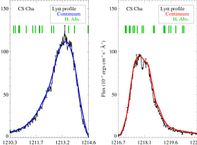
Figure 1: The stellar Ly$\alpha$ wings for one target (CS Cha) in our survey. Within the wings themselves, absorption signatures can be seen. The mean flux array over the Ly$\alpha$ profile is selected to minimize contamination from the absorption features and trace the shape of the Ly$\alpha$ wings. The mean flux array is smoothed (and shown in blue over the blue Ly$\alpha$ wing and red over the red Ly$\alpha$ wing), and the observed line profile is divided by the mean flux array to create relative absorption spectra across the Ly$\alpha$ profile. H₂ absorption transitions are identified with green hashes and properties about each transition are shown in Table 2.

2.1 COS Observations

Each PPD spectrum collected with HST/COS was taken either during the Disk, Accretion, and Outflows (DAO) of Tau Guest Observing (GO) program (PID 11616; PI: G. Herczeg) or COS Guaranteed Time Observing (PIDs 11533 and 12036; PI: J. Green). Each spectrum was observed with the medium-resolution far-UV modes of the spectrograph (G130M and G160M ($\Delta v$ $\approx$ 18 km s^-1 at Ly$\alpha$); Green et al. 2012). Multiple central wavelength positions were included to minimize fixed-pattern noise. The COS data were processed using the COS calibration pipeline (CALCOS) and were aligned and co-added with the procedure described by Danforth et al. (2010). By design, COS is a slitless spectrograph, allowing the full 2″.5 field of view through the instrument. This means the instrument is exposed to strong contamination from geocoronal Ly$\alpha$ (Ly$\alpha_{\oplus}$). To mitigate this contamination, we mask the central $\sim$ 2 Å of the Ly$\alpha$ spectra.

2.2 STIS Observations

Several targets either exceeded the COS bright-object limit or had archival STIS observations available with the desired far-UV bandpass and resolution (AB Aur, HD 104237, TW Hya). The archival data were obtained with the STIS medium-resolution grating mode (G140M ($\Delta v$ $\approx$ 30 km s^-1 between 1150 $-$ 1700 Å): Kimble et al. (1998); Woodgate et al. (1998)), while the COS-bright objects were observed with the echelle medium-resolution mode (E140M ($\Delta v$ $\approx$ 7 km s^-1 between 1150 $-$ 1700 Å)). The STIS echelle spectra were processed using echelle calibration software developed for the STIS StarCAT catalog (Ayres, 2010). Unlike COS, STIS has a small slit aperture (0″.2 $\times$ 0″.2), so the Ly$\alpha_{\oplus}$ signal is weaker; nonetheless, we remove the inner region of the Ly$\alpha$ profile ($\sim$ 0.5 $-$ 2 Å) for consistency among all the data.

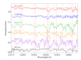
Figure 2: The normalized absorption spectra for 6 targets in our survey, ordered by increasing disk inclination angle ($i_{disk}$) from the top-down (11^∘, 34^∘, $\sim$60^∘, $\sim$70^∘, 77^∘, and 85^∘, respectively) from $\lambda\lambda$ 1217.5 $-$ 1220.5 Å. Each target is shown in a different color and offset from $I_{Ly\alpha}$ $\approx$ 1.0, which is shown with the dashed gray horizontal line. The laboratory wavelengths of H₂ absorption features considered in this study are show with solid pink vertical lines. For each target, absorption profiles are expected to be red-shifted by $v$ sin$i_{disk}$ $\approx$ 2, 0, 10, 15, 19, and 16 km s^-1, respectively (Nguyen et al., 2012; Woitke et al., 2013; Quast et al., 2000), which correspond to $\Delta\lambda$ $\sim$ 0.01, 0.00, 0.04, 0.06, 0.08, and 0.07 Å.

3 Ly$\alpha$ Normalization and Absorption Line Spectroscopy

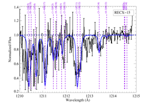
(a)

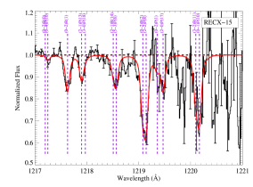
(b)

Figure 3: The best-fit H₂ absorption spectrum for RECX-15, assuming $b_{H_{2}}$ $=$ 5 km s^-1 is shown in blue (left) and red (right) over the data (black). Prominent absorption features are labeled in each figure. Table 2 lists all H₂ features considered for the fit, and Table 3 presents best-fit thermal model parameters, given the distribution of rovibrational column densities derived from these absorption line fits.

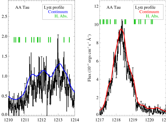
Figure 1: The Ly$\alpha$ profiles of each target, overlaid with the Ly$\alpha$ “continuum” fit determined from our functional processes (Section 3). Two targets are shown per row, where the blue and red Ly$\alpha$ profiles are presented. The Ly$\alpha$ mean flux arrays are over-plotted in blue (over the blue-wing Ly$\alpha$ component) and red (over the red-wing Ly$\alpha$ component). We mark the location of H₂ absorption transitions in the Ly$\alpha$ profiles with green hashes. The continuum fit is determined to normalize the Ly$\alpha$ emission profile, which is achieved by dividing the mean flux continuum through the emission line, creating a normalized spectral region across the Ly$\alpha$ wing.

We identify absorption signatures of H₂ in each sightline by creating transmission spectra of the stellar Ly$\alpha$ profiles of each PPD host. We treat each Ly$\alpha$ profile as a “continuum” source and normalize the emission feature, such that $I_{Ly\alpha}$ $\approx$ 1.0. We create a grid of 5 $-$ 10 unique spectral bins from $\lambda\lambda$ 1216.5 $-$ 1221.5 Å (or $\lambda\lambda$ 1210.0 $-$ 1215.0 Å for the blue wing component), which are each selected by hand to avoid molecular absorption features. Each grid bin is defined over 0.35 Å, to both smooth the Ly$\alpha$ emission feature and avoid washing out the H₂ absorption features. Within each grid, we measure the mean and standard deviation along the Ly$\alpha$ profile and store them in binned flux and error arrays. We smooth each flux array with a boxcar function of size 0.5 Å over the Ly$\alpha$ bandpass and normalize the Ly$\alpha$ profile with this smoothed grid. An example of the smoothed grid array over the Ly$\alpha$ profile for one of our survey targets is shown in Figure 1, and all Ly$\alpha$ profiles are presented in Appendix 1.

Figure 2 presents the normalized Ly$\alpha$ spectra for 6 targets, shown in order of inclination angle (edge-on targets on the bottom, and face-on targets towards the top). The effective “continuum” levels of the normalized Ly$\alpha$ flux profiles are indicated by the gray dashed lines of each spectrum, and relative flux minima with full width half maximum (FWHM) greater than the spectral resolution of the data are interpreted as absorption features. We highlight where H₂ absorption features are expected to reside in the spectrum with solid pink lines. For the edge-on targets (DF Tau, RECX-11, RW Aur), we see the absorption features appear systematically red-shifted. For face-on targets (V4046 Sgr and HD 104237), the position of the absorption features matches the expected laboratory wavelength of H₂. The observed red-shift in H₂ absorption is expected to fall within corrections made for the radial velocity ($v$ sin$i_{disk}$) of each target and the uncertainty in the COS wavelength solution ($\Delta v$ $\sim$ 15 km s^-1). Additionally, there are several absorption features seen in more than one target that do not coincide with marked H₂ features, most notably around 1218.35 Å and 1219.80 Å. As a first-order check that all H₂ and additional absorption features are not artifacts of instrument systematic errors (e.g., gain sag signature from the COS MAMA detector), we compare the Ly$\alpha$ normalized absorption profiles from two observing modes ($\lambda$1291 and $\lambda$1327) of the G130M grating for RECX-15 and find that absorption features appear in both observing modes, giving confidence that these features are real. We will attempt to identify unknown features and verify that these features are real, performing the same check on two different observing modes of COS, in Paper II.

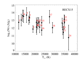
Figure 4: The rotation diagram produced for H₂ ground state rovibration levels probed in the protostellar Ly$\alpha$ profile of RECX-15. The column density in each rovibration state is determined from the H₂ absorption line fits shown in Figure 3. Each label number in the plot corresponds with the following H₂ transitions: 1. (0-2)R(1); 2. (1-2)P(4); 3. (1-2)R(5); 4. (0-1)P(10); 5. (1-1)P(11); 6. (2-2)P(8); 7. (1-1)R(12); 8. (2-1)P(13); 9. (3-1)P(14); 10. (2-1)R(14); 11. (3-2)R(11); 12. (2-0)P(17); 13. (5-3)P(8); 14. (4-2)R(12); 15. (4-1)R(16); 16. (3-0)P(18); 17. (1-5)P(3); 18. (0-4)P(10); 19. (2-5)P(11); 20. (0-3)R(19); 21. (1-4)P(14); 22. (1-4)R(17); 23. (2-4)P(18); 24. (2-5)R(15).

We create a multi-component H₂ fitting routine to measure the column density in the absorption lines probed within the red and blue stellar wings of Ly$\alpha$, pumped either into the Lyman or Werner electronic band system. We create intrinsic line profiles from the molecular transition properties (listed in Table 2) to infer the individual column densities probed in each observed rovibrational [$v$,$J$] level, as well as the average H₂ population properties (T(H₂), $b_{H_{2}}$, N(H₂)). The modeled b-value is fixed in all synthetic absorption spectra to replicate the thermal width of a warm bulk population of H₂ (T(H₂) $\geq$ 2500 K) in the absence of turbulent velocity broadening. Each line profile is co-added in optical depth space, and a transmission curve is created, which is convolved with either the COS LSF (Kriss, 2011) or a Gaussian LSF at the STIS resolving power, prior to comparison with the observed Ly$\alpha$ spectra. Each best-fit, multi-absorption feature H₂ model is then determined using the MPFIT routine (Markwardt, 2009). Initial conditions for each transmission curve were first determined by manually fitting each H₂ spectrum. To remove bias introduced by the choice of initial conditions, a grid of initial parameters was searched for all sampled absorption spectra. The only parameter allowed to float continuously for all targets was the velocity shift of the line centers of the H₂ absorption features, $v_{r}$.

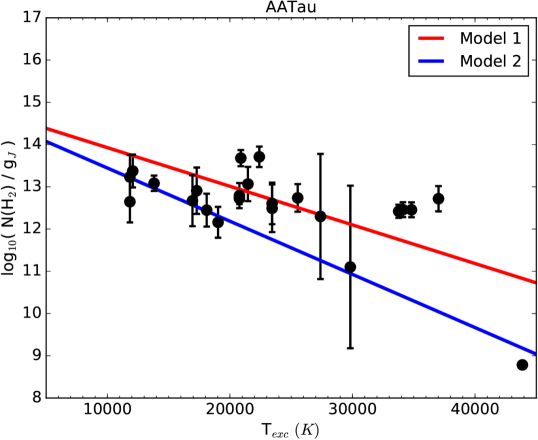
Figure 3: All rotation diagrams are presented here. Each H₂ ground state column density is weighed by its statistical weight, g_J. Model 1 attempts to fit one thermally-populated bulk H₂ population through all data points extracted from the HST data sets. Model 2 does the same as Model 1, but only for H₂ states with lower energy ground states (E_gr $\leq$ 1.5 eV; T_exc $\leq$ 17,500 K).

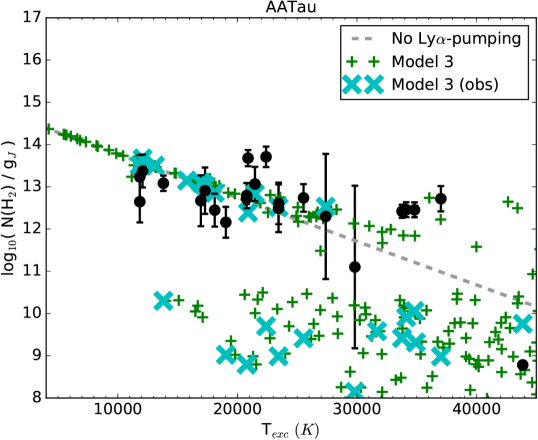
Figure 4: All rotation diagrams are presented here. Each H₂ ground state column density is weighed by its statistical weight, g_J. Model 1 attempts to fit one thermally-populated bulk H₂ population through all data points extracted from the HST data sets. Model 2 does the same as Model 1, but only for H₂ states with lower energy ground states (E_gr $\leq$ 1.5 eV; T_exc $\leq$ 17,500 K).

Figure 3 shows the normalized H₂ absorption profiles in the blue and red Ly$\alpha$ emission profiles of RECX-15, with the best-fit synthetic H₂ absorption profiles overlaid in blue (left) and red (right) and labeled with the H₂ transition information. Figure 4 presents the resulting rotation diagram of H₂ ground state rovibrational in the sightline of RECX-15. All other synthetic H₂ absorption models and rotation diagrams are presented in Figure 2. The best-fit column densities and standard deviations are plotted in rotational diagrams against the rovibrational energy level (T_exc = E^′′/k_B). Each H₂ level is statistically-weighed to correct for ortho- and para-H₂ species, such that g_J = (2S + 1)(2J + 1), for S = 0 (para-H₂) and S = 1 (ortho-H₂).

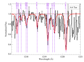
(a)

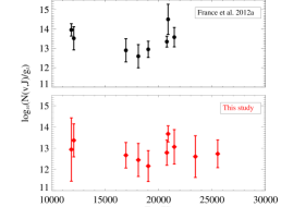
(b)

Figure 5: (a) Left: The best-fit synthetic H₂ absorption model (red) for AA Tau from 1217 $-$ 1221 Å (black). Each transition is marked with dashed purple lines and identified with the progression ID. (b) Right: We compare our column density estimates, determined from the synthetic H₂ optical depth modeling framework (red, bottom), to results from France et al. (2012a) (black, top) in H₂ rotation diagrams. Both agree within the standard deviations determined from the absorption feature analysis and show comparable temperature slopes.

We check our methodology by comparing our results to France et al. (2012a), who performed a similar procedure for the Ly$\alpha$ absorption spectrum of AA Tau. Figure 5 (left) presents the H₂ absorption spectrum for the red Ly$\alpha$ spectrum of AA Tau, as performed in this study. Figure 5 (right) shows the H₂ rotation diagram for AA Tau determined in this study (purple) and France et al. (2012a) (black). The H₂ column densities in both studies agree within the error bars determined by the multi-component fit. Our study identified two additional H₂ absorption features not fit in France et al. (2012a) (H₂[0,19], pumped by $\lambda$1217.41 Å, and H₂[6,3], pumped by $\lambda$1217.49 Å). These transitions were important to capture, as observing and characterizing high energy H₂ ground states in PPD environments is a key motivation for this study.

Table 2: Observed Ly$\alpha$-Pumped H₂ Transitions

Blue Ly$\alpha$ Wing					Red Ly$\alpha$ Wing
line ID	$\lambda_{pump}$	fosc	E′′	Aul	line ID	$\lambda_{pump}$	fosc	E′′	Aul
	(Å)	($\times$ 10-3)	(eV)	($\times$ 108 s-1)		(Å)	($\times$ 10-3)	(eV)	($\times$ 108 s-1)
B(1-2)R(5)	1210.352	36.3	1.19	1.4	C(1-5)R(5)	1216.988	7.1	2.46	0.39
C(0-3)R(19)	1210.449	25.4	2.94	1.1	C(1-5)R(9)	1216.997	19.7	2.76	0.80
B(1-2)P(4)	1210.631	29.1	1.13	1.7	B(3-3)R(2)	1217.031	1.24	1.50	0.04
C(2-5)P(11)	1210.682	30.1	2.91	1.5	B(3-3)P(1)	1217.038	1.28	1.48	0.17
C(1-4)R(17)	1211.048	37.2	3.00	1.6	B(0-2)R(0)	1217.205	44.0	1.00	0.66
C(1-5)P(3)	1211.402	7.5	2.36	0.48	C(0-4)Q(10)	1217.263	10.0	2.49	0.45
B(4-1)R(16)	1211.546	25.7	2.02	1.1	B(4-0)P(19)	1217.410	9.28	2.20	0.44
C(1-5)R(7)	1211.758	24.2	2.57	0.97	C(2-6)R(3)	1217.488	36.4	2.73	1.30
C(2-4)P(18)	1211.787	15.2	3.01	0.73	B(0-2)R(1)	1217.643	28.9	1.02	0.78
C(2-5)R(15)	1211.910	32.8	3.19	1.4	B(2-1)P(13)	1217.904	19.2	1.64	0.93
B(1-1)P(11)	1212.426	13.3	1.36	0.66	B(3-0)P(18)	1217.982	6.64	2.02	0.32
B(1-1)R(12)	1212.543	10.9	1.49	0.46	B(2-1)R(14)	1218.521	18.1	1.79	0.76
B(3-1)P(14)	1213.356	20.6	1.79	1.00	B(5-3)P(8)	1218.575	12.9	1.89	0.66
B(4-2)R(12)	1213.677	9.33	1.93	0.39	B(0-2)R(2)	1219.089	25.5	1.04	0.82
C(3-6)R(13)	1214.421	5.17	2.07	0.29	B(2-2)R(9)	1219.101	31.8	1.56	1.30
B(3-1)R(15)	1214.465	23.6	1.94	1.00	B(2-2)P(8)	1219.154	21.4	1.46	1.10
C(1-4)P(14)	1214.566	28.3	2.96	1.40	B(0-2)P(1)	1219.368	14.9	1.02	2.00
B(4-3)P(5)	1214.781	9.90	1.65	0.55	B(2-0)P(17)	1219.476	3.98	1.85	0.19
					B(0-1)R(11)	1219.745	3.68	1.36	0.15
					B(3-2)R(11)	1220.110	21.3	1.80	0.88
					B(0-1)P(10)	1220.184	5.24	1.23	0.26

4 Analysis & Results

We aim to characterize the behavior of the rovibrational H₂ populations identified in the PPD host Ly$\alpha$ spectra and estimate the total thermal and non-thermal column densities (N(H₂) and N(H₂)${}_{\textnormal{nLTE}}$) of H₂ in each sightline.

Figure 6 presents the rotation diagrams for all targets in this survey. We split the sampled sightlines by PPD evolution phase, which we define by the behavior of excess infrared (dust) emission from 13 $-$ 31 $\mu$m (Furlan et al., 2009). Primordial PPDs are thought to be disks with very little evidence of dust evolution and grain growth, meaning planet formation is either starting or in very early stages. Transitional disks are viewed as disks where proto-planets have formed and are evolving, since the observed infrared dust distributions point to the build-up of larger dust grains. Transition disks also (typically) harbor one or more large dust cavities that indicate significant evolution of the disk material (e.g., see Strom et al. 1989; Takeuchi & Artymowicz 2001; Calvet et al. 2002, 2005; Espaillat et al. 2007). To explore the behavior of H₂ populations simultaneously in all PPD sightlines, we normalize each H₂ rotation diagram to the [$v$ = 2,$J$ = 1] level. We include thermal models of warm/hot distributions of H₂ populations, drawn through the normalization rovibrational level [$v$ = 2,$J$ = 1], which range from the expected thermal populations of fluorescent H₂ in PPDs (Herczeg et al., 2002, 2006; France et al., 2012b; Hoadley et al., 2015) to the dissociation limit of the molecule (red dashed line for T_diss $\approx$ 4500 K; Shull & Beckwith 1982; Williams & Murdin 2000).

Despite the evolutionary differences in the dust distributions between the two PPD types, primordial and transitional PPD sightlines appear to show very similar H₂ rovibrational behaviors. Thermal distributions for T(H₂) $<$ 3300 K do not appear to describe the behavior of H₂ rovibration levels for T_exc $>$ 23,000 K, but a thermal distribution of H₂ at or near the dissociation limit of the molecule does appear to be consistent with the lowest column densities of rovibrational H₂ at 23,000 K $<$ T_exc $<$ 40,000 K. Still, we note that the majority of H₂ levels are significantly pumped, sometimes by as much as 4 dex, above the thermal distribution of H₂.

Additionally, we see a striking behavior in the distribution of H₂ rovibrational levels with T_exc $>$ 20,000 K. At T_exc $\sim$ 20,000 K, there is an abrupt upturn, or “knee,” away from the thermal distributions and an increase in rovibrational column density for higher excitation temperature states by $\gtrsim$ 1 dex. This “knee” appears to repeat around T_exc $\sim$ 25,500 K and 31,000-32,000 K. This behavior, specifically between the “knees” at T_exc $\sim$ 25,500 and 32,000 K, may be a result of under-sampling the distribution of highly-energetic H₂ with ground state energies in this range.

Non-thermal pumping mechanisms include many complex processes, which are challenging and computationally-expensive to model simultaneously; Nomura & Millar (2005) and Nomura et al. (2007) show how many mechanisms, such as chemical processes (resulting in the destruction and formation of H₂), FUV/X-ray pumping, and dust grain formation and size distributions in PPD atmospheres (Habart et al., 2004; Aikawa & Nomura, 2006; Nomura & Nakagawa, 2006; Fleming et al., 2010), affect the population ratios of H₂ and pump H₂ populations out of thermal equilibrium. However, Nomura & Millar (2005) also show that small changes in any of these processes can have dramatic effects on the final structure of H₂ rovibrational levels. Since we do not sample the full suite of [$v$,$J$] ground states in this absorption line study, we do not attempt to model multiple, non-thermal mechanisms in the hope of reproducing the observed behavior of H₂ rovibration levels.

Instead, we compare the observed rovibration level distributions to thermal H₂ models. While thermal models alone will not explain the distributions and behaviors of H₂ in PPD sightlines, exploring various thermal distribution realizations will help place limits on the total thermal column density of H₂ in each PPD sightline.

We fit two thermal distributions to the rovibrational levels of each target:

1. Model 1: We fit purely thermal distributions of H₂ to all observed rovibrational states, regardless of excitation temperature.

2. Model 2: We fit purely thermal distributions of H₂ to only observed rovibrational states with T_exc $\leq$ 17,500 K (E^′′ $\leq$ 1.5 eV).

We discuss the details of the molecular physics and energy equations used for Models 1 and 2 in Appendix B. Each model is optimized to the rotation diagram of each target through a Markov Chain Monte Carlo (MCMC) routine, performed with the Python emcee package (Foreman-Mackey et al., 2013). The routine uses randomly-generated initial conditions and minimizes the likelihood function of the observed rovibrational column densities, given the range of model parameters. This process determines the best representative thermal model parameters (N(H₂),T(H₂)) to the data. Further details about the MCMC and parameter fits are discussed in Appendix C.

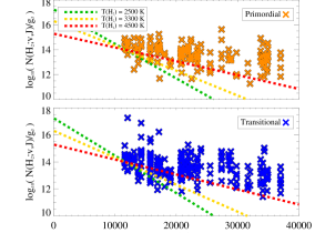
Figure 6: A relative comparison of H₂ rotation diagram behaviors. We normalize the rotation diagrams for H₂ distributions in all PPD sightlines to the [$v$ = 2,$J$ = 1] level. We split these relative spectra by disk evolution, where primordial targets are shown at the top (orange) and transitional targets are shown at the bottom (blue). We fit thermally-distributed H₂ through the [$v$ = 2,$J$ = 1] level for warm (T(H₂) = 2500 K; green) and hot (T(H₂) = 3500 K and 4500 K; yellow and red) H₂ populations.

4.1 Thermal and Non-Thermal Column Densities

Table 3: Thermal H₂ Column Density & Temperature Results

		Model 1		Model 2
Target	$v_{r}$	N(H2)	T(H2)	N(H2)	T(H2)	N(H2)${}_{\textnormal{nLTE}}$	N(H2[5,18])
AA Tau	20.1	16.27${}^{+0.50}_{-0.34}$	4179${}^{+585}_{-887}$	15.85${}^{+0.11}_{-0.11}$	3578${}^{+282}_{-221}$	16.40${}^{+0.01}_{-0.01}$	10.35
AB Aur	-12.8	15.59${}^{+0.31}_{-0.20}$	4488${}^{+376}_{-704}$	15.34${}^{+0.34}_{-0.26}$	3628${}^{+744}_{-631}$	15.44${}^{+0.01}_{-0.01}$	-
AK Sco	-4.3	15.57${}^{+0.17}_{-0.16}$	4880${}^{+90}_{-190}$	15.52${}^{+0.51}_{-0.29}$	3661${}^{+872}_{-922}$	15.04${}^{+0.05}_{-0.01}$	-
BP Tau	22.4	15.50${}^{+0.21}_{-0.19}$	4855${}^{+107}_{-220}$	15.11${}^{+0.55}_{-0.31}$	3693${}^{+868}_{-972}$	15.37${}^{+0.01}_{-0.02}$	10.72
CS Cha	13.6	15.82${}^{+0.17}_{-0.16}$	4889${}^{+83}_{-174}$	15.27${}^{+0.57}_{-0.34}$	3536${}^{+954}_{-962}$	15.52${}^{+0.01}_{-0.02}$	9.92
DE Tau	11.8	16.20${}^{+0.50}_{-0.32}$	4082${}^{+644}_{-927}$	16.08${}^{+0.86}_{-0.50}$	3466${}^{+1030}_{-1120}$	16.03${}^{+0.01}_{-0.01}$	-
DF Tau A	34.8	15.13${}^{+0.29}_{-0.19}$	4375${}^{+443}_{-695}$	14.98${}^{+0.09}_{-0.09}$	3382${}^{+188}_{-159}$	14.74${}^{+0.01}_{-0.01}$	11.19
DM Tau	40.6	16.02${}^{+0.20}_{-0.18}$	4810${}^{+140}_{-274}$	16.14${}^{+0.75}_{-0.54}$	2900${}^{+1170}_{-776}$	15.90${}^{+0.01}_{-0.02}$	10.23
GM Aur	25.4	15.84${}^{+0.18}_{-0.17}$	4873${}^{+95}_{-200}$	15.67${}^{+0.68}_{-0.50}$	2966${}^{+1096}_{-762}$	15.51${}^{+0.01}_{-0.02}$	-
HD 104237	0.6	15.95${}^{+0.27}_{-0.26}$	4831${}^{+126}_{-264}$	15.16${}^{+0.46}_{-0.28}$	3734${}^{+830}_{-906}$	16.47${}^{+0.01}_{-0.01}$	-
HD 135344 B	6.7	15.60${}^{+0.18}_{-0.17}$	4886${}^{+86}_{-181}$	15.24${}^{+0.42}_{-0.29}$	3544${}^{+878}_{-770}$	15.26${}^{+0.01}_{-0.02}$	-
HN Tau A	24.2	16.92${}^{+1.03}_{-0.64}$	3035${}^{+1193}_{-966}$	16.85${}^{+1.08}_{-0.72}$	2798${}^{+1305}_{-912}$	14.63${}^{+1.20}_{-0.20}$	-
LkCa15	35.0	17.77${}^{+0.62}_{-0.51}$	4556${}^{+324}_{-611}$	17.35${}^{+0.11}_{-0.11}$	3516${}^{+260}_{-200}$	17.64${}^{+1.50}_{-0.20}$	10.01
RECX 11	24.5	15.84${}^{+0.13}_{-0.13}$	4905${}^{+71}_{-147}$	15.55${}^{+0.24}_{-0.17}$	3939${}^{+629}_{-611}$	15.64${}^{+0.01}_{-0.01}$	9.98
RECX 15	-2.7	16.03${}^{+0.21}_{-0.20}$	4858${}^{+106}_{-219}$	15.47${}^{+0.47}_{-0.27}$	3944${}^{+729}_{-950}$	15.63${}^{+0.01}_{-0.02}$	9.48
RU Lupi	6.8	16.03${}^{+0.21}_{-0.19}$	4765${}^{+174}_{-336}$	15.38${}^{+0.61}_{-0.34}$	3840${}^{+807}_{-1106}$	15.66${}^{+0.01}_{-0.02}$	-
RW Aur A	12.4	16.23${}^{+0.29}_{-0.27}$	4822${}^{+133}_{-263}$	15.60${}^{+0.56}_{-0.33}$	3729${}^{+858}_{-1005}$	17.36${}^{+0.01}_{-0.01}$	-
SU Aur	36.0	16.21${}^{+0.51}_{-0.38}$	4264${}^{+525}_{-802}$	16.51${}^{+3.48}_{-1.22}$	2574${}^{+1654}_{-1565}$	15.31${}^{+3.00}_{-0.20}$	-
SZ 102	-20.7	15.43${}^{+0.20}_{-0.15}$	4493${}^{+362}_{-530}$	15.83${}^{+0.32}_{-0.34}$	2785${}^{+588}_{-366}$	15.26${}^{+0.01}_{-0.01}$	-
TW Hya	19.6	15.40${}^{+0.17}_{-0.16}$	4880${}^{+89}_{-192}$	15.08${}^{+0.54}_{-0.33}$	3483${}^{+954}_{-887}$	15.19${}^{+0.01}_{-0.02}$	11.31
UX Tau A	33.0	16.76${}^{+0.38}_{-0.34}$	4668${}^{+244}_{-460}$	16.40${}^{+1.32}_{-0.56}$	3129${}^{+1283}_{-1383}$	16.38${}^{+2.60}_{-0.20}$	-
V4046 Sgr	-4.7	15.33${}^{+0.15}_{-0.14}$	4894${}^{+80}_{-164}$	15.05${}^{+0.40}_{-0.25}$	3900${}^{+740}_{-891}$	15.05${}^{+0.01}_{-0.01}$	10.27
Avg. Model Results		15.97${}^{+1.80}_{-0.84}$	4604${}^{+301}_{-1570}$	15.70${}^{+1.65}_{-0.72}$	3442${}^{+500}_{-870}$

Each set of best-fit thermal model parameters is shown in Table 3. Figure 7 shows the rovibrational levels and thermal model realizations for RW Aur. We present data from this study (black circles) and lower excitation temperature states from France et al. (2014a) (black stars), which were detected against the FUV continuum between $\lambda\lambda$ 1092.5 $-$ 1117 Å. RW Aur is the only target in our sample with both sets of H₂ data and provides an example for visualizing how higher excitation temperature ground states deviate from the warm thermal levels of H₂, which are likely probing the denser regions within the disk atmosphere (log₁₀(N(H₂)) $=$ 19.90 cm^-2 and T(H₂) $=$ 440 K: magenta; France et al. 2014a). Higher energy rovibrational H₂ levels appear to scatter out of thermal equilibrium and are described by higher effective temperatures, as predicted by Nomura & Millar (2005). We present all H₂ rotation diagrams and thermal distribution realizations for each target in our survey in Appendix 4.

Table 2 lists the average S/N of each Ly$\alpha$ emission profile as observed by either HST/COS or HST/STIS. We compute a Spearman rank coefficient between the best-fit thermal model N(H₂) and the Ly$\alpha$ wing S/N and find significant trends for both Model 1 ($\rho$ = -0.71, with a probability to exceed the null hypothesis that the data are drawn from random distributions (p = 7.0$\times$10^-3) and Models 2 ($\rho$ = -0.78, p = 5.6$\times$10^-2). However, when we exclude one low S/N data point from the correlation (LkCa 15) and re-calculate the Spearman rank coefficient for both model realizations, we see a more randomly-distributed set of modeled column density estimates (Model 1: $\rho$ = -0.22, p = 3.91$\times$10^-1 and Model 2: $\rho$ = -0.27, p = 1.92$\times$10^-1). Therefore, for the remainder of this study, we do not include LkCa 15 results in further analysis.

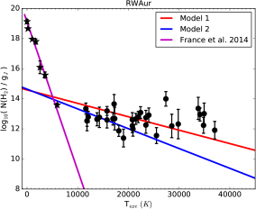
Figure 7: The rotation diagram for RW Aur, with rovibrational column densities derived in this study (black circles) and lower energy states measured by France et al. (2014a) (black stars; $\lambda\lambda$ 1092.5 $-$ 1117 Å). The red and blue solid lines represent thermal distributions of H₂ levels populated in Models 1 and 2, respectively. The magenta solid line shows the thermal distribution H₂ levels examined by France et al. (2014a), with log₁₀( N(H₂) ) $=$ 19.90 cm^-2 and T(H₂) $=$ 440 K.

We use the results from Models 1 and 2 to estimate the total column density of thermally-distributed H₂ (N(H₂)) in each sight line. We choose to represent the thermal distributions of hot H₂ with the results from Model 2. T(H₂) from Model 2 represents a more realistic determination of the bulk temperature profiles of thermal H₂ (T(H₂) $\sim$ 2500 $-$ 3500 K) in each sightline, whereas Model 1 produces T(H₂) $\approx$ T_diss(H₂). In reality, there is very little difference between N(H₂) determined from Models 1 and 2; both model realizations predict similar N(H₂), though Model 2 results tend to under-predict N(H₂) when compared to Model 1 results, and thus provide a lower limit to the total thermal column density of hot H₂.

To approximate how much of the total observed H₂ column density is associated with excess H₂ populations in highly energetic (non-thermal) states, we define a metric for the total non-thermal column density of H₂ in highly excited levels (E^′′ $>$ 1.75 eV, or T_exc $>$ 20,000 K), which we refer to as N(H₂)${}_{\textnormal{nLTE}}$. N(H₂)${}_{\textnormal{nLTE}}$ is calculated by integrating the residual between observed H₂ rovibration levels with T_exc $>$ 20,000 K and the predicted populations of H₂ at that same rovibration level from the modeled thermal distributions, or N(H₂)${}_{\textnormal{nLTE}}$ = $\Sigma_{[v,J]}($N(H₂[$v$,$J$])${}_{\textnormal{obs}}$ - N(H₂[$v$,$J$])${}_{\textnormal{model}})$. For consistency, we calculate N(H₂)${}_{\textnormal{nLTE}}$ from all best-fit model realizations from both Models 1 and 2. We find we are able to produce approximately the same N(H₂)${}_{\textnormal{nLTE}}$ estimate from N(H₂) of both Models 1 and 2. Associated error bars on N(H₂)${}_{\textnormal{nLTE}}$ are estimated as the minimum and maximum deviations away from the median N(H₂)${}_{\textnormal{nLTE}}$ for all Model 1 and Model 2 best-fit thermal parameters. Table 3 includes our estimates of N(H₂)${}_{\textnormal{nLTE}}$ for each target (for which we include LkCa 15, but we do not use in further analysis).

4.2 C IV-Pumped H₂ Fluorescence

Molecular hydrogen populations photo-excited by C IV photons ($\lambda$ 1548.20, 1550.77 Å) are found in highly excited ground states ([3,25], [5,18], and [7,13]; E^′′ $\geq$ 3.8 eV, T_exc $>$ 43,000 K) that are difficult to explain with thermally-generated H₂ populations alone. These highly excited states are also unlikely to be directly populated by the fluorescence process. Electronic transitions are dipole-allowed, meaning $J^{\prime}-J^{\prime\prime}$ = $\pm$1 or 0 (for Werner band lines with $J^{\prime\prime}$ $\neq$ 0) between excited and ground state transitions. The decay from excited electronic to ground states can easily increase the ground electronic vibrational levels, but will not substantially change the ground electronic quantum rotational levels (Herczeg et al., 2006). Therefore, other physical mechanisms, such as collisional (Bergin et al., 2004) and chemical (Takahashi et al., 1999; Ádámkovics et al., 2016) processes, must be responsible for populating these highly energetic levels of H₂.

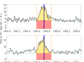
Figure 8: The presence of C IV-pumped H₂ emission from the B(0-5)P(18) progression. We present example fluorescence lines for BP Tau, for emission lines at 1501.75 Å ((0-5)R(16)) and 1554.95 Å ((0-6)R(16)), indicated by the blue dotted lines. The green dashed line shows the continuum levels in each spectral region. The orange dashed lines mark off the region considered for each fluorescence line. The yellow hashed region represents the integrated flux F(C IV-H₂) within the orange region, while the red hashed region represents the integrated continuum flux in the same region.

Since we do not know which processes dominate the pumping of H₂ into these highly energetic upper rotational levels, we use the emission from C IV-pumped H₂ as a proxy for a variety of non-thermal processes that may excite H₂ to highly non-thermal states. We estimate the column density of H₂ populating these energetic levels from the total fluorescent emission produced by C IV-pumped H₂. We stipulate two conditions to verify whether the target exhibits C IV-pumped H₂ emission in the FUV spectrum: 1) each emission line must have an elevated flux level $\geq$ 1.5$\sigma$ above the continuum floor, and 2) at least two emission lines from the same progression must be present. Figure 8 demonstrates how we determine that the emission line exists above the FUV continuum. Only fluorescence from the B(0-5)P(18) 1548.15 Å transition meets this criteria for targets which show signs of C IV-pumped H₂ emission in our survey. The two brightest transitions from the B(0-5)P(18) 1548.15 Å cascade, $\lambda$ 1501.75 Å and $\lambda$ 1554.95 Å, are free of blending from other atomic or molecular contaminants (Herczeg et al., 2006). Therefore, emission features observed at these wavelengths are detected fluorescence transitions, originating from the highly non-thermal H₂ state [5,18]. Of the 22 targets, 10 show statistically significant emission lines from C IV-pumped H₂ fluorescence.

To estimate the density of highly excited H₂, we use the flux from the two brightest emission features at $\lambda$ 1501.75 Å and $\lambda$ 1554.95 Å, after subtracting the UV continuum. We assume that H₂[5,18] is optically thin and estimate the total column density of this highly non-thermal ground state (N(C IV-H₂)) from the formalism described in Rosenthal et al. (2000),

where N(C IV$\rightarrow$H₂[$v^{\prime\prime}$,$J^{\prime\prime}$]) is the column density of C IV-pumped H₂ that decays to ground state [$v^{\prime\prime}$,$J^{\prime\prime}$], $\lambda$ is the transition wavelength between electronic and ground states, F(C IV-H₂) is the integrated flux in the emission line produced by the transition between excited electronic level [$v^{\prime}$,$J^{\prime}$] and ground level [$v^{\prime\prime}$,$J^{\prime\prime}$], and $A_{ul}$ is the spontaneous decay rate for the transition. For each emission line, we calculate N(C IV-H₂) and take the average of the results from the two emission features as the estimate of N(C IV-H₂). Error bars on N(C IV-H₂) are taken as the residual between the N(C IV-H₂) and the column density derived from each emission feature at $\lambda$ 1501.75 Å and $\lambda$ 1554.95 Å. Derived N(C IV-H₂) values are listed in Table 3. All column densities derived from the fluorescence emission from the B(0-5)P(18) progression are log₁₀(N(C IV-H₂)) $<$ 12.0 cm^-2, which is consistent with a thin layer of highly energetic H₂ (Herczeg et al., 2006).

5 Discussion

This study has focused on characterizing the column density of H₂ from observed distributions of rovibrational states derived from their respective absorption features embedded within the stellar Ly$\alpha$ wings of PPD hosts. We discovered that we systematically find higher excitation levels with larger column densities than expected from thermally-distributed, warm populations of H₂. The observed H₂ distributions of rovibrational states tells us that some mechanism or mechanisms in and/or around the circumstellar environment is/are affecting the equilibrium state of warm molecules in these sightlines. We aim to characterize the general behavior of thermal and non-thermal H₂ populations and column densities in PPD environments by comparing these quantities to stellar and circumstellar observables.

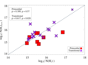
(a)

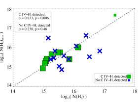
(b)

Figure 9: We compare model-derived N(H₂) to N(H₂)${}_{\textnormal{nLTE}}$ and separate populations by disk evolutionary phase (left) and whether there is evidence of C IV-pumped H₂ fluorescence in the FUV spectrum (right). Transitional disk targets and targets with detected C IV-pumped H₂ fluorescence (AA Tau, BP Tau, CS Cha, DF Tau, DM Tau, LkCa 15, RECX 11, RECX 15, TW Hya, and V4046 Sgr) appear to have direct correlations with N(H₂) $\sim$ N(H₂)${}_{\textnormal{nLTE}}$.

First, we look for correlations between the modeled distributions of warm, thermal H₂ (T(H₂) $>$ 2500 K) and the populations of non-thermal H₂ states for the sampled PPD sightlines. Figure 9 compares thermal, model-derived N(H₂) to the sum of the residuals in highly-energetic H₂ states, N(H₂)${}_{\textnormal{nLTE}}$. Before noting the distributions of total column densities by categorization, we see that the general trend between the distributions of N(H₂) and N(H₂)${}_{\textnormal{nLTE}}$ appear roughly related, with a Spearman rank coefficient which agrees with this assessment ($\rho$ = +0.54), but a PTE that suggests there is no strong indication of a trend between the two variables (p = 1.17$\times$10^-1). However, when we categorize targets by their disk evolution and whether C IV-pumped H₂ fluorescence is detected in their FUV spectra, we see much clearer trends that point to target distributions which have correlated N(H₂) and N(H₂)${}_{\textnormal{nLTE}}$ populations. Transitional disks appear to predominantly straddle the N(H₂) = N(H₂)${}_{\textnormal{nLTE}}$ equality line ($\rho$ = +0.62, p = 2.00$\times$10^-2), and targets which have detectable C IV-pumped H₂ fluorescence show the same behavior ($\rho$ = +0.83, p = 6.03$\times$10^-3). Primordial disk targets appear to have more scattered distributions of N(H₂) and N(H₂)${}_{\textnormal{nLTE}}$ ($\rho$ = +0.31, p = 5.69$\times$10^-1), as do targets with no detected C IV-pumped H₂ fluorescence ($\rho$ = +0.24, p = 4.82$\times$10^-1).

5.1 H₂ Column Densities & the Circumstellar Environment

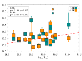
(a)

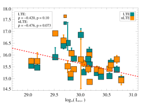
(b)

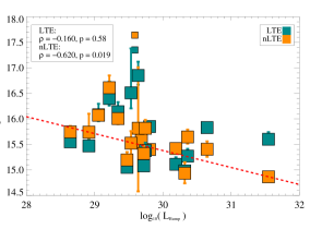
(c)

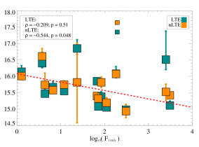
(d)

Figure 10: We compare the total column densities of thermal and non-thermal H₂ to the total X-ray luminosity (top left), the total FUV continuum luminosity (top right), the total H₂ dissociation “bump” luminosity around $\lambda$ 1600 Å (bottom left), and the integrated flux from $\lambda\lambda$ 912 $-$ 1150 Å (bottom right). N(H₂) shows no significant correlations with any high-energy radiation observables, while N(H₂)${}_{\textnormal{nLTE}}$ shows confident trends with L_X, L_Bump, and F${}_{1110\textnormal{\AA}}$. Both total column densities show a very loose trend with L_FUV. Outside of log space, the column density variables have units of cm^-2, the luminosity variables have units of erg s^-1, and the flux variables have units of erg cm^-2 s^-1.

We first consider the role of excess FUV and X-ray emission on the modeled thermal and non-thermal total column densities of H₂, to explore if the distributions of observed H₂ levels match the behaviors observed in Nomura & Millar (2005) and Nomura et al. (2007). We split the various excess emission into the following categories: the total X-ray luminosity (L_X; France et al. 2017 and references therein), the total FUV continuum luminosity (L_FUV: $\lambda\lambda$ 1490 $-$ 1690 Å, excluding any discrete or extended emission features; France et al. 2014b), the total H₂ dissociation continuum around $\lambda$ 1600 Å (L_Bump; France et al. 2017), and the total observed flux, corrected for ISM reddening, of FUV continuum+discrete emission features from $\lambda\lambda$ 912 $-$ 1150 Å (F${}_{1110\textnormal{\AA}}$; France et al. 2014b). Figure 10 shows the comparison of N(H₂) and N(H₂)${}_{\textnormal{nLTE}}$ to these circumstellar observables. We note a correlation between L_X and N(H₂)${}_{\textnormal{nLTE}}$ ($\rho$ = +0.53, p = 4.00$\times$10^-2), but no correlation between N(H₂) and L_X ($\rho$ = +0.15, p = 6.62$\times$10^-1). We observe an anti-correlation between N(H₂)${}_{\textnormal{nLTE}}$ and L_Bump ($\rho$ = -0.62, p = 1.90$\times$10^-2) and no strong trend between N(H₂) and L_Bump ($\rho$ = -0.16, p = 5.83$\times$10^-1). We again find an anti-correlation between N(H₂)${}_{\textnormal{nLTE}}$ and F${}_{1110\textnormal{\AA}}$ ($\rho$ = -0.54, p = 4.81$\times$10^-2), yet no indication of a trend between N(H₂) and F${}_{1110\textnormal{\AA}}$ ($\rho$ = -0.21, p = 5.14$\times$10^-1). Finally, both N(H₂) and N(H₂)${}_{\textnormal{nLTE}}$ show suggestive anti-correlations with L_FUV, but they are not statistically significant (N(H₂): $\rho$ = -0.42, p = 1.02$\times$10^-1; N(H₂)${}_{\textnormal{nLTE}}$: $\rho$ = -0.48, p = 7.30$\times$10^-2).

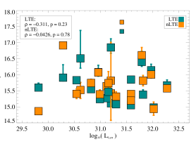
(a)

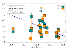
(b)

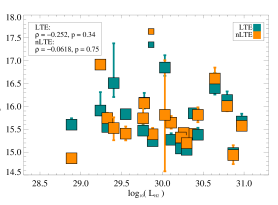
(c)

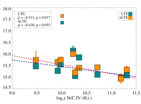
(d)

Figure 11: We compare the total column densities of thermal and non-thermal H₂ to the total Ly$\alpha$ luminosity (top left), the total C IV luminosity (top right), the total H₂ fluorescence luminosity (bottom left), and the total column density of H₂ found in H₂[5,18] (bottom right). N(H₂) shows confident trends with L_CIV and N(C IV-H₂), while N(H₂)${}_{\textnormal{nLTE}}$ only displays a loose trend with N(C IV-H₂). We find no correlations between the modeled H₂ column densities and L_Lyα and L${}_{H_{2}}$. Outside of log space, the column density variables have units of cm^-2 and the luminosity variables have units of erg s^-1.

Next, we look at how discrete emission line features (from the protostar and accretion shock regions) and disk fluorescence processes may play a role on the total column densities of H₂ in PPD sightlines. We split the circumstellar parameters into the following categories: the total luminosity from stellar+shock-generated Ly$\alpha$ emission (L_Lyα; ; France et al. 2014b), the total luminosity from stellar+shock-generated C IV emission (L_CIV; France et al. 2014b), the total H₂ fluorescence luminosity from Ly$\alpha$-pumped H₂ predominantly produced in the disk atmosphere (L${}_{H_{2}}$; France et al. 2014b), and the estimated total column density of H₂[5,18], derived from the statistically-determined C IV-pumped fluorescence features (N(C IV-H₂), derived in Section 4.2). Figure 11 shows the comparison of N(H₂) and N(H₂)${}_{\textnormal{nLTE}}$ to these circumstellar variables. We find no trends between the modeled column densities of H₂ and L_Lyα (N(H₂): $\rho$ = -0.31, p = 2.34$\times$10^-1; N(H₂)${}_{\textnormal{nLTE}}$: $\rho$ = -0.04, p = 7.86$\times$10^-1), as well as L${}_{H_{2}}$ (N(H₂): $\rho$ = -0.25, p = 3.45$\times$10^-1; N(H₂)${}_{\textnormal{nLTE}}$: $\rho$ = -0.06, p = 7.54$\times$10^-1). We do see a suggestive anti-correlation between L_CIV and N(H₂) ($\rho$ = -0.51, p = 4.52$\times$10^-2), but no trend between N(H₂)${}_{\textnormal{nLTE}}$ and L_CIV ($\rho$ = -0.19, p = 5.62$\times$10^-1). Finally, we find anti-correlated behavior between both N(H₂) and N(H₂)${}_{\textnormal{nLTE}}$ with N(C IV-H₂) (N(H₂): $\rho$ = -0.51, p = 1.71$\times$10^-2; N(H₂)${}_{\textnormal{nLTE}}$: $\rho$ = -0.43, p = 5.50$\times$10^-2).

5.2 The Behavior of Hot H₂

We find that the column densities of H₂ are correlated to many non-thermal diagnostics of the circumstellar environment, such as internal radiation and H₂ dissociation tracers. The observed distribution of H₂ absorption populations appear to be located somewhere in the disk environment where 1) 1) the H₂ have access to protostellar radiation with $\lambda$ $<$ 1110 Å, and 2) the H₂ populations are optically-thin to Ly$\alpha$ radiation. Piecing our results together, we suspect that the observed H₂ populations against the protostellar Ly$\alpha$ wing provide are not associated with the H₂ that fluoresces in the disk and may, instead, arise from a hot, tenuous disk halo. Ádámkovics et al. (2016) explore the effects of FUV, X-ray, and Ly$\alpha$ radiation on stratified layers of molecular PPD atmospheres. In the presence of all three, FUV continuum and X-ray radiation create a hot, atomic layer along the uppermost disk surface, and Ly$\alpha$ radiation penetrates deeper into the disk via H I scattering. The penetration of Ly$\alpha$ into the molecular disk is found to photodissociate trace molecules like H₂O and OH, which, along with H₂ formation on dust grains, heat this region of the disk and create a warm molecular layer (T_gas $>$ 1500 K). This warm layer is found to have an appreciable column of warm H₂ (N(H₂) $>$ 10¹⁹ cm^-2) in the appropriate temperature regime to reproduce fluorescent emission signatures in PPDs, though the distribution of H₂ rovibrational levels is not computed in the Ádámkovics et al. (2016) models.

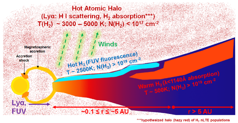
Figure 12:

The Ádámkovics et al. (2016) study produces a hot (T $\sim$ 5000 K) atomic layer in the uppermost disk atmosphere, which is similar in nature to a photodissociation region (PDR; Hollenbach & Tielens 1999 and references therein). This hot atomic layer is produced in all of their model parameter space, independent of stellar Ly$\alpha$ luminosity or dust grain distributions. This layer of hot atomic gas contains a minute abundance of H₂ ($x$(H₂) $\lesssim$ 10^-5) with total column densities of hot H₂ similar to those found in this study (N(H₂)_hotlayer $\sim$ 10¹⁵ cm^-2; $\langle$N(H₂)${}_{H_{2}abs}\rangle$ $\sim$ 10^15.5 cm^-2). This hot atomic layer is modeled above the warm molecular layer (where H₂ fluorescence may arise) and extends substantially further away from the disk midplane (Ádámkovics et al., 2016). What their study finds is that Ly$\alpha$ radiation is key to producing the warm molecular regions that may be associated with warm H₂ and CO populations, but the hot, atomic layer is driven by the FUV continuum and X-ray luminosities, which cannot penetrate into the cooler disk like Ly$\alpha$ can.

Connecting the findings from this work and the Ádámkovics et al. (2016) models, we suggest that the observed H₂ absorption populations, probed in the wings of protostellar Ly$\alpha$ profiles, reside in this tenuous, hot atomic region of the circumstellar environment. We argue that the behavior of the Ly$\alpha$ transition, being by nature a powerful resonance line, allows Ly$\alpha$ radiation to scatter through both the PPD and the surrounding PDR-like environment. Rather than probing a discrete line source coming straight from the accretion shock near the protostellar surface, we probe Ly$\alpha$ that has scattered through the circumstellar environment by H I atoms before reaching the observer. The scattering of Ly$\alpha$ radiation by H I, which occurs when a Ly$\alpha$ photon is absorbed and emitted many times into many different directions and results in changes in the frequency of Ly$\alpha$ away from rest wavelength, causes significant broadening of the Ly$\alpha$ profile on order of several hundred km s^-1 before escaping the star (see McJunkin et al. 2014 for a more complete overview of this process). It appears that the H₂ probed in absorption against these observed Ly$\alpha$ wings may be tied to this optically-thin, hot halo surrounding the PPD, where optically-thin densities of H₂ absorb Ly$\alpha$ before it can exit the system.

5.2.1 H₂ “Multiple Pumping” Versus Cooling

The scattering of Ly$\alpha$ radiation through the hot atomic regions surrounding PPDs may help explain the non-thermal behavior of H₂ associated with these environments. The behavior of the observed rovibrational levels may be the result of “multiple pumping” happening with the hot H₂, meaning that the excitation rate by UV photon absorption (in this case, specifically Ly$\alpha$ photons) is faster than the molecules can decay (cool) via rovibrational emission lines or collisions.

We perform a back-of-the-envelope comparison of the H₂ rovibrational emission and total collision rates required to balance H₂ photo-excitation (“Ly$\alpha$-pumping”), assuming the H₂ species are located in a hot atomic layer above the PPD. The hot atomic region is assumed to be a plane-parallel slab above the inner disk ($r$ $<$ 1 AU; Ádámkovics et al. 2016) with a thickness $a$ $\sim$ 1 AU. We assume the average Ly$\alpha$ luminosity for a typical PPD system $\langle$L${}_{Ly\alpha}\rangle$ $\sim$ 10³¹ erg s^-1 (Schindhelm et al., 2012; France et al., 2014b), which translates into an average photon rate $\langle\Gamma_{Ly\alpha}\rangle$ = $\langle$L${}_{Ly\alpha}\rangle$ / E_Lyα $\sim$ 10⁴² photons s^-1 incident on the hot H₂. Since H₂ is expected to only be a trace species in this region ($x$(H₂) $\sim$ 10^-5; Ádámkovics et al. 2016), we include a “coverage factor” for the total Ly$\alpha$ luminosity on the H₂ populations. This leads to an estimation of the total photo-excitation rate of H₂ in the hot atomic layer, $\langle\Gamma_{Ly\alpha}\rangle$ $\sim$ $x$(H₂)$\times$10⁴² photons s^-1 $\sim$ 10³⁷ photons s^-1. We calculate the average rate of incident Ly$\alpha$ photons on the H₂ populations in the PDR slab to be $\gamma_{Ly\alpha}$ $\sim$ $\langle\Gamma_{Ly\alpha}\rangle$ / ($\sigma$(H₂)$\times a^{2}$) $\approx$ 10^-3 photon s^-1, where $\sigma$(H₂) is the average Ly$\alpha$ line absorption cross-section of an individual molecules, given by

$$\sigma(H_{2})=\frac{\sqrt{\pi}e^{2}}{m_{e}cb_{H_{2}}}\lambda_{i}f_{i}$$ (2)

(McCandliss, 2003; Cartwright & Drapatz, 1970), where $\lambda_{i}$ is the absorption wavelength for a given transition in the Ly$\alpha$ profile (taken as 1215.67 Å for this example), $f_{i}$ is the oscillator strength (the average assumed as $\approx$0.01), and $b_{H_{2}}$ is the b-value of the line, assumed to match our models ($b_{H_{2}}$ = 5 km s^-1), producing an average cross section for Ly$\alpha$ photon absorption $\sigma$(H₂) $\sim$ 10^-14 cm².

We do not include additional losses of Ly$\alpha$ flux due to absorption from other atomic species, as it is assumed that the dominant constituent of the disk PDR is neutral hydrogen at an average $T_{gas}$ $\sim$ 3500 - 5000 K, which will scatter Ly$\alpha$ around the region. We can quantify the ratio of the UV photo-excitation rate to the average transition probability for quadrupolar H₂ IR emission lines ($A_{quad}$ $\sim$ 10^-7 s^-1; Wolniewicz et al. 1998), $\gamma_{Ly\alpha}$ / $A_{quad}$ $\sim$ 10⁴ photons, meaning that of order 10,000 Ly$\alpha$ photons are absorbed for every one quadrupolar photon emitted. Therefore, quadrupole emission is not an effective means of cooling the photo-excited H₂ populations in these regions.

Next, we explore what the expected collisional rate between H₂ and other particles in the hot atomic slab must be to balance with the UV photo-excitation rate. First, we set the total collisional rate of all particle interactions with H₂ in this region to match the photo-excitation rate of H₂ in the hot atomic region, such that $\Sigma\alpha_{H_{2},i}$ = $\gamma_{Ly\alpha}$ $\sim$ 10^-3 collisions s^-1. Given $\langle$N(H₂)$\rangle$ from our empirical models, we estimate the total number density of H₂ in the hot atomic layer to be $n$(H₂) $\sim$ 10³ cm^-3. Finally, we estimate the total collisional rate with H₂ needed to match the photo-excitation rate of H₂ via Ly$\alpha$-pumping, $\Sigma C_{H_{2},i}$ $\sim$ $\Sigma\alpha_{H_{2},i}$ / $n$(H₂) $\sim$ 10^-6 cm³ s^-1.

This result suggests that, at T_gas $\approx$ 3500 - 5000 K, interactions between H₂ and dominant particles in the hot atomic environment, like H I, protons (p⁺), and electrons (e^-), are expected to occur at a total rate of $\sim$10^-6 cm³ s^-1. Mandy & Martin (1993) and Roberge & Dalgarno (1982) find collisional rates between H₂ + H I to be of order $C_{H_{2},HI}$ $\sim$ 10^-10 cm³ s^-1 for gas with T_gas $\approx$ 2000 - 4500 K (which is similar to interactions between H₂ + p⁺; Black & Dalgarno 1977; Smith et al. 1982). The rate of collisions between H₂ + e^-, for gas with T_gas $\sim$ 3500 K, is found to be $C_{H_{2},e^{-}}$ $\sim$ 10^-11 cm³ s${-1}$ (Prasad & Huntress, 1980). Additionally, interactions between H₂ + H₂ are expected to occur much less frequently, with $C_{H_{2},H_{2}}$ $\sim$ 10^-16 cm³ s${-1}$ for $T_{gas}$ $\sim$ 3500 K (Mandy, 2016).

We find that the integrated collision rate of H₂ in these environments, derived from literature values, is $\sim$ 4 dex lower than the photo-excitation rate of H₂ by Ly$\alpha$ radiation alone. When we quantify the ratio of the UV photo-excitation rate to the total collisional rate of particles with H₂ in this exercise (optimistically assuming $\Sigma C_{H_{2},i}$ $\sim$ 10^-9 cm³ s^-1), $\gamma_{Ly\alpha}$ / ( $\Sigma C_{H_{2},i}\times n$(H₂) ) $\sim$ 10³ photons, or that $\sim$1,000 Ly$\alpha$ photons are absorbed for every one de-excitation collision of H₂.

We conclude that is it therefore plausible that ”Ly$\alpha$ multiple pumping” may play a key role in re-distributing H₂ rovibrational states in this hot gas region of the circumstellar environment before collisions or rovibrational emission can cool the molecules. Indeed, our simple calculation compliments observed behaviors of H₂ rovibration levels in ISM PDR environments (e.g., Draine & Bertoldi 1996; Hollenbach & Tielens 1999, and references therein). The critical density of most H₂ rovibration levels, or the ratio of the radiative lifetime of a given state ($A_{ul}$, in s^-1) to the collision rate for de-excitation out of the same state ($C_{H_{2},i}$, in cm³ s^-1), is typically of order 10⁴ cm^-3 for $T_{gas}$ $>$ 2000 K (Mandy & Martin, 1993). In our estimation, the density of H₂ is near this critical density, but is still under it, allowing “multiple pumping” to populate H₂ states by UV pumping before collisions de-excite the level populations (Draine & Bertoldi, 1996; Hollenbach & Tielens, 1999).

5.2.2 A Simple Model of Ly$\alpha$-pumped H₂

What, then, is the expected distribution of H₂ rovibration levels if Ly$\alpha$-pumping plays a significant role in regulating the ground states of the molecules? We create a simple model of H₂ photo-excitation, in the absence of cooling routes (i.e., rovibrational emission and collisional de-excitation), which tracks the column densities of individual H₂ rovibrational levels in the presence of an appreciable Ly$\alpha$ radiation field. This model tracks the fluorescence cascade of H₂ from excited electronic levels, pumped by photo-excitation, back to the ground electronic level until the column densities of rovibration states settles to a preferential distribution, (i.e. the states no longer significantly change due to the photo-excitation process). The framework of the model, which we will refer to as Model 3, is as followings:

1. We start with a thermal distribution of hot H₂, where rovibrational levels are statistically defined by the total column density (N(H₂)) and temperature (T(H₂)) of the bulk molecular population.

2. A constant, uniform radiation distribution of Ly$\alpha$ photons are generated and exposed to the initially-defined thermal population of H₂.

3. H₂ in the correct [$v$,$J$] ground level will have some probability to absorb Ly$\alpha$ photons incident on the H₂ populations. If the H₂ molecules absorb the photons, they are pumped to an excited electronic level, either in the Lyman or Werner bands. From there, they immediately decay back to the ground state in a fluorescent cascade. The probability for a Ly$\alpha$-pumped H₂ to decay back to a specific ground level is defined by the branching ratios (transition probabilities) from the excited electronic level [$v^{\prime}$,$J^{\prime}$] to the ground electronic level [$v^{\prime\prime}$,$J^{\prime\prime}$].

4. All rovibration levels of H₂ are followed simultaneously and allowed to redistribute themselves by transition probabilities after initially being photo-pumped out of their original ground electronic level, [$v$,$J$]. The model runs until the ground rovibration levels settle to a nearly constant distribution of levels in the presence of this unchanging Ly$\alpha$ radiation field.

The Ly$\alpha$ radiation distribution used in Model 3 is assumed to mimic the observed line width and shape on a target-by-target basis. The Ly$\alpha$ line shape is assumed to be Gaussian, with parameters describing the line shape adapted from McJunkin et al. (2014). The flux in the Ly$\alpha$ line, $F_{Ly\alpha}$, is allowed to float in each model run, as are N(H₂) and T(H₂), which set the initial conditions for each model iteration. For the duration of each model, the Ly$\alpha$ line emission is assumed to neither change in shape nor in peak flux, effectively providing the H₂ populations with a constant, uniform distribution of Ly$\alpha$ photons until the H₂ ground states relax to some preferential distribution. The basic mechanics of the model take advantage of $\sim$100 H₂ cross sections coincident with the Ly$\alpha$ emission profiles of typical PPD targets (i.e., Classic T Tauri stars; France et al. 2014b). These cross sections are calculated using intrinsic transition properties of H₂ with Ly$\alpha$ provided by Abgrall et al. (1993a) and Abgrall et al. (1993b). Based on the energy of a given Ly$\alpha$ photon, H₂ in a receptive rovibration level [$v$,$J$] will absorb the photon and be pumped to either the Lyman or Werner excited electronic band. The excited H₂ molecules will decay back to one of many potential ground electronic rovibration levels via branching ratio probabilities, again inferred from intrinsic molecular properties provided by Abgrall et al. (1993a) and Abgrall et al. (1993b). This process is repeated until the rovibration levels of H₂ relax to some distribution of states under the constant Ly$\alpha$ flux (i.e., no significant change in the column densities of rovibration levels is detected, to within $\delta$log₁₀N(H₂[$v$,$J$]) $\lesssim$ 0.1 for all rovibration levels). See Appendix C.1 for more details about the models, including the iteration process used for Ly$\alpha$-pumping, H₂ electronic fluorescence and further details regarding the MCMC and statistics of the process.

Table 4: Ly$\alpha$-pumped H₂ Column Density & Temperature Results

	Model 3
Target	N(H2)	T(H2)	FLyα	$\Delta$N(H2)
AA Tau	16.28${}^{+0.52}_{-0.33}$	3214${}^{+570}_{-810}$	-10.4${}^{+0.8}_{-0.7}$	14.13
AB Aur	15.60${}^{+0.29}_{-0.16}$	3437${}^{+410}_{-691}$	-10.5${}^{+0.5}_{-0.6}$	13.44
AK Sco	15.65${}^{+0.50}_{-0.27}$	3601${}^{+290}_{-522}$	-10.2${}^{+0.7}_{-0.3}$	13.35
BP Tau	17.09${}^{+0.94}_{-0.58}$	2557${}^{+1113}_{-1339}$	-6.7${}^{+0.6}_{-0.5}$	13.09
CS Cha	18.36${}^{+0.68}_{-1.17}$	1596${}^{+1700}_{-340}$	-6.9${}^{+0.3}_{-0.4}$	13.61
DE Tau	16.21${}^{+0.45}_{-0.34}$	2982${}^{+693}_{-812}$	-9.4${}^{+0.7}_{-0.7}$	13.94
DF Tau A	16.48${}^{+1.23}_{-1.38}$	2678${}^{+940}_{-1258}$	-6.9${}^{+0.4}_{-4.2}$	12.63
DM Tau	16.30${}^{+0.80}_{-0.28}$	3670${}^{+232}_{-888}$	-8.7${}^{+1.0}_{-0.6}$	13.90
GM Aur	16.15${}^{+0.32}_{-0.22}$	3469${}^{+376}_{-650}$	-7.5${}^{+0.3}_{-0.4}$	13.55
HD 104237	17.87${}^{+0.57}_{-0.52}$	2200${}^{+1060}_{-766}$	-5.7${}^{+0.2}_{-0.3}$	13.25
HD 135344 B	16.78${}^{+0.46}_{-0.31}$	3185${}^{+517}_{-1128}$	-6.4${}^{+0.3}_{-0.3}$	13.26
HN Tau A	16.95${}^{+0.99}_{-0.64}$	2140${}^{+1088}_{-998}$	-8.9${}^{+1.5}_{-1.3}$	12.24
LkCa15	18.09${}^{+1.00}_{-0.53}$	3456${}^{+394}_{-858}$	-8.9${}^{+2.1}_{-1.3}$	13.81
RECX 11	16.72${}^{+0.32}_{-0.25}$	3087${}^{+593}_{-411}$	-6.7${}^{+0.3}_{-0.7}$	13.60
RECX 15	17.13${}^{+0.55}_{-0.53}$	2679${}^{+933}_{-798}$	-5.9${}^{+0.2}_{-0.5}$	13.85
RU Lupi	17.26${}^{+0.46}_{-0.47}$	2735${}^{+621}_{-976}$	-5.7${}^{+0.1}_{-0.4}$	13.95
RW Aur A	18.03${}^{+0.68}_{-0.71}$	2504${}^{+1489}_{-627}$	-5.6${}^{+0.1}_{-0.2}$	14.25
SU Aur	17.59${}^{+1.31}_{-1.20}$	2739${}^{+857}_{-1631}$	-6.1${}^{+0.4}_{-4.0}$	12.85
SZ 102	16.97${}^{+1.31}_{-0.89}$	2662${}^{+940}_{-1435}$	-6.9${}^{+1.0}_{-2.3}$	13.16
TW Hya	17.19${}^{+1.22}_{-0.61}$	1910${}^{+1514}_{-1029}$	-6.6${}^{+0.6}_{-0.3}$	13.03
UX Tau A	17.54${}^{+1.40}_{-0.49}$	2734${}^{+880}_{-1789}$	-6.5${}^{+0.8}_{-1.2}$	13.75
V4046 Sgr	16.24${}^{+1.05}_{-0.32}$	2803${}^{+771}_{-1309}$	-6.6${}^{+0.7}_{-1.1}$	12.76
Avg. Results	16.93${}^{+1.40}_{-1.33}$	2820${}^{+850}_{-1224}$	-7.4${}^{+1.8}_{-3.1}$	13.43

We present Model 3 results in Table 4. Figure 13 shows the observed rotation diagram of RW Aur A and the resulting modeled distribution of H₂ rovibration levels produced by Model 3. The Ly$\alpha$ photo-excitation models for all targets are presented in Appendix 4. Green plus symbols represent all H₂ rovibrational states for $v$ $\leq$ 15, $J$ $\leq$ 25, while cyan “X” symbols represent modeled rovibration levels with the same rovibration level as those empirically measured in the stellar Ly$\alpha$ wings of the target. Model 3 for RW Aur finds a total column density of H₂, log₁₀( N(H₂) ) $\approx$ 18.0, which is $\sim$2 dex lower than results from France et al. (2014b), at a temperature T(H₂) $\approx$ 2500 K (in France et al. (2014b), T(H₂)_warm = 440 K).

The total column density of thermal H₂ for RW Aur is slightly larger than the average best-fit N(H₂) for all targets ($\langle$log₁₀N(H₂)$\rangle$ $\sim$ 17.0), with the smallest total column density log₁₀N(H₂) $\approx$ 15.5. Interestingly, for almost all samples in our survey, the derived total column density of thermal H₂ distributions is larger than those estimated by our thermal models (i.e., Models 1 and 2). For all targets, the derived thermal temperatures of H₂ from the Ly$\alpha$-pumping model range from 1500 - 4000 K ($\langle$T(H₂)$\rangle$ $\sim$ 2800 K). Overall, the final results from the Ly$\alpha$-pumping models overestimate the total column density of H₂ for a hot atomic layer origin by $\sim$1-2 dex and underestimate the total column density of H₂ for a warm molecular layer origin by the same amount (Ádámkovics et al., 2016). Additionally, the temperature of thermal H₂ is found somewhere between the two layers.

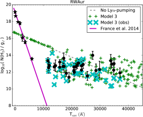
Figure 13: The rotation diagram for RW Aur, with rovibrational column densities derived in this study (black circles) and lower energy states calculated by France et al. (2014a) (black stars; $\lambda\lambda$ 1092.5 $-$ 1117 Å). The magenta solid line shows the thermal distribution H₂ levels examined by France et al. (2014a), with log₁₀( N(H₂) ) $=$ 19.90 cm^-2 and T(H₂) $=$ 440 K. The green plus symbols represent the H₂ rovibrational levels output by the Ly$\alpha$-pumping models (Model 3). The cyan “X”s mark rovibrational levels from Model 3 which match the observed $H_{2}$ levels, so the reader can directly compare the the data with the modeled states. The gray dashed line presents the initial thermal distribution of H₂ in the models (i.e., without Ly$\alpha$ pumping), which is described by log₁₀( N(H₂) ) $=$ 18.03 and T(H₂) = 2504 K.

One of the first things we notice about the Model 3 results is that the H₂ rovibrational levels are redistributed in such a way that more highly excited H₂ levels ($T_{exc}$ $\gtrsim$ 30,000 K) can be pumped to higher column densities than they are expected to be in thermal distributions. Rovibrational levels of H₂ most affected by the flux of Ly$\alpha$ (i.e., $v$ $\geq$ 2; $T_{exc}$ $\sim$ 10,000 K) first appear diminished in column density, relative to the native thermal distributions, but for rovibrational levels with $T_{exc}$ $\gtrsim$ 30,000 K, the relative column densities of highly energetic states appears to return back towards the level of the thermal distribution, with many states being pumped by $\gtrsim$ 1 dex more than they would otherwise be in thermally-distributed states.

Additionally, the re-distributed H₂ rovibrational levels appear scattered, with the behavior of the scattered distributions appearing roughly consistent for rovibrational levels with $T_{exc}$ $\gtrsim$ 10,000 K and with a spread of $\sim$1 dex. We note that this behavior matches the characteristic distributions of empirically-derived H₂ rovibration levels measured against Ly$\alpha$ for most, if not all, of our PPD sightlines. The Ly$\alpha$ redistribution appears to scatter most H₂ states out of thermal equilibrium at T_exc $\gtrsim$ 10,000 K, suggesting that the H₂ absorption coincident on the Ly$\alpha$ wings do not probe thermal populations of H₂ in these sightlines. The fact that we see this same peculiar H₂ population behavior for all disks in our survey, regardless of orientation of the disk in the line of sight (i.e., i_disk), suggests that the sampling of H₂ may not be co-spatial with the same H₂ populations observed in fluorescence from each disk. The models also suggest that, for rovibrational levels insensitive to Ly$\alpha$ radiation (i.e., $v$ $<$ 2), H₂ may still be thermally populated. Theoretically, if we could observe rovibrational levels of H₂ not pumped by Ly$\alpha$ radiation, we could test this hypothesis.

We do have one case study - RW Aur - where this test is currently possible. The sightline to RW Aur probes both hot H₂ embedded in the Ly$\alpha$ profile of the protostar and warm H₂ in the FUV continuum ($\lambda\lambda$ 1090 - 1120 Å; France et al. 2014b). If the warm disk H₂ populations and the hot Ly$\alpha$ H₂ populations were co-spatial with one another, we would expect to find signatures in the FUV-continuum probing the same hot H₂ population (specifically for $v$ = 0, $J$ = 4, 5, 6; $\lambda$ = 1100.2, 1104.1, 1104.5, 1109.3, 1109.9, 1115.5, 1116.0 Å, where the distributions of warm and hot H₂ populations overlap). From the Ly$\alpha$-pumping model results for RW Aur, we expect to find appreciable thermal columns of hot H₂ in the sightline, which is several dex denser than the warm H₂ probed by the FUV continuum. The FUV continuum is much less likely to scatter through the gas disk than Ly$\alpha$, and therefore is expected to provide a better probe of the geometry through the disk material. The fact that the France et al. (2014b) study does not see clear deviations to the larger column density found by Model 3 for hot H₂[$v$ = 0, $J$ = 4, 5, 6] in the FUV continuum is further evidence supporting our original hypothesis - that the resonance nature of Ly$\alpha$ allows the radiation to scatter through a hot atomic halo above the PPD, and the observed H₂ signatures observed in the protostellar Ly$\alpha$ wings probe residual H₂ in these environments, rather than in the disk.

6 Conclusions

We perform the first empirical survey of H₂ absorption observed against the stellar Ly$\alpha$ emission profiles of 22 PPD hosts. The aim of this study was to identify thermal and non-thermal H₂ species in each sightline and investigate excitation mechanisms responsible for the distributions of non-thermal H₂ populations. We normalize each Ly$\alpha$ profile and create optical depth models to synthesize H₂ absorption features observed across the normalized Ly$\alpha$ spectra. Each optical depth model estimates the column density of H₂ in ground states [$v$,$J$] from the absorption depth in the Ly$\alpha$ wings, and we present the H₂ rotation diagrams of all samples in our survey to examine the behavior of the H₂ rovibrational populations in all sightlines. Below, we highlight our findings and conclusions:

• Thermally-distributed H₂ models alone cannot reproduce observed rovibration levels. Highly-energetic states are “pumped” when compared with lower energy rovibrational states. This appears to happen at “knee” junctures, which are consistently found at T_exc = 20,000 K, 25,000-26,000 K, and 31,000-32,000 K.

• We find roughly-equivalent total column densities of thermal and non-thermal H₂ populations in transitional disk samples and samples with detectable C IV-pumped H₂ fluorescence. Primordial disk targets have more spread in this relation, and show more samples with larger total column densities of thermal H₂ than non-thermal H₂ populations.

• High energy continuum radiation, produced primarily by accretion processes onto the host protostar, appears to play an important role in regulating the total density of non-thermal H₂ in the circumstellar environment. We find correlations between the X-ray and FUV luminosities and N(H₂)${}_{\textnormal{nLTE}}$ and little evidence that line emission from protostellar accretion processes plays a significant role in regulating the total column densities of thermal and non-thermal H₂ states, except C IV, which appears to be anti-correlated with the total thermal column densities of H₂.

• There is a clear anti-correlation between N(H₂)${}_{\textnormal{nLTE}}$ and H₂ dissociation continuum, suggesting that photo-excitation may be more effective at unbinding H₂ already in highly energized levels than lower energy thermal states.

• From one target that has access to cooler H₂ populations observed against the FUV continuum (RW Aur A; France et al. 2014b), we see two populations of H₂: warm H₂ probing higher density material in the protoplanetary disk, and hot H₂ in an atomic halo surrounding the protostar and disk. The total column of warm H₂ is several dex higher than the total column of hot H₂ in the Ly$\alpha$ wings. We see a crossing point, where we should begin to see warmer columns of H₂ in the FUV continuum (T_exc $\approx$ 3,000 K), but, observationally, this does not appear to be the case. H I-Ly$\alpha$ is a strong resonance , and a small amount of residual H I in the protostellar environment will scatter Ly$\alpha$ before it escapes. We suspect that the H₂ populations probed in the protostellar Ly$\alpha$ wings are not associated with the disk, but rather found in a tenuous halo of hot, mostly atomic gas around the disk. The hot H₂ also probes much lower column densities ($\langle$N(H₂)$\rangle$ $\sim$ 10¹⁶ cm^-2) of H₂ than is required to produce the observe fluorescence in these same PPD samples, strongly suggesting that absorption and fluorescence H₂ populations are not co-spatial.

While this study examined the behavior of hot H₂ in protoplanetary disk environments, further investigation and proper implementation of non-LTE models is necessary to pinpoint the physics driving H₂ to higher [$v$,$J$] states. Studies have been performed that point to several mechanisms driving H₂ populations, including collisions with other particles and higher energy photons (FUV/EUV/X-ray; Nomura et al. (2005); Nomura & Millar (2005); Ádámkovics et al. (2016)) and reformation/destruction of H₂ by chemical evolution, especially H₂O dissociation in the warm disk atmosphere (Du & Bergin, 2014; Glassgold & Najita, 2015). The next step forward would be to implement radiative, collisional, and chemical processes simultaneously to simulate the PPD environmental behavior. Paper II will address the spatial origins of this H₂ absorption, based on results from this study and empirical evidence from the absorption features themselves.

Appendix A Additional Details on H₂ Absorption Line Analysis

Fig. Set1. The Ly$\alpha$ profiles of each PPD host

Information about each H₂ absorption transition was found either in Abgrall et al. (1993a) or Abgrall et al. (1993b), specifically the Einstein A-coefficient, describing the rate of spontaneous decay from state $u$ $\rightarrow$ $l$ ($A_{ul}$), and the wavenumber. All H₂ transitions were selected from Roncin & Launay (1995) between 1210 - 1221 Å, with transitions preferentially considered from those previously called out by Herczeg et al. (2002) and France et al. (2012a). Other H₂ transitions included in the line-fitting analysis met a minimum (A_ul) $\geq$ 3.0$\times$10⁷ s^-1, to ensure that the absorption transition probabilities were large enough for detection, assuming a warm thermal population of H₂. The energy levels of ground state H₂ in vibration and rotation levels [$v$,$J$] (E_gr) were derived from equations outlined in H₂ools (McCandliss, 2003), with physical constants taken from Herzberg (1950), Jennings et al. (1984), and Draine (2011). The physical properties of the H₂ transition were derived from intrinsic properties of the molecule:

$$\sigma(\lambda)=\left(\frac{\lambda_{\lambda}^{3}}{8\pi c}\right)\left(\frac{g_{u}}{g_{l}}\right)A_{ul}$$ (A1)

$$f_{lu}=\left(\frac{m_{e}c}{8\pi^{2}e^{2}}\right)\left(\frac{g_{u}}{g_{l}}\right)\lambda_{lu}^{2}A_{ul}$$ (A2)

where $\lambda_{\lambda}$ is the photo-excitation wavelength, Ly$\alpha$, of H₂ in ground state [$v$,$J$]; $g_{u}$ and $g_{l}$ are the statistical weights of the electronically-excited [$v^{\prime}$,$J^{\prime}$] and ground [$v$,$J$] states, respectively; and ($\pi e^{2}/m_{e}c$) is the definition of the classical cross section, expressed as 0.6670 cm² s^-1 in cgs units. Table 2 shows all transitions used in our H₂ synthetic absorption model, including physical properties (E_gr, $f_{lu}$, $A_{ul}$) and level transition information. Not all transitions were implemented for every target. Depending on the effective range of the stellar Ly$\alpha$ wing in wavelength space, many of the transitions found on the edges of the wings (1210 $-$ 1212: 1213.5 $-$ 1215.2 Å for the blue wing; 1216 $-$ 1218: 1219.5 $-$ 1221 Å for the red wing) were omitted.

The modeled b-value is fixed in all synthetic absorption spectra to replicate the thermal width of a warm bulk population of H₂ (T(H₂) $\geq$ 2500 K) in the absence of turbulent velocity broadening. If the b-value were larger, the broadening acts to widen the absorption feature and diminish the depth of the line center, which causes degeneracy between the estimated rovibrational [$v$,$J$] level column densities and the thermal/turbulent parameters of the models. When we increased $b_{H_{2}}$ $=$ 10 km s^-1, the column densities of the rovibrational [$v$,$J$] levels were systematically reduced by 0.1-0.7 dex for all survey samples.

The multi-component fit of H₂ absorption was mostly insensitive to initial conditions. Initially, we set the same initial conditions for the start of the run ($v_{r}$ = 0 km s^-1; T(H₂) = 2500 K; log₁₀ N(H₂;$v$,$J$) varied by transition properties) and allowed the parameters float. Once an effective range of values was determined for all targets, T(H₂) and $b_{H_{2}}$ were fixed, and only $v_{r}$ was allowed to float. This produces column density estimates that are relatively comparable for all targets in our survey.

As discussed in France et al. (2012a), only the (0-2)R(2) and (2-2)P(9) levels, whose wavelengths differed by $\Delta\lambda$ = 0.01 Å (at 1219.09 and 1219.10 Å, respectively), were sensitive to the initial conditions. The total column density at this wavelength range is robust, while the relative columns shared between the two transitions was not. To mitigate this, we weighed the individual columns by the product of their oscillator strengths and relative populations of the two levels at T(H₂) = 2500 K. Using the methodology laid out in H₂ools and Equation A2, we calculate the oscillator strengths and relative populations of the two lines to be [$f_{R(2)}$ = 25.5 $\times$ 10^-3; $P_{R(2)}$ = 5.76 $\times$ 10^-4] and [$f_{R(9)}$ = 31.8 $\times$ 10^-3; $P_{R(9)}$ = 6.24 $\times$ 10^-4], respectively. Therefore, N(2,2) contributes 0.425 of the total column density determined at 1219.10 Å, while N(2,9) contributes 0.575 of the total column. Column 2 of Figure 2 show the minimized multi-component synthetic spectra plotted over the normalized Ly$\alpha$ wings for the red-ward and blue-ward profile components, respectively.

Fig. Set2. The Relative Absorption Spectra and H₂ Optical Depth Models of each PPD host Ly$\alpha$ emission wing.

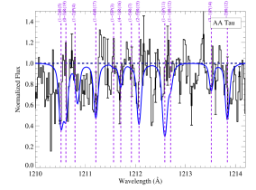
(a)

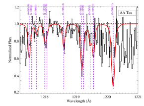
(b)

Figure 2: The final, synthesized absorption spectra of warm H₂ against the Ly$\alpha$ transmission spectra. For targets that have transmission spectra for both blue and red Ly$\alpha$ wings, blue wing spectra are shown on the left (blue H₂ absorption fit) and red wing spectra are on the right (red H₂ absorption fit). For targets with only a red-wing transmission spectrum, red-wing fits are shown on the left (red H₂ absorption fit).

Appendix B H₂ Model Details and Monte Carlo Simulations

B.1 Models 1 & 2: Thermal H₂ Populations only

Models 1 and 2 are simple models that follow the H₂ools layout: Given the derived column densities for observed H₂ ground states against the stellar Ly$\alpha$ wing N(H₂;$v$,$J$), we use first principles molecular physics to determine the theoretical population column densities of a bulk H₂ population N(H₂) described by a shared thermal profile T(H₂). The level column densities are calculated using Boltzmann populations, assuming LTE conditions, and each ground state energy level is determined by calculating the electronic, vibrational, and rotational energy levels for a ground state [$v$,$J$], as described in McCandliss (2003).

Model 1 assumes that all data points extracted from the absorption features of each target are thermally-populated. Model 2 assumes only H₂ populations with ground state energies E_gr $<$ 1.5 eV (T_exc $\lesssim$ 17500 K) are thermally-populated, with the possibility that H₂ in ground states with E_gr $>$ 1.5 eV are pumped additionally by some unknown non-thermal process(es), and so are not considered in the model-data comparison. We use Model 2 as a baseline of the minimum N(H₂) and T(H₂) of thermal H₂ in the disk atmosphere for each target, assuming any of the observed, absorbing H₂ against the Ly$\alpha$ wing is purely thermally excited.

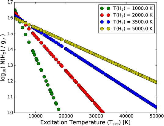
Figure 16: Modeled rotation diagram of H₂ populations found in thermal equilibrium with a set N(H₂) = 10¹⁷ cm^-2 and varying thermal descriptions T(H₂). As T(H₂) increases, more H₂ populations with higher excitation temperatures, T_exc, become populated, increasing the relative ratio of higher T_exc state to lower T_exc states, which decreases the slope of the distribution towards zero. This model is used to compare the observed rotation profiles of H₂ to thermally-populated states of H₂ for Models 1 and 2.

Figure 16 shows an example of how the relative [$v$,$J$] states are populated by the thermal distribution of H₂. While the total column density of H₂ regulates the column densities of H₂ found in ground state [$v$,$J$], T(H₂) determines the relative abundances of each [$v$,$J$] to others in the ground state. For example, a lower T(H₂) means that, statistically, more H₂ is found in ground states with low [$v$,$J$] because the overall excess energy in the H₂ populations is low. However, as T(H₂) increases, the ratio of the abundances of H₂ found in higher [$v$,$J$] states to those in low [$v$,$J$] states increases. This appears as a “flattening” of the slope of H₂ populations in Figure 16.

Fig. Set3. Fitting Thermal Models to Each H₂ Rotation Diagram

Appendix C MCMC Simulations

Each model is compared to the resulting rotation diagrams derived from the relative H₂ absorption column densities derived as explained in Section 3. This is done using a MCMC routine, which randomly-generates initial parameter conditions and minimizes the likelihood function ($\ln\operatorname{\mathcal{L}}$(x,$\theta$)) between the H₂ rovibration column densities and model parameters. We define $\ln\operatorname{\mathcal{L}}$(x,$\theta$) as a $\chi^{2}$ statistic, with an additional term to explore the weight of standard deviations on each rovibrational column density:

$$\ln\operatorname{\mathcal{L}}(\textnormal{x},\theta,f)=\frac{(y(\textnormal{x})-y(\textnormal{x},\theta))^{2}}{\sigma^{2}}-\ln((\sigma^{2}+y(\textnormal{x},\theta)^{2}\exp(2f))^{-1})$$ (C1)

In Equation C1, x represents the ground state energy of H₂ in rovibration level [$v$,$J$], $y$(x) is the observed column density of H₂, $y$(x,$\theta$) is the modeled column density of H₂ derived from the thermal model, $\sigma^{2}$ is the variance in the column densities, and $f$ is an estimation on the accuracy of the column density standard deviations. For parameters shared between all thermal model runs (N(H₂), T(H₂), $\ln f$), we set prior information about each to keep the model outputs physically viable. We let the total thermal H₂ column density range from N(H₂) = 12.0 $-$ 25.0 cm^-2. Below N(H₂) = 12.0 cm^-2, there is not enough column in individual rovibrational levels to produce measurable absorption features in the data. Additionally, N(H₂) $\geq$ 25.0 cm^-2 will significantly saturate the features in the absorption spectra, which we do not see for any target in our survey. The thermal populations of H₂ are allowed to range from T(H₂) = 100 $-$ 5000 K. The H₂ populations must be warm enough to populate the correct rovibrational levels that absorb Ly$\alpha$ photons, while simultaneously cooler than the dissociation temperature of H₂ (T(H₂)_diss $\approx$ 5000 K).

For Models 1 and 2, MCMC simulations were run with 300 independent initial randomly-generated parameter realizations (walkers) and allowed to vary over 1000 steps to converge on the best representation of the observations.

C.1 Model 3: Thermal H₂ Populations Photo-excited by HI-Ly$\alpha$

Model 3 uses the same thermal populations of Models 1 and 2 and adds an additional photo-pumping mechanism to show how thermal populations reach an equilibrium state in the presence of an external radiation field. First, because we observe H₂ absorption against the Ly$\alpha$ wings of these targets and Ly$\alpha$ radiation makes up the vast majority of the FUV radiation that photo-excited H₂ to fluorescence, we assume the radiation pumping the thermal states to new equilibrium populations is dominated by Ly$\alpha$. To describe the amount of radiation being absorbed by H₂, we add two additional parameters that describe the flux input to the system, $F_{n}(\lambda)$ and $F_{b}(\lambda)$, which represent a narrow and broad flux component from the stellar Ly$\alpha$ radiation incident on the H₂ populations. Following the results and analysis from McJunkin et al. (2014), we assume the Ly$\alpha$ radiation profile incident with the H₂ on the disk surface is described by two Gaussian components - a narrow component, where the bilk of the flux is located, and a broad component, which describes the shape of the observed outer wings. McJunkin et al. (2014) find full width at half maximum (FWHM) fits for both the narrow and broad Gaussian components of the radiation distribution, and we use those results to describe the width of our input flux. We allow the peak fluxes of both the narrow and broad flux distributions to vary and have final input Ly$\alpha$ flux distributions described by:

$$\begin{split}F_{\textnormal{Ly}\alpha}(\lambda)&=F_{n}\left(\lambda\right)+F_{b}\left(\lambda\right)\\ &=F_{n}\exp\left(\frac{-\Delta\lambda^{2}}{2\sigma_{n}^{2}}\right)+F_{b}\exp\left(\frac{-\Delta\lambda^{2}}{2\sigma_{b}^{2}}\right),\end{split}$$ (C2)

where $F_{n}$ and $F_{b}$ are free parameters in the models, and $\sigma_{n}$ and $\sigma_{b}$ are derived from the FWHM found in McJunkin et al. (2014), and $\Delta\lambda$ = $\lambda-\lambda_{lab}$, where $\lambda_{lab}$ is the rest wavelength of HI-Ly$\alpha$ (1215.67 Å). Each flux distribution is kept constant throughout the model run, assuming the output radiation from the star over the time it takes to equalize the photo-pumped populations of H₂ is isotropic. We assume $F_{n}(\lambda)$ and $F_{b}(\lambda)$ are observed flux rates, and we therefore infer the flux back to the star by reddening the flux with ISM extinction values determined by McJunkin et al. (2014). The allowed ranges of observed total Ly$\alpha$ flux are outlined in Schindhelm et al. (2012) for reconstructed Ly$\alpha$ profiles seen in at the PPDs. We constrain the Ly$\alpha$ flux to log₁₀($F_{n}(\lambda)$) = -13 to -5 ergs cm^-2 s^-1 and log₁₀($F_{b}(\lambda)$) = -16 to -5 ergs cm^-2 s^-1, which are integrated over each Gaussian function in Equation C2.

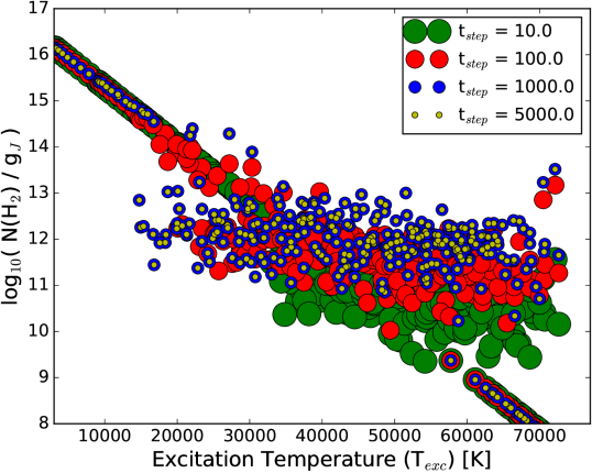
Figure 18: Modeled thermal distributions of H₂ with N(H₂) = 10¹⁷ cm^-2 and T(H₂) = 3500 K, assuming thermal populations of H₂ are constantly photo-excited by an external HI-Ly$\alpha$ radiation field to an equilibrium state. The Ly$\alpha$ radiation field is assumed to be Gaussian in shape when interacting with H₂ molecules, with a peak flux of 10^-9 ergs cm^-2 s^-1 at 1215.67 Å. We show how the number of iterations of time the H₂ is exposed to the Ly$\alpha$ flux affects the distribution of H₂ ground states. We find that iterations t_step = 1000 reaches a final equilibrium state. The thermal distribution + Ly$\alpha$ pumping mechanics are used to calculate theoretical H₂ populations in Model 3.

Once flux and thermal H₂ population parameters are chosen, we follow the change in thermal populations in states [$v$,$J$] of H₂ being exposed to the pumping radiation in time iterations of the pumping process, t_step, where each t_step is considered over some arbitrary $\Delta$t. First, we find how much H₂ in state [$v$,$J$] is lost to be pumped to some electronic excited state [$v^{\prime}$,$J^{\prime}$] because of the interaction with a discrete Ly$\alpha$ photon with wavelength $\lambda$. We determine how much H₂ is photo-excited by $\lambda$ by calculating the cross section for absorption of photon $\lambda$, given the transition probabilities of the H₂ rovibration levels. Once all [$v$,$J$] state losses via $\lambda$ absorption have been determined, we allow the excited state H₂ to fluoresce back to the ground state via the branching ratios, or transition probabilities, to some final ground state [$v^{\prime\prime}$,$J^{\prime\prime}$].

For this simple model, we assume that dissociation of H₂ molecules by Ly$\alpha$-pumping is negligible. As Dalgarno & Stephens (1970) describe, nearly all Ly$\alpha$-pumped excited states have bound de-exciation levels, such that transitions from the Lyman band are expected to have very low probabilities of dissociation. While there exist a handful of Werner-band transitions, which likely prose the greatest probability for molecular dissociation upon decay, this simple model does not contain a source term of H₂, such that we cannot control the formation of H₂ at any point in the model. To keep the modeled distributions of H₂ constant throughout the simulated experiment, therefore, we assume that all H₂ transitions result only in the decay of H₂ to arbitrary ground states, with no probability that H₂ dissociates via these fluorescence routes.

This process is repeated until the H₂ populations reach a steady-state equilibrium, such that the absorption out of state [$v$,$J$] equalizes with the cascade back to [$v^{\prime\prime}$,$J^{\prime\prime}$]. For T(H₂) $\leq$ 5000 K, this equilibrium is reached by t_step = 1000. With higher N(H₂), we find that it takes more t_step to reach equilibrium, but for N(H₂) $<$ 10²⁰ cm^-2 and high T(H₂), an equilibrium state is reached after t_step $\approx$ 3000 steps. Figure 18 shows how the distributions of thermal H₂ populations change when exposed to a constant Ly$\alpha$ flux from the host star, as a function of time steps from first exposure. If we assume the distributions of H₂ ground states are primarily affected by photo-pumping via Ly$\alpha$ photons and no other physical mechanisms to drive the populations to non-LTE states (collisions with other species, chemical evolution, etc), then equilibrium of H₂ states is reached fairly quickly and does not change from the final equilibrium state of populations.

We perform the same MCMC data-model reduction for Model 3 and the observed rotation diagrams. Model 3 required time iterations and, therefore, took longer to run. We ran two separate iteration of Model 3, the first MCMC simulation having 100 independent walkers varying over the parameter space iterating over 2000 steps with 1000 time iterations of the Ly$\alpha$-pumping. We determined that, after about 100 converging steps for each walker, we were able to settle into the best realization of the data. We also determined that longer time iterations were necessary to settle the Ly$\alpha$-pumping mechanism into equilibrium for larger column densities (N(H₂) $>$ 10²⁰ cm^-2) and temperatures (T(H₂) $>$ 4500 K). We ran a second iteration of MCMC simulations for Model 3 using t_step = 5000 per model realization, with 100 independent MCMC walkers iterating over 500 steps to convergence. Because of the extensive computation time of Model 3 with 5000 time steps per model realization, we chose to cut the total number of convergence steps to keep the same number of walker realizations in the MCMC.

Table 4 presents parameter results for all modeled H₂ thermal distributions. For all Model 3 realizations, $F_{b}(\lambda)$ has been excluded, since the majority of the integrated flux of Ly$\alpha$ is dominated by $F_{n}(\lambda)$ ($F_{n}(\lambda)$ $>>$ $F_{b}(\lambda)$). Figure LABEL:app:fig5 shows the best-fit, median model parameters for Model 3 with observed rovibration H₂ levels overplotted. We mark each modeled rovibration level with a green plus symbol, and we mark modeled rovibration levels which are probed in the observed Ly$\alpha$ wing(s) of the target with cyan crosses.

Fig. Set4. Fitting Ly$\alpha$-Pumping Models to Each H₂ Rotation Diagram

References

- Abgrall et al. (1993a) Abgrall, H., Roueff, E., Launay, F., Roncin, J. Y., & Subtil, J. L. 1993a, A&AS, 101, 273
- Abgrall et al. (1993b) —. 1993b, A&AS, 101, 323
- Ádámkovics et al. (2016) Ádámkovics, M., Najita, J. R., & Glassgold, A. E. 2016, ApJ, 817, 82
- Aikawa & Nomura (2006) Aikawa, Y. & Nomura, H. 2006, ApJ, 642, 1152
- Akeson et al. (2002) Akeson, R. L., Ciardi, D. R., van Belle, G. T., & Creech-Eakman, M. J. 2002, ApJ, 566, 1124
- Alencar et al. (2003) Alencar, S. H. P., Melo, C. H. F., Dullemond, C. P., Andersen, J., Batalha, C., Vaz, L. P. R., & Mathieu, R. D. 2003, A&A, 409, 1037
- Alexander et al. (2014) Alexander, R., Pascucci, I., Andrews, S., Armitage, P., & Cieza, L. 2014, Protostars and Planets VI, 475
- Alexander & Armitage (2007) Alexander, R. D. & Armitage, P. J. 2007, MNRAS, 375, 500
- Alexander et al. (2006) Alexander, R. D., Clarke, C. J., & Pringle, J. E. 2006, MNRAS, 369, 229
- Andrews & Williams (2007) Andrews, S. M. & Williams, J. P. 2007, ApJ, 671, 1800
- Andrews et al. (2011) Andrews, S. M., Wilner, D. J., Espaillat, C., Hughes, A. M., Dullemond, C. P., McClure, M. K., Qi, C., & Brown, J. M. 2011, ApJ, 732, 42
- Ardila et al. (2002) Ardila, D. R., Basri, G., Walter, F. M., Valenti, J. A., & Johns-Krull, C. M. 2002, ApJ, 566, 1100
- Ardila et al. (2013) Ardila, D. R., Herczeg, G. J., Gregory, S. G., Ingleby, L., France, K., Brown, A., Edwards, S., Johns-Krull, C., Linsky, J. L., Yang, H., Valenti, J. A., Abgrall, H., Alexander, R. D., Bergin, E., Bethell, T., Brown, J. M., Calvet, N., Espaillat, C., Hillenbrand, L. A., Hussain, G., Roueff, E., Schindhelm, E. R., & Walter, F. M. 2013, ApJS, 207, 1
- Armitage et al. (2003) Armitage, P. J., Clarke, C. J., & Palla, F. 2003, MNRAS, 342, 1139
- Arulanantham et al. (2016) Arulanantham, N. A., Herbst, W., Gilmore, M. S., Cauley, P. W., & Leggett, S. K. 2016, ArXiv e-prints
- Ayliffe & Bate (2010) Ayliffe, B. A. & Bate, M. R. 2010, MNRAS, 408, 876
- Ayres (2010) Ayres, T. R. 2010, VizieR Online Data Catalog, 218
- Bai (2016) Bai, X.-N. 2016, ApJ, 821, 80
- Banzatti & Pontoppidan (2015) Banzatti, A. & Pontoppidan, K. M. 2015, ApJ, 809, 167
- Bary et al. (2003) Bary, J. S., Weintraub, D. A., & Kastner, J. H. 2003, ApJ, 586, 1136
- Beck et al. (2012) Beck, T. L., Bary, J. S., Dutrey, A., Piétu, V., Guilloteau, S., Lubow, S. H., & Simon, M. 2012, ApJ, 754, 72
- Beckwith et al. (1983) Beckwith, S., Evans, II, N. J., Gatley, I., Gull, G., & Russell, R. W. 1983, ApJ, 264, 152
- Beckwith et al. (1978) Beckwith, S., Gatley, I., Matthews, K., & Neugebauer, G. 1978, ApJ, 223, L41
- Bergin et al. (2004) Bergin, E., Calvet, N., Sitko, M. L., Abgrall, H., D’Alessio, P., Herczeg, G. J., Roueff, E., Qi, C., Lynch, D. K., Russell, R. W., Brafford, S. M., & Perry, R. B. 2004, ApJ, 614, L133
- Bertout et al. (1988) Bertout, C., Basri, G., & Bouvier, J. 1988, ApJ, 330, 350
- Bertout et al. (1999) Bertout, C., Robichon, N., & Arenou, F. 1999, A&A, 352, 574
- Bethell & Bergin (2011) Bethell, T. J. & Bergin, E. A. 2011, ApJ, 739, 78
- Black & Dalgarno (1977) Black, J. H. & Dalgarno, A. 1977, ApJS, 34, 405
- Böhm et al. (2004) Böhm, T., Catala, C., Balona, L., & Carter, B. 2004, A&A, 427, 907
- Bouvier et al. (1999) Bouvier, J., Chelli, A., Allain, S., Carrasco, L., Costero, R., Cruz-Gonzalez, I., Dougados, C., Fernández, M., Martín, E. L., Ménard, F., Mennessier, C., Mujica, R., Recillas, E., Salas, L., Schmidt, G., & Wichmann, R. 1999, A&A, 349, 619
- Brown et al. (2009) Brown, J. M., Blake, G. A., Qi, C., Dullemond, C. P., Wilner, D. J., & Williams, J. P. 2009, ApJ, 704, 496
- Brown et al. (2013) Brown, J. M., Pontoppidan, K. M., van Dishoeck, E. F., Herczeg, G. J., Blake, G. A., & Smette, A. 2013, ApJ, 770, 94
- Calvet et al. (2002) Calvet, N., D’Alessio, P., Hartmann, L., Wilner, D., Walsh, A., & Sitko, M. 2002, ApJ, 568, 1008
- Calvet et al. (2005) Calvet, N., D’Alessio, P., Watson, D. M., Franco-Hernández, R., Furlan, E., Green, J., Sutter, P. M., Forrest, W. J., Hartmann, L., Uchida, K. I., Keller, L. D., Sargent, B., Najita, J., Herter, T. L., Barry, D. J., & Hall, P. 2005, ApJ, 630, L185
- Cartwright & Drapatz (1970) Cartwright, D. C. & Drapatz, S. 1970, A&A, 4, 443
- Coffey et al. (2004) Coffey, D., Bacciotti, F., Woitas, J., Ray, T. P., & Eislöffel, J. 2004, ApJ, 604, 758
- Comerón & Fernández (2010) Comerón, F. & Fernández, M. 2010, A&A, 511, A10
- Comerón et al. (2003) Comerón, F., Fernández, M., Baraffe, I., Neuhäuser, R., & Kaas, A. A. 2003, A&A, 406, 1001
- Correia et al. (2006) Correia, S., Zinnecker, H., Ratzka, T., & Sterzik, M. F. 2006, A&A, 459, 909
- Dalgarno & Stephens (1970) Dalgarno, A. & Stephens, T. L. 1970, ApJ, 160, L107
- Danforth et al. (2010) Danforth, C. W., Stocke, J. T., & Shull, J. M. 2010, ApJ, 710, 613
- Dodson-Robinson & Salyk (2011) Dodson-Robinson, S. E. & Salyk, C. 2011, ApJ, 738, 131
- Donehew & Brittain (2011) Donehew, B. & Brittain, S. 2011, AJ, 141, 46
- Dong et al. (2015) Dong, R., Zhu, Z., & Whitney, B. 2015, ApJ, 809, 93
- Draine (2011) Draine, B. T. 2011, Physics of the Interstellar and Intergalactic Medium
- Draine & Bertoldi (1996) Draine, B. T. & Bertoldi, F. 1996, ApJ, 468, 269
- Du & Bergin (2014) Du, F. & Bergin, E. A. 2014, ApJ, 792, 2
- Dullemond et al. (2007) Dullemond, C. P., Hollenbach, D., Kamp, I., & D’Alessio, P. 2007, Protostars and Planets V, 555
- Dullemond & Monnier (2010) Dullemond, C. P. & Monnier, J. D. 2010, ARA&A, 48, 205
- Eisner et al. (2007) Eisner, J. A., Hillenbrand, L. A., White, R. J., Bloom, J. S., Akeson, R. L., & Blake, C. H. 2007, ApJ, 669, 1072
- Espaillat et al. (2007) Espaillat, C., Calvet, N., D’Alessio, P., Bergin, E., Hartmann, L., Watson, D., Furlan, E., Najita, J., Forrest, W., McClure, M., Sargent, B., Bohac, C., & Harrold, S. T. 2007, ApJ, 664, L111
- Espaillat et al. (2011) Espaillat, C., Furlan, E., D’Alessio, P., Sargent, B., Nagel, E., Calvet, N., Watson, D. M., & Muzerolle, J. 2011, ApJ, 728, 49
- Fedele et al. (2010) Fedele, D., van den Ancker, M. E., Henning, T., Jayawardhana, R., & Oliveira, J. M. 2010, A&A, 510, A72
- Feigelson et al. (2003) Feigelson, E. D., Lawson, W. A., & Garmire, G. P. 2003, ApJ, 599, 1207
- Ferreira et al. (2006) Ferreira, J., Dougados, C., & Cabrit, S. 2006, A&A, 453, 785
- Fleming et al. (2010) Fleming, B., France, K., Lupu, R. E., & McCandliss, S. R. 2010, ApJ, 725, 159
- Foreman-Mackey et al. (2013) Foreman-Mackey, D., Hogg, D. W., Lang, D., & Goodman, J. 2013, PASP, 125, 306
- France et al. (2012a) France, K., Burgh, E. B., Herczeg, G. J., Schindhelm, E., Yang, H., Abgrall, H., Roueff, E., Brown, A., Brown, J. M., & Linsky, J. L. 2012a, ApJ, 744, 22
- France et al. (2014a) France, K., Herczeg, G. J., McJunkin, M., & Penton, S. V. 2014a, ApJ, 794, 160
- France et al. (2017) France, K., Roueff, E., & Abgrall, H. 2017, ApJ, In Preparation
- France et al. (2014b) France, K., Schindhelm, E., Bergin, E. A., Roueff, E., & Abgrall, H. 2014b, ApJ, 784, 127
- France et al. (2011) France, K., Schindhelm, E., Burgh, E. B., Herczeg, G. J., Harper, G. M., Brown, A., Green, J. C., Linsky, J. L., Yang, H., Abgrall, H., Ardila, D. R., Bergin, E., Bethell, T., Brown, J. M., Calvet, N., Espaillat, C., Gregory, S. G., Hillenbrand, L. A., Hussain, G., Ingleby, L., Johns-Krull, C. M., Roueff, E., Valenti, J. A., & Walter, F. M. 2011, ApJ, 734, 31
- France et al. (2012b) France, K., Schindhelm, E., Herczeg, G. J., Brown, A., Abgrall, H., Alexander, R. D., Bergin, E. A., Brown, J. M., Linsky, J. L., Roueff, E., & Yang, H. 2012b, ApJ, 756, 171
- Frisch et al. (1999) Frisch, P. C., Dorschner, J. M., Geiss, J., Greenberg, J. M., Grün, E., Landgraf, M., Hoppe, P., Jones, A. P., Krätschmer, W., Linde, T. J., Morfill, G. E., Reach, W., Slavin, J. D., Svestka, J., Witt, A. N., & Zank, G. P. 1999, ApJ, 525, 492
- Furlan et al. (2009) Furlan, E., Watson, D. M., McClure, M. K., Manoj, P., Espaillat, C., D’Alessio, P., Calvet, N., Kim, K. H., Sargent, B. A., Forrest, W. J., & Hartmann, L. 2009, ApJ, 703, 1964
- Garcia Lopez et al. (2006) Garcia Lopez, R., Natta, A., Testi, L., & Habart, E. 2006, A&A, 459, 837
- Ghez et al. (1993) Ghez, A. M., Neugebauer, G., & Matthews, K. 1993, AJ, 106, 2005
- Glassgold et al. (2004) Glassgold, A. E., Najita, J., & Igea, J. 2004, ApJ, 615, 972
- Glassgold & Najita (2001) Glassgold, A. E. & Najita, J. R. 2001, in Astronomical Society of the Pacific Conference Series, Vol. 244, Young Stars Near Earth: Progress and Prospects, ed. R. Jayawardhana & T. Greene, 251
- Glassgold & Najita (2015) Glassgold, A. E. & Najita, J. R. 2015, ApJ, 810, 125
- Gómez de Castro (2009) Gómez de Castro, A. I. 2009, ApJ, 698, L108
- Gorti & Hollenbach (2004) Gorti, U. & Hollenbach, D. 2004, ApJ, 613, 424
- Gorti & Hollenbach (2009) —. 2009, ApJ, 690, 1539
- Gorti et al. (2015) Gorti, U., Hollenbach, D., & Dullemond, C. P. 2015, ApJ, 804, 29
- Grady et al. (2009) Grady, C. A., Schneider, G., Sitko, M. L., Williger, G. M., Hamaguchi, K., Brittain, S. D., Ablordeppey, K., Apai, D., Beerman, L., Carpenter, W. J., Collins, K. A., Fukagawa, M., Hammel, H. B., Henning, T., Hines, D., Kimes, R., Lynch, D. K., Ménard, F., Pearson, R., Russell, R. W., Silverstone, M., Smith, P. S., Troutman, M., Wilner, D., Woodgate, B., & Clampin, M. 2009, ApJ, 699, 1822
- Grady et al. (2004) Grady, C. A., Woodgate, B., Torres, C. A. O., Henning, T., Apai, D., Rodmann, J., Wang, H., Stecklum, B., Linz, H., Williger, G. M., Brown, A., Wilkinson, E., Harper, G. M., Herczeg, G. J., Danks, A., Vieira, G. L., Malumuth, E., Collins, N. R., & Hill, R. S. 2004, ApJ, 608, 809
- Green et al. (2012) Green, J. C., Froning, C. S., Osterman, S., Ebbets, D., Heap, S. H., Leitherer, C., Linsky, J. L., Savage, B. D., Sembach, K., Shull, J. M., Siegmund, O. H. W., Snow, T. P., Spencer, J., Stern, S. A., Stocke, J., Welsh, B., Béland, S., Burgh, E. B., Danforth, C., France, K., Keeney, B., McPhate, J., Penton, S. V., Andrews, J., Brownsberger, K., Morse, J., & Wilkinson, E. 2012, ApJ, 744, 60
- Güdel et al. (2007) Güdel, M., Skinner, S. L., Mel’Nikov, S. Y., Audard, M., Telleschi, A., & Briggs, K. R. 2007, A&A, 468, 529
- Gullbring et al. (2000) Gullbring, E., Calvet, N., Muzerolle, J., & Hartmann, L. 2000, ApJ, 544, 927
- Gullbring et al. (1998) Gullbring, E., Hartmann, L., Briceño, C., & Calvet, N. 1998, ApJ, 492, 323
- Habart et al. (2004) Habart, E., Boulanger, F., Verstraete, L., Walmsley, C. M., & Pineau des Forêts, G. 2004, A&A, 414, 531
- Hartigan et al. (1995) Hartigan, P., Edwards, S., & Ghandour, L. 1995, ApJ, 452, 736
- Hartmann et al. (1998) Hartmann, L., Calvet, N., Gullbring, E., & D’Alessio, P. 1998, ApJ, 495, 385
- Hashimoto et al. (2011) Hashimoto, J., Tamura, M., Muto, T., Kudo, T., Fukagawa, M., Fukue, T., Goto, M., Grady, C. A., Henning, T., Hodapp, K., Honda, M., Inutsuka, S., Kokubo, E., Knapp, G., McElwain, M. W., Momose, M., Ohashi, N., Okamoto, Y. K., Takami, M., Turner, E. L., Wisniewski, J., Janson, M., Abe, L., Brandner, W., Carson, J., Egner, S., Feldt, M., Golota, T., Guyon, O., Hayano, Y., Hayashi, M., Hayashi, S., Ishii, M., Kandori, R., Kusakabe, N., Matsuo, T., Mayama, S., Miyama, S., Morino, J.-I., Moro-Martin, A., Nishimura, T., Pyo, T.-S., Suto, H., Suzuki, R., Takato, N., Terada, H., Thalmann, C., Tomono, D., Watanabe, M., Yamada, T., Takami, H., & Usuda, T. 2011, ApJ, 729, L17
- Herczeg & Hillenbrand (2008) Herczeg, G. J. & Hillenbrand, L. A. 2008, ApJ, 681, 594
- Herczeg et al. (2002) Herczeg, G. J., Linsky, J. L., Valenti, J. A., Johns-Krull, C. M., & Wood, B. E. 2002, ApJ, 572, 310
- Herczeg et al. (2006) Herczeg, G. J., Linsky, J. L., Walter, F. M., Gahm, G. F., & Johns-Krull, C. M. 2006, ApJS, 165, 256
- Herczeg et al. (2005) Herczeg, G. J., Walter, F. M., Linsky, J. L., Gahm, G. F., Ardila, D. R., Brown, A., Johns-Krull, C. M., Simon, M., & Valenti, J. A. 2005, AJ, 129, 2777
- Herczeg et al. (2004) Herczeg, G. J., Wood, B. E., Linsky, J. L., Valenti, J. A., & Johns-Krull, C. M. 2004, ApJ, 607, 369
- Hernández et al. (2007) Hernández, J., Calvet, N., Briceño, C., Hartmann, L., Vivas, A. K., Muzerolle, J., Downes, J., Allen, L., & Gutermuth, R. 2007, ApJ, 671, 1784
- Herzberg (1950) Herzberg, G. 1950, Molecular spectra and molecular structure. Vol.1: Spectra of diatomic molecules
- Hoadley et al. (2015) Hoadley, K., France, K., Alexander, R. D., McJunkin, M., & Schneider, P. C. 2015, ApJ, 812, 41
- Hollenbach & Tielens (1999) Hollenbach, D. J. & Tielens, A. G. G. M. 1999, Reviews of Modern Physics, 71, 173
- Hughes et al. (1994) Hughes, J., Hartigan, P., Krautter, J., & Kelemen, J. 1994, AJ, 108, 1071
- Ingleby et al. (2011) Ingleby, L., Calvet, N., Bergin, E., Herczeg, G., Brown, A., Alexander, R., Edwards, S., Espaillat, C., France, K., Gregory, S. G., Hillenbrand, L., Roueff, E., Valenti, J., Walter, F., Johns-Krull, C., Brown, J., Linsky, J., McClure, M., Ardila, D., Abgrall, H., Bethell, T., Hussain, G., & Yang, H. 2011, ApJ, 743, 105
- Jennings et al. (1984) Jennings, D. E., Bragg, S. L., & Brault, J. W. 1984, ApJ, 282, L85
- Johns-Krull & Valenti (2001) Johns-Krull, C. M. & Valenti, J. A. 2001, ApJ, 561, 1060
- Johns-Krull et al. (2000) Johns-Krull, C. M., Valenti, J. A., & Linsky, J. L. 2000, ApJ, 539, 815
- Kamp & Dullemond (2004) Kamp, I. & Dullemond, C. P. 2004, ApJ, 615, 991
- Kamp et al. (2005) Kamp, I., Dullemond, C. P., Hogerheijde, M., & Enriquez, J. E. 2005, in IAU Symposium, Vol. 231, Astrochemistry: Recent Successes and Current Challenges, ed. D. C. Lis, G. A. Blake, & E. Herbst, 377–386
- Kastner et al. (2016) Kastner, J. H., Principe, D. A., Punzi, K., Stelzer, B., Gorti, U., Pascucci, I., & Argiroffi, C. 2016, AJ, 152, 3
- Kimble et al. (1998) Kimble, R. A., Woodgate, B. E., Bowers, C. W., Kraemer, S. B., Kaiser, M. E., Gull, T. R., Heap, S. R., Danks, A. C., Boggess, A., Green, R. F., Hutchings, J. B., Jenkins, E. B., Joseph, C. L., Linsky, J. L., Maran, S. P., Moos, H. W., Roesler, F., Timothy, J. G., Weistrop, D. E., Grady, J. F., Loiacono, J. J., Brown, L. W., Brumfield, M. D., Content, D. A., Feinberg, L. D., Isaacs, M. N., Krebs, C. A., Krueger, V. L., Melcher, R. W., Rebar, F. J., Vitagliano, H. D., Yagelowich, J. J., Meyer, W. W., Hood, D. F., Argabright, V. S., Becker, S. I., Bottema, M., Breyer, R. R., Bybee, R. L., Christon, P. R., Delamere, A. W., Dorn, D. A., Downey, S., Driggers, P. A., Ebbets, D. C., Gallegos, J. S., Garner, H., Hetlinger, J. C., Lettieri, R. L., Ludtke, C. W., Michika, D., Nyquist, R., Rose, D. M., Stocker, R. B., Sullivan, J. F., Van Houten, C. N., Woodruff, R. A., Baum, S. A., Hartig, G. F., Balzano, V., Biagetti, C., Blades, J. C., Bohlin, R. C., Clampin, M., Doxsey, R., Ferguson, H. C., Goudfrooij, P., Hulbert, S. J., Kutina, R., McGrath, M., Lindler, D. J., Beck, T. L., Feggans, J. K., Plait, P. C., Sandoval, J. L., Hill, R. S., Collins, N. R., Cornett, R. H., Fowler, W. B., Hill, R. J., Landsman, W. B., Malumuth, E. M., Standley, C., Blouke, M., Grusczak, A., Reed, R., Robinson, R. D., Valenti, J. A., & Wolfe, T. 1998, ApJ, 492, L83
- Kraus & Hillenbrand (2009) Kraus, A. L. & Hillenbrand, L. A. 2009, ApJ, 704, 531
- Kriss (2011) Kriss, G. A. 2011, Improved Medium Resolution Line Spread Functions for COS FUV Spectra, Tech. rep.
- Lawson et al. (2001) Lawson, W. A., Crause, L. A., Mamajek, E. E., & Feigelson, E. D. 2001, MNRAS, 321, 57
- Lawson et al. (1996) Lawson, W. A., Feigelson, E. D., & Huenemoerder, D. P. 1996, MNRAS, 280, 1071
- Lawson et al. (2004) Lawson, W. A., Lyo, A.-R., & Muzerolle, J. 2004, MNRAS, 351, L39
- Levison et al. (2015) Levison, H. F., Kretke, K. A., & Duncan, M. J. 2015, Nature, 524, 322
- Lin & Papaloizou (1986) Lin, D. N. C. & Papaloizou, J. 1986, ApJ, 309, 846
- Loinard et al. (2007) Loinard, L., Torres, R. M., Mioduszewski, A. J., Rodríguez, L. F., González-Lópezlira, R. A., Lachaume, R., Vázquez, V., & González, E. 2007, ApJ, 671, 546
- Lubow & D’Angelo (2006) Lubow, S. H. & D’Angelo, G. 2006, ApJ, 641, 526
- Lubow et al. (1999) Lubow, S. H., Seibert, M., & Artymowicz, P. 1999, ApJ, 526, 1001
- Luhman (2004) Luhman, K. L. 2004, ApJ, 617, 1216
- Lyo et al. (2011) Lyo, A.-R., Ohashi, N., Qi, C., Wilner, D. J., & Su, Y.-N. 2011, AJ, 142, 151
- Mamajek et al. (1999) Mamajek, E. E., Lawson, W. A., & Feigelson, E. D. 1999, PASA, 16, 257
- Mandy (2016) Mandy, M. E. 2016, ApJ, 827, 62
- Mandy & Martin (1993) Mandy, M. E. & Martin, P. G. 1993, ApJS, 86, 199
- Markwardt (2009) Markwardt, C. B. 2009, in Astronomical Society of the Pacific Conference Series, Vol. 411, Astronomical Data Analysis Software and Systems XVIII, ed. D. A. Bohlender, D. Durand, & P. Dowler, 251
- McCandliss (2003) McCandliss, S. R. 2003, PASP, 115, 651
- McClure et al. (2016) McClure, M. K. and Bergin, E. A. and Cleeves, L. I. and van Dishoeck, E. F. and Blake, G. A. and Evans, II, N. J. and Green, J. D. and Henning, T. and Öberg, K. I. and Pontoppidan, K. M. and Salyk, C. A. 2016, ApJ, 831, 167
- McJunkin et al. (2016) McJunkin, M., France, K., Schindhelm, E., Herczeg, G., Schneider, P. C., & Brown, A. 2016, ApJ, 828, 69
- McJunkin et al. (2014) McJunkin, M., France, K., Schneider, P. C., Herczeg, G. J., Brown, A., Hillenbrand, L., Schindhelm, E., & Edwards, S. 2014, ApJ, 780, 150
- Nguyen et al. (2012) Nguyen, D. C., Brandeker, A., van Kerkwijk, M. H., & Jayawardhana, R. 2012, ApJ, 745, 119
- Nomura (2004) Nomura, H. 2004, Ap&SS, 292, 435
- Nomura et al. (2005) Nomura, H., Aikawa, Y., Nakagawa, Y., & Millar, T. J. 2005, in Protostars and Planets V Posters, 8157
- Nomura et al. (2007) Nomura, H., Aikawa, Y., Tsujimoto, M., Nakagawa, Y., & Millar, T. J. 2007, ApJ, 661, 334
- Nomura & Millar (2005) Nomura, H. & Millar, T. J. 2005, A&A, 438, 923
- Nomura & Nakagawa (2006) Nomura, H. & Nakagawa, Y. 2006, ApJ, 640, 1099
- Öberg et al. (2010) Öberg, K. I., van Dishoeck, E. F., Linnartz, H., & Andersson, S. 2010, ApJ, 718, 832
- Owen (2016) Owen, J. E. 2016, PASA, 33, e005
- Owen et al. (2010) Owen, J. E., Ercolano, B., Clarke, C. J., & Alexander, R. D. 2010, MNRAS, 401, 1415
- Pontoppidan et al. (2008) Pontoppidan, K. M., Blake, G. A., van Dishoeck, E. F., Smette, A., Ireland, M. J., & Brown, J. 2008, ApJ, 684, 1323
- Prasad & Huntress (1980) Prasad, S. S. & Huntress, Jr., W. T. 1980, ApJS, 43, 1
- Quast et al. (2000) Quast, G. R., Torres, C. A. O., de La Reza, R., da Silva, L., & Mayor, M. 2000, in IAU Symposium, Vol. 200, IAU Symposium, 28P
- Ramsay Howat & Greaves (2007) Ramsay Howat, S. K. & Greaves, J. S. 2007, MNRAS, 379, 1658
- Ricci et al. (2010) Ricci, L., Testi, L., Natta, A., Neri, R., Cabrit, S., & Herczeg, G. J. 2010, A&A, 512, A15
- Roberge & Dalgarno (1982) Roberge, W. & Dalgarno, A. 1982, ApJ, 255, 176
- Rodriguez et al. (2010) Rodriguez, D. R., Kastner, J. H., Wilner, D., & Qi, C. 2010, ApJ, 720, 1684
- Roncin & Launay (1995) Roncin, J.-Y. & Launay, F. 1995, in Astronomical Society of the Pacific Conference Series, Vol. 81, Laboratory and Astronomical High Resolution Spectra, ed. A. J. Sauval, R. Blomme, & N. Grevesse, 310
- Rosenfeld et al. (2012a) Rosenfeld, K. A., Andrews, S. M., Wilner, D. J., & Stempels, H. C. 2012a, ApJ, 759, 119
- Rosenfeld et al. (2012b) Rosenfeld, K. A., Qi, C., Andrews, S. M., Wilner, D. J., Corder, S. A., Dullemond, C. P., Lin, S.-Y., Hughes, A. M., D’Alessio, P., & Ho, P. T. P. 2012b, ApJ, 757, 129
- Rosenthal et al. (2000) Rosenthal, D., Bertoldi, F., & Drapatz, S. 2000, A&A, 356, 705
- Salyk et al. (2011) Salyk, C., Blake, G. A., Boogert, A. C. A., & Brown, J. M. 2011, ApJ, 743, 112
- Salyk et al. (2008) Salyk, C., Pontoppidan, K. M., Blake, G. A., Lahuis, F., van Dishoeck, E. F., & Evans, II, N. J. 2008, ApJ, 676, L49
- Schindhelm et al. (2012) Schindhelm, E., France, K., Herczeg, G. J., Bergin, E., Yang, H., Brown, A., Brown, J. M., Linsky, J. L., & Valenti, J. 2012, ApJ, 756, L23
- Schneider et al. (2015) Schneider, P. C., France, K., Gnther, H. M., Herczeg, G., Bouvier, J., Grankin, K., McJunkin, M., Robrade, J., & Schmitt, J. H. M. M. 2015, A&A
- Shull & Beckwith (1982) Shull, J. M. & Beckwith, S. 1982, ARA&A, 20, 163
- Simon et al. (2000) Simon, M., Dutrey, A., & Guilloteau, S. 2000, ApJ, 545, 1034
- Smith et al. (1982) Smith, D., Adams, N. G., & Alge, E. 1982, ApJ, 263, 123
- Stecher & Williams (1967) Stecher, T. P. & Williams, D. A. 1967, ApJ, 149, L29
- Stempels et al. (2007) Stempels, H. C., Gahm, G. F., & Petrov, P. P. 2007, A&A, 461, 253
- Stempels & Piskunov (2002) Stempels, H. C. & Piskunov, N. 2002, A&A, 391, 595
- Sternberg (1989) Sternberg, A. 1989, ApJ, 347, 863
- Strom et al. (1989) Strom, K. M., Strom, S. E., Edwards, S., Cabrit, S., & Skrutskie, M. F. 1989, AJ, 97, 1451
- Takahashi et al. (1999) Takahashi, J., Masuda, K., & Nagaoka, M. 1999, ApJ, 520, 724
- Takeuchi & Artymowicz (2001) Takeuchi, T. & Artymowicz, P. 2001, ApJ, 557, 990
- Tang et al. (2012) Tang, Y.-W., Guilloteau, S., Piétu, V., Dutrey, A., Ohashi, N., & Ho, P. T. P. 2012, A&A, 547, A84
- van Boekel et al. (2005) van Boekel, R., Min, M., Waters, L. B. F. M., de Koter, A., Dominik, C., van den Ancker, M. E., & Bouwman, J. 2005, A&A, 437, 189
- van den Ancker et al. (1998) van den Ancker, M. E., de Winter, D., & Tjin A Djie, H. R. E. 1998, A&A, 330, 145
- van Leeuwen (2007) van Leeuwen, F. 2007, A&A, 474, 653
- Walsh et al. (2012) Walsh, C., Nomura, H., Millar, T. J., & Aikawa, Y. 2012, ApJ, 747, 114
- Walsh et al. (2015) Walsh, C., Nomura, H., & van Dishoeck, E. 2015, A&A, 582, A88
- Webb et al. (1999) Webb, R. A., Zuckerman, B., Platais, I., Patience, J., White, R. J., Schwartz, M. J., & McCarthy, C. 1999, ApJ, 512, L63
- Weidenschilling (1977) Weidenschilling, S. J. 1977, MNRAS, 180, 57
- White & Ghez (2001) White, R. J. & Ghez, A. M. 2001, ApJ, 556, 265
- Williams & Murdin (2000) Williams, D. & Murdin, P. 2000, Physics of Molecules
- Woitke et al. (2013) Woitke, P., Dent, W. R. F., Thi, W.-F., Menard, F., Pinte, C., Duchene, G., Sandell, G., Lawson, W., & Kamp, I. 2013, in Protostars and Planets VI Posters, 13
- Woitke et al. (2009) Woitke, P., Kamp, I., & Thi, W.-F. 2009, A&A, 501, 383
- Wolniewicz et al. (1998) Wolniewicz, L., Simbotin, I., & Dalgarno, A. 1998, ApJS, 115, 293
- Woodgate et al. (1998) Woodgate, B. E., Kimble, R. A., Bowers, C. W., Kraemer, S., Kaiser, M. E., Danks, A. C., Grady, J. F., Loiacono, J. J., Brumfield, M., Feinberg, L., Gull, T. R., Heap, S. R., Maran, S. P., Lindler, D., Hood, D., Meyer, W., Vanhouten, C., Argabright, V., Franka, S., Bybee, R., Dorn, D., Bottema, M., Woodruff, R., Michika, D., Sullivan, J., Hetlinger, J., Ludtke, C., Stocker, R., Delamere, A., Rose, D., Becker, I., Garner, H., Timothy, J. G., Blouke, M., Joseph, C. L., Hartig, G., Green, R. F., Jenkins, E. B., Linsky, J. L., Hutchings, J. B., Moos, H. W., Boggess, A., Roesler, F., & Weistrop, D. 1998, PASP, 110, 1183
- Yang et al. (2011) Yang, H., Linsky, J. L., & France, K. 2011, ApJ, 730, L10
- Youdin (2011) Youdin, A. N. 2011, ApJ, 731, 99
- Zhu et al. (2011) Zhu, Z., Nelson, R. P., Hartmann, L., Espaillat, C., & Calvet, N. 2011, ApJ, 729, 47