First results from the IllustrisTNG simulations: matter and galaxy clustering
Abstract
Hydrodynamical simulations of galaxy formation have now reached sufficient volume to make precision predictions for clustering on cosmologically relevant scales. Here we use our new IllustrisTNG simulations to study the non-linear correlation functions and power spectra of baryons, dark matter, galaxies and haloes over an exceptionally large range of scales. We find that baryonic effects increase the clustering of dark matter on small scales and damp the total matter power spectrum on scales up to by . The non-linear two-point correlation function of the stellar mass is close to a power-law over a wide range of scales and approximately invariant in time from very high redshift to the present. The two-point correlation function of the simulated galaxies agrees well with SDSS at its mean redshift , both as a function of stellar mass and when split according to galaxy colour, apart from a mild excess in the clustering of red galaxies in the stellar mass range . Given this agreement, the TNG simulations can make valuable theoretical predictions for the clustering bias of different galaxy samples. We find that the clustering length of the galaxy auto-correlation function depends strongly on stellar mass and redshift. Its power-law slope is nearly invariant with stellar mass, but declines from at redshift to at redshift , beyond which the slope steepens again. We detect significant scale-dependencies in the bias of different observational tracers of large-scale structure, extending well into the range of the baryonic acoustic oscillations and causing nominal (yet fortunately correctable) shifts of the acoustic peaks of around .
keywords:
galaxy formation – cosmic large-scale structure – hydrodynamical simulations1 Introduction
Ever since the discovery of cosmic large-scale structure (Geller & Huchra, 1989; Bond et al., 1996), the clustering of galaxies has been recognised as one of the most important observational constraints in cosmology (e.g. Tegmark et al., 2004; Sánchez et al., 2006). Galaxy redshift surveys have found early on that the two-point autocorrelation functions of different types of galaxies are close to power-laws at low-redshift (Davis & Peebles, 1983), and that they evolve little with time over the range where observational constraints are available, in stark contrast to the predicted rapid change of the autocorrelation function of the underlying mass distribution in cold dark matter cosmologies (Davis et al., 1985; Jenkins et al., 1998). Galaxies are thus at best a biased tracer of the matter fields (Kaiser, 1984; Davis et al., 1985; White et al., 1987). In general, this bias relative to the mass distribution is much larger at high redshift than in the present epoch (e.g. Springel et al., 2006), and it exhibits an interesting scale-dependence that reconciles the very different shapes of the matter and galaxy correlation functions.
The fact that there is a significant galaxy bias on large scales can be readily understood from the expected clustering signal of dark matter haloes when they are associated with the peaks of Gaussian random fields (Bardeen et al., 1986). Insightful analytic models for the bias of dark matter haloes as a function of their mass exist (Mo & White, 1996; Sheth & Tormen, 1999), and when combined with a prescription for how galaxies populate the haloes, approximate forecasts for the galaxy bias can be obtained. However, the quantitative accuracy of these predictions is difficult to assess without detailed simulation models. In addition, on intermediate and small cosmological scales, the bias becomes scale dependent, something not readily accessible in simple theories of galaxy bias (see Desjacques et al., 2016, for an extensive review of the theory of bias). However, a precise understanding of galaxy bias is necessary in order to make optimum use of forthcoming cosmological surveys (e.g. DES, eBOSS, DESI, or EUCLID), in particular those that target dark energy. Simply discarding all data on scales that may be polluted by non-linear bias may severely degrade the constraining power of these surveys.
To make full use of the observational data and properly understand potential systematic effects due to galaxy bias, it is imperative to have self-consistent physical models of galaxy formation that link galaxy properties directly to the evolving matter fields. Such models encode our best theoretical understanding for how galaxies may have formed and can also properly account for second-order effects such as assembly bias (Gao et al., 2005; Yang et al., 2006; Wechsler et al., 2006; Wang et al., 2013; Zentner et al., 2014) or galactic conformity (Kauffmann, 2015; Bray et al., 2016).
Semi-analytic models of galaxy formation coupled to subhalo merging trees extracted from dark matter-only simulations (Kauffmann et al., 1999; Springel et al., 2001; Springel et al., 2005b), have for a long time been one of the most successful approaches to predict the large-scale clustering of galaxies (e.g. Guo et al., 2011). Here, a large volume can be reached, and the parameterisation of galaxy formation physics used in these models has achieved a high degree of sophistication, matching a large variety of observational data, both at the present epoch and at high redshift (e.g. Kauffmann et al., 1993; De Lucia et al., 2006; Somerville et al., 2008; Benson, 2012; Henriques et al., 2015; Clay et al., 2015; Croton et al., 2016; Lacey et al., 2016; Cattaneo et al., 2017).
A simpler alternative are subhalo abundance matching (SHAM) models (Moster et al., 2010; Behroozi et al., 2010; Guo et al., 2010; Masaki et al., 2013; Campbell et al., 2017), or (still simpler) halo occupation distribution (HOD) approaches (Peacock & Smith, 2000; Berlind & Weinberg, 2002). While they lack a clear physical basis and are largely empirically based, they are very popular as a simple means to model large amounts of galaxy survey data. They do not properly capture effects such as assembly bias, but efforts have been made to outfit these empirical techniques with additional environmental dependencies to address this deficiency (Hearin et al., 2016). We note that some of the most recent empiric models for galaxy formation (Zu & Mandelbaum, 2015; van Daalen et al., 2016; Moster et al., 2017) actually employ galaxy clustering data as an input constraint, thereby limiting their ability to predict large-scale structure observables.
Explicit comparisons between different semi-analytic models and HOD approaches have shown that they can differ significantly in their clustering predictions due to the different treatments of orphans and satellite galaxies (Pujol et al., 2017). Similarly, Chaves-Montero et al. (2016) have measured the two-point correlation function of galaxies in the EAGLE simulation (Schaye et al., 2015) in various mass bins, finding systematic deviations to SHAM models for the same simulation. By construction, neither the semi-analytic models nor the empirical SHAM/HOD approaches offer detailed predictions for the clustering of the baryonic matter, nor can they account for the back-reaction of baryons on the clustering of the dark matter, which is associated with strong feedback effects. This omission of an explicit modeling of hydrodynamical processes thus adds significant theoretical uncertainty in these models (Guo et al., 2016). Hydrodynamical simulations are much more constraining and powerful in this respect, even though they also still need to invoke empirical input to parameterise uncertain feedback physics on small, unresolved scales.
Early efforts to use hydrodynamical simulations of galaxy formation to predict galaxy clustering (Katz et al., 1999; Weinberg et al., 2004; Nuza et al., 2010) were severely challenged by the small size of the feasible cosmological volumes at the time, the comparatively low numerical resolution that could be achieved, and the still limited understanding of the feedback physics. Progress has slowly been made over the years on all of these fronts, but only the advent of a new generation of hydrodynamic cosmological simulations over the last couple of years has made this approach a serious competitor to semi-analytic and empirical galaxy formation models. Projects such as Illustris (Vogelsberger et al., 2014b; Genel et al., 2014), EAGLE (Schaye et al., 2015), MassiveBlack-II (Khandai et al., 2015), HorizonAGN (Dubois et al., 2016) and Mageneticum (Dolag et al., 2016) have succeeded in predicting galaxy populations in reasonable agreement with observational constraints, throughout quite large cosmological volumes, allowing in principle realistic clustering predictions. For example, DeGraf & Sijacki (2017) have studied the clustering of active galactic nuclei in Illustris, including the bias of the black hole population relative to the dark matter, and Crain et al. (2017) considered the clustering of atomic hydrogen sources in EAGLE.
| Series | Run | Boxsize | |||||||
|---|---|---|---|---|---|---|---|---|---|
| TNG300 | TNG300(-1) | 205 | 302.6 | 1.0 | |||||
| TNG300-2 | 205 | 302.6 | 2.0 | ||||||
| TNG300-3 | 205 | 302.6 | 4.0 | ||||||
| TNG300-DM(-1) | 205 | 302.6 | 1.0 | ||||||
| TNG300-DM-2 | 205 | 302.6 | 2.0 | ||||||
| TNG300-DM-3 | 205 | 302.6 | 4.0 | ||||||
| TNG100 | TNG100(-1) | 75 | 110.7 | 0.5 | |||||
| TNG100-2 | 75 | 110.7 | 1.0 | ||||||
| TNG100-3 | 75 | 110.7 | 2.0 | ||||||
| TNG100-DM(-1) | 75 | 110.7 | 0.5 | ||||||
| TNG100-DM-2 | 75 | 110.7 | 1.0 | ||||||
| TNG100-DM-3 | 75 | 110.7 | 2.0 | ||||||
Still, the enormous cost of these calculations makes it difficult to simultaneously reach high enough spatial resolution to adequately track galaxy formation and to have, at the same time, large enough volume to study galaxy clustering. As a result, the analysis of galaxy clustering in hydrodynamical simulations has been typically restricted to quite small scales, as in Artale et al. (2017) for EAGLE, or Khandai et al. (2015) for MassiveBlack-II.
In this work, we aim to make a significant step forward in this regard. Our new TNG300 simulation employs a refined galaxy formation model and improved numerical treatments, and it expands the volume by a factor of 20 with respect to Illustris and EAGLE, while thanks to the use of 31.125 billion resolution elements it still has sufficiently high resolution to track galaxy formation substantially below . While our mass resolution in this large-volume simulation is 8 times lower than in Illustris, it is still more than 20 times better than, for example, in the Millennium simulation. Through our other new simulation, TNG100, carried out in a smaller box and with higher mass resolution (equivalent to Illustris), we can furthermore explicitly check for numerical convergence and robustness on the scales that are represented in this smaller, Illustris-like box.
The new TNG simulation model allows us to make interesting predictions for the clustering of matter, including the gaseous, stellar and supermassive black hole components, far into the non-linear regime and over a wider range of scales than previously explored with hydrodynamical simulations. We can directly use the simulated galaxies to examine the relation of their clustering signal to the underlying matter distribution, an analysis that is largely free of any additional modelling assumptions. Finally, we can investigate how the clustering of haloes and matter is impacted by baryonic effects. Given that models for halo clustering are often used in analytical and semi-analytical works in cosmology, even subtle effects here could be quantitatively very important.
Clustering is most commonly studied either in real space through the autocorrelation function or in Fourier space by means of the power spectrum. While both viewpoints are Fourier transforms of each other and are thus theoretically equivalent, in practice they entail different measuring challenges and systematic effects. Hence they both are useful complementary ways of analysing data and comparing to theory. We will therefore repeatedly give results both for the autocorrelation function and the power spectrum, hoping that this improves the utility of our findings for the community.
This paper is structured as follows. In Section 2, we introduce our simulation methodology and discuss technical aspects of our analysis. In Section 3, we present results for the clustering of different matter components, while in Section 4 we extend this to different galaxy samples. In Section 5, we consider the clustering of haloes in our simulations and their linear bias on large scales. In Section 6, we then turn to the bias of galaxies and its dependence on stellar mass, redshift, and scale. Finally, we discuss our results and summarise our conclusions in Section 7.
2 Methods
2.1 Simulation set
The Next Generation Illustris Simulations111http://www.tng-project.org (IllustrisTNG) studied here are an ambitious suite of new hydrodynamical simulations of galaxy formation in large cosmological volumes. They are carried out with the moving-mesh code AREPO (Springel, 2010) and use an updated galaxy formation model described in detail in Weinberger et al. (2017b) and Pillepich et al. (2018). The most important physics changes with respect to our previous Illustris simulation physics model (Vogelsberger et al., 2013) are an updated kinetic AGN feedback model for the low accretion state (Weinberger et al., 2017b), an improved parameterisation of galactic winds (Pillepich et al., 2018), and the inclusion of magnetic fields based on ideal magneto-hydrodynamics (Pakmor et al., 2011; Pakmor & Springel, 2013; Pakmor et al., 2014). There have also been numerous technical advances in the underlying simulation code, such as improvements in the convergence rate of the hydrodynamical scheme (Pakmor et al., 2016) and the use of a more flexible hierarchical time integration for gravitational interactions (Springel et al., in prep).
For the sake of brevity, we refer to the above publications and references therein for a full description of the galaxy formation model and the code, and tests carried out for it. We emphasise that all model parameters of the IllustrisTNG runs have been kept exactly the same as in our default model described in Pillepich et al. (2018), and also no adjustments of these parameters are made for different numerical mass resolutions, except for the gravitational softening lengths and a sub-linear modification of the number of neighbouring cells used in the black hole model.
For IllustrisTNG, we have carried out simulations with three different box sizes. TNG300 has a periodic box on a side and a particle/cell number of at the highest resolution, which translates to a baryonic mass resolution of and a dark matter particle mass of . The simulation series TNG100 has a box of intermediate size, , and uses a particle/cell number of at its highest resolution, the same as the Illustris simulation. Finally, TNG50 has a small box with and up to resolution elements, pushing the baryonic mass resolution down to . This latter simulation is still in progress and is not analysed in this paper. The gravitational softening lengths for dark matter and stars in TNG300, TNG100, and TNG50 are , , and , respectively. The softening of the mesh cells is adaptive and tied to their radii.
Besides carrying out these primary simulation boxes with full physics at a nominally highest resolution, we have also run lower resolution versions for each, which can be used to study numerical convergence. We refer to them with an additional resolution number. For example, ‘TNG300-1’ is our highest resolution level, ‘TNG300-2’ has 8 times fewer resolution elements and two times worse spatial resolution, while ‘TNG300-3’ degrades the mass resolution by another factor of 8 and the spatial resolution by a further factor of 2 with respect to ‘TNG300-2’. In addition, we have computed dark matter only counterparts for all of these simulations. Table 1 gives an overview of the most important numerical parameters of the simulation set analysed here.
The cosmology has been chosen in accordance with recent Planck constraints (Planck Collaboration et al., 2016)222This is a change relative to our older Illustris project, which had been based on WMAP-9 measurements., and is given by , , , and Hubble constant with . The initial conditions were prescribed at using a linear theory power spectrum computed for a normalisation and spectral index . When we compare to linear theory we use this input spectrum, evolved to the corresponding redshift with the linear growth factor. The majority of the literature results on clustering are expressed in units that retain a dependence on the Hubble constant through , with length units given in and stellar mass units given in , a convention we also retain here for the sake of a simpler comparison. Note that the -dependence of the stellar mass unit originates in the conversion from apparent to absolute magnitudes, whereas the natural theoretical mass unit, for example for dark matter haloes, is .
This paper is one of five introductory studies of IllustrisTNG, each concerned with a different scientific analysis topic enabled by the simulations. The present work focuses on the galaxy and matter clustering over a wide dynamic range. The other companion papers study the colour-bimodality of galaxies (Nelson et al., 2017), the properties of the predicted magnetic fields (Marinacci et al., 2017), the stellar mass content of massive groups and clusters of galaxies Pillepich et al. (2017), and the chemical enrichment of the elements magnesium and europium (Naiman et al., 2017).
2.2 Power spectrum measurement
The Fourier modes of the density contrast field for a set of points of mass in a periodic box of size can be defined as
| (1) |
where is the total mass. The periodicity restricts the available Fourier modes to integer multiples of in each dimension. Following the convention of Peebles (1980), the power spectrum can then be defined as the mean expected power per mode,
| (2) |
which can be estimated through averaging the power of all modes with a length around a prescribed value of . The power spectrum may also be expressed in dimensionless form through
| (3) |
where now
| (4) |
gives the variance of the density field per unit .
To obtain the power spectra of different matter components or galaxy/halo samples we use fast Fourier transforms (FFT) similar to the methods employed in the TreePM gravity solver of the AREPO code. To this end, the mass points are assigned with cloud-in-cell (CIC) assignment to a uniform Cartesian mesh, thereby obtaining a discrete representation of the density fluctuation field. Upon Fourier transforming the density field, we obtain in Fourier space, which we deconvolve with the smoothing effects of the kernel CIC assignment window. We then measure the mean power per mode in a set of logarithmically spaced spherical shells in -space.
As is well known, estimating the power spectrum from a finite set of random tracers in this way is affected by discreteness effects (e.g. Colombi et al., 2009). In particular, the power spectrum of a random uniform distribution of points does not vanish, instead one obtains so-called shot-noise power. For variable particle masses (as we have here, especially for the black hole particles, and to a smaller extent also for the stellar particles and gaseous cells), the shot noise power is given by
| (5) |
where can be viewed as an effective number of tracers, given by
| (6) |
Here is the total mass of the tracers, and is the mean squared mass of the individual tracers, with being their total number. For equal mass tracers, . If the tracer mass is dominated by a small number of heavy particles, one can have .
We typically estimate the power spectrum of the underlying density field by subtracting the shot-noise power from our raw estimate, i.e. we use
| (7) |
On small scales, this is fully adequate for the non-linearly clustered dark matter and the stars, which represent Poisson samples of the underlying density field. However, we note that dark matter haloes have a finite size with some exclusion zone around them, such that the shot noise correction for the halo power spectrum is only approximately correct (see, e.g., Smith et al., 2007). Similarly, at high-redshift, low density regions are still in the linear regime and feature a relatively ‘cold’ and ordered dark matter particle distribution where the sampling is sub-Poissonian, so here the shot-noise correction is generally too large. A small effect of this kind is also present on small scales for the pressurised gas, leading to a more regular point distribution than for a Poisson process.
We typically use base grids of size up to for measuring the power spectrum. Close to the Nyquist frequency of the FFT mesh, aliasing effects can create spurious amounts of excess power, therefore we only consider as reliably measured. To fully measure the power spectrum with a single mesh up to the highest resolved spatial frequencies, , where is the gravitational softening length, we therefore would need a mesh of size , which is infeasible. To extend the dynamic range, we therefore employ the ‘self-folding’ trick described in Jenkins et al. (1998) and compute power spectrum measurements on smaller scales by mapping the box on top of itself using a power-of-two subdivision of the full box. Effectively, this imposes periodicity of the box on a smaller size , and a subsequent measurement of the power spectrum determines only every -th mode of the full box. Because the number of modes on small scales is large, this still allows a faithful measurement of the mean power per mode.
In order to cover the full dynamic range accessible in TNG300, we actually apply the folding trick twice for a mesh, once with a folding factor and once with . Even when staying below the Nyquist frequency by a conservative factor of 8, this then gives an effective dynamic range of between the largest and smallest scales that are measured accurately – enough for TNG300. As an alternative, it would also be possible to use smaller FFTs and apply the folding trick more frequently (Colombi et al., 2009).
2.3 Correlation function measurements
We measure the two-point correlation function of a point set in real space using the classic definition
| (8) |
where is the average number of other points found around one of the points in a narrow spherical shell of radius , and is the mean number of points expected in the shell for a uniform distribution of the points. If the particles have variable mass, the points found in the shell are weighted by their mass, is replaced by the mean mass in the shell, and the contributions to the estimate from each selected point are weighted with the central point’s mass. When measured in this way, is equivalent to the angle-averaged version of
| (9) |
and it also corresponds to the Fourier transform of the power spectrum. Note, however, that this estimate for does not require a shot-noise correction.
To accelerate the pair count, especially for large distances, we use a tree-based neighbour finding that detects nodes that fall fully within one of the logarithmic shells set-up for our measurement and then counts the particles in one go without having to refine the tree any further. For the large particle numbers we have for some of our samples (for example, for measuring the total matter autocorrelation function in TNG300-1 this is in excess of 30 billion), it would be overly expensive and unnecessary to determine neighbour counts for each point. Instead, a random subset is sufficient to obtain a measurement of that is negligibly affected by subsampling noise. We usually use a limit of measurements of neighbour counts to estimate , i.e. if the particle number in the set is smaller than , all points are considered and the pair counts are thus complete, otherwise we randomly down-sample the selection of points by a factor . Our results are not sensitive to the choice of if chosen sufficiently high as we do here.
We usually refrain from estimating sample variance errors for our simulated correlation functions as these errors are typically small and subdominant compared to systematic effects from finite resolution and physics modelling. We note that measuring the correlation function in real-space in this way, as opposed to trying to Fourier-transform a measurement of the power spectrum, circumvents the thorny issue of shot-noise corrections and is thus our preferred approach.
To compare to observational measurements of the correlation function we usually employ the projected correlation function
| (10) |
which integrates along the line of sight to remove effects from redshift-space distortions (Davis & Peebles, 1983) in observational determinations of galaxy clustering, where the measured is a function of both the transverse distance and the line-of-sight separation (e.g. Fisher et al., 1994), whereas we can directly measure the spherically symmetric real-space correlation function appearing in equation (10). We carry out the integration numerically, extending it to . We note that observational studies, sometimes need to restrict the integration to smaller distances, especially at high redshifts, which can bias the result low, for example by about 10% when (de la Torre et al., 2011).
For comparing to the linear theory autocorrelation function, we compute it from the dimensionless power spectrum through
| (11) |
where is the linear theory input power spectrum extrapolated to the redshift under consideration with the linear growth factor.

2.4 Bias measurement
We also determine the clustering bias of different samples of galaxies or haloes with respect to the total matter, both in real space and in Fourier space. For example, when working in real space, we define the ratio
| (12) |
as the bias of a galaxy sample with measured correlation function relative to the total mass. Here is the (non-linearly) evolved correlation function for the total matter as measured from the simulation. Sometimes the linear theory correlation function is used instead for defining the bias, but this is expected to amplify the scale-dependence of the bias which then also needs to account even for mildly non-linear evolution of the clustering of matter.
Similarly, when working in -space, we define the bias as the ratio of the power spectra,
| (13) |
On the largest scales represented in the box, we expect that the bias factors and become equal and constant with scale, something that we call the linear bias. To measure the linear bias, we compute the average bias for the largest modes represented in the simulation box, assuming that scale independence has been reached there. Where exactly scale-dependent effects set in is one of the interesting questions that simulation models like TNG should help to answer.
When measuring halo bias, we define the positions of haloes through the locations of their potential minima, and their masses through the spherical overdensity (SO) approach with a density contrast of 200 relative to the critical density. For comparison with literature results for the linear bias on the largest scales, we adopt the often used parameterisation of the halo mass in terms of peak height, , where is the linearly extrapolated overdensity for top-hat collapse, and is the variance of the linearly extrapolated density field when filtered with a top-hat filter containing the mass , i.e.
| (14) |
where is the Fourier transform of the top-hat window of radius . This filter-scale is set such that a sphere of radius contains the mass of the halo at mean background density , i.e. .
The simulated galaxy samples we study are based on an identification of locally overdense, gravitationally bound structures in the TNG simulations with the SUBFIND algorithm (Springel et al., 2001). We require objects to have at least a dark matter mass fraction of 10% in order to filter out a small population of bound baryonic lumps that appear to be produced by disk fragmentation. We do not distinguish between central and satellite galaxies in this work. The stellar masses we assign to the simulated galaxies and which are used in various cuts to select subsamples are based on the measured stellar mass within twice the stellar half mass radius of each subhalo, as described in more detail in the documentation of our public data release of Illustris (Nelson et al., 2015). We note that our clustering results are quite insensitive to the adopted definition of galaxy stellar masses, and hence are also hardly affected by lack of full convergence of the stellar masses for low mass galaxies in TNG300.
3 The clustering of matter
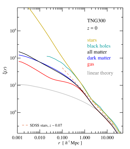
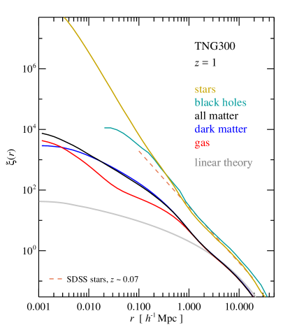
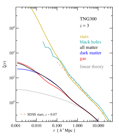
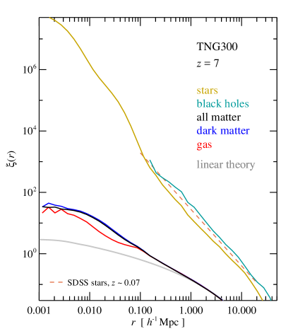
In Figure 1, we show the two-point correlation function of different matter components in the TNG300 simulation at redshifts , , and . We include results for the dark matter, the gas distribution, the star particles (i.e. the stellar mass), the black hole mass, and the total matter distribution. For comparison, the linear theory two-point correlation function is given at the corresponding redshifts as well.
Clear effects of non-linear evolution of the matter correlation function are visible for at , and they propagate with time to ever larger scales as the matter correlation function develops a characteristic ‘shoulder’ on small scales. As far as the dark matter goes, this can be explained in terms of the halo model (see Cooray & Sheth, 2002, for a review) where the clustering signal on small scales, below , is dominated by particle pairs in the same halo (‘one-halo term’), and the larger scale correlations come from pairs in different haloes (‘two-halo term’). Note that at the non-linear of the total matter distribution falls slightly below the linear theory at quasi-linear scales around . This happens despite the fact that the non-linear power spectrum is always larger than or equal to the linear power spectrum, and can occur for a limited range of due to the oscillatory factor in equation (11). This effect of non-linear evolution has already been seen in early N-body simulations (e.g. Ma, 1999) and can be interpreted in physical terms as a reflection of the depletion of matter on quasi-linear scales due to gravitational infall onto halos.
It is interesting that the baryonic gas starts to differ from the dark matter in the one-halo regime already early on. At redshift , the gas is actually more clustered than the dark matter on the smallest scales, while its clustering signal is slightly suppressed on intermediate scales. This changes qualitatively at low redshift, where the gas becomes less clustered than the dark matter also on small scales, and the overall suppression relative to dark matter becomes substantially larger. The strong small-scale clustering of the gas at , which dominates the matter power spectrum in this regime, reflects the intense cooling and star formation rates at this epoch, while the clustering deficit at late times is caused by the growing population of quenched, gas-poor galaxies that have depleted their gas reservoirs through star formation and expelled some of the baryons from their host haloes by feedback effects. Interestingly, this is at least qualitatively consistent with observational evidence for galaxies being baryon-dominated in their inner regions at the peak of galaxy formation activity (Genzel et al., 2017).
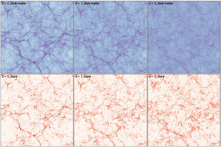
Another striking result is the very strong clustering of the stellar mass, which at low redshift is quite close to a power-law correlation function over a very large dynamic range. This clustering is nearly invariant in time, and for scales agrees very well with the power-law auto-correlation function of the stellar mass inferred by Li & White (2009) for the data release 7 of the Sloan Digital Sky Survey (SDSS) at a redshift of , which is reproduced as a dashed line in all the panels of Fig. 1. Although we find a clear steepening of the stellar mass auto-correlation towards smaller scales, this can be viewed as a first indication that the clustering of our simulated galaxies is in reasonably good agreement with observations. Also, it readily indicates that the bias of the stellar mass relative to the dark matter is large at high redshift, and then declines with time. This is also illustrated by the projected dark matter and stellar density fields shown in Figure 2 for the TNG300 simulation. The time evolution from to shows the gradual emergence of an ever more prominent cosmic web out of an initially nearly uniform dark matter distribution. In stark contrast, the stellar mass density field is highly structured already early on and evolves comparatively little with time.
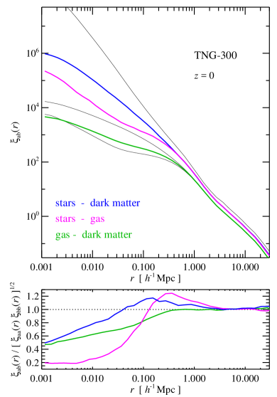
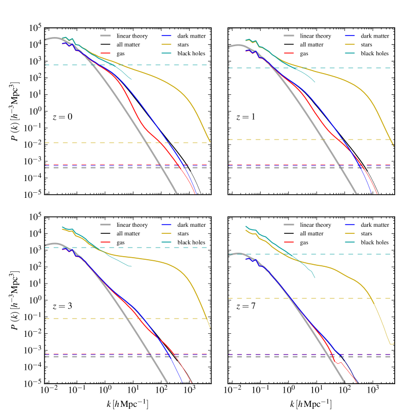
Figure 1 further shows that the clustering of the black hole mass in the simulations follows that of the stellar mass closely at , except on small scales, where the black hole two-point correlation function starts to fall short at and then suddenly drops to extremely low values for scales below about . This can be understood from the rapid merging of black hole pairs in our simulation model once they occupy the same halo. At the resolution of our simulations, the sinking of black holes to the potential minima of haloes due to dynamical friction cannot be followed accurately, hence we reposition black holes to the potential minimum of their host halo once they are close to the halo centre. This effectively assumes that dynamical friction is very efficient in bringing the black holes together, and that black hole binaries are formed quickly and then merge on a short time-scale. Towards higher redshifts, the corresponding influence on the clustering of black holes is expected to occur on slightly smaller scales due to the smaller sizes of haloes there, consistent with our results. We note that we use the ‘internal’ black hole mass (Springel et al., 2005a) associated with the sink particles for computing the clustering signal, not the sink’s inertial masses. These two can differ at high-redshift, where the seed black hole masses are smaller than our nominal baryonic resolution.
The clustering signal of the black holes is dominated by the most massive black holes, which have already grown significantly by gas accretion, greatly helping to limit the dependence of our black hole clustering results on the seeding prescription. Interestingly, the black hole mass exhibits a mild positive bias with respect to the stellar mass towards high redshift. This can be interpreted as a signature of top-down growth of black holes, where they first grow preferentially in more massive haloes than the stars, and hence end up being more strongly biased with respect to the matter. This difference tends to vanish towards the present epoch, at which point a largely universal ratio between stellar mass and black hole mass in galaxies is established.
In Figure 3, we consider the cross correlation functions between dark matter, gas and stars/black-holes333In this plot, we add the black hole mass to the stellar mass, for simplicity. at . The measured correlation functions fulfil the relationship
| (15) | |||||
by construction. The measurements demonstrate that all three mass components generally trace each other well, particularly on large scales. This can also be explicitly verified by considering a generalised correlation coefficient, such as the ratio
| (16) |
for dark matter and gas, and similarly for other pairs of matter components, as shown in the lower panel of Figure 3. For a simple linear bias, we expect , which is indeed achieved for all pairs of matter components on large scales. On smaller scales, the degree of correlation between the different fields becomes however weaker. Interestingly, at , the stars correlate better with dark matter than gas on halo scales and below, probably a reflection of the stronger alignment of the centrally concentrated distributions of stars with the dark matter cusps.
In Figure 4, we consider the power spectrum results for the same set of redshifts as shown in In Fig. 1. The qualitative behaviour of the different mass components is consistent with the real-space clustering discussed earlier. While the power spectra of the stars, black holes and the dark matter show comparatively little evolution between and , the gas actually shows a decrease in power at small and intermediate scales. This implies a non-monotonic evolution of the gas clustering with time, which can be interpreted as a signature of strong late-time feedback effects in the gas distribution. These results should be very informative for attempts to model the non-linear matter power spectra of stars and the gas phase analytically through extensions of the halo model (Fedeli, 2014; Fedeli et al., 2014).
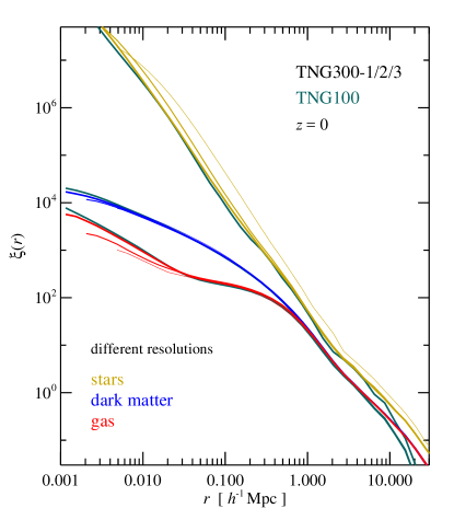
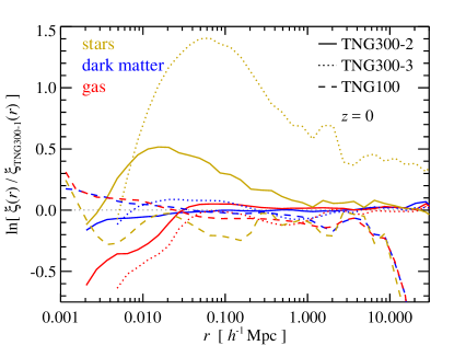
We examine the resolution dependence of our two-point correlation function estimates for the full physics simulation in Figure 5, separately for the stellar, dark matter and gaseous mass components. The clustering signal of the gas, dark matter, and stars is robustly reproduced even when varying the mass resolution by a factor of more than between TNG100-1 and TNG300-3, except for an excess of the clustering of the stars in the lowest resolution TNG300-3 simulation. In this calculation, star formation in low mass haloes is poorly resolved and anaemic, so that stars occupy preferentially more massive and rarer haloes that are more strongly biased. There are also some small differences between the runs close to the spatial resolution limits, which are of the expected magnitude. More importantly, the TNG100 model shows a significant deficit of clustering at very large scales, already setting in for . This is due to the limited box size of this simulation, which clearly affects the clustering on scales typically probed in galaxy surveys. The impact of the limited box size can be estimated by computing through equation (11), but restricting the integration to , i.e. modes represented in the box. This shows that the linear theory two-point correlation function of the TNG100 box size is expected to turn negative by , whereas the TNG300 simulation is affected only by 10% on this scale, and by much less on smaller scales. The correlation function of TNG300 turns negative at a scale of .
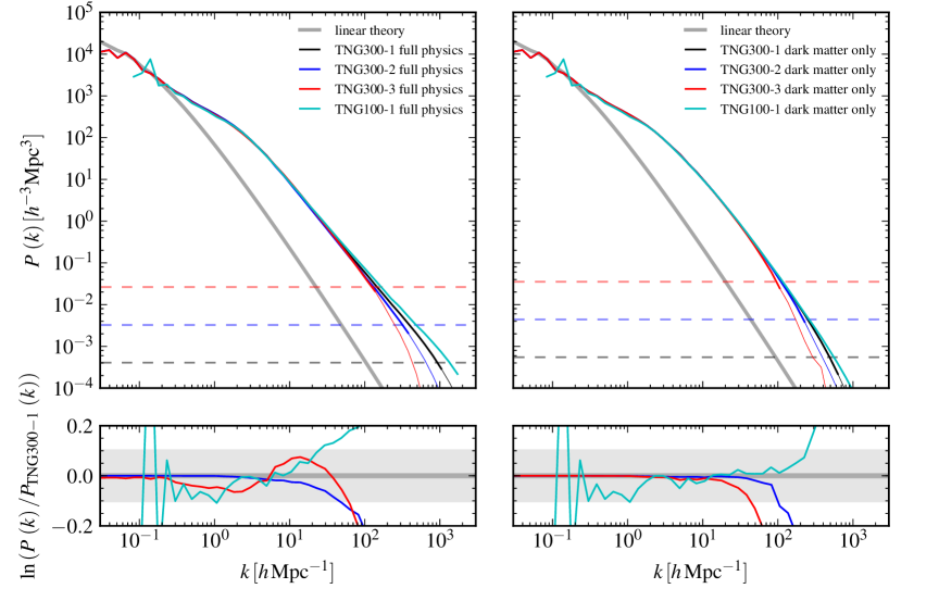
A corresponding analysis of the resolution dependence of the total matter power spectrum is given in Figure 6, with the left panel focusing on our full physics simulations while the right panel considers the corresponding dark matter only simulations. On large scales the power spectra agree very well, to better than 1% for scales down to a few times for the full physics simulations, and down to for the dark matter only runs.
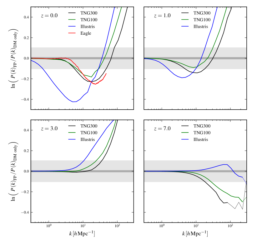
Given the numerical robustness of the large-scale clustering results, it is interesting to examine the overall impact of baryonic physics on the clustering of matter, which is arguably one of the most interesting effects that can be studied with hydrodynamic simulations, as highlighted first by van Daalen et al. (2011) and Semboloni et al. (2011). In Figure 7 we show the matter power spectrum of TNG300 relative to the corresponding one of the DM-only simulation, at redshifts , , , and . For comparison, we also include results for TNG100 and Illustris, as well as for the EAGLE simulation at (Hellwing et al., 2016). At the present epoch, the total change of the matter power spectrum is described by a characteristic suppression of power by at scales of , and a strong and rapidly rising enhancement of power setting in at scales around . The effect we see in IllustrisTNG is noticeably weaker than in Illustris, where the suppression extends to considerably larger scales (the scale for which the power is suppressed by more than 10% is almost an order of magnitude larger), and is stronger in amplitude, too. Interestingly, however, the effect in TNG is qualitatively similar to the EAGLE simulation (Hellwing et al., 2016), although it still is a bit stronger and extends to slightly larger scales. This is despite the fact that we use fundamentally different feedback prescriptions and numerical techniques, suggesting that the size of the expected AGN feedback impact is surprisingly robust to details of the modelling.
At higher redshifts, there are also some striking differences between Illustris and IllustrisTNG. Apparently, the modified AGN model and different wind parameterisation in these two simulations also affects the timing when the suppression of power on intermediate scales develops. In Illustris this emerges later than in the IllustrisTNG model.
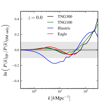
The modification of the total matter power spectrum in the full physics simulation is in part due to a redistribution of baryons by non-gravitational physics, and in part due to a change of the dark matter distribution as a result of the gravitational coupling to the baryons. In Figure 8, we look at the latter effect in isolation, at . The modification of the dark matter distribution alone is sizeable but overall weaker than that of the total matter, showing that the drastic change in the baryon distribution relative to the dark matter brought about by galaxy formation physics is a primary factor in determining the change of the total matter power spectrum. Interestingly, the dark matter clustering not only shows a damping on intermediate scales of , but also an enhancement of a few percent on times larger scales, around , where Illustris is still damped. The latter effect is nearly twice as large in EAGLE than in IllustrisTNG, but qualitatively the two simulations are relatively similar, and exhibit a significant difference to the much stronger effects in Illustris.
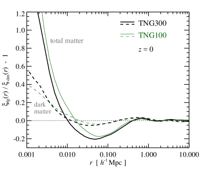
We can also consider the impact of baryonic effects on the two-point correlation function (see also van Daalen et al., 2014), which is shown in Figure 9 for TNG300 and TNG100 at . The predictions of both simulations agree very well given their substantial resolution and box size size differences. The solid lines report the relative change of the total matter clustering with respect to the clustering of the corresponding dark matter only simulation. The full physics simulations show a suppression of the clustering signal by about 20% on scales of , and a mild increase by about 5% at around . Part of these changes are due to a modification of the dark matter clustering itself, as shown by the dashed lines, but the relative clustering difference of the baryons is responsible for the bulk of the effect on small scales. At a distance scale of , the clustering of dark matter is increased by approximately 40% in the full physics calculations, while the total clustering strength is already more than twice as strong than in the corresponding dark matter only simulations.
4 The clustering of galaxies
IllustrisTNG predicts galaxies directly, in terms of gravitationally bound groups of stars that are identified by the SUBFIND algorithm (Springel et al., 2001). For each of these galaxies, we have obtained measurements of basic properties such as stellar mass, luminosity in different filter bands, morphology, size, or chemical abundances. Studying these properties of the predicted galaxy population lies traditionally at the heart of analysing hydrodynamical simulations of galaxy formation. Much less attention has thus far been given to analysing galaxy clustering in such simulations, in part due to the box size limitations discussed above.
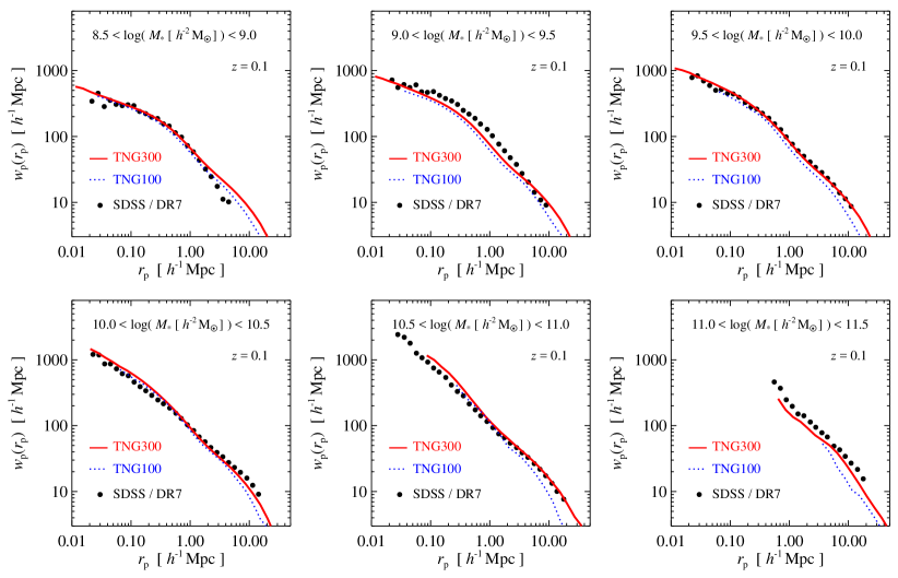
This makes it all the more interesting to consider the clustering of galaxies selected according to different criteria in our large volume TNG300 simulation, and to compare it to observational constraints from galaxy surveys. In Figure 10 we compare the galaxies at redshift to data from the Sloan Digital Sky Survey (SDSS), as compiled by Guo et al. (2010, 2011). The SDSS provides by far the most accurate characterisation of the low redshift galaxy distribution (Zehavi et al., 2011), and thus imposes stringent constraints on any galaxy formation model. We compare 6 bins of stellar mass to SDSS, finding in general rather reassuring agreement for the projected correlation functions, with a match of comparable quality to that of current physically based semi-analytic models of galaxy formation (Henriques et al., 2017; Kang, 2014) or stochastic HOD models (Zu & Mandelbaum, 2017). Also note that TNG300 and TNG100 agree rather well, except for large scales, , where TNG100 lies noticeably lower (an effect that is however expected due to the box size limitation of this simulation), and for the largest stellar mass sample, where we have too few galaxies in TNG100 to measure the correlation function for small separations. We are not aware that a similar degree of agreement in the clustering data over a comparably large dynamic range has ever been found for another hydrodynamic simulation of galaxy formation (see Artale et al., 2017, for one of the most succcessful other models).
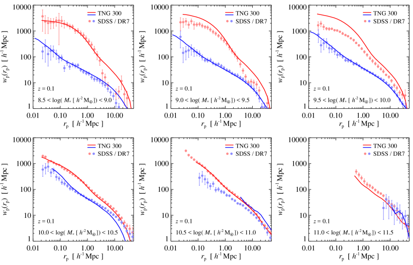
We extend this comparison by splitting up the samples in terms of galaxy colour in Figure 11, using the cut
| (17) |
to distinguish between red and blue galaxies. Colors are assigned using Bruzual & Charlot (2003) stellar populations synthesis models assuming a Charbrier IMF. This lies at the bottom of the valley separating the two populations and is similar to Henriques et al. (2017), but does not make any attempt to include dust corrections. The match to the blue galaxies is excellent, essentially for all stellar masses. The clustering of red galaxies appears slightly overestimated for intermediate stellar masses. We note however that the detailed size of this discrepancy depends on where the colour split is taken (see also the companion paper by Nelson et al., 2017), so we think this difference needs to be taken with a grain of salt. In general, however, we consider the level of agreement reassuring. It suggests that the quenching physics that operates in our hydrodynamical simulations in a self-consistent manner can broadly account for the observed clustering levels of red and blue galaxies, and their detailed variations with stellar mass, which is a non-trivial success. At the same time, the small residual differences can be used in the future to test extensions or modifications of the physics model implemented in the simulations.

In Figure 12, we consider clustering at much higher redshift of around , comparing different stellar mass samples of TNG300 to results published for the VIMOS VLT Deep Survey (VVDS, Meneux et al., 2008) and the DEEP2 galaxy redshift survey (Mostek et al., 2013). The clustering signal of the simulated galaxies agrees very well with DEEP2. However, while it appears close in shape to VVDS, it is clearly somewhat stronger than this survey, a finding similar to that reported by Meneux et al. (2008) for the Millennium simulation (Springel et al., 2005b), which shows a comparable excess. We note however that VVDS may be affected by cosmic variance due to the limited survey volume, and that the clustering lengths reported by the survey lie low compared to other surveys at similar redshift.
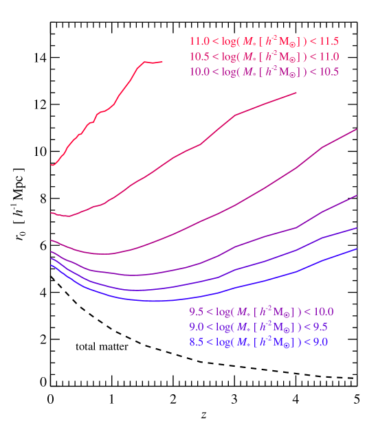
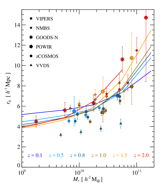
We make this more explicit in Figure 13, where we show the correlation length (defined as ) for different stellar mass samples from TNG300 as a function of redshift (left panel), or for samples at different redshift as a function of stellar mass (right panel). The latter is also compared to results reported for various galaxy surveys. Clearly, the clustering strength of the simulated galaxies is a strong function of stellar mass at any redshift. We note that the analysis of small-scale clustering of Artale et al. (2017) in EAGLE did not find any clear evidence for an increase of clustering strength with stellar mass or -band luminosity, in contrast to what we obtain here.
We also find that for a given stellar mass, the clustering length is a function of redshift, but depending on stellar mass, the evolution with redshift is not necessarily monotonic. For intermediate stellar masses, the clustering length first declines towards high redshift and then increases again, whereas for samples of very massive galaxies, it only increases towards higher redshift. The correlation length of the total matter, also included in Fig. 13 (left panel), behaves very differently and monotonically declines towards high redshift. Evidently, the bias between galaxies and matter is thus a strong function of redshift; it is generally high at early times, and then comes down and approaches values of order unity towards the present epoch.
It is interesting to compare various observational results for the clustering length to these simulation predictions, as we do in the right panel of Fig. 13. We consider data from VVDS (Meneux et al., 2008), the Palomar Observatory Wide-field Infrared Survey (POWIR Foucaud et al., 2010), VIPERS (Marulli et al., 2013), the NEWFIRM Medium Band Survey (NMBS Wake et al., 2011), GOODS-N (Lin et al., 2012), and zCOSMOS (Meneux et al., 2009). At a given stellar mass, our simulations predict only weak variations of clustering strength with redshift. For luminous galaxies with stellar mass above , the clustering strength increases towards higher redshift, a trend that is reversed for lower mass galaxies at low redshift. We find that our simulation predictions are broadly consistent with the data, which itself shows relatively large scatter, precluding any strong conclusions at this point about whether these subtle trends are also seen in the data. The theoretical results obtained here certainly provide strong motivation to start using the evolution of clustering length for specific galaxy samples as an important test of galaxy formation models.
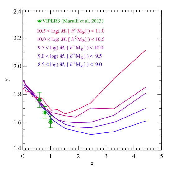
Many observational studies fit power-laws to the projected or real-space correlation functions in order to infer the correlation lengths and to represent the results in compact form. This is motivated by the close to power-law shape of the galaxy auto-correlation function at low redshift. In Figure 14, we show the power-law slope as a function of redshift obtained by fitting each of our measured galaxy correlation functions for different stellar mass samples, and at different redshifts, over the range . Strikingly, there is rather little dependence of the slope on stellar mass, at least at low redshift. The slope is at redshift , and then steepens to at . At intermediate redshifts, the low-mass stellar mass samples show somewhat shallower slopes than the galaxy samples with higher stellar mass, a difference that progressively becomes larger as they steepen again towards high redshift. When compared to observations, such as the VIPERS survey analysed in Marulli et al. (2013), we see that they show a very similar dependence of clustering slope on redshift. Interestingly this survey also failed to detect a significant stellar mass dependence of the slope for fixed redshift, which is quite consistent with our results.
5 Large-Scale Halo clustering
We now turn to an analysis of halo clustering, which is a central concept in empirical models for galaxy large-scale structure, such as HOD models, or more recently in SHAM models. It is generally believed that galaxies inherit the large-scale bias of their host halo, hence understanding halo bias is often used as a way to sidestep the issue of addressing galaxy bias directly. Recently, Jose et al. (2016) formulated a model for the scale-dependence of halo bias which offers the prospect to also extend this to quasi-linear scales.
It has long been realised that dark matter haloes more massive than the characteristic halo mass are positively biased with respect to the matter, and less massive haloes exhibit a negative bias. This can be understood based on the clustering of peaks in Gaussian random fields. Similar to derivations of the halo mass function, this gives rise to analytic models for halo bias. This is concisely expressed in the model of Mo & White (1996), which determines the halo bias in terms of peak height, making the theoretical prediction in principle universal and independent of redshift. Many N-body simulations have been used to test this prediction, generally finding that it works quite well, but with some residual discrepancies that motivate the development of improved models (e.g. Sheth & Tormen, 1999; Pillepich et al., 2010; Tinker et al., 2010).
The situation is reminiscent of the halo mass function, where the basic spherically symmetric formulation by Press & Schechter (1974) provides a decent first order approximation that can be substantially improved by models of ellipsoidal collapse (Sheth et al., 2001). However, the latter still shows some discrepancies compared to N-body simulations, which can be addressed through empirical fitting functions to the numerical results (e.g. Jenkins et al., 2001).
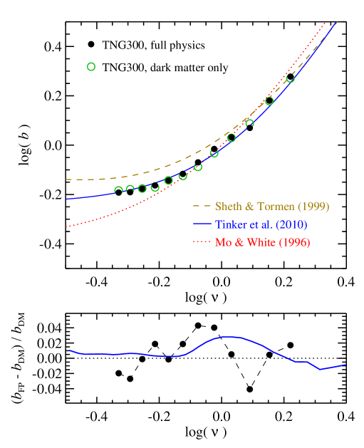
In Figure 15, we show the linear halo bias on the largest scales, as a function of peak height, in the form it has been analysed in a large number of cold dark matter simulation studies. We include results for the full physics run of TNG300 (filled circles), and for the dark matter only version of the same model (open circles). For comparison, we also show the predictions of Mo & White (1996), Sheth & Tormen (1999), and Tinker et al. (2010). The latter provides clearly a very good fit to our results. The differences between the full physics simulation and the dark matter only results are displayed in the lower panel of Fig. 15, and are quite small. There are some systematic distortions in the halo bias of up to 3% induced by baryonic physics. We argue that these changes can be largely explained by a modification of the halo masses themselves. For example, when feedback effects expel gas from a halo, its mass is lowered and its subsequent non-linear growth can be slowed as well. The associated initial density fluctuation peak is not changed by this, however. Knowing this halo mass change quantitatively (which we determine below), we can predict the expected change of halo bias as a function of peak height, based on the model of Tinker et al. (2010). The result of this is shown as a solid line in the lower panel of Figure 15. While this does not reproduce the (somewhat noisy) measurements in detail, the predicted effect is of very similar magnitude to the one measured, suggesting that this is indeed the dominating effect.
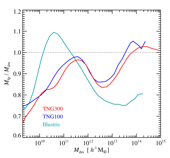
This estimate has made use of the results of Figure 16, where we show the mass change of haloes due to the inclusion of baryonic physics. To this end we compare the masses of haloes at equal comoving abundance in corresponding pairs of full physics and dark matter only simulations. This is simply achieved by sorting the haloes by mass in descending order, and then comparing them at equal rank, a procedure that yields very similar (albeit not identical) outcomes to cross-matching haloes by the particle-IDs of their dark matter content. We include results for TNG300, TNG100 and the Illustris simulation. In TNG, a particularly strong impact of baryonic physics occurs for halo masses around , which is due to the comparatively sudden onset of strong kinetic-mode AGN feedback, as can be verified through the increase of the associated energy input in galaxies of the associated stellar mass (Weinberger et al., 2017a). However, consistent with the reduced impact of baryonic physics on the power spectra, we find that the TNG model shows overall a much weaker impact on halo masses than the Illustris feedback model (see also Vogelsberger et al., 2014b). In particular, the suppression of halo masses due to AGN feedback sets in at higher masses, and is restricted to a narrower mass range, with poor clusters of galaxies already being largely unaffected. On the other hand, in the halo mass range , the TNG model shows a stronger effect on its halo masses than Illustris, reflecting its modified wind model. Looking also at the results for other feedback implementations (Velliscig et al., 2014), is therefore clear that the variation of halos masses depends quite sensitively on the employed feedback model.
6 Scale-dependent Bias
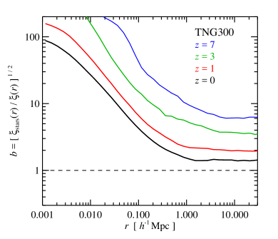
In Figure 17, we consider the bias of all the stellar mass in our TNG300 simulation relative to the total matter, here in terms of the real-space clustering. This corresponds to for the results in Fig. 1. We clearly see the very large positive bias of about at the highest examined redshift, which then progressively comes down towards the present epoch. At , the bias of the stellar mass is still positive with a value of about . Interestingly, the scale-dependence of this bias sets in earlier (i.e. on larger scales) at high redshift than at low redshift.
A scale-dependent bias can be a great challenge for the interpretation of galaxy redshift surveys. Such a scale-dependence will naturally arise from mild quasi-linear and fully non-linear evolution, but even when the bias is considered relative to the non-linearly evolved density field, it is not clear a priori up to which scales galaxies can be used as faithful tracers for the mass distribution by simply invoking the value of the linear bias on the largest scales. Another complication is that the bias is expected to strongly depend on the sample selection procedure. Tracers with the same number density but of different type can exhibit substantially different biases, and can also be affected to different degrees by scale-dependence.
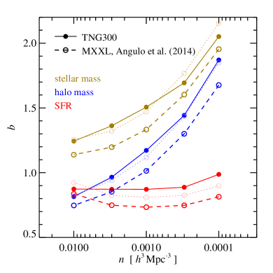
In Figure 18, we demonstrate the dependence on tracer type explicitly by showing the linear bias on large scales as a function of tracer number density, for three different selection criteria. In particular, we consider haloes according to their virial mass (), galaxies selected by their stellar mass (), and galaxies selected by their instantaneous star formation rate (). In each case, the objects are sorted in descending order and included top down until the corresponding space density is reached. Remarkably, the galaxies selected according to their star formation rates show only a very weak variation of their bias (which is in fact an anti-bias) with tracer density. This shows that these galaxies do not tend to populate the most massive haloes – which makes sense because these haloes are often quenched and hence are not natural hosts of star-forming galaxies. In contrast, galaxies selected by stellar mass show a large positive bias that increases strongly towards more luminous systems. This reflects the trend of higher bias values for rarer and hence more massive haloes.
We have compared our results in Fig. 18 to a similar analysis carried out by Angulo et al. (2014) for the Millennium-XXL simulation (Angulo et al., 2012) on the basis of a semi-analytic galaxy formation model. There is good qualitative agreement, but our bias values are systematically higher. Most of the difference can simply be explained by the higher value of adopted in Angulo et al. (2014). As the clustering pattern of a given tracer evolves comparatively little in time, whereas the dark matter auto-correlation on large scales grows according to linear theory, we can to first order correct for this by comparing to an earlier output of Millennium-XXL when its normalization corresponds to our value of . Or simpler still, we can adjust their bias results by a factor of , thus effectively bringing the MXXL’s dark matter correlation function to the less evolved state corresponding to our simulation. This yields the dotted results in Fig. 18, which are in good agreement with TNG300.
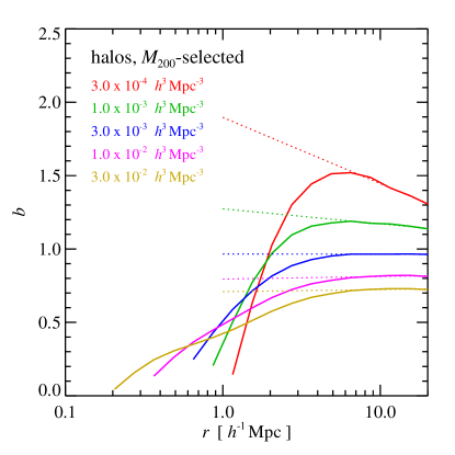
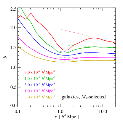
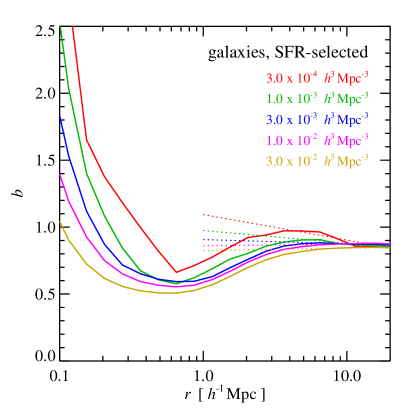
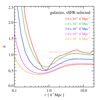
Instead of just looking at the linear bias on the largest scales, it is much more interesting to consider the bias of different tracers also as a function of scale. We do this in Figure 19 for the real-space two-point correlation function. Again, we consider tracers with different space densities, with five values ranging from to , using a selection by halo mass, galaxy stellar mass, instantaneous star formation rate, and current specific star formation rate (). For our TNG300 volume, the samples then contain 2585 objects at a space density of , and 258454 at the highest considered density of . We note that these space densities cover the range considered in a number of ongoing or planned large galaxy surveys that target cosmology, hence we expect effects of similar magnitude in real galaxy surveys. For definiteness, for the halo samples the limiting values of the five considered space densities are , , , , and , respectively. For the stellar mass samples, the limiting values are , , , , and . The selection according to star formation rate corresponds to limiting values of , , , and . Finally, the specific star formation rate selection is based on cut-off values of , , , and .
For the halo samples in Fig. 19, the bias of the two-point correlation functions shows a clear short-range exclusion effect, with the bias function suddenly dropping precipitously and rapidly towards short distances. Halo samples dominated by relatively low mass haloes show no significant scale dependence for , but more massive haloes do. A similar behaviour is found for the stellar mass samples, except that on scales of a mild decrease of the bias is seen, followed by a strong rise towards small scales. The bias at a given space density for samples selected by stellar mass is always much higher than for haloes, and also when galaxies are selected by star formation rate or specific star formation rate. For the latter two samples, the dip in bias at intermediate scales and the small-scale rise are much more pronounced than for halo or stellar mass samples.
We now turn to the question of whether such scale dependent biases also affect the baryonic acoustic oscillations (BAOs). These are an important cosmological resource, and in particular a primary observational handle to constrain the cosmic expansion history and thus models of dark energy. Detecting the BAOs not just in the cosmic microwave background but also in galaxy surveys or quasar absorption line studies at intervening redshifts is therefore a major goal in observational cosmology (e.g. Eisenstein et al., 2005; Cole et al., 2005; Wang et al., 2017).
Our TNG300 simulation box is just large enough to see the baryonic acoustic oscillations (BAO) in the total matter power spectrum, but the number of available large-scale modes over the relevant range is too small to directly measure the oscillations with the required accuracy for cosmological inferences. However, we can still measure the power spectra of different tracers and determine their bias relative to the non-linear matter power spectrum. Taking the ratio of the two power spectra eliminates much of the cosmic variance fluctuations due to the specific realisation of our large-scale modes. The result is seen in Figure 20, where we show our bias measurements for two different space densities, and , and for tracers selected by halo virial mass, galaxy stellar mass, and galaxy star formation rate. We include results for redshifts , , and .
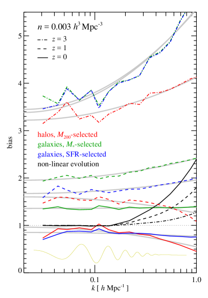
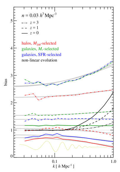
Again, it is evident from the results that the bias depends strongly on tracer type, redshift, and space density. Interestingly, over the -range of the baryonic acoustic oscillations (indicated as thin yellow lines in Fig. 20), clear variations of the measured bias values are detected. To quantify this scale dependence over the range , we fit our measurements with a very simple scale-dependent bias model of the form
| (18) |
Here represents the large-scale linear bias, while measures the strength of the scale dependence. We set in our fits so that at . The resulting smooth bias laws are shown with thick grey lines in the figure, and the corresponding fit parameters are given in Table 2. The very good statistics we have for the full matter distribution also allows us to reliably measure the ratio of the full matter power spectrum relative to the linear theory power spectrum. This is shown as black lines in Fig. 20 for redshifts , , and , and can be interpreted as an effective bias that encodes the non-linear clustering evolution. The bias of a tracer sample relative to the linear theory power spectrum is then the product of this effective bias with the intrinsic bias of the tracers.
We can use these results to obtain an estimate of the distortion of the BAO features in the matter power spectrum due to non-linear evolution and scale-dependent biases. This is shown in Figure 21, where we modify the linear theory power spectrum by the effective bias encoding non-linear evolution, and the scale-dependent bias for three example tracers from Fig. 20. We show in each case the estimated evolved power spectrum divided by a smoothed, wiggle-free linear theory power spectrum, in order to bring out the BAOs more clearly. We stress that this estimate only accounts for effects of non-linear evolution at the level of the mean power per mode. In reality, mode-coupling effects will tend to wash out and broaden the BAO features, and can even give rise to additional small shifts in the peak positions. This is not accounted for in our simple illustrative analysis shown in Fig. 21, but this effect can be relatively well understood for the dark matter density field based on renormalised perturbation theory (Crocce & Scoccimarro, 2008).
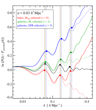
Even though we have refrained from including in Fig. 21 the tracer samples with the strongest scale-dependent biases (which occur for massive or star-forming galaxies at ) and neglected mode-mode coupling, the distorting effect on the BAO features is substantial. In particular, the -positions of the local maxima of the peaks are shifted by several percent, and depending on the precise tracer or redshift considered, the shift can be both positive or negative. Superficially, this may sound like very bad news for the cosmological use of the BAO features. However, these shifts can be corrected for by fitting the observed BAO features with the expected signal template (e.g. Seo et al., 2008; Angulo et al., 2014; Prada et al., 2016). For example, one could use a simple model of the form
| (19) |
where , , and are fit parameters. The describe a polynomial fit to the scale-dependent bias that is empirically determined from the data, while is a stretch factor that is supposed to pick up a real shift of the acoustic scale, if it exits.
Fitting such a model to the distorted BAOs of Figure 21 indeed recovers values that are very close to unity: in the case of the halo sample we obtain , for the stellar mass selected galaxies , and for the SFR-selected sample . The reason why this works so well is that the scale-dependent bias we detect and the effects of non-linear evolution vary smoothly with scale. When one knows what to look for, then they can be taken out very well. And in our case, we have prescribed the expected linear theory template precisely, without any measurement errors and without a damping of the higher order wiggles by non-linear evolution.
For real data, the conditions are not nearly as favourable, making the possible systematic impact of scale-dependent bias on BAO studies still an interesting research question. At the very least, it is to be expected that there will be a small impact on the constraining power of observational surveys (e.g. Amendola et al., 2017). The ability of our simulation models to make accurate predictions for galaxy bias should help precise characterisations of such effects. This however requires a proper modelling of effects such as mode-mode coupling, redshift space distortions, and observational errors and selection effects, which is beyond the scope of this paper.
7 Discussion and Conclusions
In this study, we have analysed the matter and galaxy clustering in a new suite of high-resolution hydrodynamical calculations of galaxy formation, the IllustrisTNG simulations. Besides numerous improvements in the treatment of feedback effects and in the numerical accuracy of the simulations, an important advance of IllustrisTNG lies in its push to higher volume, allowing a more faithful sampling of the halo and galaxy distribution including rarer objects, and in particular, a much better representation of cosmic large-scale structure. The latter is probed in powerful ways by current and upcoming galaxy redshift surveys (such as EUCLID, DES, or eBOSS). The precision with which theoretical galaxy formation models can explain the clustering of galaxies as a function of stellar mass, colour, star formation, redshift, etc., offers the prospect to constrain and test such models in interesting ways, as well as lifting possible modeling degeneracies. At the same time, clustering data is a critical component of modern cosmological constraints, including those that seek to tie down the cosmic expansion history and inform about the nature of dark energy. Here simulation predictions can inform about possible observational biases and help to eliminate them.
| sample | |||||||
|---|---|---|---|---|---|---|---|
| 0.003 | |||||||
| SFR | |||||||
| 0.03 | |||||||
| SFR | |||||||
Thus far, hydrodynamical simulations of galaxy formation have been severely challenged even by the basic task to reliably predict the clustering length, simply due to the missing large-scale power as a result of small simulated volumes. TNG300 is advancing the state of the art in this regard. At its mass resolution, no other hydrodynamical simulation of comparable volume and with a similar coverage of the physics exists, opening up the possibility for quantitative studies of large-scale structure, a regime that was thus far almost exclusively in the domain of semi-analytic models of galaxy formation, or empirical approaches such as HOD or SHAM. This also means that the approximate nature of these treatments can finally be tested with full hydrodynamical simulations.
We note that the IllustrisTNG simulations not only make extant predictions for the clustering of point objects such as galaxies and haloes, but also for the distribution of gas and the stellar mass, as well as, of course, for the total matter. This includes the impact of baryonic effects on the dark matter distribution, something that is difficult if not impossible to forecast with any degree of reliability by (semi-)analytic models. Predicting these effects reliably is of significant importance for the analysis of gravitational lensing, for studying the circumgalactic medium around galaxies, and for interpreting the population of intrahalo stars.
With TNG300, we have been able to provide accurate measurements of the non-linear matter power spectra and correlation functions of different mass components over a large dynamic range. We have highlighted the strong bias of the stellar light relative to the total matter, and the fact that its two-point correlation function is nearly invariant in time and close to a power-law. This prediction appears to be fairly robust to resolution and likely represents a generic feature of CDM cosmologies.
We have also shown that the galaxy distribution predicted by IllustrisTNG clusters very similarly to observations by the Sloan Digital Sky Survey at low redshift, both as a function of stellar mass and galaxy colour. This is an important confirmation of the basic validity of our hydrodynamical simulation models, and together with the findings of our companion papers, underlines that IllustrisTNG provides a powerful, self-consistent model for how galaxies have emerged in the CDM cosmology.
With this basic confirmation in hand, we have explored other clustering predictions from our simulations. The observational picture of how galaxy clustering measured in terms of clustering length and slope of the two-point functions depends on redshift and stellar mass has been somewhat muddled. TNG300 makes clear statements in this regard, showing that clustering length is a strong function of stellar mass at all redshifts, whereas the clustering slope is not. The latter tends to get a bit shallower towards and hardly depends on stellar mass over this range at all, just to become steeper again towards high redshift and also showing again a stellar mass dependence there.
Our analysis of galaxy and halo bias has shown that our results on the largest scales are consistent with those obtained from simpler dark matter only simulations. This is reassuring and largely to be expected, given that effects of baryonic physics are restricted to show up on intermediate and small scales. However, many observational data sets lose significant power if their analysis is restricted to scales that are safely unaffected by scale-dependent effects. Such scale-dependent biases are clearly detected in our simulations, extending out to the scales of the baryonic acoustic oscillations. These scale-dependent biases strongly depend on the type of tracer that is used, the sample selection criterion, the space-density that is used, and the redshift. They originate from a complex coupling of weakly non-linear evolution and galaxy formation physics, something that is accounted for naturally in our simulations. It has yet to be seen how sensitively some of these bias predictions depend on details of the galaxy formation physics, but if there is a chance at all to calculate them reliably, it is through hydrodynamical simulations such as the ones discussed here.
One of the most interesting possible effects of a scale-dependent bias is that it may impact measurements of the baryonic acoustic oscillations based on the low-redshift galaxy distribution. When done in real space, the baryonic acoustic peak has been shown to be remarkably resilient to galaxy formation physics effects (e.g. Angulo et al., 2014), but the BAO features in Fourier-space are more drawn out in scale and thus potentially more sensitive to distortions from a scale-dependent bias.
While our TNG300 simulation box is just large enough to cover the scales of the baryonic acoustic oscillations in the total matter power spectrum, the number of available large-scale modes is unfortunately too small to measure these weak power fluctuations directly. However, measurements of the scale-dependent bias of different tracers on these scales are much less affected by cosmic variance, as this involves dividing out the specific realisation of the total matter power spectrum. In this way, we could demonstrate a significant scale-dependence of the bias of different tracers over the range of the BAOs, and also quantify the size of non-linear evolution effects over this region. Combining both allows an estimate of the BAO distortions in the evolved power spectrum as seen through the tracers. We have found in this way significant shifts of the BAO peak positions of up to 6% in , but template fitting of the expected wiggle signal appears capable of eliminating such apparent shifts of the acoustic scale, thereby preventing being misled in the cosmological interpretation.
Hydrodynamical simulations of still larger volumes will be able in the near future to substantially improve the statistics of our results on large scales, circumventing the significant approximations involved in other approaches to study cosmic large-scale structure and BAO distortions from biased tracers. This offers the exciting prospect that detailed hydrodynamical simulations of galaxy formation become an integral and powerful part of forthcoming cosmological precision studies.
Acknowledgements
We thank the anonymous referee for an insightful report. We thank Hellwing Wojciech for making the EAGLE power spectrum ratio available in electronic form. VS, RP, and RW acknowledge support through the European Research Council under ERCStG grant EXAGAL-308037, and would like to thank the Klaus Tschira Foundation. The IllustrisTNG flagship simulations were run on the HazelHen Cray XC40 supercomputer at the High-Performance Computing Center Stuttgart (HLRS) as part of project GCS-ILLU of the Gauss Centre for Supercomputing (GCS). VS also acknowledges support through subproject EXAMAG of the Priority Programme 1648 ‘Software for Exascale Computing’ of the German Science Foundation. MV acknowledges support through an MIT RSC award, the support of the Alfred P. Sloan Foundation, and support by NASA ATP grant NNX17AG29G. JPN acknowledges support of NSF AARF award AST-1402480. SG and PT acknowledge support from NASA through Hubble Fellowship grants HST-HF2-51341.001-A and HST-HF2-51384.001-A, respectively, awarded by the STScI, which is operated by the Association of Universities for Research in Astronomy, Inc., for NASA, under contract NAS5-26555. The Flatiron Institute is supported by the Simons Foundation. Ancillary and test runs of the project were also run on the compute cluster operated by HITS, on the Stampede supercomputer at TACC/XSEDE (allocation AST140063), at the Hydra and Draco supercomputers at the Max Planck Computing and Data Facility, and on the Harvard computing facilities supported by FAS.
References
- Amendola et al. (2017) Amendola L., Menegoni E., Di Porto C., Corsi M., Branchini E., 2017, Phys. Rev. D, 95, 023505
- Angulo et al. (2012) Angulo R. E., Springel V., White S. D. M., Jenkins A., Baugh C. M., Frenk C. S., 2012, MNRAS, 426, 2046
- Angulo et al. (2014) Angulo R. E., White S. D. M., Springel V., Henriques B., 2014, MNRAS, 442, 2131
- Artale et al. (2017) Artale M. C., et al., 2017, MNRAS, 470, 1771
- Bardeen et al. (1986) Bardeen J. M., Bond J. R., Kaiser N., Szalay A. S., 1986, ApJ, 304, 15
- Behroozi et al. (2010) Behroozi P. S., Conroy C., Wechsler R. H., 2010, ApJ, 717, 379
- Benson (2012) Benson A. J., 2012, New Astron., 17, 175
- Berlind & Weinberg (2002) Berlind A. A., Weinberg D. H., 2002, ApJ, 575, 587
- Bond et al. (1996) Bond J. R., Kofman L., Pogosyan D., 1996, Nature, 380, 603
- Bray et al. (2016) Bray A. D., et al., 2016, MNRAS, 455, 185
- Bruzual & Charlot (2003) Bruzual G., Charlot S., 2003, MNRAS, 344, 1000
- Campbell et al. (2017) Campbell D., van den Bosch F. C., Padmanabhan N., Mao Y.-Y., Zentner A. R., Lange J. U., Jiang F., Villarreal A., 2017, preprint, (arXiv:1705.06347)
- Cattaneo et al. (2017) Cattaneo A., et al., 2017, MNRAS, 471, 1401
- Chaves-Montero et al. (2016) Chaves-Montero J., Angulo R. E., Schaye J., Schaller M., Crain R. A., Furlong M., Theuns T., 2016, MNRAS, 460, 3100
- Clay et al. (2015) Clay S. J., Thomas P. A., Wilkins S. M., Henriques B. M. B., 2015, MNRAS, 451, 2692
- Cole et al. (2005) Cole S., et al., 2005, MNRAS, 362, 505
- Colombi et al. (2009) Colombi S., Jaffe A., Novikov D., Pichon C., 2009, MNRAS, 393, 511
- Cooray & Sheth (2002) Cooray A., Sheth R., 2002, Phys. Rep., 372, 1
- Crain et al. (2017) Crain R. A., et al., 2017, MNRAS, 464, 4204
- Crocce & Scoccimarro (2008) Crocce M., Scoccimarro R., 2008, Phys. Rev. D, 77, 023533
- Croton et al. (2016) Croton D. J., et al., 2016, ApJS, 222, 22
- Davis & Peebles (1983) Davis M., Peebles P. J. E., 1983, ApJ, 267, 465
- Davis et al. (1985) Davis M., Efstathiou G., Frenk C. S., White S. D. M., 1985, ApJ, 292, 371
- De Lucia et al. (2006) De Lucia G., Springel V., White S. D. M., Croton D., Kauffmann G., 2006, MNRAS, 366, 499
- DeGraf & Sijacki (2017) DeGraf C., Sijacki D., 2017, MNRAS, 466, 3331
- Desjacques et al. (2016) Desjacques V., Jeong D., Schmidt F., 2016, preprint, (arXiv:1611.09787)
- Dolag et al. (2016) Dolag K., Komatsu E., Sunyaev R., 2016, MNRAS, 463, 1797
- Dubois et al. (2016) Dubois Y., Peirani S., Pichon C., Devriendt J., Gavazzi R., Welker C., Volonteri M., 2016, MNRAS, 463, 3948
- Eisenstein et al. (2005) Eisenstein D. J., et al., 2005, ApJ, 633, 560
- Fedeli (2014) Fedeli C., 2014, J. Cosmology Astropart. Phys., 4, 028
- Fedeli et al. (2014) Fedeli C., Semboloni E., Velliscig M., Van Daalen M., Schaye J., Hoekstra H., 2014, J. Cosmology Astropart. Phys., 8, 028
- Fisher et al. (1994) Fisher K. B., Davis M., Strauss M. A., Yahil A., Huchra J. P., 1994, MNRAS, 267, 927
- Foucaud et al. (2010) Foucaud S., Conselice C. J., Hartley W. G., Lane K. P., Bamford S. P., Almaini O., Bundy K., 2010, MNRAS, 406, 147
- Gao et al. (2005) Gao L., Springel V., White S. D. M., 2005, MNRAS, 363, L66
- Geller & Huchra (1989) Geller M. J., Huchra J. P., 1989, Science, 246, 897
- Genel et al. (2014) Genel S., et al., 2014, MNRAS, 445, 175
- Genzel et al. (2017) Genzel R., et al., 2017, Nature, 543, 397
- Guo et al. (2010) Guo Q., White S., Li C., Boylan-Kolchin M., 2010, MNRAS, 404, 1111
- Guo et al. (2011) Guo Q., et al., 2011, MNRAS, 413, 101
- Guo et al. (2016) Guo Q., et al., 2016, MNRAS, 461, 3457
- Hearin et al. (2016) Hearin A. P., Zentner A. R., van den Bosch F. C., Campbell D., Tollerud E., 2016, MNRAS, 460, 2552
- Hellwing et al. (2016) Hellwing W. A., Schaller M., Frenk C. S., Theuns T., Schaye J., Bower R. G., Crain R. A., 2016, MNRAS, 461, L11
- Henriques et al. (2015) Henriques B. M. B., White S. D. M., Thomas P. A., Angulo R., Guo Q., Lemson G., Springel V., Overzier R., 2015, MNRAS, 451, 2663
- Henriques et al. (2017) Henriques B. M. B., White S. D. M., Thomas P. A., Angulo R. E., Guo Q., Lemson G., Wang W., 2017, MNRAS, 469, 2626
- Jenkins et al. (1998) Jenkins A., et al., 1998, ApJ, 499, 20
- Jenkins et al. (2001) Jenkins A., Frenk C. S., White S. D. M., Colberg J. M., Cole S., Evrard A. E., Couchman H. M. P., Yoshida N., 2001, MNRAS, 321, 372
- Jose et al. (2016) Jose C., Lacey C. G., Baugh C. M., 2016, MNRAS, 463, 270
- Kaiser (1984) Kaiser N., 1984, ApJ, 284, L9
- Kang (2014) Kang X., 2014, MNRAS, 437, 3385
- Katz et al. (1999) Katz N., Hernquist L., Weinberg D. H., 1999, ApJ, 523, 463
- Kauffmann (2015) Kauffmann G., 2015, MNRAS, 454, 1840
- Kauffmann et al. (1993) Kauffmann G., White S. D. M., Guiderdoni B., 1993, MNRAS, 264, 201
- Kauffmann et al. (1999) Kauffmann G., Colberg J. M., Diaferio A., White S. D. M., 1999, MNRAS, 303, 188
- Khandai et al. (2015) Khandai N., Di Matteo T., Croft R., Wilkins S., Feng Y., Tucker E., DeGraf C., Liu M.-S., 2015, MNRAS, 450, 1349
- Lacey et al. (2016) Lacey C. G., et al., 2016, MNRAS, 462, 3854
- Li & White (2009) Li C., White S. D. M., 2009, MNRAS, 398, 2177
- Lin et al. (2012) Lin L., et al., 2012, ApJ, 756, 71
- Ma (1999) Ma C.-P., 1999, ApJ, 510, 32
- Marinacci et al. (2017) Marinacci F., et al., 2017, preprint, (arXiv:1707.03396)
- Marulli et al. (2013) Marulli F., et al., 2013, A&A, 557, A17
- Masaki et al. (2013) Masaki S., Lin Y.-T., Yoshida N., 2013, MNRAS, 436, 2286
- Meneux et al. (2008) Meneux B., et al., 2008, A&A, 478, 299
- Meneux et al. (2009) Meneux B., et al., 2009, A&A, 505, 463
- Mo & White (1996) Mo H. J., White S. D. M., 1996, MNRAS, 282, 347
- Mostek et al. (2013) Mostek N., Coil A. L., Cooper M., Davis M., Newman J. A., Weiner B. J., 2013, ApJ, 767, 89
- Moster et al. (2010) Moster B. P., Somerville R. S., Maulbetsch C., van den Bosch F. C., Macciò A. V., Naab T., Oser L., 2010, ApJ, 710, 903
- Moster et al. (2017) Moster B. P., Naab T., White S. D. M., 2017, preprint, (arXiv:1705.05373)
- Naiman et al. (2017) Naiman J. P., et al., 2017, preprint, (arXiv:1707.03401)
- Nelson et al. (2015) Nelson D., et al., 2015, Astronomy and Computing, 13, 12
- Nelson et al. (2017) Nelson D., et al., 2017, preprint, (arXiv:1707.03395)
- Nuza et al. (2010) Nuza S. E., Dolag K., Saro A., 2010, MNRAS, 407, 1376
- Pakmor & Springel (2013) Pakmor R., Springel V., 2013, MNRAS, 432, 176
- Pakmor et al. (2011) Pakmor R., Bauer A., Springel V., 2011, MNRAS, 418, 1392
- Pakmor et al. (2014) Pakmor R., Marinacci F., Springel V., 2014, ApJ, 783, L20
- Pakmor et al. (2016) Pakmor R., Springel V., Bauer A., Mocz P., Munoz D. J., Ohlmann S. T., Schaal K., Zhu C., 2016, MNRAS, 455, 1134
- Peacock & Smith (2000) Peacock J. A., Smith R. E., 2000, MNRAS, 318, 1144
- Peebles (1980) Peebles P. J. E., 1980, The large-scale structure of the universe. Princeton University Press
- Pillepich et al. (2010) Pillepich A., Porciani C., Hahn O., 2010, MNRAS, 402, 191
- Pillepich et al. (2017) Pillepich A., et al., 2017, preprint, (arXiv:1707.03406)
- Pillepich et al. (2018) Pillepich A., et al., 2018, MNRAS, 473, 4077
- Planck Collaboration et al. (2016) Planck Collaboration et al., 2016, A&A, 594, A13
- Prada et al. (2016) Prada F., Scóccola C. G., Chuang C.-H., Yepes G., Klypin A. A., Kitaura F.-S., Gottlöber S., Zhao C., 2016, MNRAS, 458, 613
- Press & Schechter (1974) Press W. H., Schechter P., 1974, ApJ, 187, 425
- Pujol et al. (2017) Pujol A., et al., 2017, MNRAS, 469, 749
- Sánchez et al. (2006) Sánchez A. G., Baugh C. M., Percival W. J., Peacock J. A., Padilla N. D., Cole S., Frenk C. S., Norberg P., 2006, MNRAS, 366, 189
- Schaye et al. (2015) Schaye J., et al., 2015, MNRAS, 446, 521
- Semboloni et al. (2011) Semboloni E., Hoekstra H., Schaye J., van Daalen M. P., McCarthy I. G., 2011, MNRAS, 417, 2020
- Seo et al. (2008) Seo H.-J., Siegel E. R., Eisenstein D. J., White M., 2008, ApJ, 686, 13
- Sheth & Tormen (1999) Sheth R. K., Tormen G., 1999, MNRAS, 308, 119
- Sheth et al. (2001) Sheth R. K., Mo H. J., Tormen G., 2001, MNRAS, 323, 1
- Smith et al. (2007) Smith R. E., Scoccimarro R., Sheth R. K., 2007, Phys. Rev. D, 75, 063512
- Somerville et al. (2008) Somerville R. S., Hopkins P. F., Cox T. J., Robertson B. E., Hernquist L., 2008, MNRAS, 391, 481
- Springel (2010) Springel V., 2010, MNRAS, 401, 791
- Springel et al. (2001) Springel V., White S. D. M., Tormen G., Kauffmann G., 2001, MNRAS, 328, 726
- Springel et al. (2005a) Springel V., Di Matteo T., Hernquist L., 2005a, MNRAS, 361, 776
- Springel et al. (2005b) Springel V., et al., 2005b, Nature, 435, 629
- Springel et al. (2006) Springel V., Frenk C. S., White S. D. M., 2006, Nature, 440, 1137
- Tegmark et al. (2004) Tegmark M., et al., 2004, ApJ, 606, 702
- Tinker et al. (2010) Tinker J. L., Robertson B. E., Kravtsov A. V., Klypin A., Warren M. S., Yepes G., Gottlöber S., 2010, ApJ, 724, 878
- Velliscig et al. (2014) Velliscig M., van Daalen M. P., Schaye J., McCarthy I. G., Cacciato M., Le Brun A. M. C., Dalla Vecchia C., 2014, MNRAS, 442, 2641
- Vogelsberger et al. (2013) Vogelsberger M., Genel S., Sijacki D., Torrey P., Springel V., Hernquist L., 2013, MNRAS, 436, 3031
- Vogelsberger et al. (2014a) Vogelsberger M., et al., 2014a, MNRAS, 444, 1518
- Vogelsberger et al. (2014b) Vogelsberger M., et al., 2014b, Nature, 509, 177
- Wake et al. (2011) Wake D. A., et al., 2011, ApJ, 728, 46
- Wang et al. (2013) Wang L., Weinmann S. M., De Lucia G., Yang X., 2013, MNRAS, 433, 515
- Wang et al. (2017) Wang Y., et al., 2017, MNRAS, 469, 3762
- Wechsler et al. (2006) Wechsler R. H., Zentner A. R., Bullock J. S., Kravtsov A. V., Allgood B., 2006, ApJ, 652, 71
- Weinberg et al. (2004) Weinberg D. H., Davé R., Katz N., Hernquist L., 2004, ApJ, 601, 1
- Weinberger et al. (2017a) Weinberger R., et al., 2017a, preprint, (arXiv:1710.04659)
- Weinberger et al. (2017b) Weinberger R., et al., 2017b, MNRAS, 465, 3291
- White et al. (1987) White S. D. M., Frenk C. S., Davis M., Efstathiou G., 1987, ApJ, 313, 505
- Yang et al. (2006) Yang X., Mo H. J., van den Bosch F. C., 2006, ApJ, 638, L55
- Zehavi et al. (2011) Zehavi I., et al., 2011, ApJ, 736, 59
- Zentner et al. (2014) Zentner A. R., Hearin A. P., van den Bosch F. C., 2014, MNRAS, 443, 3044
- Zu & Mandelbaum (2015) Zu Y., Mandelbaum R., 2015, MNRAS, 454, 1161
- Zu & Mandelbaum (2017) Zu Y., Mandelbaum R., 2017, preprint, (arXiv:1703.09219)
- de la Torre et al. (2011) de la Torre S., et al., 2011, MNRAS, 412, 825
- van Daalen et al. (2011) van Daalen M. P., Schaye J., Booth C. M., Dalla Vecchia C., 2011, MNRAS, 415, 3649
- van Daalen et al. (2014) van Daalen M. P., Schaye J., McCarthy I. G., Booth C. M., Dalla Vecchia C., 2014, MNRAS, 440, 2997
- van Daalen et al. (2016) van Daalen M. P., Henriques B. M. B., Angulo R. E., White S. D. M., 2016, MNRAS, 458, 934