Solving PDE problems with uncertainty using neural-networks

Abstract

The curse of dimensionality is commonly encountered in numerical partial differential equations (PDE), especially when uncertainties have to be modeled into the equations as random coefficients. However, very often the variability of physical quantities derived from a PDE can be captured by a few features on the space of the coefficient fields. Based on such an observation, we propose using a neural-network (NN) based method to parameterize the physical quantity of interest as a function of input coefficients. The representability of such quantity using a neural-network can be justified by viewing the neural-network as performing time evolution to find the solutions to the PDE. We further demonstrate the simplicity and accuracy of the approach through notable examples of PDEs in engineering and physics.

1 Introduction

Uncertainty quantifications in physical and engineering applications often involve the study of partial differential equations (PDE) with random coefficient field. To understand the behavior of a system in the presence of uncertainties, one can extract PDE-derived physical quantities as functionals of the coefficient fields. This can potentially require solving the PDE an exponential number of times numerically even with a suitable discretization of the PDE domain, and of the range of random variables. Fortunately in most PDE applications, often these functionals depend only on a few characteristic “features” of the coefficient fields, allowing them to be determined from solving the PDE a limited number of times.

A commonly used approach for uncertainty quantifications is Monte-Carlo sampling. An ensemble of solutions is built by repeatedly solving the PDE with different realizations of the coefficient field. Then physical quantities of interest, for example, the mean of the solution at a given location, can be computed from the ensemble of solutions. Although being applicable in many situations, the computed quantity is inherently noisy. Moreover, this method lacks the ability to obtain new solutions if they are not sampled previously. Other approaches exploit the low underlying dimensionality assumption in a more direct manner. For example the stochastic Galerkin method [17, 20] expands the random solution using certain prefixed basis functions (i.e. polynomial chaos [22, 23]) on the space of random variables, thereby reducing the high dimensional problem to a few deterministic PDEs. Such type of methods requires careful treatment of the uncertainty distributions, and since the basis used is problem independent, the method could be expensive when the dimensionality of the random variables is high. There are data-driven approaches for basis learning such as applying Karhunen-Loève expansion to PDE solutions from different realizations of the PDE [4]. Similarly to the related principal component analysis, such linear dimension-reduction techniques may not fully exploit the nonlinear interplay between the random variables. At the end of day, the problem of uncertainty quantification is one of characterizing the low-dimensional structure of the coefficient field that gives the observed quantities.

On the other hand, the problem of dimensionality reduction has been central to the fields of statistics and machine learning. The fundamental task of regression seeks to find a function $h_{\theta}$ parameterized by a parameter vector $\theta\in\mathbb{R}^{p}$ such that

$$f(a)\approx h_{\theta}(a),\ a\in\mathbb{R}^{q}.$$ (1)

However, choosing a sufficiently large class of approximation functions without the issue of over-fitting remains a delicate business, for example when choosing the set of basis $\{\phi_{k}(a)\}$ such that $f(a)=\sum_{k}\beta_{k}\phi_{k}(a)$ in linear regression. In the last decade, deep neural-networks have demonstrated immense success in solving a variety of difficult regression problems related to pattern recognitions [10, 15, 19]. A key advantage of using neural-network is that it bypasses the traditional need to handcraft basis for spanning $f(a)$ as in linear regression but instead, directly learns an approximation that satisfies (1) in a data-driven way. The performance of neural-network in machine learning applications, and more recently in physical applications such as representing quantum many-body states (e.g. [3, 21]), encourages us to study its use in the context of solving PDE with random coefficients. More precisely, we want to learn $f(a)$ that maps the random coefficient vector $a$ in a PDE to some physical quantities described by the PDE.

Our approach to solving quantities arise from PDE with randomness is conceptually simple, consisting of the following steps:

• Sample the random coefficients ($a$ in (1)) of the PDE from a user-specified distribution. For each set of coefficients, solve the deterministic PDE to obtain the physical quantity of interest ($f(a)$ in (1)).

• Use a neural-network as the surrogate model $h_{\theta}(a)$ in (1) and train it using the previously obtained samples.

• Validate the surrogate forward model with more samples. The neural network is now ready for applications.

Though being a simple method, to the best of our knowledge, dimension reduction based on neural-network representation has not been adapted to solving PDE with uncertainties. We demonstrate the success of neural-network in two important PDEs that have wide applications in physics and engineering. In particular, we consider solving for the effective conductance in inhomogeneous media and the ground state energy of a nonlinear Schrödinger equation (NLSE) having inhomogeneous potential. These quantities are $f$ in (1) that we want to learn as a function of $a$, where $a$ is the random conductivity coefficient or the random potential. The main contributions of our work are

• We provide theoretical guarantees on neural-network representation of $f(a)$ through explicit construction for the parametric PDE problems under study;

• We show that even a rather simple neural-network architecture can learn a good representation of $f(a)$ through training.

We note that our work is different from [7, 12, 13, 16, 18], which solve deterministic PDE numerically using a neural-network. The goal of these works is to parameterize the solution of a deterministic PDE using neural-network and use optimization methods to solve for the PDE solution. It is also different from [8] where a deterministic PDE is solved as a stochastic control problem using neural-network. In this paper, the function that we want to parameterize is over the coefficient field of the PDE.

The advantages of having an explicitly parameterized approximation to $f(\cdot)$ are numerous, which we will only list a couple here. First, the neural-network parameterized function can serve as a surrogate forward model for generating samples cheaply for statistical analysis. Second, the task of optimizing some function of the physical quantity with respect to the PDE coefficients in engineering design problems can be done with the help of a gradient calculated from the neural-network. To summarize, obtaining a neural-network parametrization could limit the use of expensive PDE solvers in applications.

The paper is organized as followed. In Section 2, we provide background on the two PDEs of interest. In Section 3, the theoretical justification of using NN to represent the physical quantities derived from the PDEs introduced in Section 2, is provided. In Section 4, we describe the neural-network architecture for handling these PDE problems and report the numerical results. We finally conclude in Section 5.

2 Two examples of parametric PDE problems

This section introduces the two PDE models – the linear elliptic equation [14] and the nonlinear Schrödinger equation [11] – we want to solve for. Elliptic equations are commonly used to study steady heat conduction in a given material. When the material has inhomogeneities (modeled as random conductivity coefficients in the elliptic equation), one typically wants to understand the effective conductivity of the material. NLSE is used to understand light propagation in waveguide and also the quantum mechanical phenomena where bosonic particles highly concentrate in the lowest-energy state (Bose-Einstein condensation). We want to study how the energy of such ground state behaves when the NLSE is subjected to random potential field. Therefore, we focus on the map from the coefficient field of these PDEs to their relevant physical quantities. In both of the PDEs, the boundary condition is taken to be periodic for simplicity.

2.1 Effective coefficients for inhomogeneous elliptic equation

Our first example will be finding the effective conductance/coefficient in a non-homogeneous media. For this, we consider a class of coefficient functions

$$\mathcal{A}=\{a\in L^{\infty}([0,1]^{d})\mid\lambda_{1}\geq a(x)\geq\lambda_{0}>0\},$$ (2)

for some fixed constants $\lambda_{0}$ and $\lambda_{1}$. Fix a direction $\xi\in\mathbb{R}^{d}$ with $\|\xi\|_{2}=1$ ($\|\cdot\|_{2}$ is the Euclidean norm). We want to obtain the effective conductance functional $A_{\mathrm{eff}}:\mathcal{A}\rightarrow\mathbb{R}$ defined by

$$A_{\mathrm{eff}}(a)=\min_{u(x)}\int_{[0,1]^{d}}a(x)\|\nabla u(x)+\xi\|_{2}^{2}\,\mathrm{d}x.$$ (3)

The minimizer $u_{a}(x)$ of this variational problem (here the subscript “$a$” in $u_{a}$ is used to denote its dependence on the coefficient field $a$) satisfies the following elliptic partial different equation

$$-\nabla\cdot\left(a(x)(\nabla u(x)+\xi)\right)=0,\quad x\in[0,1]^{d}$$ (4)

with periodic boundary condition. With $u_{a}$ available, one obtains

$$A_{\mathrm{eff}}(a)=\int_{[0,1]^{d}}a(x)\|\nabla u_{a}(x)+\xi\|_{2}^{2}\,\mathrm{d}x.$$

In practice, to parameterize ${A}_{\mathrm{eff}}$ as a functional of the coefficient field $a(\cdot)$, we discretize the domain using a uniform grid with step size $h=1/n$ and grid points denoted by $x_{i}=ih$, where the multi-index $i\in\{(i_{1},\ldots,i_{d})\},1\leq i_{1},\ldots,i_{d}\leq n$. In this way, we can think about the coefficient field $a(x)$ and the solution $u(x)$ represented on the grid points both as vectors with length $n^{d}$. More precisely, we redefine

$$\mathcal{A}=\{a\in\mathbb{R}^{n^{d}}\mid a_{i}\in[\lambda_{0},\lambda_{1}],\,\forall i\}$$

and discretize the term $-\nabla\cdot\left(a(x)\nabla u(x)\right)$ using central difference

$$-\sum_{k=1}^{d}\frac{a_{i+e_{k}/2}(u_{i+e_{k}}-u_{i})-a_{i-e_{k}/2}(u_{i}-u_{i-e_{k}})}{h^{2}},$$ (5)

for each $i$, where $\{e_{k}\}_{k=1}^{d}$ denotes the canonical basis in $\mathbb{R}^{d}$ and each value of $a$ at a half grid point is obtained by averaging the values at its two nearest grid points. Then the discrete version of (4) is the linear system $L_{a}u=b_{a}$ with

$$(L_{a}u)_{i}:=\sum_{k=1}^{d}\frac{-a_{i+e_{k}/2}u_{i+e_{k}}+(a_{i-e_{k}/2}+a_{i+e_{k}/2})u_{i}-a_{i-e_{k}/2}u_{i-e_{k}}}{h^{2}}$$ (6)

$$(b_{a})_{i}:=\sum_{k=1}^{d}\frac{\xi_{k}(a_{i+e_{k}/2}-a_{i-e_{k}/2})}{h}.$$ (7)

From (3), one can see that the discrete version of the effective conductivity, also denoted by $A_{\mathrm{eff}}(a)$ for $a\in\mathbb{R}^{n^{d}}$, can be obtained from solving the discrete variational problem

$$A_{\mathrm{eff}}(a)=2\min_{u\in\mathbb{R}^{n^{d}}}\mathcal{E}(u;a),\quad\mathcal{E}(u;a):=\frac{h^{d}}{2}(u^{\top}L_{a}u-2u^{\top}b_{a}+a^{\top}\mathbf{1}),$$ (8)

or equivalently, solving $u_{a}$ from $L_{a}u=b_{a}$ and setting

$$A_{\mathrm{eff}}(a)=h^{d}(u_{a}^{\top}L_{a}u_{a}-2u_{a}^{\top}b_{a}+a^{\top}\mathbf{1}).$$

We stress that in order to simplify the notations, we use $u$ and $a$ as vectors in $\mathbb{R}^{n^{d}}$, although they were previously used as functions in (3). The interpretation of $u$ and $a$ as functions or vectors should be clear from the context.

2.2 NLSE with inhomogeneous background potential

For the second PDE example, we want to find the ground state energy $E_{0}$ of a nonlinear Schrödinger equation with potential $a(x)$:

$$-\Delta u(x)+a(x)u(x)+\sigma u(x)^{3}=E_{0}u(x),\quad x\in[0,1]^{d},\\ \text{s.t.}\ \int_{[0,1]^{d}}u(x)^{2}\,\mathrm{d}x=1.$$ (9)

We take $\sigma=2$ in this work and thus consider a defocusing cubic Schrödinger equation, which can be understood as a model for soliton in nonlinear photonics or Bose-Einstein condensate with inhomogeneous media. Similar to (6), we solve the discretized version of the NLSE

$$(Lu)_{i}+a_{i}u_{i}+\sigma u_{i}^{3}=E_{0}u_{i},\quad\sum_{i=1}^{n^{d}}u_{i}^{2}h^{d}=1,\quad(Lu)_{i}:=\sum_{k=1}^{d}\frac{-u_{i+e_{k}}+2u_{i}-u_{i-e_{k}}}{h^{2}}.$$ (10)

Due to the nonlinear cubic term, it is more difficult to solve for the NLSE numerically compare to (4). Therefore in this case, the value of having a surrogate model of $E_{0}$ as a function of $a$ is more significant. We note that the solution $u$ to (10) (and thus $E_{0}$) can also be obtained from the following variational problem

$$\min_{u\in\mathbb{R}^{n^{d}}:\,\|u\|_{2}^{2}=n^{d}}u^{\top}Lu+u^{\top}\text{diag}(a)u+\frac{\sigma}{2}\sum_{i}u_{i}^{4},$$ (11)

where the $\text{diag}(\cdot)$ operator forms a diagonal matrix given a vector.

3 Theoretical justification of deep neural-network representation

The physical quantities introduced in Section 2 are determined through the solution of the PDEs given the coefficient field. Rather than solving the PDE, we will prove that the map from coefficient field to such quantities can be represented using convolutional NNs. The main idea is to view the solution $u$ of the PDE as being obtained via time evolution, where each layer of the NN corresponds to the solution at discrete time step. In other words, mapping the input $a$ from the first layer to last layer in the NN resembles the time-evolution of a PDE with discrete time-steps. We focus here on the case of solving elliptic equations with inhomogeneous coefficients. Similar line of reasoning can be used to demonstrate the representability of the ground state-energy $E_{0}$ as a function of $a$ using an NN.

Theorem 1.

Fix an error tolerance $\epsilon>0$, there exists a neural-network $h_{\theta}(\cdot)$ with $O(n^{d})$ hidden nodes per-layer and $O((\frac{\lambda_{1}}{\lambda_{0}}+1)\frac{n^{2}}{\epsilon})$ layers such that for any $a\in\mathcal{A}=\{a\in\mathbb{R}^{n^{d}}\mid a_{i}\in[\lambda_{0},\lambda_{1}],\,\forall i\}$, we have

$$\lvert h_{\theta}(a)-A_{\mathrm{eff}}(a)\rvert\leq\epsilon\lambda_{1}.$$ (12)

Note that due to the ellipticity assumption $a\in\mathcal{A}$, the effective conductivity is bounded from below by $A_{\mathrm{eff}}(a)\geq\lambda_{0}>0$. Therefore the theorem immediately implies a relative error bound

$$\frac{\lvert h_{\theta}(a)-A_{\mathrm{eff}}(a)\rvert}{A_{\mathrm{eff}}(a)}\leq\epsilon\frac{\lambda_{1}}{\lambda_{0}}.$$ (13)

We illustrate the main idea of the proof in the rest of the section, the technical details of the proof are deferred to the supplementary materials.

The first observation is that, due to the variational characterization (8), in order to get $A_{\mathrm{eff}}(a)$ we may minimize $\mathcal{E}(u;a)$ over the solution space $u$, using e.g., steepest descent:

$$u^{m+1} =u^{m}-\Delta t\frac{\partial\mathcal{E}(u^{m};a)}{\partial u}$$ (14)

$$=u^{m}-\Delta t\bigl{(}L_{a}u^{m}-b_{a}\bigr{)},$$

where $\Delta t$ is a step size chosen sufficiently small to ensure descent of the energy. Note that the optimization problem is convex due to the ellipticity assumption (2) of the coefficient field $a$ (which ensures $u^{\top}L_{a}u>0$ except for $u=\mathbf{1}$) with Lipshitz continuous gradient, therefore the iterative scheme converges to the minimizer with proper choice of step size for any initial condition. Thus we can choose $u^{0}=0$.

Now we identify the iteration scheme in (14) with a convolutional NN architecture (Fig. 1) by viewing $m$ as an index of the NN layers. The input of the NN is the vector $a\in\mathbb{R}^{n^{d}}$, and the hidden layers are used to map between the consecutive pairs of $(d+1)$-tensors $U^{m}_{i_{0}i_{1}\ldots i_{d}}$ and $U^{m+1}_{i_{0}i_{1}\ldots i_{d}}$. The zeroth dimension for each tensor $U^{m}$ is the channel dimension and the last $d$ dimensions are the spatial dimensions. If we let the channels in each $U^{m}$ be consisted of a copy of $a$ and a copy of $u^{m}$, e.g., let

$$U^{m}_{0i_{1}\ldots i_{d}}=a_{(i_{1},\ldots,i_{d})},\quad U^{m}_{1i_{1}\ldots i_{d}}=u^{m}_{(i_{1},\ldots,i_{d})},$$ (15)

in light of (14) and (6), one simply needs to perform local convolution (to aggregate $a$ locally) and nonlinearity (to approximate quadratic form of $a$ and $u^{m}$) to get from $U^{m}_{1i_{1}\ldots i_{d}}=u^{m}_{(i_{1},\ldots,i_{d})}$ to $U^{m+1}_{1i_{1}\ldots i_{d}}=u^{m+1}_{(i_{1},\ldots,i_{d})}$; while the $0$-channel is simply copied to carry along the information of $a$. Stopping at $m=M$ layer and letting $u^{M}$ be the approximate minimizer of $\mathcal{E}(u;a)$, based on (8), we let $\mathcal{E}(u^{M};a)$ be an approximation to $A_{\mathrm{eff}}(a)$. This architecture of NN to approximate the effective conductance is illustrated in Fig. 1. Note that the architecture of NN used in the proof resembles a deep ResNet [9], as the coefficient field $a$ is passed from the first to the last layer. The detailed estimates of the approximation error and the number of parameters will be deferred to the supplementary materials.

Let us point out that if we take the continuum time limit of the steepest descent dynamics, we obtain a system of ODE

$$\partial_{t}u=-(L_{a}u-b_{a}),$$ (16)

which can be viewed as a spatially discretized PDE. Thus our construction of the neural network in the proof is also related to the work [16] where multiple layers of convolutional NN is used to learn and solve evolutionary PDEs. However, the goal of the neural network here is to approximate the physical quantity of interest as a functional of the (high-dimensional) coefficient field, which is quite different from the view point of [16].

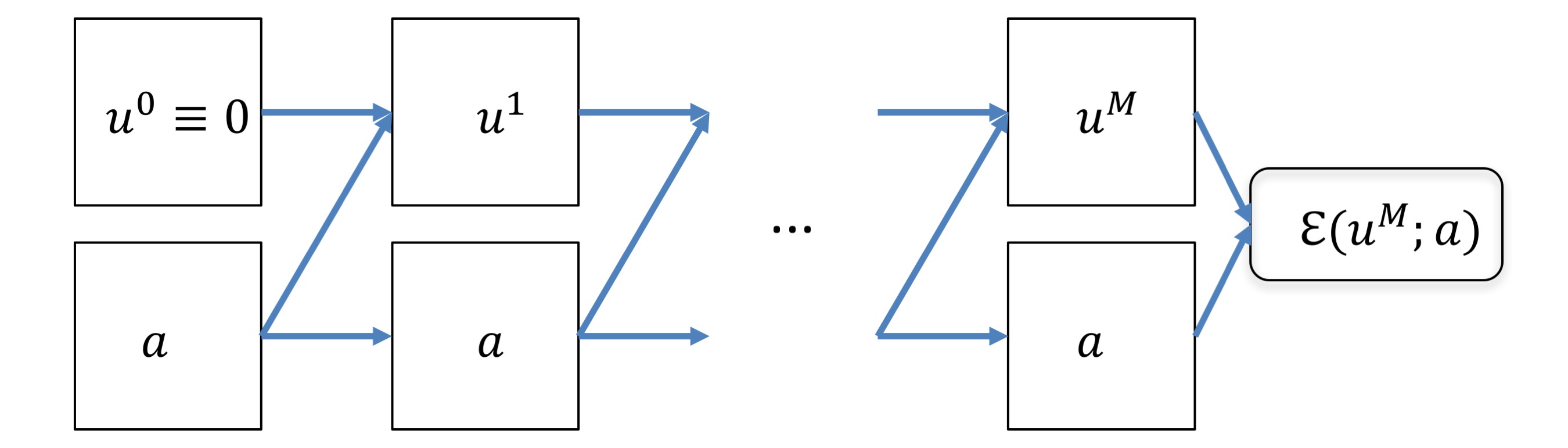
Figure 1: Construction of the NN in the proof of Theorem 1. The NN takes the coefficient field $a$ as an input and the convolutional and local nonlinearity layers are used to map from $u^{m},a$ to $u^{m+1},a$, $m=0,M-1$. At $u_{M}$, local convolutions and nonlinearity are used to obtained $\mathcal{E}(u^{M};a)$.

We also remark that the number of layers of the NN required by Theorem 1 is rather large. This is due to the choice of the (unconditioned) steepest descent algorithm as the engine of optimization to generate the neural network architecture used in the proof. Nevertheless, the number of parameters required in the NN representation is still much fewer than the exponential scaling in terms of the input dimension of a shallow network [2] from universal approximation theorem. Moreover, with a better preconditioner such as the algebraic multigrid [24] for the gradient, we can effectively reduce the number of layers to $O(1)$ and thus achieves an optimal count of parameters involved in the NN; the details will be left for future works. In practice, as shown in the next section by actual training of parametric PDEs, the neural network architecture can be much simplified while maintaining a good approximation to the quantity of interest.

4 Proposed network architecture and numerical results

In this section, based on the discussion in Section 3, we propose using convolutional NN to approximate the physical quantities given by the PDE with a periodic boundary condition. We first describe the architecture of the neural network in Section 4.1, then the implementation details and numerical results are provided in Section 4.2 and 4.3 respectively.

4.1 Architecture

In Fig. 2, we show the architecture for the 2D case with domain being a unit square, though it can be generalized to solving PDEs in any dimensions. The input to the NN is an $n\times n$ matrix representing the coefficient field $a\in\mathbb{R}^{n^{2}}$ on grid points, and the output of the network gives physical quantity of interest from the PDE. The main part of the network are convolutional layers with ReLU being the nonlinearity. This extracts the relevant features of the coefficient field around each grid point that contribute to the final output. The use of a sum-pooling followed by a linear map to obtain the final output is based on the translational symmetry of the function $f(\cdot)$ to be represented. More precisely, let $a^{\tau_{1}\tau_{2}}_{ij}:=a_{(i+\tau_{1})(j+\tau_{2})}$ where the additions are done on $\mathbb{Z}_{n}$. The output of the convolutional layer gives basis functions that satisfy

$$\tilde{\phi}_{kij}(a^{\tau_{1}\tau_{2}})=\tilde{\phi}_{k(i-\tau_{1})(j-\tau_{2})}(a),\quad k=1,\ldots,\alpha,\ i,j=1,\ldots,n,\ \forall\tau_{1},\tau_{2}=1,\ldots,n.$$ (17)

When using the architecture in Fig. 2, for any $\tau_{1},\tau_{2}$,

$$f(a^{\tau_{1}\tau_{2}}) = \sum_{k=1}^{\alpha}\beta_{k}\sum_{i=1}^{n}\sum_{j=1}^{n}\bigg{(}\tilde{\phi}_{kij}(a^{\tau_{1}\tau_{2}})\bigg{)}=\sum_{k=1}^{\alpha}\beta_{k}\sum_{i=1}^{n}\sum_{j=1}^{n}\bigg{(}\tilde{\phi}_{k(i-\tau_{1})(j-\tau_{2})}(a)\bigg{)}$$ (18)

$$= \sum_{k=1}^{\alpha}\beta_{k}\phi_{k}(a),\quad\phi_{k}:=\sum_{i=1}^{n}\sum_{j=1}^{n}\tilde{\phi}_{kij},$$ (19)

where $\beta_{k}$’s are the weights of the last densely connected layer. The summation over $i,j$ comes from the sum-pooling operation. Therefore, (18) shows that the translational symmetry of $f$ is preserved.

We note that all operations in Fig. 2 are standard except the padding operation. Typically, zero-padding is used to enlarge the size of the input in image classification task, whereas we extend the input periodically due to the assumed periodic boundary condition.

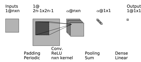
Figure 2: Single convolutional layer neural network for representing translational invariant function.

4.2 Implementation

The neural-network is implemented using Keras [5], an application programming interface running on top of TensorFlow [1] (a library of toolboxes for training neural-network). We use a mean-squared-error loss function. The optimization is done using the NAdam optimizer [6]. The hyper-parameter we tune is the learning rate, which we lower if the training error fluctuates too much. The weights are initialized randomly from the normal distribution. The input to the neural-network is whitened to have unit variance and zero-mean on each dimension. The mini-batch size is always set to between 50 and 200.

4.3 Numerical examples

4.3.1 Effective conductance

For the case of effective conductance, we assume the entries $a_{i}$’s of $a\in\mathbb{R}^{n^{d}}$ are independently and identically distributed according to $\mathcal{U}[0.3,3]$ where $\mathcal{U}[\lambda_{0},\lambda_{1}]$ denotes the uniform distribution on the interval $[\lambda_{0},\lambda_{1}]$. The results of learning the effective conductance function are presented in Table 1. To get the training samples, we solve the linear system in (6). We use the same number of samples for training and validation. Both the training and validation error are measured by

$$\sqrt{\frac{\sum_{k}(h_{\theta}(a^{k})-A_{\mathrm{eff}}(a^{k}))^{2}}{\sum_{k}A_{\mathrm{eff}}(a^{k})^{2}}},$$ (20)

where $a^{k}$’s can either be the training or validation samples sampled from the same distribution and $h_{\theta}$ is the neural-network-parameterized approximation function. We remark that although incorporating domain knowledge in PDE to build a sophisticated neural-network architecture would likely boost the approximation quality, such as what we do in the constructive proof for Theorem 1, our results in Table 1 show that even a simple network as in Fig. 2 can already give decent results with near $10^{-3}$ accuracy. The simplicity of the NN is particularly important when using it as a surrogate model of the PDE to generate samples cheaply.

Table 1: Error in approximating the effective conductance function $A_{\mathrm{eff}}(a)$ in 2D. The mean and standard deviation of the effective conductance are computed from the samples in order to show the variability. The sample sizes for training and validation are the same.

$n$	$\alpha$	Training error	Validation error	Average $A_{\mathrm{eff}}$	No. of samples	No. of parameters
8	16	$2.4\times 10^{-3}$	$3.0\times 10^{-3}$	$1.86\pm 0.10$	$1.2\times 10^{4}$	1057
16	16	$2.1\times 10^{-3}$	$2.2\times 10^{-3}$	$1.87\pm 0.052$	$2.4\times 10^{4}$	4129

Before concluding this subsection, we use the exercise of determining the effective conductance in 1D to provide another motivation for the usage of a neural-network. Unlike the 2D case, in 1D the effective conductance can be expressed analytically as the harmonic mean of $a_{i}$’s:

$$A_{\mathrm{eff}}(a)=\biggl{(}\frac{1}{n}\sum_{i=1}^{n}\frac{1}{a_{i}}\biggr{)}^{-1}.$$ (21)

This function indeed approximately corresponds to the deep neural-network shown in Fig. 3. The neural-network is separated into three stages. In the first stage, the approximation to function $1/a_{i}$ is constructed for each $a_{i}$ by applying a few convolution layers with size $1$ kernel window. In this stage, the channel size for these convolution layers is chosen to be 16 except the last layer since the output of the first stage should be a vector of size $n$. In the second stage, a layer of sum-pooling with size $n$ window is used to perform the summation in (21), giving a scalar output. The third and first stages have the exact same architecture except the input to the third stage is a scalar. $2560$ samples are used for training and another $2560$ samples are used for validation. We let $a_{i}\sim\mathcal{U}[0.3,1.5]$, giving an effective conductance of $0.77\pm 0.13$ for $n=8$. We obtain $4.9\times 10^{-4}$ validation error with the neural-network in Fig. 3 while with the network in Fig. 2, we get $5.5\times 10^{-3}$ accuracy with $\alpha=16$. As a check, in Fig. 4 we show that the output from the first stage is well-fitted by the reciprocal function.

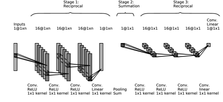
Figure 3: Neural-network architecture for approximating $A_{\mathrm{eff}}(a)$ in the 1D case. Although the layers in third stage are essentially densely-connected layers, we still identify them as convolution layers to reflect the symmetry between the first and third stages.

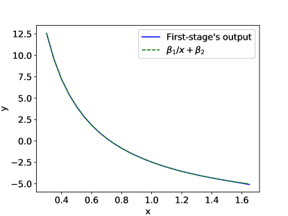
Figure 4: The first stage’s output of the neural-network in Fig. 3 fitted by $\beta_{1}/x+\beta_{2}$. The training result agrees well with the analytical structure of the solution to the 1D effective conductance.

4.3.2 Ground state energy of NLSE

We next focus on the 2D NLSE example (10) with $\sigma=2$. The goal here is to obtain a neural-network parametrization for $E_{0}(a)$, with input now being $a\in\mathbb{R}^{n^{2}}$ with i.i.d. entries distributed according to $\mathcal{U}[1,16]$. As mentioned before, solving for the ground state energy in NLSE is more expensive than solving for the effective conductance as in this case, we need to solve a system of nonlinear equations. In order to generate training samples, for each realization of $a$, the nonlinear eigenvalue problem (10) is solved via a homotopy method. In such method, a sequence of NLSE $Lu+a_{i}u_{i}+su_{i}^{3}=E_{0}u_{i}\ \forall i$ with the normalization constraint on $u$ is solved with $s=s_{1},\ldots,s_{K}$ where $0=s_{1}<s_{2}<\ldots<s_{K}=\sigma$. First, the case $s=0$ is solved as a standard eigenvalue problem. Then for each $s_{i}$ with $i>1$, Newton’s method is used to solved the NLSE and $u,E_{0}$ obtained with $s=s_{i}$ will be used to warm start the Newton’s iteration for $s_{i+1}$. In our example, we change $s$ from 0 to 2 with a step size equals to $0.4$. The results are presented in Table 2.

Table 2: Error in approximating the lowest energy level $E_{0}(a)$ for $n=8,16$ discretization.

$n$	$\alpha$	Training error	Validation error	Average $E_{0}$	No. of samples	No. of parameters
8	5	$4.9\times 10^{-4}$	$5.0\times 10^{-4}$	$10.48\pm 0.51$	$4800$	331
16	5	$1.5\times 10^{-4}$	$1.5\times 10^{-4}$	$10.46\pm 0.27$	$1.05\times 10^{4}$	1291

5 Conclusion

In this note, we present method based on deep neural-network to solve PDE with inhomogeneous coefficient fields. Physical quantities of interest are learned as a function of the coefficient field. Based on the time-evolution technique for solving PDE, we provide theoretical motivation to represent these quantities using an NN. The numerical experiments on elliptic equation and NLSE show the effectiveness of simple convolutional neural network in parameterizing such function to $10^{-3}$ accuracy. We remark that while many questions should be asked, such as what is the best network architecture and what situations can this approach handle, the goal of this short note is simply to suggest neural-network as a promising tool for model reduction when solving PDEs with uncertainties.

Supplementary material: Proof of representability of effective conductance by NN

As mentioned previously in Section 3, the first step of constructing an NN to represent the effective conductance is to perform time-evolution iterations in the form of (14). However, since at each step we need to approximate the map from $u^{m}$ to $u^{m+1}$ in (14) using NN, the process of time-evolution is similar to applying noisy gradient descent on $\mathcal{E}(u;a)$. More precisely, after performing a step of gradient descent update, the NN approximation incur noise to the update, i.e.

$$v^{0}=u^{0}=0,\quad u^{m+1}=v^{m}-\Delta t\nabla\mathcal{E}(v^{m}),\quad v^{m+1}=u^{m+1}+\Delta t\varepsilon^{m+1}.$$ (22)

Here $\mathcal{E}(u;a)$ is abbreviated as $\mathcal{E}(u)$, and $\varepsilon^{m+1}$ is the error for each layer of the NN in approximating each exact time-evolution iteration $u^{m+1}$. To be sure, instead of $u^{m}$, the object that is evolving in the NN as $m$ changes is $v^{m}$.

Assumption 1.

We assume $a\in\mathcal{A}=\{a\in\mathbb{R}^{n^{d}}\mid a_{i}\in[\lambda_{0},\lambda_{1}],\,\forall i\}$ with $\lambda_{0}>0$. Under this assumption $\lambda_{a}:=\|L_{a}\|_{2}$ and $\mu_{a}:=\frac{1}{\|L_{a}^{\dagger}\|_{2}}$ satisfy

$$\lambda_{a}=O(\lambda_{1}h^{d-2}),\quad\mu_{a}=\Omega(\lambda_{0}h^{d}).$$ (23)

Here for matrices $\|\cdot\|_{2}$ denotes the spectral norm, $h=1/n$.

Assumption 2.

We assume the NN results an approximation error term $\varepsilon^{m+1}$ with properties

$$\|\varepsilon^{m+1}\|_{2}\leq c\|\nabla\mathcal{E}(v^{m})\|_{2},\quad{\mathbf{1}}^{\top}\varepsilon^{m+1}=0,\quad m=0,\ldots M-1,$$ (24)

when approximating each step of time-evolution.

Lemma 1.

The iterations in (22) satisfies

$$\mathcal{E}(v^{m+1})-\mathcal{E}(v^{m})\leq-\frac{\Delta t}{2}\|\nabla\mathcal{E}(v^{m})\|_{2}^{2},$$ (25)

if $\Delta t\leq\delta,\delta=\big{(}1-\frac{1}{2(1-c)}\big{)}\frac{2}{\lambda_{a}^{\prime}}$ with $\lambda_{a}^{\prime}=(1+\frac{c^{2}}{1-c})\lambda_{a}$. Furthermore,

$$\frac{\Delta t}{2}\sum_{m=0}^{M-1}\|\nabla\mathcal{E}(v^{m+1})\|_{2}^{2}\leq\mathcal{E}(v^{0})-\mathcal{E}(v^{M})\leq\mathcal{E}(v^{0})-\mathcal{E}(u^{*}).$$ (26)

Proof.

From Lipshitz property of $\nabla\mathcal{E}(u)$ (23),

$$\mathcal{E}(v^{m+1})-\mathcal{E}(v^{m}) \leq \langle\nabla\mathcal{E}(v^{m}),v^{m+1}-v^{m}\rangle+\frac{\lambda_{a}}{2}\|v^{m+1}-v^{m}\|_{2}^{2}$$ (27)

$$= \langle\nabla\mathcal{E}(v^{m}),v^{m}-\Delta t(\nabla\mathcal{E}(v^{m})+\varepsilon^{m+1})-v^{m}\rangle$$ (28)

$$+\frac{\lambda_{a}}{2}\|v^{m}-\Delta t(\nabla\mathcal{E}(v^{m})+\varepsilon^{m+1})-v^{m}\|_{2}^{2}$$ (29)

$$= -\Delta t(1-\frac{\Delta t\lambda_{a}}{2})\|\nabla\mathcal{E}(v^{m})\|_{2}^{2}$$ (30)

$$+\Delta t(1-\frac{\Delta t\lambda_{a}}{2})\langle\varepsilon^{m+1},\nabla\mathcal{E}(v^{m})\rangle+\frac{\lambda_{a}\Delta t^{2}}{2}\|\varepsilon^{m}\|_{2}^{2}$$ (31)

$$\leq -\Delta t(1-\frac{\Delta t\lambda_{a}}{2})\|\nabla\mathcal{E}(v^{m})\|_{2}^{2}$$ (32)

$$+c\Delta t(1-\frac{\Delta t\lambda_{a}}{2}+\frac{c\Delta t\lambda_{a}}{2})\|\nabla\mathcal{E}(v^{m})\|_{2}^{2}$$ (33)

$$= -\Delta t\big{(}(1-c)-(1-c+c^{2})\frac{\Delta t\lambda_{a}}{2}\big{)}\|\nabla\mathcal{E}(v^{m})\|_{2}^{2}$$ (34)

$$= -\Delta t(1-c)\big{(}1-\frac{1-c+c^{2}}{1-c}\frac{\Delta t\lambda_{a}}{2}\big{)}\|\nabla\mathcal{E}(v^{m})\|_{2}^{2}$$ (35)

$$= -\Delta t(1-c)\big{(}1-\frac{\Delta t\lambda_{a}^{\prime}}{2}\big{)}\|\nabla\mathcal{E}(v^{m})\|_{2}^{2}.$$ (36)

Letting $\Delta t\leq\big{(}1-\frac{1}{2(1-c)}\big{)}\frac{2}{\lambda_{a}^{\prime}}$, we get

$$\mathcal{E}(v^{m+1})-\mathcal{E}(v^{m})\leq-\frac{\Delta t}{2}\|\nabla\mathcal{E}(v^{m})\|_{2}^{2}.$$ (37)

Summing the LHS and RHS gives (26). This concludes the lemma. ∎

Theorem 2.

If $\Delta t$ satisfies the condition in Lemma 1, given any $\epsilon>0$, $|\mathcal{E}(v^{M})-\mathcal{E}(v)|\leq\epsilon$ for $M=O((\frac{\lambda_{1}^{2}}{\lambda_{0}}+\lambda_{1})\frac{n^{2}}{\epsilon})$.

Proof.

Since by convexity

$$\mathcal{E}(u^{*})-\mathcal{E}(v^{m}) \geq \langle\nabla\mathcal{E}(v^{m}),u^{*}-v^{m}\rangle,$$ (38)

along with Lemma 1,

$$\mathcal{E}(v^{m+1}) \leq \mathcal{E}(u^{*})+\langle\nabla\mathcal{E}(v^{m}),v^{m}-u^{*}\rangle-\frac{\Delta t}{2}\|\nabla\mathcal{E}(v^{m})\|_{2}^{2}$$ (39)

$$= \mathcal{E}(u^{*})+\frac{1}{2\Delta t}\big{(}2\Delta t\langle\nabla\mathcal{E}(v^{m}),v^{m}-u^{*}\rangle-\Delta t^{2}\|\nabla\mathcal{E}(v^{m})\|_{2}^{2}$$ (40)

$$+\|v^{m}-u^{*}\|_{2}^{2}-\|v^{m}-u^{*}\|_{2}^{2}\big{)}$$ (41)

$$= \mathcal{E}(u^{*})+\frac{1}{2\Delta t}(\|v^{m}-u^{*}\|_{2}^{2}-\|v^{m}-\Delta t\nabla\mathcal{E}(v^{m})-u^{*}\|_{2}^{2})$$ (42)

$$= \mathcal{E}(u^{*})+\frac{1}{2\Delta t}(\|v^{m}-u^{*}\|_{2}^{2}-\|v^{m+1}-\Delta t\varepsilon^{m+1}-u^{*}\|_{2}^{2})$$ (43)

$$= \mathcal{E}(u^{*})+\frac{1}{2\Delta t}(\|v^{m}-u^{*}\|_{2}^{2}-\|v^{m+1}-u^{*}\|_{2}^{2}$$ (44)

$$+2\Delta t\langle\varepsilon^{m+1},v^{m+1}-u^{*}\rangle-\Delta t^{2}\|\varepsilon^{m+1}\|_{2}^{2})$$ (45)

$$= \mathcal{E}(u^{*})+\frac{1}{2\Delta t}\big{(}\|v^{m}-u^{*}\|_{2}^{2}-\|v^{m+1}-u^{*}\|_{2}^{2}+\Delta t^{2}\|\varepsilon^{m+1}\|_{2}^{2}$$ (46)

$$+2\Delta t\langle\varepsilon^{m+1},v^{m}-u^{*}\rangle-2\Delta t\langle\varepsilon^{m+1},\nabla\mathcal{E}(v^{m})\rangle\big{)}$$ (47)

$$\leq \mathcal{E}(u^{*})+\frac{1}{2\Delta t}\big{(}\|v^{m}-u^{*}\|_{2}^{2}-\|v^{m+1}-u^{*}\|_{2}^{2}+\Delta t^{2}\|\varepsilon^{m+1}\|_{2}^{2}$$ (48)

$$+2\Delta t\|\varepsilon^{m+1}\|_{2}(\|v^{m}-u^{*}\|_{2}+\|\nabla\mathcal{E}(v^{m})\|_{2})\big{)}$$ (49)

$$\leq \mathcal{E}(u^{*})+\frac{1}{2\Delta t}\big{(}\|v^{m}-u^{*}\|_{2}^{2}-\|v^{m+1}-u^{*}\|_{2}^{2}+\Delta t^{2}\|\varepsilon^{m+1}\|_{2}^{2}$$ (50)

$$+2\Delta t(1+2/\mu_{a})\|\varepsilon^{m+1}\|_{2}\|\nabla\mathcal{E}(v^{m})\|_{2}\big{)}$$ (51)

$$\leq \mathcal{E}(u^{*})+\frac{1}{2\Delta t}\big{(}\|v^{m}-u^{*}\|_{2}^{2}-\|v^{m+1}-u^{*}\|_{2}^{2}+c^{2}\Delta t^{2}\|\nabla\mathcal{E}(v^{m})\|_{2}^{2}$$ (52)

$$+2c(1+2/\mu_{a})\Delta t\|\nabla\mathcal{E}(v^{m})\|_{2}^{2}\big{)}.$$ (53)

The last second inequality follows from (23), which implies $\|L_{a}u\|_{2}\geq\mu_{a}\|u\|_{2}$ if $u^{\top}\mathbf{1}=0$. More precisely, the fact that $v^{0}=0,\nabla\mathcal{E}(u)^{\top}\mathbf{1}=0$ (follows from the form of $L_{a}$ and $b_{a}$ defined in (6)), and ${\varepsilon^{m}}^{\top}\mathbf{1}=0\ \forall m$ (due to the assumption in (24)) implies ${v^{m}}^{\top}\mathbf{1}=0$, hence $\frac{\mu_{a}}{2}\|v^{m}-u^{*}\|_{2}\leq\|\nabla\mathcal{E}(v^{m})-\nabla\mathcal{E}(u^{*})\|_{2}=\|\nabla\mathcal{E}(v^{m})\|_{2}$. Reorganizing (53) we get

$$\mathcal{E}(v^{m+1})-\mathcal{E}(u^{*})\cr\leq\frac{1}{2\Delta t}\bigg{(}\|v^{m}-u^{*}\|_{2}^{2}-\|v^{m+1}-u^{*}\|_{2}^{2}+c\Delta t\big{(}c\Delta t+2(1+\frac{2}{\mu_{a}})\big{)}\|\nabla\mathcal{E}(v^{m})\|_{2}^{2}\bigg{)}.$$ (54)

Summing both left and right hand sides results in

$$\mathcal{E}(v^{M})-\mathcal{E}(u^{*})\leq\frac{1}{M}\sum_{m=0}^{M-1}\mathcal{E}(v^{m+1})-\mathcal{E}(u^{*})\cr\leq\frac{1}{M}\bigg{[}\bigg{(}\frac{\|v^{0}-u^{*}\|^{2}_{2}}{2\Delta t}\bigg{)}+\frac{2c}{\Delta t}\bigg{(}c\Delta t+2(1+\frac{2}{\mu_{a}})\bigg{)}(\mathcal{E}(v^{0})-\mathcal{E}(u^{*}))\bigg{]}$$ (55)

where the second inequality follows from (26). In order to derive a bound for $\|v^{0}-u^{*}\|_{2}^{2}$, we appeal to strong convexity property of $\mathcal{E}(u)$:

$$\mathcal{E}(v^{0})-\mathcal{E}(u^{*})\geq\langle\nabla\mathcal{E}(u^{*}),v^{0}-u^{*}\rangle+\frac{\mu_{a}}{2}\|v^{0}-u^{*}\|_{2}^{2}=\frac{\mu_{a}}{2}\|v^{0}-u^{*}\|_{2}^{2}$$ (56)

for $\langle\mathbf{1},v^{0}-u^{*}\rangle=0$. The last equality follows from the optimality of $u^{*}$. Then

$$\mathcal{E}(v^{M})-\mathcal{E}(u^{*})\leq\frac{1}{M}\bigg{[}\bigg{(}\frac{1}{\mu_{a}\Delta t}\bigg{)}+\frac{2c}{\Delta t}\bigg{(}c\Delta t+2(1+\frac{2}{\mu_{a}})\bigg{)}\bigg{]}(\mathcal{E}(v^{0})-\mathcal{E}(u^{*})).$$ (57)

Since $\mathcal{E}(v^{0})=h^{d}\frac{a^{\top}\mathbf{1}}{2}=O(\lambda_{1})$, along with $\lambda_{a}=O(\lambda_{1}h^{d-2})$ and $\mu_{a}=\Omega(\lambda_{0}h^{d})$ (Assumption 1), we establish the claim. ∎

References

- [1] Martín Abadi, Ashish Agarwal, Paul Barham, Eugene Brevdo, Zhifeng Chen, Craig Citro, Greg S Corrado, Andy Davis, Jeffrey Dean, Matthieu Devin, Sanjay Ghemawat, Ian Goodfellow, Andrew Harp, Geoffrey Irving, Michael Isard, Yangqing Jia, Rafal Jozefowicz, Lukasz Kaiser, Josh Kudlur, Manjunath Levenberg, Dan Mane, Rajat Monga, Sherry Moore, Derek Murray, Chris Olah, Mike Schuster, Jonathon Shlens, Benoit Steiner, Ilya Sutskever, Kunal Talwar, Paul Tucker, Vincent Vanhoucke, Vijay Vasudevan, Fernanda Viegas, Oriol Vinyals, Pete Warden, Martin Wattenberg, Martin Wicke, Yuan Yu, and Xiaoqiang Zheng. Tensorflow: Large-scale machine learning on heterogeneous distributed systems. arXiv preprint arXiv:1603.04467, 2016.
- [2] A. R. Barron. Universal approximation bounds for superpositions of a sigmoidal function. IEEE Transactions on Information Theory, 39:930–945, 1993.
- [3] Giuseppe Carleo and Matthias Troyer. Solving the quantum many-body problem with artificial neural networks. Science, 355(6325):602–606, 2017.
- [4] Mulin Cheng, Thomas Y Hou, Mike Yan, and Zhiwen Zhang. A data-driven stochastic method for elliptic PDEs with random coefficients. SIAM/ASA Journal on Uncertainty Quantification, 1(1):452–493, 2013.
- [5] François Chollet. Keras (2015). URL http://keras. io, 2017.
- [6] Timothy Dozat. Incorporating Nesterov momentum into ADAM. In Proc. ICLR Workshop, 2016.
- [7] Weinan E and Bing Yu. The deep Ritz method: A deep learning-based numerical algorithm for solving variational problems. Communications in Mathematics and Statistics, 6:1–12, 2018.
- [8] Jiequn Han, Arnulf Jentzen, and Weinan E. Overcoming the curse of dimensionality: Solving high-dimensional partial differential equations using deep learning. arXiv preprint arXiv:1707.02568, 2017.
- [9] Kaiming He, Xiangyu Zhang, Shaoqing Ren, and Jian Sun. Deep residual learning for image recognition. In Proceedings of the IEEE conference on computer vision and pattern recognition, pages 770–778, 2016.
- [10] Geoffrey E Hinton and Ruslan R Salakhutdinov. Reducing the dimensionality of data with neural networks. Science, 313(5786):504–507, 2006.
- [11] Tosio Kato. Nonlinear schrödinger equations. In Schrödinger operators, pages 218–263. Springer, 1989.
- [12] Yuehaw Khoo, Jianfeng Lu, and Lexing Ying. Solving for high dimensional committor functions using artificial neural networks. arXiv preprint arXiv:1802.10275, 2018.
- [13] Isaac E Lagaris, Aristidis Likas, and Dimitrios I Fotiadis. Artificial neural networks for solving ordinary and partial differential equations. IEEE Transactions on Neural Networks, 9(5):987–1000, 1998.
- [14] Stig Larsson and Vidar Thomée. Partial differential equations with numerical methods, volume 45. Springer Science & Business Media, 2008.
- [15] Yann LeCun, Yoshua Bengio, and Geoffrey Hinton. Deep learning. Nature, 521(7553):436–444, 2015.
- [16] Zichao Long, Yiping Lu, Xianzhong Ma, and Bin Dong. PDE-net: Learning PDEs from data. arXiv preprint arXiv:1710.09668, 2017.
- [17] Hermann G Matthies and Andreas Keese. Galerkin methods for linear and nonlinear elliptic stochastic partial differential equations. Computer methods in applied mechanics and engineering, 194(12):1295–1331, 2005.
- [18] Keith Rudd and Silvia Ferrari. A constrained integration (CINT) approach to solving partial differential equations using artificial neural networks. Neurocomputing, 155:277–285, 2015.
- [19] Jürgen Schmidhuber. Deep learning in neural networks: An overview. Neural networks, 61:85–117, 2015.
- [20] George Stefanou. The stochastic finite element method: past, present and future. Computer Methods in Applied Mechanics and Engineering, 198(9):1031–1051, 2009.
- [21] Giacomo Torlai and Roger G Melko. Learning thermodynamics with Boltzmann machines. Physical Review B, 94(16):165134, 2016.
- [22] Norbert Wiener. The homogeneous chaos. American Journal of Mathematics, 60(4):897–936, 1938.
- [23] Dongbin Xiu and George Em Karniadakis. The Wiener–Askey polynomial chaos for stochastic differential equations. SIAM journal on scientific computing, 24(2):619–644, 2002.
- [24] Jinchao Xu and Ludmil Zikatanov. Algebraic multigrid methods. Acta Numerica, 26:591–721, 2017.