Structural changes in barley protein LTP1 isoforms at air-water interfaces

Abstract

We use a coarse-grained model to study the conformational changes in two barley proteins, LTP1 and its ligand adduct isoform LTP1b, that result from their adsorption to the air-water interface. The model introduces the interface through hydropathy indices. We justify the model by all-atom simulations. The choice of the proteins is motivated by making attempts to understand formation and stability of foam in beer. We demonstrate that both proteins flatten out at the interface and can make a continuous stabilizing and denser film. We show that the degree of the flattening depends on the protein – the layers of LTP1b should be denser than those of LTP1 – and on the presence of glycation. It also depends on the number ($\leq 4$) of the disulfide bonds in the proteins. The geometry of the proteins is sensitive to the specificity of the absent bonds. We provide estimates of the volume of cavities of the proteins when away from the interface.

I Introduction

Proteins are usually studied in the environment of bulk water but there are many situations where they can be found at interfaces of various kinds, such as between water and solids (see, e.g. refs.bhakta2015 ; Nawrocki ), water and organic microfibers (see, e.g. ref.Nawrocki1 ), water and oil Sengupta , or between water and air Leiske . An interface between air and water may trap proteins because of their heterogeneous sequential composition: the hydrophilic amino acid residues tend to point towards water whereas the hydrophobic ones prefer to avoid it. In particular, a system of proteins may form layers at the interface. These layers have been demonstrated to exhibit intriguing viscoelastic and glassy properties Graham ; Leheny ; Murray ; Leheny2 that are of interest in physiology and food science. For instance, the layers of lung surfactant proteins at the surface of the pulmonary fluid generate defence mechanisms against inhaled pathogens Head and provide stabilization of alveoli against collapse lungs . Protein films in saliva increase its retention and facilitate its functioning on surfaces of oral mucosa saliva . Adsorption at liquid interfaces has been demonstrated to lead to conformational transformations in amyloid fibers Mezzenga .

Here, we consider one interesting example of an air-water interface: foam in beer, the character and abundance of which is considered to be a sign of the quality of the beer itself. The foam forms by the rising bubbles of CO₂ that form on openning the container. In our analysis, the chemical differences between CO₂ and air are not relevant, because the interfacial behavior of proteins is introduced through a simple consideration of hydropathy. However, in reality, the solubility of CO₂ in water is distinct from that of air solubility and the pH factors of water depend on the gas dissolved.

Various proteins derived from malted barley, such as LTP1 (lipid transfer protein 1) and protein Z, have been found to play a role in the formation and stability of foam in beer beer ; blasco2011 . In addition, these proteins are quite special as they survive various stages of the brewing process which involve heating and proteolysis. The purification of LTP1 from beer through cation exchange chromatography has been found not to be well separated from protein Z jegou2000 , suggesting existence of some interactions between LTP1 and Z. Unlike LTP1, protein Z has been found to be resistant to the digestion by protein A and to proteolysis during malting and brewing leisegang2005 .

It is thus interesting to understand the properties of these proteins and to explain their role in the foam formation by investigating what happens to the beer proteins in a foam. We employ a coarse-grained structure-based model of a protein Hoang2 ; JPCM ; plos ; Current in combination with a phenomenologically added force airwater that couples to the hydropathy index of a residue, in a way that depends on the distance to the center of the interface. The need to use such a simplified model, also involving an implicit solvent, stems from the fact that atomic-level modeling of an interface requires considering a huge system of molecules just to maintain the necessary density gradient in the fluid. Placing proteins in it adds still another level of complexity related to the long lasting processes of large conformational changes taking place in the proteins. Nevertheless, we propose an all-atom model to justify the coarse-grained approach qualitatively. In this model, the interface is maintained by introducing a solid hydrophilic wall. The water molecules stay near the wall leaving few molecules far away from it. This setup generates an effective air-water interface which on an average, is parallel to the solid wall.

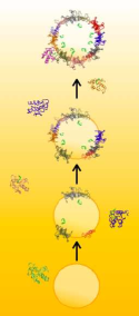
Figure 1: Foam forms in beer by the rising CO₂ bubbles that occurs as a result of the reduction in pressure on opening the container. Those rising bubbles collect surface-active materials, such as LTP1 and LTP1b, which form an elastic skin around the bubble to stabilize it. This figure is the schematic representation of the adsorption of LTP1 and LTP1b to the surface of beer foams. The ligand of LTP1b is colored green.

We focus on protein LTP1 (PDB:1LIP) and on LTP1b (PDB:3GSH) – its post-translationally modified isoform with a fatty ligand adduct. We do not consider protein Z because its native structure is not known. Proteins LTP1 and LTP1b are identical sequentially and their structures differ by 1.95 Å in RMSD (root-mean-square deviation) bakan2009 , which is a measure of the average distance between atoms in two superimposed conformations. As the reference conformation we take the crystal structure of the protein. We study what happens to the conformations of these proteins as they arrive at the air-water interface. The schematic representation of the adsorption of LTP1 and LTP1b to the surface of beer foams is shown in Fig. 1. These proteins form something like an elastic skin around a bubble and stabilize it. The ligand bound to LTP1b is ASY, which stands for $\alpha$-ketol, 9-hydroxy-10-oxo-12($Z$)-octadecenoic acid bakan2009 . The adduction process occurs during seed germination. The ligand is formed from linoleic acid by the concerted action of 9-lipoxygenase and allene oxide synthase bakan2009 . It is known that 1 kg of the barley seeds produces 103.3 and 82.7 mg of purified LTP1 and LTP1b proteins respectively jegou2000 .

Both isoforms contain four disulfide bonds when in barley seeds and in malt. These bonds form a cage delimiting the central hydrophobic cavity. In LTP1, the cavity is small but is capable of capturing different types of free lipids bakan2009 . On the other hand, in LTP1b, the cavity much bigger but is filled by about a half of the ASY ligand – the other half is outside of the protein. With the use of the spaceball server spaceball , we estimate that the volume of the cavity, $V_{c}$, is 69.192 and 666.488 ų for LTP1 and LTP1b (on removing the ligand) respectively. The sizes were determined by using a spherical probing particle of radius 1.42 Å, corresponding in size to the molecule of water. The cavity in LTP1b actually consists of three disjoint subcavities of comparable volumes. It appears that the process of adduction makes the protein looser and less rigid bakan2009 ; bettonigao . The near terminal regions move away from the center of the protein. It should be noted, however, that the structure of LTP1 has been determined through the NMR method and that of LTP1b by the X-ray crystallography.

During mashing, when hot water is added to malt to form wort (obtained after the removal of insoluble fractions during lautering), in which starches in barley are converted to sugars. At this stage, also the LTP1 and LTP1b proteins get glycated by forming covalent bonds with hexoses through the Maillard reaction jegou2001 . Glycation increases hydrophilicity and solubility of LTP1 isoforms and thus the foaming propensity jegou2000 without affecting the structural stability of the protein reppocheau .

In the next stage of beer production, wart boiling in the presence of a reducing agent such as sodium sulphite, the disulfide bonds get cleaved to varying degrees. The bigger the cleavage, the larger the probability for LTP1 and LTP1b to unfold irreversibly jegou2000 ; jegou2001 and thus to become better foam makers because the proteins flatten out wider at the interface and thus generate a more continuous protein layer. The native, compact isoforms display poor foaming properties bech1993 . However, this simple picture gets complicated in the presence of free lipids vannierop . These lipids destabilise beer foam by disrupting the adsorbed protein layers at the interface into foam lamellae clark1994 . This destabilisation is significantly reduced by the presence of LTP1s, as these proteins capture the lipids into their cavities and thus reduce the free lipid concentration. Thus, there should be an optimal degree of denaturation, at which LTP1s are unfolded at the interface sufficiently well to generate an increased surface coverage and yet are still able to bind free lipids. Interestingly, under the reducing conditions and in the presence of the lipids, LTP1b has been found to have a higher thermal stability than LTP1 by 15^∘C, as evidenced by the circular dichroism spectroscopyreppocheau .

In our theoretical model, we include the ASY, sugar ligands, and consider the proteins with various numbers, $n_{SS}$, of the disulfide bonds. The disulfide bonds may get reduced during malting and brewing. The reducing conditions are generated by malt extracts and also by yeastreppocheau . We study what happens to the ligands and the geometry of the proteins when they come to the interface. We show that the smaller the $n_{SS}$, the bigger the spreading of the proteins along the interface and thus larger stabilization of the foam. On the other hand, the thermal stability of the protein is expected to get reduced on lowering $n_{SS}$. Our discussion of the geometry also involves determination of the volume of the cavities that LTP1 and LTP1b turn out to be endowed with (we study the case of $n_{SS}$=4) and its dependence on the temperature, $T$.

It should be noted that the understanding of the properties of LTP1 is interesting beyond just beer making. This protein has been originally identified as promoting the transfer of lipids between donor and acceptor membranes in living plant cells carvalho . Its other physiological roles are not clear carvalho . However, LTP1 has been suggested to be important in the context of the response to changes in $T$ torres , drought connell , and bacterial and fungal pathogens michond . LTP1 is known to act as an allergen in plant food, such as fruits, vegetables, nuts and cereals, latex and pollens of parietaria, ragweed, olive, and mugwort salcedo2007 .

II Methods

In our coarse-grained model, we represent the LTP1 and LTP1b proteins by 91 effective atoms placed at the $\alpha$-C atoms. The interactions between the residues are described by the Lennard-Jones potential of depth $\varepsilon$, approximately equal to 110 pN Å or 1.6 kcal/mol. The value of $\varepsilon$ is estimated by benchmarking simulations to the experimental results on the characteristic unraveling force for 38 proteins in bulk water plos . This value is consistent with what was derived through all-atom simulations Poma . The length parameter, $\sigma$, is determined from the native distance between the residues. These interactions are assigned to native contacts, as determined through the overlaps (the OV contact map Wolek ) between atoms belonging to the residues. The cutoff of the Lennard-Jones potential is 20 Å. A contact is considered ruptured if the distance between the $\alpha$-Cs exceeds 1.5 $\sigma$. Pairs of residues that do not form a native contact interact through steric avoidance.

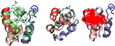
Figure 2: Left: Superimposition of the crystal structures of LTP1 (green) and LTP1b (the protein is color-ramped from red to blue, from the N- to the C-terminus). The carbons and oxygens of the ligand of LTP1b are shown in cyan and red beads. Middle: The placement of the four disulfide bonds in LTP1b. The eight cysteine residues involved in disulfide bonds are shown as black-yellow beads. The disulfide bonds in LTP1 connect the same sites as in LTP1b. Right: The three cavities in LTP1b (on removing the ligand) are indicated in red.

The four disulfide bonds connect cysteines at sites {3,50}, {13,27}, {28,73} and {48,87}, as illustrated in Fig. 2. They are described by the harmonic terms, similar to the tethering interactions in the backbone. Under the reducing conditions, some number of the disulfide bonds get cleaved and the properties of the resulting systems depend on the identity of the bonds that stay. For instance, there are 6 ways of removing two disulfide bonds. All possibilities are listed in Table 1, together with the notation used.

The backbone stiffness is described by a chirality potential Wolek1 . The solvent is implicit and is represented by the overdamped Langevin thermostat. Most of the molecular dynamics simulations are done at $T=0.3\;\varepsilon/k_{B}$ for which folding is optimal ($k_{B}$ is the Boltzmann constant); effectively, this corresponds to the room temperature. $T$ is controlled by introducing the implicit solvent as represented by the Langevin noise and damping terms in the equations of motion

$$m\ddot{\textbf{r}}=-\gamma\dot{\textbf{r}}+F_{c}+\Gamma\;\;.$$ (1)

Here, $F_{c}$ is the force due to all of the potentials that describe the protein and $m$ is the mass of the residue. We take the damping coefficient, $\gamma=\upsilon m/\tau$, where $\tau$ is a characteristic time scale. $\tau$ is of order 1 ns which reflects the diffusional instead of ballistic nature of the motion in the implicit solvent. The ballistic motion would correspond to the all-atom timescale of order ps. The factor of $\upsilon$ in the expression for $\gamma$ controlls the strength of damping. We have determined Hoang2 that $\upsilon\geq 2$ corresponds to overdamping when the inertial effects are minor. We take $\upsilon=2$ to have fast overdamped dynamics. $\Gamma$ is the random Gaussian force with dispersion $\sqrt{2\gamma k_{B}T}$ so that fluctuations are balanced by dissipation. The Langevin equations of motion are integrated by using the fifth order predictor-corrector scheme Tildesley .

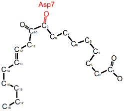
Figure 3: Schematic representation of the atomic structure of ligand ASY. The hydrogen atoms are not shown.

ASY consists of 18 carbon, 3 oxygen, and 32 hydrogen atoms. The 9th carbon C9 is covalently bound to the O2 atom of Asp 7 in protein LTP1b. The bonding site splits the ligand into two branches, see Fig. 3. In the native state, the branch extending from C1 to C8 lies on the hydrophobic surface of the protein, while the other branch is burried within the cavity as shown in Fig. 2 and 3. In the coarse-grained model, we represent ASY by 18 effective atoms located at the carbon atoms. The native contacts between the residues of LTP1b and ASY are determined by using the LPC/CSU server csu . There are 6 contacts that ASY makes with the outside part of the protein. These are: C1–Gly53, C2–Gly53, C4–Ile54, C5–Gly57, C6–Gly57 and C8–Ile54. In addition, there are 26 contacts within the cavity: C10–Asp7, C10–Lys11, C11–Asp7, C11–Lys11, C11–Ile54, C12–Lys11, C12–Leu14, C12–Ile58, C13–Met10, C13–Leu14, C13–Ile58, C14–Met10, C14–Ile54, C14–Ile58, C15–Met10, C15–Val17, C15–Ile58, C16–Met10, C16–Leu51, C17–Ile54, C17–Ala55, C17–Ile81, C18–Ala55, C18–Leu61, C18–Ala66 and C18–Ile81.

In our theoretical study, the presence of the air-water interface is simulated by an interface-related force that is coupled to the hydropathy index, $q_{i}$, of the $i$th residue airwater ; yani2016 . It is given by

$$F_{i}^{wa}=q_{i}\;A\;\frac{\text{exp}(-z_{i}^{2}/2W^{2})}{\sqrt{2\pi}W}$$ (2)

where $A$ is a measure of the strength of the force, $W$ is the width of the interface, and $z$ is the Cartesian coordinate that measures the distance away from the center of the interface. Generally, the negative values of $z$ correspond to water and positive to gas, but the transition between the two phases is gradual. The interface itself is in the $x-y$ plane. We use the values: $A$=10$\;\varepsilon$ and $W=5\;$Å. They were selected so that a protein arriving at the interface does not depart from it. The hydropathy indices are taken from ref. Kyte . They range from –4.5 for the polar arginine to 4.5 for the hydrophobic isoleucine. This scale is close to that derived by Wolfenden et al. Wolfenden as both scales have been derived from the physicochemical properties of amino acid side chains instead of from the probability of finding a residue in the protein core, as done in refs. Janin ; Rose . The force is acting on the hydrophilic residues points toward $z<0$ and on the hydrophobic ones toward $z>0$. The overall hydrophobicity for a protein of $N$ residues is given by $H\;=\;\frac{1}{N}\;\sum_{i=1}^{N}\;q_{i}$. For LTP1, $H$ is -0.38.

In the case of LTP1b, there is a need to define $q_{i}$ also for the atoms of the ligand. For this purpose, we use the non-overlaping molecular fragment approach clogp , abbreviated as ClogP. In this approach, one considers concentrations of a compound that is present in two coexisting equilibrium phases of a system and defines the partition coefficient as the ratio of these concentrations. It is assumed that the coefficient for the compound can be estimated as a sum of the coefficients of its non-overlapping molecular fragments. The fragments consist of a group of atoms and the neighboring fragments are assumed to be linked covalently. With the use of the BioByte’s Bio-Loom program biobyte we have determined that the hydrophilic head of ASY, consisting of C1 and two oxygen atoms (Fig. 3), can be assigned the ClogP value of –0.5. The tail C2–C18 is hydrophobic and each of the carbons in the tail has the ClogP value of 0.35. These ClogP values are taken the estimates of $q_{i}$. For alanine, this approach yields 1.1 which is close to the Kyte and Doolittle value of 1.8 Kyte . For LTP1b, we get $H=-0.27$.

II.1 Justification of the phenomenological model of the interface

In order to provide a qualitative atomic-level justification of the hydropathy-based model, we use the NAMD NAMD all-atom molecular dynamics package with the CHARMM22 force field charmm1 ; charmm2 and consider the following simulation set-up. The system is placed in a box which extends between –50 and +50 Å both in the $x$ and $y$ directions. In the $z$ direction, it extends between –90 and +90 Å. We situate the center of mass of LTP1 at point (0,0,0) and freeze the protein in its native state. We consider LTP1 with $n_{SS}$=4 and 0. There is a multitude of possible orientations that the protein can make. We select two which are defined with respect to the direction of the hydropathy vector airwater . This vector is defined as $\vec{h}=\frac{1}{N}\sum_{i=1}^{N}q_{i}\vec{\delta_{i}}$, where $\vec{\delta_{i}}$ is the position vector of the $i$th residue with respect to the center of mass of the protein. Orientation I corresponds to $\vec{h}$ pointing towards the positive $z$ axis. One of the hydrophobic residues at the top is leucine-61 and one of the hydrophilic residues at the bottom is glutamine-39. The distance between the $\alpha$-C atoms of these residues will be denoted by $d_{h}$. Orientation II is when $\vec{h}$ points in the opposite direction: leucine-61 is at the bottom and glutamine-39 at the top.

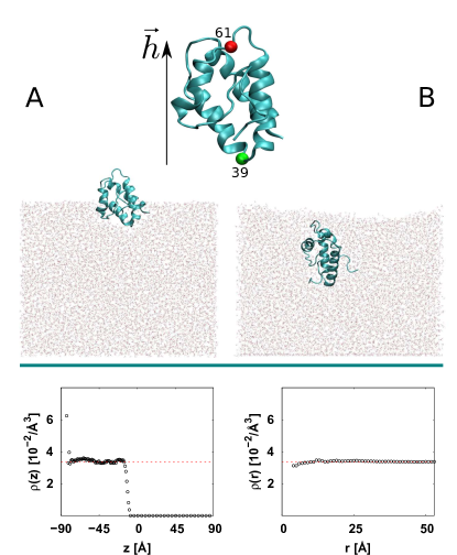
Figure 4: Top: Protein LTP1 in orientation I. The red sphere corresponds to the hydrophobic leucine-61 and the green sphere to the hydrophilic glutamine-39. Middle: The left panel shows the initial placement of the protein in water in orientatin I. The right panel shows LTP1 with $n_{SS}=4$ 12 ns later. A wall composed by asparagine residues is placed at the bottom of the system. The water molecules displayed are from the slice between $y$=–13 and 20 Å (the $y$ direction is perpendicular to the plane of the figure). Bottom: The number density profiles of the air-water system along $z$-axis and the radial direction in the $x-y$ plane. The red dashed line indicates the level characterizing water under atmospheric pressure.

We then place 26 381 molecules of water, as described by the TIP3P model water , in the space corresponding to $z\leq 0$ and outside of the region occupied by the protein. Two Cl^- ions are added to the solvent to neutralize the charge of LTP1. We do not build a specific ionic strength because it is not clear what it should be. In order for the water molecules to prefer staying in the lower half of the simulation box, we set a hydrophilic wall at $z$=–90 Å. The wall is made of a single layer of 6728 asparagines (see panel A of Fig. 4). The $\alpha$-C atoms of the asparagines ($q_{i}$ of -3.6) are anchored to the sites of the [001] face of the fcc lattice with the lattice constant of 5 Å. The side groups of the residues are directed towards water and they stay frozen. We use periodic boundary conditions and the Particle Mesh Ewald method Darden .

The system of the water molecules is then equilibrated at $T=$300 K for 2 ns. The number density profile of the water molecules along $z-$ and the radial direction in the $x-y$ plane is shown in the bottom panels of Fig. 4. The results are time-averaged over 5 ns based on frames as obtained every 20 ps with the protein staying frozen. The density profile $\rho(r)$ in the $x-y$ plane is averaged over all values of $z$ except for the immediate vicinity of the bottom wall. It is calculated starting from $r=5$ Å to avoid the excluding effects of the protein. The attractive wall pulls water in and sets the number density of water at $3.37\pm 0.60\times 10^{28}$ m^-3 which is consistent with $3.34\times 10^{28}$ m^-3 for water under normal conditions. We observe that $\rho(z)$ goes down from the bulk value to zero at $z=-5$ Å and the width of the interface is about 8 Å. The radial distribution function, averaged over the regions of bulk water, is nearly constant.

We now unfreeze the protein and equilibrate the whole system in two steps: 2 ns at $T$=150 K and 10 ns at 300 K. The protein is overall hydrophilic so it gets drowned in water, as shown in panel B of Fig. 4 for the case of $n_{SS}=4$, but it stays at the interface for about 11 ns. The water coverage in the panel is shown in an exaggerated way because all molecules in the system are projected into the $x-z$ plane.

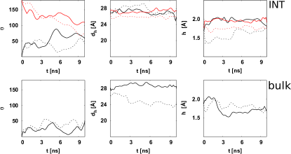
Figure 5: Comparison of the behavior of the protein at the interface and in the bulk water as characterized by $\theta$, $d_{h}$, and $h$. The black lines are for orientation I: solid line for $n_{SS}$=4 and the dashed line for $n_{SS}$=0. The red lines are for orientation II with the similar convention regarding the value of $n_{SS}$. In the bulk situation, the initial orientation is selected randomly.

We monitor the orientation and the change in shape of the protein in the time interval in which it is pinned at the interface. One parameter is $\theta$ - the angle that the vector $\vec{h}$ makes with the $z$-axis. Initially it is 0 for orientation I and 180 for orientation II. In bulk water, $\theta$ is measured with respect to the initial random orientation. At the interface, orientation I should favor not making any major change in $\theta$. Instead, it evolves to about 70^∘, as shown in the left panels of Fig. 5. The reason is that the force field we use is not fully compatible with the hydropathy indices – the indices have not been obtained through molecular dynamics calculations. We observe that when one starts with the 70^∘ orientation then the protein just fluctuates around it for as long as it stays at the interface, indicating a compatibility with the hydropathy related forces. Thus molecular dynamics may provide a way to rederive hydropathy indices. For orientation II, it is expected that $\theta$ would merge with the range of values obtained for orientation I if it could stay at the interface longer.

In order to monitor the changes in the shape, we consider $d_{h}$ and $h=|\vec{h}|$. For $n_{SS}$=4 both parameters are close to that obtained in bulk water (the middle and right panels in Fig. 5). However, for $n_{SS}$=0 both parameters indicate an expansion compared to the bulk situation. We conclude that the atomic-level considerations support the orientational and conformational effects produced by the phenomenological model described by Eq. (2). Events of the interface depinning (often followed by events of repinning) can by captured by a reduction in the value of $A$. However, our test runs do not indicate any depinning for several other proteins. Other force-fields may extend the time at the interface for LTP1. We work in the limit in which no depinning is expected.

III Results

III.1 Properties of single proteins away from the interface

We characterize the equilibrium properties of the proteins by three quantities: $P_{0}$, $Q$, and the root mean square fluctuation (RMSF), which is a measure of positional fluctuations of a residue with respect to its initial location. These quantities are determined based on 5 long runs (100 000 $\tau$ each) that start in the native state and correspond to a temperature $T$. The first of these is the probability of all native contacts being present simultaneusly. The disulfide bonds do not count as contacts. The temperature, $T_{0}$, at which $P_{0}$ crosses through $\frac{1}{2}$ is a measure of the melting temperature. $Q$, on the other hand, is a fraction of the native contacts that are established (i.e. without the condition of the simultaneous presence of all contacts). The temperature, $T_{Q}$, at which $Q$ crosses through $\frac{1}{2}$ is close to a maximum in the specific heat which signifies a transition between extended and globular conformations. This point is discussed further in ref. Wolek1 . $T_{Q}$ is necessarily much higher than $T_{0}$. $P_{0}$ and $Q$ provide global characterization whereas RMSF give local information about the magnitude of the positional fluctuations of the $i$th residue.

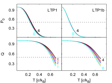
Figure 6: The temperature dependence of $P_{0}$ and $Q$ for LTP1 (left) and LTP1b (right) in bulk water for the indicated values of $n_{SS}$. The data points are averaged over all possible permutations of the disulfide-bond placement. The dashed lines correspond to the level of $\frac{1}{2}$.

Fig. 6 shows the $T$-dependence of $P_{0}$ and $Q$ for LTP1 for various values of $n_{SS}$. The data is averaged over the permutations. The values of $T_{0}$ do not vary much: it is 0.257 $\varepsilon/k_{B}$ for $n_{SS}$=4 and 0.236 $\varepsilon/k_{B}$ for $n_{SS}$=0 – less than 1^∘C difference. At $T$=0.5$\;\varepsilon/k_{B}$, i.e. at about 100^∘C, the differences in $Q$ remain small, indicating a remarkable thermal stability. Our observations agree with the results in ref. larsen2001 that there is no major structural change in LTP1 taking place between 20 to 90^∘C. For LTP1b, the ligand related contacts are counted in the calculation of $P_{0}$ and $Q$. These contacts are easy to rupture on heating, which results in LTP1b being a less stable structure than LTP1.

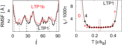
Figure 7: Left: RMSF of LTP1 (black lines) and LTP1b (dotted red lines) in bulk at $T=0.5\varepsilon/k_{B}$ and for $n_{SS}=0$. The RMSF of the eight cysteine residues involved in the formation of disulfide bonds are indicated by the dashed vertical lines. Right: The temperature dependence of the median folding time, $t_{f}$, for LTP1 with $n_{SS}$ equal to 4 (the black line) and 0 (the red line).

Fig. 7 (the right panel) shows the $T$-dependence of the median folding time, $t_{f}$, for LTP1 at $n_{SS}$=4 and 1. $t_{f}$ is calculated by considering 100 trajectories which start from a conformation without any contacts and by determining the median time needed to establish all native contacts for the first time. The dependence is U-shaped and the center of the U defines the temperature of optimal folding, $T_{min}$. We get $T_{min}$ of 0.26 and 0.24 $\varepsilon/k_{B}$ for $n_{SS}$ of 4 and 0 respectively, indicating an overall leftward shift. The basins of good folding are rather broad and $T_{0}$ is within the basins.

Fig. 7 (the left panel) compares the RMSF for LTP1 and LTP1b at $n_{SS}$=0. In order to enhance the difference between the patterns, the comparison is done at $T$=0.5 $\varepsilon/k_{B}$. The presence of the ligand is seen to increase the fluctuations at almost all sites. The cysteine residues have varying levels of the RMSF. We find that if a disulfide bond was replaced by a regular contact then the most fragile of them is 3–50, and the most persistent is 48–87 (for LTP1, the probability of the contact being present is 56% and 65% respectively; $T$=0.5 $\varepsilon/k_{B}$). There are two reasons for the fragility of the 3–50 contact. First, residue 3 is close to the terminus. Second, the contact has the largest contact order, as measured by the sequential distance between the residues. We conclude that, for both proteins, the 3–50 disulfide bond is the most likely to be cleaved and 48-87 is the least likely. Experimentally, one can study the reduction of disulfide bonds through titration with DTNB (5,5’-Dithiobis-(2-nitrobenzoic acid) or Ellman’s reagent), which reacts with sulfhydryl groups jegou2000 . This method provides a reliable way to measure the concentration of the reduced cysteines but it does not indicate the persistence levels of specific bonds.

III.2 Properties of single proteins at the interface

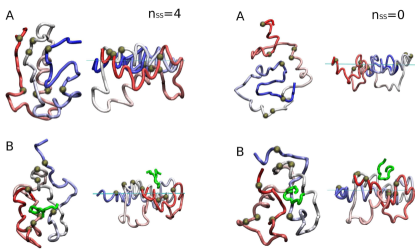
Figure 8: Left: The top and side view of the most probable conformation of LTP1 (A) and LTP1b (B) at the air-water interface at $T=0.3\varepsilon/k_{B}$ with $n_{SS}=4$. The 8 cysteines involved in disulfide bonds are shown in black-yellow beads and the ligand of LTP1b is shown in green. Right: The same as the left panel but for $n_{SS}=0$. The N-terminus of proteins is showed in red and the C-terminus is in blue.

When studying the effects of the interface, we delimit the space by repulsive walls at $z$=-10 nm and $z$=10 nm and place the protein close to the bottom wall, but still in ”bulk water”. We then evolve the system for 10 000 $\tau$ to allow the protein to come to the interface and to adjust to it. The interface deforms the protein, as illustrated in Fig. 8 for LTP1, because of the hydropathy-related forces. In particular, we observe the collapse of the cavity. In the case of LTP1b, the collapse is concurrent with the expulsion of the ASY tails toward the gas phase.

In order to characterize the deformed geometry, we define three parameters: $R_{z}$, $d_{z}$, and $w$. The first of these is the radius of gyration in the $x-y$ plane, $R_{z}=\{\frac{1}{2N^{2}}\sum_{i,j}\left[(x_{i}-x_{j})^{2}+(y_{i}-y_{j})^{2}\right]\}^{\frac{1}{2}}$, where $x_{i}$, $x_{j}$, $y_{i}$ and $y_{j}$ are the $x$ and $y$ coordinates of the $i$ and $j$th residues. The second parameter is the vertical thickness of the protein, defined as the extension along the $z$-axis. The third parameter describes the nature of the shape of the protein. It is defined as $w=\Delta R/\bar{R}$ with $\Delta R=R_{2}-\bar{R}$ and $\bar{R}=1/2*(R_{1}+R_{3})$. $R_{1}$, $R_{2}$, and $R_{3}$ are the main radii of gyration, derived from the moment of inertia, and ranked ordered from the smallest to the largest. $w\approx 0$ corresponds to a globular shape, $w<0$ to a flattened conformation, and $w>0$ to an elongated one. In the case of LTP1b, the ligand is taken into account in the calculation of the geometrical parameters. When comparing a parameter $X$ (like $R_{z}$) between the two proteins, we take LTP1 to be the reference system and define the relative difference by $r_{X}=(X_{\text{LTP1b}}-X_{\text{LTP1}})/|X_{\text{LTP1}}|$.

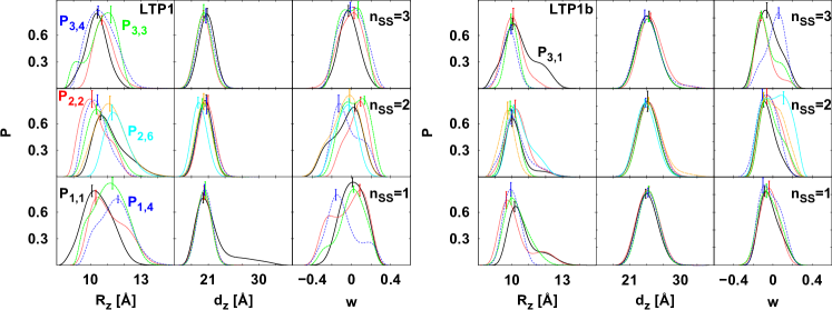
Figure 9: The normalized histogram of $R_{z}$, $d_{z}$ and $w$ for LTP1 (left) and LTP1b (right) at the interface at $T=0.3\varepsilon/k_{B}$. The values of $n_{SS}$ range between 1 and 3. In this plot, the permutation $P_{3,1}$, $P_{2,1}$ and $P_{1,1}$ are in black, $P_{3,2}$, $P_{2,2}$ and $P_{1,2}$ in red, $P_{3,3}$, $P_{2,3}$ and $P_{1,3}$ in green, $P_{3,4}$, $P_{2,4}$ and $P_{1,4}$ in blue, $P_{2,5}$ in orange, and $P_{2,6}$ in cyan.

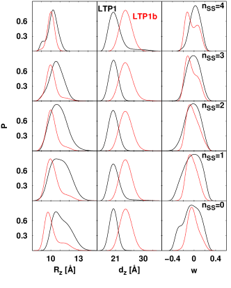
Figure 10: The normalized histogram of $R_{z}$, $d_{z}$ and $w$ for LTP1 (black) and LTP1b (red) at the interface at $T=0.3\varepsilon/k_{B}$. Tha data is for all possible values of $n_{SS}$ and for all allowed permutations.

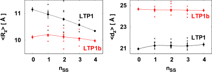
Figure 11: $\langle R_{z}\rangle$ and $\langle d_{z}\rangle$ for LTP1 (black circles) and LTP1b (red diamonds) at $T=0.3\varepsilon/k_{B}$ as a function of $n_{SS}$. For $1\leq n_{SS}\leq 3$, the data of each permutation is displayed as crosses. The errors of the means have been obtained by considering 50, 80, 120, 80 and 50 trajectories for $n_{SS}$ between 0 and 4 respectively and by partitioning the data into groups.

We generate 10 trajectories of coming to the interface analyze the conformations obtained at a permutation of $n_{SS}$. Each trajectory lasts for 100 000 $\tau$ and we store the conformations obtained every 15 $\tau$ (1$\tau$ corresponds to 200 integration steps). In the analysis, we take into account only those conformations in which the protein is at the interface. Figs. 9 and 10 show the normalized histograms of $R_{z}$, $d_{z}$ and $w$ of partially reduced LTP1 and LTP1b at various stages of the disulfide-bond reduction. Fig. 9 distinguishes between the permutations of the bond placement, if more than one is possible, whereas Fig. 10 shows the distributions that are averaged over the permutations. Table 2 summarizes the results by averaging over the distributions. Another summary is presented in Fig. 11, where the average values of $R_{z}$ and $d_{z}$, with the division into the permutations and without, are plotted vs. $n_{SS}$.

Generally, the smaller the $n_{SS}$ the bigger the spread of the proteins in the $x-y$ plane. One might expect that this effect should be coupled to the narrower the vertical extension, but this is not necessarily so: the dependence on the permutation dominates. The average value of $w$ is close to zero but the spread in this parameter is significant: between –0.4 and +0.4, indicating a large variation in the shapes of the conformations.

We also observe a substantial sensitivity in the geometrical parameters to the choice of the permutation. For example, at $n_{SS}=2$, the most probable value (the highest peak in the histogram in Fig. 9) of $R_{z}$ for LTP1 is at 10.04 Å and it is observed for permutation $P_{2,2}$. On the other hand, for permutation $P_{2,6}$ it is at 11.14 Å. For $n_{SS}=1$, the difference between the most probable values of $R_{z}$s is about 1.6 Å – it is smaller for $P_{1,1}$ than for $P_{1,4}$. The reason is that permutations $P_{2,2}$ and $P_{1,1}$ contain disulfide bond $\{3,50\}$ but exclude $\{48,87\}$, while $P_{2,6}$ and $P_{1,4}$ do the opposite. The disulfide bond $\{3,50\}$ involves sites that would fluctuate more vigorously than $\{48,87\}$ if the bonds were broken. Thus permutations $P_{2,2}$ and $P_{1,1}$ limit the fluctuations in the protein maximally, which leads to smaller values of $R_{z}$, than the other permutations.

In the case of LTP1b, the differences between various permutations are smaller than for LTP1. The reason is that the dominant shape-changing effect is due to the hydrophobic ligand which induces stretching which is more vertical and comes with generally smaller values of $R_{z}$.

The distributions shown in Figs. 9 and 10 are mostly Gaussian but some display shoulders. The shoulders reflect existence of various modes of the arrival at the interface and, therefore, of different modes of action of the hydropathy-related forces. Examples of the conformations show in Fig. 8 for $n_{SS}=4$ and 0 correspond to the dominant peaks in the distributions.

Fig. 11 illustrates our observation that $<R_{z}>$ and, therefore, the surface area of LTP1 and LTP1b increases as more disulfide bonds are cleaved. Moreover, the surface area of LTP1 is bigger than that of LTP1b for any value of $n_{SS}$ due to the vertical dragging action of the ligand in LTP1b. Also, $<d_{z}>$ is by about 3 Å larger for LTP1b than for LTP1. We conclude that the reduced LTP1 protein is a better surfactant as it spreads more and thus lowers the surface tension of foam. However, LTP1b contributes to a better adsorption at the interface, packs better. Both kinds of proteins are present in the foam and the two effects coexist.

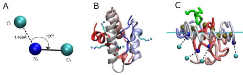
Figure 12: A: Schematic representation of the C-N covalent bond (dotted line) formed between the C₁ atom of glucose and the nitrogen N_ξ from the side chain of lysine. The bond length is 1.469 Å, and the angle made by C₁, N_ξ and the connected C_ε is 120^∘. B: Four glucoses (cyan) are covalently bound to four lysine residues of LTP1b (the ASY ligand is not displayed). The N-terminal part of the protein is shown in red and the C-terminal in blue. C: The location of glucoses bound to LTP1b at the interface. The glucoses and the lysine residues are shown as cyan and blue beads, respectively. The color coding of the terminal parts are as in panel B. The 8 cysteines shown in dark-yellow beads and the ligand ASY is shown in green.

We now consider the role of glycation. It has been arguedjegou2000 that glycation involves the nitrogens either from the N-terminus or from the nucleophilic amino group on the side chain of lysine residues. It results in formation of the C-N covalent linkage between the carbonyl group of sugars. Since the nitrogens on the side chains, denoted by N_ξ, are more exposed in solution, we focus only on the glycation on lysins. Concentration-wise, glucose and sucrose are the top two sugars in barley after germination allosio2000 . There are four lysins in LTP1 and LTP1b – they can bind to four sugar molecules each. Here, we consider the case of glucose. The geometry of binding is illustrated in Fig. 12.

In our coarse-grained model, each glycated glucose is represented as an effective atom. The bond length of the C-N covalent bond is taken as 1.469 Å, bondl and the bond angle as 120^∘. The rotation angle is taken randomly. The predicted ClogP value for a glucose is -2.21 which signifies that it is hydrophilic. As a result, glucoses at the interface point toward bulk water, as illustrated in Fig. 12, panel C.

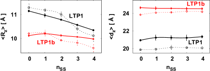
Figure 13: The comparison of $<R_{z}>$ and $<d_{z}>$ between the glycated (empty data points) and non-glycated (full data points) LTP1 and LTP1b for the 5 values of $n_{SS}$. The results are averaged over the permutations in the placement of the disulfide bonds. The error bars have been estimated as in Fig. 11.

Fig. 13 shows that glycation affects $<R_{z}>$ in a way that depends on the level of reduction. For $n_{SS}$ equal to 0 or 1, the surface area is enhanced for LTP1, but is about the same for LTP1b. For $n_{SS}$ of 2, it is enhanced for LTP1 but decreased for LTP1b. For $n_{SS}$ of 3 or 4, it is decreased for both proteins. The vertical spread $<d_{z}>$ is reduced on glycation in all cases. We conclude that, at high levels of reduction, glycation should enhance foam making by LTP1, but not by LTP1b. In beer, LTP1 and LTP1b coexist and the overall surface activity of the system is thus enhanced, in agreement with ref. jegou2001 .

III.3 Protein layers at the interface

In order to study protein layers, we need to define the interactions between individual proteins. In the simplest model, one takes only the excluded volume effects into account. A better model augments this description by introducing some attractive inter-protein contacts. Here, we do it in a different way than described in ref. airwater , where the selection of possible interactions was based on the consideration of the native contact map of one protein. Instead, we couple two hydrophobic residues, at site $i$ on one protein and at site $j^{\prime}$ on another, whenever the distance between their $\alpha$-C atoms is smaller than 12 Å. We describe the coupling by the Lennard-Jones potential in which the energy parameter is given by $\lambda\;\varepsilon$. If $\lambda=1$ then the depth of the potential well is the same as for the intra-protein contacts; if $\lambda=0$ then only the steric repulsion is involved. The length parameter, $\sigma^{\prime}$, is set to $(R_{\alpha C,i}+R_{\alpha C,j^{\prime}})/2$. Here, $R_{\alpha C,i}$ denotes the most likely radius of an effective sphere that can be associated with the $i$th residue when it forms the overlap-based contact that involves the residue. The values of $R_{\alpha C,i}$ are residue-specific and are listed in ref. mcpoma .

Another change is that we augment the single-protein simulational geometry by introducing a repulsive square box in the $x-y$ plane. We release $N_{p}$ identical proteins simultaneously, at random $x$, $y$ locations near the bottom. The lateral size, $l$, of the box determines the 2-dimensional number density, $n_{2}$ of the proteins that arrive at the interface and stay there diffusing. We consider $N_{p}$ of either 20 or 40 and $l$ that is initially set to 2000 nm and then adiabatically changed to 10 nm within 10 000 $\tau$. The system is then evolved for an additional 100 000 $\tau$. The time scale of the simulations has been chosen based on our previous studies of protein G and lysozyme airwater . $N_{f}$ of the $N_{p}$ proteins form a layer at the interface. The remaining proteins cannot squeeze in and are found in the second and higher order layers.

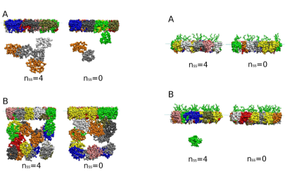
Figure 14: Examples of conformations obtained at the air-water interface for $N_{p}$ proteins with $\lambda=0$ – the side views. The left half of the figure is for the LTP1 molecules and the right half – for the LTP1b molecules (the ligands are in green). The left panels in each half are for $n_{SS}$ of 4 and the right panels for $n_{SS}$ of 0. The upper half of the figure is for $N_{p}$ of 20 and the lower half for $N_{p}$ of 40. The corresponding numbers of the proteins in the first layer are listed in Table 3.

We first consider the case of $\lambda=0$. Table 3 gives the values of $N_{f}$ in the case of $N_{p}=20$ and 40 at $T=0.3\varepsilon/k_{B}$. The proteins are either of one kind or mixed evenly – the situation referred to as mixed. We consider only the cases of $n_{SS}$=4 and 0. The table indicates that $N_{f}$ is larger for LTP1b than for LTP1, irrespective of the number of the disulfide bonds. The smaller surface area that characterizes LTP1b at the interface allows for more molecules to be placed at the first layer, as illustrated in Fig. 14. Moreover, the ligand adduct of LTP1b contributes to a better interface adsorption compared to LTP1. As a result, $n_{2}$ in the case of LTP1b is 0.20 nm^-2 for $N_{p}=20$ and for the two considered values of $n_{SS}$, while in the case of LTP1 it is 0.15 or 0.17 nm^-2 depending on whether $n_{SS}$ is 4 or 0. In the mixed case with $N_{p}=20$, all LTP1b molecules are adsorbed in the first layer while some LTP1 are found in the second layer ($n_{2}$ is 0.18 ($n_{SS}=4$) or 0.19 nm^-2 ($n_{SS}=0$)). All of this data indicates that LTP1b leads to denser protein layers.

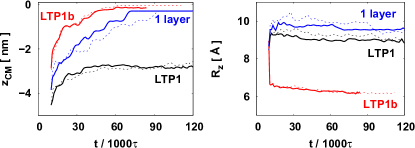
Figure 15: The time evolution of the average $z_{CM}$ and $R_{z}$ for LTP1 (the black lines) and LTP1b (the red lines) in the case of $N_{p}$=40 with $\lambda=0$. The solid lines correspond to $n_{SS}=4$ and the dashed lines to $n_{SS}=0$. The blue lines, labelled with ”1 layer”, correspond to the situation in which all LTP1 proteins arrange into just one layer: $N_{p}=15$ for $n_{SS}=4$ and 17 for $n_{SS}=0$.

Fig. 15 illustrates the dynamics of the proteins coming to the interface for $N_{p}$=40 ($\lambda=0$). The left panel shows the time dependence of the average center of mass in the $z$ direction, $z_{CM}$. The right panel shows the time dependence of the average $R_{z}$. It appears that the changes in the geometry take place faster than the progression toward the surface. The rate of progression is not sensitive to the value of $n_{SS}$.

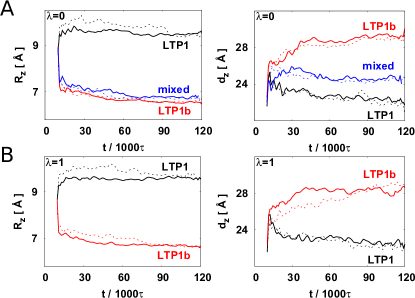
Figure 16: A: The time evolution of the average $R_{z}$ and $d_{z}$ for LTP1 (the black lines), LTP1b (the red lines) and their mixture (the blue lines) in the case of $N_{p}$=20 with $\lambda=0$. The solid lines correspond to $n_{SS}=4$ and the dashed lines to $n_{SS}=0$. B: The same as A but for $\lambda=1$.

The time-dependence of the shape parameters $R_{z}$ and $d_{z}$ for the LTP1, LTP1b and the mixed systems of $N_{p}=20$ is shown in Fig. 16 for $n_{SS}$ of 0 and 4. For $\lambda=0$, $R_{z}$ of the mixed case is much closer to that of LTP1b than LTP1, while $d_{z}$ is in between. (The corresponding $R_{z}$ is about 30% smaller for LTP1 but about 3% larger than for LTP1b; $d_{z}$ is 9% larger than for LTP1 but 13% smaller than for LTP1b).

Fig. 16 (panels B) also addresses the situation with $\lambda=1$. We observe that the effect of the attractive contacts on the shape parameters is minor – smaller than that associated with the variations in $n_{SS}$. For LTP1, at the end of the time evolution, $R_{z,\lambda=0,n_{SS}=4}$ is 0.4% smaller than $R_{z,\lambda=1,n_{SS}=4}$ and 2.5% smaller than $R_{z,\lambda=0,n_{SS}=0}$. Also, $d_{z,\lambda=0,n_{SS}=4}$ of LTP1 is 0.9% larger than $d_{z,\lambda=1,n_{SS}=4}$ and 0.7% larger than $d_{z,\lambda=0,n_{SS}=0}$. Similar results are also obtained for LTP1b.

III.4 The temperature dependence of the size of the cavity

One problem arising when determining the volume of a protein cavity, which is exposed to the solvent, is how to decide about its closure. We avoid making such decisions by using the spaceball algorithm spaceball which relies on the statistical analysis of the volume calculations obtained for various rotated grid orientations with respect to the protein. We surround the protein by a rectangular box and generate a grid of points through intersections of lines that are parallel to the box edges. The lines are taken to be separated by 0.2 Å. We then take spherical molecular probes (of radius 1.42 Å) and ”walk” them along the three lattice directions until they encounter an atom of the protein or the opposite wall. The van der Waals radii of the atoms are taken from ref. Tsai . The sites that have not been visited define the cavity space for this particular orientation. We then consider 25 rotations to change the orientation and average the results. The average defines the most typical (as opposed to extremal) value of the volume. As mentioned in the Introduction, this method yields $V_{c}$ of 69.192 and 666.488 ų for LTP1 and LTP1b (with the removed ligand) respectively, if one uses the PDB structure files. In the case of LTP1, there are two disconnected cavities of 43.384 and 25.808 ų. In the case of LTP1b – three of 262.784, 212.616, and 191.088 ų.

It should be noted that different estimates have been obtained with the use of the VOIDOO program voidoo : no cavity in the case of LTP1 and two cavities of 548 and 568 ų in the case of LTP1b bakan2009 . In this program, one first identifies the outside surface of the protein and then sets a grid of lattice points that are surrounded by this surface. One considers one orientation of the grid and the grid spacing is set between 0.5 and 1.0 Å. In order to take into account the excluded volume effects, one uses a probe of radius 1.4 Å. The grid points are all initialised to count as 0. This value is turned to 1 if the grid point distance to the closest protein atom is smaller than the sum of the probe radius and the van der Waals radius associated with the atom. All grid points with the 0 value are away from the cavity wall and thus count as contributing to the volume of the cavity. In this procedure, the opening of the cavity is typically ill-defined and one alleviates the problem by enlarging, or ”fattening”, the van der Waals radii by a factor until the cavity gets closed. The VOIDOO program gives larger volumes than the procedure used by us because the opening of the cavity counts too much even with the fattening procedure. We consider our procedure to be more accurate because our grid size is smaller and because the enlargment of the radii to define the closure of the cavity introduces errors also away from the closure. We have made an independent check of the cavity geometry by indentifying the atoms on the inside of the cavity and determining distances between them. By doing so we could determine that LTP1 and LTP1b can accomodate about 3 and 7 water molecules respectively.

It is interesting to find out how does $V_{c}$ depend on $T$. We use the NAMD all-atom molecular dynamics package NAMD with the CHARMM22 charmm1 force field to generate conformations corresponding to a given $T$ and apply the spaceball algorithm to a sample of conformations. The ASY ligand is removed from LTP1b. The system is equilibrated for 2 ns, in which time the temperature is increased in three steps from 110K, to 210K, and to the final $T$ (of 250K, 300K, 325K, 350K, 375K and 400K). For $T\leq 200$K, the system is equilibrated in one step. We pick 10 conformations for further analysis.

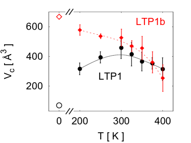
Figure 17: The comparison of the cavity volume $V_{c}$ of LTP1 (black) and LTP1b (red, after removing the ligand) at different temperatures. The data for $T=0$ K (the empty symbols) correponds to the native state of the protein. All protein conformations are obtained from NAMD all-atom simulation in case of $n_{SS}=4$.

Fig. 17 shows the estimated $V_{c}$ for LTP1 and LTP1b as a function of $T$. For LTP1b, $V_{c}$ is seen to decrease monotonically as $T$ increases. This is because the stronger thermal fluctuations limit the free space inside of the protein. For LTP1, $V_{c}$ increases from 69.192 ų (see the empty black circle in Fig. 17) in the native state to 457.564 ų at $T$=300K, then drops down monotonically as $T$ increases still further. The difference in behavior between LTP1b and LTP1 stems from the fact that LTP1b is loosely packed, especially after removing the ligand, whereas LTP1 is tightly packed. As $T$ increases, LTP1 gets partially unfolded which makes the protein swallen and endowed with a bigger cavity. However, on a further increase in $T$, the thermal fluctuations reduce the effective volume of the cavity. For LTP1b, it is only the thermal fluctuations that affect the volume of the cavity. We observe that even though $V_{c}$ for LTP1b is larger than for LTP1 at room $T$, the volumes become more and more alike as $T$ grows. This is because of the smaller rigidity of LTP1b, as evidenced in Fig. 7.

IV Conclusions

We have used the structure-based coarse-grained model to elucidate the nature of the conformational transformations of LTP1 and LTP1b at the air-water interface in the context of beer foaming. We have constructed an all-atom model that supports the basics of the phenomenological description of the interface used in the coarse-grained model. Though our results are of a fairly qualitative nature, they provide molecular-level insights into the process. Both of these proteins are shown to deform and span the interface to stabilize it. The degree of spreading depends on the number of the disulfide bonds: the smaller this number, the larger the surface area covered (see Fig. 11). We find that LTP1 spreads more than LTP1b because of the fatty ligand. The ligand makes the protein layer to be more packed and thicker. The increased thickness should contribute to a slower flow rate of liquid drainage of beer foams observed by Bamforth et al. evan2009 . We also show that glycation increases the surface area at sufficiently high levels of the disulfide-bond reduction. We have argued that the {3,50} disulfide bond is more likely to be cleaved than {48,87} and that the structural properties of the proteins at the interface depend on which bonds are actually cleaved. We have provided new estimates of the volumes of the cavities in the two proteins and showed that the volumes generally decrease on heating. Thus heating should lead to a smaller propensity to bind free lipids.

Acknowledgements

We appreciate fruitful discussions with G. Rose and A. Sienkiewicz as well the technical help from M. Chwastyk. The project has been supported by the National Science Centre (Poland), Grant No. 2014/15/B/ST3/01905, European Framework Programme VII NMP grant 604530-2 (CellulosomePlus).

Table 1: The list of possibilities of having the disulfide bonds in LTP1 and LTP1b under the conditions of various levels of reduction as characterized by $0\leq n_{SS}\leq 4$. For $1\leq n_{SS}\leq 3$, the permutations are denoted by $P_{n_{SS},{\lambda}}$ where $\lambda$ varies between 1 and 6 if $n_{SS}$=2 or between 1 and 4 if $n_{SS}$ is either 1 or 3.

$n_{SS}$	number of permutation	list of permutations $P_{n_{SS},{\lambda}}$
4	1	{3,50} {13,27} {28,73} {48,87}
3	4	$P_{3,1}$: {3,50} {13,27} {28,73} $P_{3,2}$: {3,50} {13,27} {48,87} $P_{3,3}$: {3,50} {28,73} {48,87} $P_{3,4}$: {13,27} {28,73} {48,87}
2	6	$P_{2,1}$: {3,50} {13,27} $P_{2,2}$: {3,50} {28,73} $P_{2,3}$: {3,50} {48,87} $P_{2,4}$: {13,27} {28,73} $P_{2,5}$: {13,27} {48,87} $P_{2,6}$: {28,73} {48,87}
1	4	$P_{1,1}$: {3,50} $P_{1,2}$: {13,27} $P_{1,3}$: {28,73} $P_{1,4}$: {48,87}
0	1	–

Table 2: The average values of $R_{z}$, $d_{z}$ and $w$ for LTP1 and LTP1b, together with their relative differences, as a function of $n_{SS}$ at $T=0.3\varepsilon/k_{B}$. For $n_{SS}=4$ or 0, the data is averaged over 20 trajectories. For $1\leq n_{SS}\leq 3$, we have generated 10 trajectories for each permutation.

$n_{SS}$	LTP1			LTP1b			$r_{\langle R_{z}\rangle}$	$r_{\langle d_{z}\rangle}$	$r_{\langle w\rangle}$
	$\langle R_{z}\rangle$ Å	$\langle d_{z}\rangle$ Å	$\langle w\rangle$	$\langle R_{z}\rangle$ Å	$\langle d_{z}\rangle$ Å	$\langle w\rangle$
4	10.15	21.35	+0.02	9.98	24.54	-0.04	-1.7%	14.9%	-30.0%
3	10.57	21.23	-0.01	10.07	24.55	-0.05	-4.7%	15.6%	-40.0%
2	10.79	21.24	-0.03	10.13	24.57	-0.02	-6.1%	15.7%	33.0%
1	10.97	21.25	-0.03	10.20	24.59	-0.04	-7.0%	15.7%	-33.0%
0	11.15	20.94	-0.05	10.12	24.65	-0.02	-9.2%	17.7%	60.0%

Table 3: The number of adsorbed molecules $N_{f}$ in the first layer for the total number of $N_{p}$ proteins for $\lambda=0$ and for a given value of $n_{SS}$. The term mixed refers to a situation in which 50% of the proteins are LTP1 and the other 50% are LTP1b.

protein	$N_{f}$ ($N_{p}=20$)		$N_{f}$ ($N_{p}=40$)
	$n_{SS}=4$	$n_{SS}=0$	$n_{SS}=4$	$n_{SS}=0$
LTP1	15	17	21	22
LTP1b	20	20	39	40
mixed	18	19	–	–

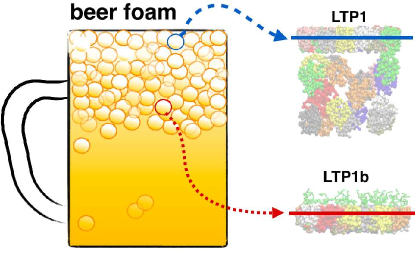
Figure 18: The table of contents (TOC) graphic.

References

- (1) Bhakta, S. A.; Evans, E.; Benavidez, T. E.; Garcia, C. D. Protein adsorption onto nanomaterials for the development of biosensors and analytical devices: A review. Anal. Chim. Acta 2015, 872, 7-25.
- (2) Nawrocki, G.; Cieplak, M. Aqueous Amino Acids and Proteins Near the Surface of Gold in Hydrophilic and Hydrophobic Force Fields. J. Phys. Chem. C 2014, 118, 12929-12943.
- (3) Nawrocki, G.; Cazade, P.-A.; Thompson, D.; Cieplak, M. Peptide recognition capabilities of cellulose in molecular dynamics simulations. J. Phys. Chem. C 2015, 119, 24402-24416.
- (4) Sengupta, T.; Damodaran, S. Role of dispersion interactions in the adsorption of proteins at oil-water and air-water interfaces. Langmuir 1998, 14, 6457-6496.
- (5) Leiske, D. L.; Shieh, I. C.; Tse, M. L. A method to measure protein unfolding at an air-liquid interface. Langmuir 2016, 32, 9930-9937.
- (6) Graham, D. E.; Philips, M. C. Proteins at liquid interfaces: Kinetics of adsorption and surface denaturation. J. Colloid. Interface Sci. 1979, 70, 403-414.
- (7) Lee, M. H.; Reich, D. H.; Stebe, K. J.; Leheny, R. L. Combined passive and active microrheology study of protein-layer formation at an air-water interface. Langmuir 2010, 26, 2650–2658.
- (8) Murray, B. S. Rheological properties of protein films. Curr. Opin. Colloid Interface Sci. 2011, 16, 27-35.
- (9) Allan, D. B.; Firester, D. M.; Allard, V. P.; Cardinali, S. P.; Reich, D. H.; Stebe, K. J.; Leheny, R. L. Linear and nonlinear microrheology of lysozyme layers forming at the air–water interface. Soft Matt. 2014, 10, 7051-60.
- (10) Head, J. F.; Mealy, T. R.; McCormack, F. X.; Seaton, B. A. Crystal structure of trimeric carbohydrate recognition and neck domains of surfactant protein A. J. Biol. Chem. 2003, 278, 43254-60.
- (11) Alonso, C.; Waring, A.; Zasadzinski, J. A. Keeping lung surfactant where it belongs: protein regulation of two-dimensional viscosity. Biophys. J. 2005, 89, 266-273.
- (12) Proctor, G. B.; Hamdan, S.; Carpenter, G. H.; Wilde, P. A statherin and calcium enriched layer at the air interface of human parotid saliva. Biochem. J. 2005, 389, 111-116.
- (13) Jordens, S.; Riley, E. E.; Usov, I.; Isa, L.; Olmsted, P. D.; Mezzenga, R. Adsorption at liquid interfaces induces amyloid fibril bending and ring formation. ACS nano 2014, 8, 11071-11079.
- (14) Wilhelm, E.; Battino, R.; Wilcock, R. J. Low-pressure solubility of gases in liquid water. Chem. Rev. 1977, 77(2), 219-262.
- (15) Euston, S. R.; Hughes, P.; Naser, M. A.; Westacott, R. Molecular dynamics simulation of the cooperative adsorption of barley lipid transfer protein and cis-isocohumulone at the vacuum-water interface. Biomacromolecules 2008, 9, 3024-3032.
- (16) Blasco, L.; Vinas, M.; Villa, T. G. Proteins influencing foam formation in wine and beer: the role of yeast. Int. Microbiol. 2011, 14(2), 61-71.
- (17) Jegou, S.; Douliez, J. P.; Molle, D.; Boivin, P.; Marion, D. Purification and structural characterization of LTP1 polypeptides from beer. J. Agric. Food Chem. 2000, 48(10), 5023-5029.
- (18) Leisegang, R.; Stahl, U. Degradation of a Foam‐Promoting Barley Protein by a Proteinase from Brewing Yeast. J. Inst. Brew. 2005, 111(2), 112-117.
- (19) Cieplak, M.; Hoang, T. X. Universality classes in folding times of proteins. Biophys. J. 2003, 84, 475-488.
- (20) Sułkowska J. I.; Cieplak, M. Mechanical stretching of proteins – A theoretical survey of the Protein Data Bank. J. Phys.: Cond. Mat. 2007, 19, 283201-60.
- (21) Sikora, M.; Sułkowska, J. I.; Cieplak, M. Mechanical strength of 17 134 model proteins and cysteine spliknots. PLoS Comp. Biol. 2009, 5, e1000547.
- (22) Galera-Prat, A.; Gomez-Sicilia, A.; Oberhauser, A. F.; Cieplak, M.; Carrion-Vazquez, M. Understanding biology by stretching proteins: recent progress. Curr. Op. Struct. Biol. 2010, 20, 63-69.
- (23) Cieplak, M.; Allen, D. B.; Leheny, R. L.; Reich, D. H. Proteins at air-water interfaces: a coarse-grained approach. Langmuir 2014, 30, 12888-96.
- (24) Bakan, B.; Hamberg, M.; Larue, V.; Prange, T.; Marion, D.; Lascombe, M. B. The crystal structure of oxylipin-conjugated barley LTP1 highlights the unique plasticity of the hydrophobic cavity of these plant lipid-binding proteins. Biochem. Biophys. Res. Commun. 2009, 390(3), 780-785.
- (25) Chwastyk, M.; Jaskolski, M.; Cieplak, M. The volume of cavities in proteins and virus capsids. Proteins: Structure, Function, and Bioinformatics 2016, 84, 1275-86; www.ifpan.edu.pl/ cieplak/spaceball.
- (26) Wijesinha-Bettoni, R.; Gao, C.; Jenkins, J. A.; Mackie, A. R.; Wilde, P. J.; Mills, E. C.; Smith, L. J. Post-translational modification of barley LTP1b: The lipid adduct lies in the hydrophobic cavity and alters the protein dynamics. FEBS Lett. 2007, 581(24), 4557-4561.
- (27) Jegou, S.; Douliez, J. P.; Molle, D.; Boivin, P.; Marion, D. Evidence of the glycation and denaturation of LTP1 during the malting and brewing process. J. Agric. Food Chem. 2001, 49(10), 4942-4949.
- (28) Perrocheau, L.; Bakan, B.; Boivin, P.; Marion, D. Stability of barley and malt lipid transfer protein 1 (LTP1) toward heating and reducing agents: relationships with the brewing process. J. Agric. Food Chem. 2006, 54(8), 3108-3113.
- (29) Sorensen, S. B.; Bech, L. M.; Muldbjerg, M.; Beenfeldt, T.; Breddam. K. Barley lipid transfer protein 1 is involved in beer foam formation. Master Brew. Assoc. Am. Tech. Q. 1993, 30, 136-145.
- (30) Van Nierop, S. N.; Evans, D. E.; Axcell, B. C.; Cantrell, I. C.; Rautenbach, M. Impact of different wort boiling temperatures on the beer foam stabilizing properties of lipid transfer protein 1. J. Agric. Food Chem. 2004, 52(10), 3120-3129.
- (31) Clark, D. C.; Wilde P. J. The protection of beer foam against lipid-induced destabilization, J. Inst. Brew. 1994, 100, 23-25.
- (32) de Oliveira Carvalho, A.; Gomes, V. M. Role of plant lipid transfer proteins in plant cell physiology—a concise review. Peptides 2007, 28(5), 1144-1153.
- (33) Torres-Schumann, S.; Godoy, J. A.; Pintor-Toro, J. A. A probable lipid transfer protein gene is induced by NaCl in stems of tomato plants. Plant Mol. Biol. 1992, 18(4), 749-757.
- (34) Trevino, M. B.; O’Connell, M. A. Three Drought-Responsive Members of the Nonspecific Lipid-Transfer Protein Gene Family in Lycopersicon pennellii Show Different Developmental Patterns of Expression. Plant Physiol. 1998, 116(4), 1461-1468.
- (35) Douliez, J. P.; Michon, T.; Elmorjani, K.; Marion, D. Mini review: structure, biological and technological functions of lipid transfer proteins and indolines, the major lipid binding proteins from cereal kernels. J. Cereal Sci. 2000, 32(1), 1-20.
- (36) Salcedo, G.; Sanchez-Monge, R.; Barber, D.; Diaz-Perales, A. Plant non-specific lipid transfer proteins: an interface between plant defence and human allergy. Biochimica et Biophysica Acta (BBA)-Molecular and Cell Biology of Lipids 2007, 1771(6), 781-791.
- (37) Poma, A. B.; Chwastyk, M.; Cieplak, M. Polysaccharide-protein complexes in a coarse-grained model, J. Phys. Chem. B 2015, 119, 12028-12041.
- (38) Wołek, K.; Gómez-Sicilia, À.; Cieplak, M. Determination of contact maps in proteins: a combination of structural and chemical approaches. J. Chem. Phys. 2015, 143, 243105.
- (39) Wołek, K.; Cieplak, M. Criteria for folding in structure-based models of proteins. J. Chem. Phys. 2016, 144, 185102.
- (40) Allen, M. P.; Tildesley, D. J. Computer simulation of liquids, 1987, Oxford University Press, New York.
- (41) Sobolev, V.; Sorokine, A.; Prilusky, J.; Abola, E. E.; Edelman, M. Automated analysis of interatomic contacts in proteins. Bioinformatics 1999, 15(4), 327-332.
- (42) Zhao, Y.; Chwastyk, M.; Cieplak, M. Topological transformations in proteins: effects of heating and proximity of an interface. Sci. Rep. 2017, 7, 39851.
- (43) Kyte, J.; Doolittle, R. F. A simple method for displaying the hydropathic character of a protein. J. Mol. Biol. 1982, 157, 105-32.
- (44) Wolfenden, R.; Andersson, L.; Cullis, P.; Southgate, C. Affinities of amino acid side chains for solvent water. Biochemistry 1981, 20, 849-855.
- (45) Janin, J. Surface and inside volumes in globular proteins. Nature 1979, 277, 491-492.
- (46) Rose, G. D.; Geselowitz, S.; Lee, R.; Zehfus, M. Residues in globular proteins. Science 1985, 229, 834-838.
- (47) Meylan, W. M.; Howard, P. H. Atom/fragment contribution method for estimating octanol-water partition coefficients. J. Pharm. Sci. 1995, 84(1), 83-92.
- (48) http://www.biobyte.com/
- (49) Phillips, J. C.; Braun, R.; Wang, W.; Gumbart, J.; Tajkhorshid, E.; Villa, E.; Chipot, C.; Skeel, R. D.; Kale, L.; Schulten, K. Scalable molecular dynamics with NAMD, J. Comp. Chem. 2005, 26, 1781-1802.
- (50) MacKerell Jr, A. D. et al. All-atom empirical potential for molecular modeling and dynamics studies of proteins, J. Phys. Chem. B 1998, 102, 3586-3616.
- (51) MacKerell Jr, A. D.; Feig, M.; Brooks, C. L. III. Extending the treatment of backbone energetics in protein force fields: Limitations of gas-phase quantum mechanics in reproducing protein conformational distributions in molecular dynamics simulations, J. Comp. Chem. 2004, 25, 1400-1415.
- (52) Jorgensen, W. L.; Chandrasekhar, J.; Madhura, J. D.; Impey, R. W.; Klein, M. L. Comparison of simple potential functins for simulating liquid water, J. Chem. Phys. 1983, 79, 926-935.
- (53) Darden, T. A.; York, D. M.; Pedersen, L. G. Particel Mesh Ewald: An Nlog(N) method for Ewald sums in large systems, J. Chem. Phys. 1993, 15, 10089.
- (54) Lindorff-Larsen, K.; Winther, J. R. Surprisingly high stability of barley lipid transfer protein, LTP1, towards denaturant, heat and proteases. FEBS Lett. 2001, 488(3), 145-148.
- (55) Allosio-Ouarnier, N.; Quemener, B.; Bertrand, D.; Boivin, P. Application of high performance anion exchange chromatography to the study of carbohydrate changes in barley during malting. J. Inst. Brew. 2000, 106(1), 45-52.
- (56) Allen, F. H.; Kennard, O.; Watson, D. G.; Brammer, L.; Orpen, A. G.; Taylor, R. Tables of bond lengths determined by X-ray and neutron diffraction. Part 1. Bond lengths in organic compounds. J. Chem. Soc., Perkin Transactions 2 1987, (12), S1-S19.
- (57) Chwastyk, M.; Bernaola, A. P.; Cieplak, M. Statistical radii associated with amino acids to determine the contact map: fixing the structure of a type I cohesin domain in the Clostridium thermocellum cellulosome. Phys. Biol. 2015, 12(4), 046002.
- (58) Tsai, J.; Taylor, R.; Chothia, C.; Gerstein, M. The packing density in proteins: Standard radii and volumes. J. Mol. Biol. 1999, 290, 253-266.
- (59) Kleywegt, G. J.; Jones, T. A. Detection, delineation, measurement and display of cavities in macromolecular structures. Acta Cryst. D: Biological Crystallography 1994, 50(2), 178-185.
- (60) Bamforth, C.; Russell, I.; Stewart, G. Beer: A quality perspective; Academic Press, 2011.