Also at ]Department of Physics, Texas Southern University, Houston, Texas 77004
Probing dynamical symmetry breaking using quantum-entangled photons
Abstract
We present an input/output analysis of photon-correlation experiments whereby a quantum mechanically entangled bi-photon state interacts with a material sample placed in one arm of a Hong-Ou-Mandel (HOM) apparatus. We show that the output signal contains detailed information about subsequent entanglement with the microscopic quantum states in the sample. In particular, we apply the method to an ensemble of emitters interacting with a common photon mode within the open-system Dicke Model. Our results indicate considerable dynamical information concerning spontaneous symmetry breaking can be revealed with such an experimental system.
I Introduction
The interaction between light and matter lies at the heart of all photophysics and spectroscopy. Typically, one treats the interaction within a semi-classical approximation, treating light as an oscillating classical electro-magnetic wave as given by Maxwell’s equations. It is well recognized that light has a quantum mechanical discreteness (photons) and one can prepare entangled interacting photon states. The pioneering work by Hanbury Brown and Twiss in the 1950’s, who measured intensity correlations in light originating from thermal sources, set the stage for what has become quantum optics. BRANNEN1956 ; HANBURYBROWN1956 ; PURCELL1956 ; Brown1957 ; Brown1958 ; Fano1961 ; Paul1982 Quantum photons play a central role in a number of advanced technologies including quantum cryptographyRevModPhys.74.145 , quantum communicationsGisin:2007aa , and quantum computationKnill2001 ; PhysRevA.79.033832 . Only recently has it been proposed that entangled photons can be exploited as a useful spectroscopic probe of atomic and molecular processes. PhysRevA.79.033832 ; Lemos2014 ; Carreno2016 ; Carreno2016a ; Kalashnikov2016a ; Kalashnikov2016b
The spectral and temporal nature of entangled photons offer a unique means for interrogating the dynamics and interactions between molecular states. The crucial consideration is that when entangled photons are created, typically by spontaneous parametric down-conversion, there is a precise relation between the frequency and wavevectors of the entangled pair. For example if we create two entangled photons from a common laser source, energy conservation dictates that . Hence measuring the frequency of either photon will collapse the quantum entanglement and the frequency of the other photon will be precisely defined. Moreover, in the case of multi-photon absorption, entangled 2-photon absorption is greatly enhanced relative to classical 2-photon absorption since the cross-section scales linearly rather than quadratically with intensity. Recent work by Schlawin et al. indicate that entangled photon pairs may be useful in controlling and manipulating population on the 2-exciton manifold of a model biological energy transport system. Schlawin2013 The non-classical features of entangled photons have also been used as a highly sensitive detector of ultra-fast emission from organic materials. doi:10.1021/acs.jpclett.6b02378 Beyond the potential practical applications of quantum light in high-fidelity communication and quantum encryption, by probing systems undergoing spontaneous symmetry breaking with quantum photons one can draw analogies between bench-top laboratory based experiments and experimentally inaccessible systems such as black holes, the early Universe, and cosmological strings.Zurek1985 ; Nation:2010
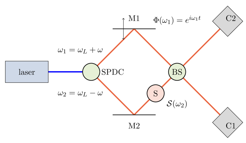
In this paper, we provide a precise connection between a material sample, described in terms of a model Hamiltonian, and the resulting signal in the context of the interference experiment described by Kalashnikov et al. in Ref.Kalashnikov2016b , using the Dicke model for an ensemble of two-level atoms as input.PhysRev.93.99 The Dicke model is an important test-case since it undergoes a dynamical phase transition. Such behaviour was recently observed by Klinder et al. by coupling an atomic Bose-Einstein condensate to an optical cavity.kilnder:2015 We begin with a brief overview of the photon coincidence experiment and the preparation of two-photon entangled states, termed “Bell-states”. We then use the input/output approach of Gardner and Collett Gardiner1985 to develop a means for computing the transmission function for a –material system placed in one of the arms of the Hong-Ou-Mandel (HOM) apparatus sketched in Fig. 1.
II Quantum interference of entangled photons
We consider the interferometric scheme implemented by Kalashnikovet al. Kalashnikov2016b A CW laser beam is incident on a nonlinear crystal, creating an entangled photon pair state by spontaneous parametric down-conversion (SPDC), which we shall denote as a Bell state
| (1) |
where is the bi-photon field amplitude and creates a photon with frequency in either the signal or idler branch. The ket is the vacuum state and denotes a two photon state.
In general, energy conservation requires that the entangled photons generated by spontaneous parametric down conversion (SPDC) obey . Similarly, conservation of photon momentum requires . By manipulating the SPDC crystal, one can generate entangled photon pairs with different frequencies. As a result, the bi-photon field is strongly anti-correlated in frequency with
| (2) |
where is the central frequency of the bi-photon field. This aspect was recently exploited in Ref. Kalashnikov2016a , which used a visible photon in the idler branch and an infrared (IR) photon in the signal branch, interacting with the sample.
As sketched in Figure 1, both signal and idler are reflected back towards a beam-splitter (BS) by mirrors M1 and M2. M1 introduces an optical delay with transmission function which we will take to be of modulo 1. In the other arm, we introduce a resonant medium at S with transmission function . Not shown in our sketch is an optional pumping laser for creating a steady state exciton density in S.
Upon interacting with both the delay element and the medium, the Bell-state can be rewritten as
Finally, the two beams are recombined by a beam splitter (BS) and the coincidence rate is given by
| (4) | |||||
We assume that the delay stage is dispersionless with and re-write equation 4 as
| (5) | |||||
where is the time lag between entangled photons traversing the upper and lower arms of the HOM apparatus. This is proportional to the counting rate of coincident photons observed at detectors C1 and C2 and serves as the central experimental observable.
III Results
A crucial component of our approach is the action of the sample at S which introduces a transmission function into the final Bell state. We wish to connect this function to the dynamics and molecular interactions within the sample. To accomplish this, we use the input/output formulation of quantum optics and apply this to an ensemble of identical 2-level states coupled to a common photon mode.PhysRevA.75.013804 Technical details of our approach are presented in the Methods section of this paper. In short, we begin with a description of the material system described by two-level spin states coupled to common set of photon cavity modes.
| (6) | |||||
where are local spin-1/2 operators for site , is the local excitation energy, and is the coupling between the th photon mode and the th site, which we will take to be uniform over all sites. We introduce as the decay rate of a cavity photon. We allow the photons in the cavity (S) to exchange quanta with photons in the HOM apparatus and derive the Heisenberg equations of motion corresponding to input and output photon fields within a steady state assumption. This allows us to compute the scattering matrix connecting an incoming photon with frequency from the field to an outgoing photon with frequency returned to the field viz.
| (7) |
where are Møller operators that propagate an incoming (or outgoing) state from to where it interacts with the sample. or from to an outgoing (or incoming) state at and give the -matrix in the form of a response function
| (8) |
where the are fluctuations in the output photon field about a steady-state solution. The derivation of for the Dicke model and its incorporation into equation 5 is a central result of this work and is presented in the Methods section of this paper. In general, is a complex function with a series of poles displaced above the real axis and we employ a sync-transformation method to integrate equation 5. The approach can be applied to any model Hamiltonian system and provides the necessary connection between a microscopic model and its predicted photon coincidence.
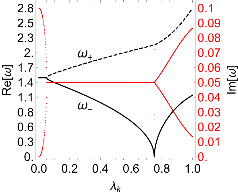
Before discussing the results of our calculations, it is important to recapitulate a number of aspects of the Dicke model and how these features are manifest in the photon coincidence counting rates. As stated already, we assume that the sample is in a steady state by exchanging the photons in the HOM apparatus with photons within the sample cavity and that can be described within a linear-response theory. Because the cavity photons become entangled with the material excitations, the excitation frequencies are split into upper photonic () and lower excitonic () branches. These frequencies are complex corresponding to the exchange rate between cavity and HOM photons.
At very low values of , the real frequencies are equal and . In this over-damped regime, photons leak from the cavity before the photon/exciton state has undergone a single Rabi oscillation. At the system becomes critically damped and for and the degeneracy between the upper and lower polariton branches is lifted. As increases above a critical value given by
| (9) |
the system undergoes a quantum phase transition when . Above this regime, excitations from the non-equilibrium steady-state become collective and super-radiant. For our numerical results, unless otherwise noted we use dimensionless quantities, taking for both the exciton frequency and cavity mode frequency, for the cavity decay. These give a critical value of .
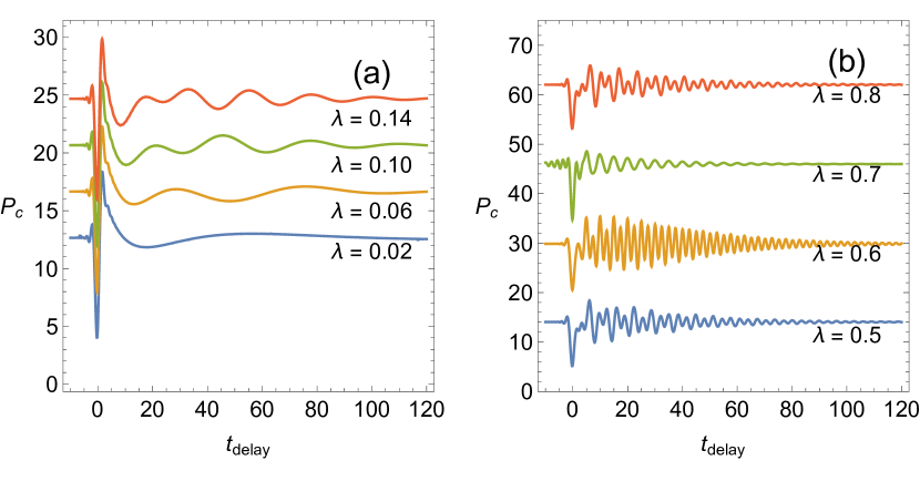
We first consider the photon coincidence in the normal regime. Figures 2(a,b) show the variation of the photon coincidence count when the laser frequency is resonant with the excitons (). For low values of , the system is in the over-damped regime and the resulting coincidence scan reveals a slow decay for positive values of the time-delay. This is the perturbative regime in which the scattering photon is dephased by the interaction with the sample, but there is insufficient time for the photon to become entangled with the sample. For , the scattering photon is increasingly entangled with the material and further oscillatory structure begins to emerge in the coincidence scan.
In the strong coupling regime, becomes increasingly oscillatory with contributions from multiple frequency components. The origin of the structure is further revealed upon taking the Fourier cosine transform of (equation 5) taking the bandwidth of the bi-photon amplitude to be broad enough to span the full spectral range. The first two terms in the integral of equation 5 are independent of time and simply give a background count and can be ignored for purpose of analysis. The third term depends upon the time delay and is Fourier-cosine transform of the bi-photon amplitude times the scattering amplitudes,
| (10) |
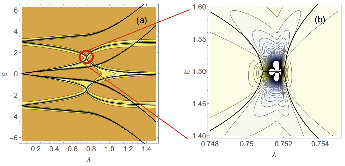
As we show in the Methods, has a series of poles on the complex plane that correspond to the frequency spectrum of fluctuations about the matter-radiation steady-state as given by the eigenvalues of in equation 58 in the Methods. In Figure 3(a,b) we show the evolution of pole-structure of superimposed over the Fourier-cosine transform of the coincidence counts () with increasing coupling revealing that that both excitonic and photonic branches contribute to the overall photon coincidence counting rates.
A close examination of the pole structure in the vicinity of the phase transition reveals that two of the modes become degenerate over a small range of but with different imaginary components indicating that the two modes decay at different rates. This is manifest in Figure 3b by the rapid variation and divergence in the about . Kopylov2013 While the parametric width of this regime is small, it depends entirely upon the rate of photon exchange between the cavity and the laser field ().
IV Discussion
We present here a formalism and method for connecting the photon coincidence signals for a sample placed in a HOM apparatus to the optical response of the coupled photon/material system. Our formalism reveals that by taking the Fourier transform of the coincidence signal reveals the underlying pole structure of the entangled material/photon system. Our idea hinges upon an assumption that the interaction with the material preserves the initial entanglement between the two photons and that sample on the entanglement introduces an additional phase lag to one of the photons which we formally introduce in the form of a scattering response function . The pole-structure in the output comes about from the further quantum entanglement of the signal photon with the sample.
Encoded in the time-delay signals is important information concerning the inner-workings of a quantum phase transition. Hence, we conclude that entangled photons with interferometric detection techniques provide a viable and tractable means to extract precise information concerning light-matter interactions. In particular, the approach reveals that at the onset of the symmetry-breaking transition between normal and super-radiant phases, two of the eigenmodes of the light-matter state exhibit distinctly different lifetimes. This signature of an intrinsic aspect of light-matter entanglement may be observed in a relatively simple experimental geometry with what amounts to a linear light-scattering/interferometry set up.
At first glance, it would appear that using quantum photons would not offer a clear advantage over more standard spectroscopies based upon a semi-classical description of the radiation field. However, the entanglement variable adds an additional dimension to the experiment allowing one to preform what would ordinarily be a non-linear experiment using classical light as a linear experiment using quantized light. The recent works by Kalashnikov et al. that inspired this work are perhaps the proverbial tip of the iceberg. Kalashnikov2016a ; Kalashnikov2016b
Acknowledgments
The work at the University of Houston was funded in part by the National Science Foundation (CHE-1664971, MRI-1531814) and the Robert A. Welch Foundation (E-1337). AP acknowledges the support provided by Los Alamos National Laboratory Directed Research and Development (LDRD) Funds. CS acknowledges support from the School of Chemistry & Biochemistry and the College of Science of Georgia Tech. JJ acknowledges the support of the Army Research Office (W911NF-13-1-0162). ARSK acknowledges funding from EU Horizon 2020 via Marie Sklodowska Curie Fellowship (Global) (Project No. 705874).
Appendix A Preparation of Entangled States
We review here the preparation of the entangled states as propagated to the coincidence detectors in Fig. 1. The initial laser beam produces an entangled photon pair by spontaneous parametric down-conversion at B, with state which we shall denote as a Bell state
| (11) | |||||
| (12) |
where is the bi-photon field amplitude and creates a photon with frequency in either the idler (I) or signal (S) arm of the HOM apparatus. The ket is the vacuum state and denotes a two photon state. The two photons are reflected back towards a beam-splitter (BS) by mirrors M1 and M2. M1 introduces an optical delay with transmission function which we will take to be of modulo 1. In the other arm, we introduce a resonant medium at S with transmission function . Upon interacting with both the delay element and the medium, the Bell-state can be rewritten as
Finally, the two beams are re-joined by a beam-splitter (BS) producing the mapping
whereby creates a photon with frequency in the exit channel. This yields a final Bell state
| (14) | |||||
The coincidence count rate is determined only by the real part of photon creation term, so we write
| (15) | |||||
and
| (16) | |||||
Upon taking and , and changing the integration variable we obtain equation 5 in the text.
Appendix B Input/Output formalism
Our theoretical approach is to treat S as a material system interacting with a bath of quantum photons. We shall denote our “system” as those degrees of freedom describing the material and the photons directly interacting with the sample, described by and assume that the photons within sample cavity are exchanged with external photons in the bi-photon field,
| (17) |
where are boson operators for photons in the laser field, and are boson operators for cavity photons in the sample that directly interact with the material component of the system.
The Heisenberg equations of motion for the reservoir and system photon modes are given by
| (18) |
and
| (19) |
where the integration range is over all . We can integrate formally the equations for the reservoir given either the initial or final states of the reservoir field
| (22) |
We shall eventually take and and require that the forward-time propagated and reverse-time propagated solutions are the same at some intermediate time . If we assume that the coupling is constant over the frequency range of interest, we can write
where is the rate that energy is exchanged between the reservoir and the system. This is the (first) Markov approximation.
Using these identities, one can find the Heisenberg equations for the cavity modes as
| (23) |
where is the Hamiltonian for the isolated system. We can now cast the external field in this equation in terms of its initial condition:
| (24) | |||||
Let us define an input field in terms of the Fourier transform of the reservoir operators:
| (25) |
Since these depend upon the initial state of the reservoir, they are essentially a source of stochastic noise for the system. In our case, we shall use these as a formal means to connect the fields inside the sample to the fields in the laser cavity.
For the term involving , the integral over frequency gives a delta-function:
| (26) |
then
| (27) |
This gives the forward equation of motion.
| (28) |
We can also define an output field by integrating the reservoir backwards from time to time given a final state of the bath, .
| (29) |
This produces a similar equation of motion for the output field
| (30) |
Upon integration:
| (31) |
At the time , both equations must be the same, so we can subtract one from the other
| (32) |
to produce a relation between the incoming and outgoing components. This eliminates the non-linearity and explicit reference to the bath modes.
We now write as a vector of Heisenberg variables for the material system and cavity modes . Taking the equations of motion for the all fields to be linear and of the form
| (33) |
where is a matrix of coefficients which are independent of time. The input vector is non-zero for only the terms involving the input modes. We can also write a similar equation in terms of the output field; however, we have to account for the change in sign of the dissipation terms, so we denote the coefficient matrix as . In this linearized form, the forward and reverse equations of motion can be solved formally using the Laplace transform, giving
| (34) | |||||
| (35) |
These and the relation allows one to eliminate the external variables entirely:
| (36) |
This gives a precise connection between the input and output fields. More over, the final expression does not depend upon the assumed exchange rate between the internal and external photon fields. The procedure is very much akin to the use of Møller operators in scattering theory. To explore this connection, define as an operator which propagates an incoming solution at to the interaction at time and its reverse which propagates an out-going solution at back to the interaction at time .
| (37) |
and
| (38) | |||
| (39) |
Thus, we can write equation 36 as
| (40) |
To compute the response function, we consider fluctuations and excitations from a steady state solution:
| (41) |
The resulting linearized equations of motion read
| (42) |
implying a formal solution of
| (43) |
From this we deduce that the eigenvalues and eigenvectors of give the fluctuations in terms of the normal excitations about the stationary solution. Using the input/output formalism, we can write the outgoing state (in terms of the Heisenberg variables) in terms of their input values:
where as given above, is a vector containing the fluctuations about the stationary values for each of the Heisenberg variables. The and are the coefficient matrices from the linearisation process. The input field satisfies and all other terms are zero. Thus, the transmission function is given by
| (45) |
In other words, the is the response of the system to the input field of the incoming photon state producing an output field for the out-going photon state.
Appendix C Dicke model for ensemble of identical emitters
Let us consider an ensemble of identical two-level systems corresponding to local molecular sites coupled to a set of photon modes described by .
| (46) | |||||
where are local spin-1/2 operators for site , is the local excitation energy, and is the coupling between the th photon mode and the th site, which we will take to be uniform over all sites. Defining the total angular momentum operators
and
as the total angular momentum operator, this Hamiltonian can be cast in the form in equation 46 by mapping the total state space of spin 1/2 states onto a single angular momentum state vector .
| (47) | |||||
Note that the ground state of the system corresponds to in which each molecule is in its electronic ground state. Excitations from this state create up to excitons within the system corresponding to the state . Intermediate to this are multi-exciton states which correspond to various coherent superpositions of local exciton configurations. For each value of the wave vector one obtains the following Heisenberg equations of motion for the operators
| (48) | |||||
| (49) | |||||
| (50) | |||||
| (51) |
where is gives the decay of photon into the reservoir. These are non-linear equations and we shall seek stationary solutions and linearize about them.
| (52) |
with
| (58) |
where , , and denote the steady state solutions. Where we have removed from the equations of motion by simply rescaling the variables. The model has both trivial and non-trivial stationary solutions corresponding to the normal and super-radiant regimes. For the normal regime,
| (60) |
and
| (61) |
which correspond to the case where every spin is excited or in the ground state. Since we are primarily interested in excitations from the electronic ground state, we initially focus our attention to these solutions.
Non-trivial solutions to these equations predict that above a critical value of the coupling , the system will undergo a quantum phase transition to form a super-radiant state. It should be pointed out that in the original Dicke model, above the critical coupling, the system is no longer gauge invariant leading to a violation of the Thomas-Reiche-Kuhn (TRK) sum rule. Gauge invariance can be restored; however, the system no longer undergoes a quantum phase transition.Rzazewski:1975 However, for a driven, non-equilibrium system such as presented here, the TRK sum rule does not apply and the quantum phase transition is a physical effect.
The non-trivial solutions for the critical regime are given by
| (62) | |||||
| (63) | |||||
| (64) |
The (real) eigenvalues of gives 4 non-zero and 1 trivial normal mode frequencies (for ), which we shall denote as
one obtains the critical coupling constant
| (66) |
Figure 4 gives the normal mode spectrum for a resonant system with and (in reduced units).

Appendix D Evaluation of integrals in Eqs. 5 and 4
The integral in Eq 5 for the photon coincidence can be problematic to evaluate numerically given the oscillatory nature of the sinc function in . To accomplish this, we use define a sinc-transformation based upon using the identity
| (67) |
which yields
| (68) |
From this we can re-write each term in Eqs. 5 in the form
| (69) | |||||
| (70) |
whereby we denote
| (71) |
The integrand is highly oscillatory along the -axis; however, for non-zero , becomes a Gaussian integral under coordinate transformation obtained by completing the square:
| (72) | |||||
| (73) | |||||
| (74) |
For , we take , and for , we take . Solving for yields: and , respectively. In short, the optimal contour of the Gaussian integral is obtained by rotating by from the real-axis in the counter-clockwise direction for the case of and by in the clockwise direction for the case of as indicated in Fig. 5.
The spectral response has a number of poles on the complex plane above the real- axis. We now use the residue theorem to evaluate the necessary poles which result as the contour rotates from the real axis to the complex axis. The 8 second order poles, , are defined by roots of the denominators and and located above the real axis at locations symmetrically placed around the origin. For the counter-clockwise rotation (), poles included to the right of the real crossing point will be added and those to the left will be ignored () ; whereas for a clockwise rotation (), the left-hand poles will be subtracted and the right-hand poles will be ignored (). For the unique case , all poles are summed ().
| (75) |
Thus, we obtain
| (76) | |||||
| (77) | |||||
| (78) | |||||
| (79) | |||||
whereby , , and are summed over the left, right, or all poles, respectively. The resulting expressions are analytic (albeit lengthy) and defined by exponentials and low order polynomials. Completion of the and integrals yield an exact expression for the response.
References
- [1] Eric Brannen and H. I. S. Ferguson. The Question of Correlation between Photons in Coherent Light Rays. Nature, 178(4531):481–482, sep 1956.
- [2] R. Hanbury Brown and R. Q. Twiss. A Test of a New Type of Stellar Interferometer on Sirius. Nature, 178(4541):1046–1048, nov 1956.
- [3] E. M. Purcell. The Question of Correlation between Photons in Coherent Light Rays. Nature, 178(4548):1449–1450, dec 1956.
- [4] R. H. Brown and R. Q. Twiss. Interferometry of the Intensity Fluctuations in Light. I. Basic Theory: The Correlation between Photons in Coherent Beams of Radiation. Proceedings of the Royal Society A: Mathematical, Physical and Engineering Sciences, 242(1230):300–324, nov 1957.
- [5] R. H. Brown and R. Q. Twiss. Interferometry of the Intensity Fluctuations in Light II. An Experimental Test of the Theory for Partially Coherent Light. Proceedings of the Royal Society A: Mathematical, Physical and Engineering Sciences, 243(1234):291–319, jan 1958.
- [6] U. Fano. Quantum Theory of Interference Effects in the Mixing of Light from Phase-Independent Sources. American Journal of Physics, 29(8):539–545, aug 1961.
- [7] H. Paul. Photon antibunching. Reviews of Modern Physics, 54(4):1061–1102, oct 1982.
- [8] Nicolas Gisin, Grégoire Ribordy, Wolfgang Tittel, and Hugo Zbinden. Quantum cryptography. Rev. Mod. Phys., 74:145–195, Mar 2002.
- [9] Nicolas Gisin and Rob Thew. Quantum communication. Nat Photon, 1(3):165–171, 03 2007.
- [10] E Knill, R Laflamme, and G J Milburn. A scheme for efficient quantum computation with linear optics. Nature, 409(6816):46–52, jan 2001.
- [11] Oleksiy Roslyak, Christoph A. Marx, and Shaul Mukamel. Nonlinear spectroscopy with entangled photons: Manipulating quantum pathways of matter. Phys. Rev. A, 79:033832, Mar 2009.
- [12] Gabriela Barreto Lemos, Victoria Borish, Garrett D Cole, Sven Ramelow, Radek Lapkiewicz, and Anton Zeilinger. Quantum imaging with undetected photons. Nature, 512(7515):409–12, aug 2014.
- [13] J. C. López Carreño and F. P. Laussy. Excitation with quantum light. I. Exciting a harmonic oscillator. Physical Review A, 94(6):063825, dec 2016.
- [14] J. C. López Carreño, C. Sánchez Muñoz, E. del Valle, and F. P. Laussy. Excitation with quantum light. II. Exciting a two-level system. Physical Review A, 94(6):063826, dec 2016.
- [15] Dmitry A Kalashnikov, Anna V Paterova, Sergei P Kulik, and Leonid A Krivitsky. Infrared spectroscopy with visible light. Nature Photonics, 10(2):98–101, jan 2016.
- [16] Dmitry A. Kalashnikov, Elizaveta V. Melik-Gaykazyan, Alexey A. Kalachev, Ye Feng Yu, Arseniy I. Kuznetsov, and Leonid A. Krivitsky. Time-resolved spectroscopy with entangled photons. arXiv://1611.02415 2016.
- [17] Frank Schlawin, Konstantin E. Dorfman, Benjamin P. Fingerhut, Shaul Mukamel, and S. Mukamel. Suppression of population transport and control of exciton distributions by entangled photons. Nature Communications, 4:1782, apr 2013.
- [18] Oleg Varnavski, Brian Pinsky, and Theodore Goodson. Entangled photon excited fluorescence in organic materials: An ultrafast coincidence detector. The Journal of Physical Chemistry Letters, 8(2):388–393, 2017. PMID: 28029793.
- [19] W. H. Zurek. Cosmological experiments in superfluid helium? Nature, 317(6037):505–508, 10 1985.
- [20] Paul D Nation and Miles P Blencowe. The trilinear Hamiltonian: a zero-dimensional model of Hawking radiation from a quantized source. New Journal of Physics, 12(9):095013, 2010.
- [21] R. H. Dicke. Coherence in spontaneous radiation processes. Phys. Rev., 93:99–110, Jan 1954.
- [22] Jens Klinder, Hans Keßler, Matthias Wolke, Ludwig Mathey, and Andreas Hemmerich. Dynamical phase transition in the open dicke model. Proceedings of the National Academy of Science, 112:3290–3295.
- [23] C. W. Gardiner and M. J. Collett. Input and output in damped quantum systems: Quantum stochastic differential equations and the master equation. Physical Review A, 31(6):3761–3774, jun 1985.
- [24] F. Dimer, B. Estienne, A. S. Parkins, and H. J. Carmichael. Proposed realization of the dicke-model quantum phase transition in an optical cavity qed system. Phys. Rev. A, 75:013804, Jan 2007.
- [25] Wassilij Kopylov, Clive Emary, and Tobias Brandes. Counting statistics of the dicke superradiance phase transition. Physical Review A, 87(4):043840, 2013.
- [26] K Rzażewski, K Wódkiewicz, and W Żakowicz. Phase transitions, two-level atoms, and the term. Physical Review Letters, 35(7):432, 1975.