Fine-Grained vs. Average Reliability for V2V Communications around Intersections

Abstract

Intersections are critical areas of the transportation infrastructure associated with 47% of all road accidents. Vehicle-to-vehicle (V2V) communication has the potential of preventing up to 35% of such serious road collisions. In fact, under the 5G/LTE Rel.15+ standardization, V2V is a critical use-case not only for the purpose of enhancing road safety, but also for enabling traffic efficiency in modern smart cities. Under this anticipated 5G definition, high reliability of 0.99999 is expected for semi-autonomous vehicles (i.e., driver-in-the-loop). As a consequence, there is a need to assess the reliability, especially for accident-prone areas, such as intersections. We unpack traditional average V2V reliability in order to quantify its related fine-grained V2V reliability. Contrary to existing work on infinitely large roads, when we consider finite road segments of significance to practical real-world deployment, fine-grained reliability exhibits bimodal behavior. Performance for a certain vehicular traffic scenario is either very reliable or extremely unreliable, but nowhere in relative proximity to the average performance.

I Introduction

Today’s machine-driven vehicles are primarily based on LiDARs, sensors, radars, cameras, GPS, and 3D digital mapping. Nonetheless, these vehicles are constrained by line-of-sight, and their practicality is significantly influenced by weather conditions, such as fog, sunbeams, heavy rain and snow. Meanwhile, vehicle-to-vehicle (V2V) communication is the only technology that enables autonomous vehicles to see around corners in highly urbanized settings in order to detect the presence of nearby vehicles and take preemptive action to avoid collisions. In fact, studies suggest that V2V communications may prevent up to 35% of serious accidents [1]. Moreover, in harsh weather conditions, V2V communication offers a more reliable alternative to sensors capability.

Evidently, for the purpose of enhancing road safety and traffic efficiency, there are numerous V2V use-cases that require careful investigation and analysis. According to the U.S. Department of Transportation, data assessed between 2010-2015 suggest that nearly half of all vehicular accidents occur at intersections [2]. What is more surprising is that the rate of intersection accidents remained steady over the years, and this is despite a growth in the number of vehicles on the roads and the continuous evolution of accident avoidance technology. As a result, carefully investigating the reliability of V2V communications around intersections and, in particular, blind urban junctions, where the signal strength diminishes significantly over very short distances, will enable us to explicitly measure the feasibility of seeing vehicles hindered by high-rise infrastructures near corners.

For scalability and interoperability, standardization of connected vehicles is exceptionally critical. Currently, two standards are in direct competition: (i) IEEE 802.11p, also known as direct short range communication (DSRC) [3]; and (ii) cellular-V2X (C-V2X) communications supported by 4G/LTE Rel.14+ [4, 5]. The ad hoc DSRC standard is defined and ready for utilization, whereas the ad hoc/network-based C-V2X is still under development for 5G/LTE Rel.15+ operation aimed near 2020. Meanwhile, highly autonomous vehicles will rely on machine learning capability, where extensive driving experience will be shared wirelessly to the cloud and to other units using V2X capability at multi-Gbps data rates. Other vehicles connected to the network will immediately upgrade their transportation system regarding a particular geographical region of interest without the need of time-consuming knowledge acquisition. For such intricate network, the potential of 5G/C-V2X is promising and directly suitable to these stipulated requirements.

Irrespective of the adapted standard, we ultimately need to develop analytical expressions that will serve as a useful mechanism to accurately quantify the extent of reliability for a certain V2V communication link. This analysis will also aid in identifying the contribution of relevant parameters for the purpose of designing and reconfiguring the vehicular ad hoc network (VANET). Road traffic modeling based on point processes is well suited to study such problems where techniques from stochastic geometry have been applied (e.g. [6, 7, 8, 9, 10, 11]). As for intersections, they were explicitly considered in [10], though only for suburban/rural scenarios over infinitely long roads. However, for the analytical expressions to have practical real-world relevance, they must build on plausible VANET scenarios coupled with channel models validated by precise measurement campaigns [12, 13].

The above-mentioned works in stochastic geometry allow the evaluation of the average reliability, obtained by averaging over different fading realizations and node placements. This average reliability may obscure the performance for specific node configuration [14], referred to as the fine-grained reliability. In this paper, we perform a study of the fine-grained reliability, dedicated to urban intersections which have particular propagation characteristics [15, 16, 17, 18], complementing and generalizing the results in [10, 11].

II System Model

II-A Network Model

The VANET formed around the intersection is described as follows. The position of the transmitter (TX) can be anywhere on the horizontal or vertical road. Without loss of generality, the receiver (RX) is confined to the horizontal road. Thus, $\mathbf{x}_{\text{$\mathrm{tx}$}}\!=\!x_{\mathrm{tx}}\mathbf{e}_{\mathrm{x}}+y_{\mathrm{tx}}\mathbf{e}_{\mathrm{y}}$ and $\mathbf{x}_{\mathrm{rx}}\!=\!x_{\mathrm{rx}}\mathbf{e}_{\mathrm{x}}$, where $x_{\mathrm{tx}},x_{\mathrm{rx}},y_{\mathrm{tx}}\in\mathbb{R}$, such that $x_{\mathrm{tx}}y_{\mathrm{tx}}\!=\!0$, where $\mathbf{e}_{\mathrm{x}}\!=\![1\,0]^{\mathrm{T}}$, $\mathbf{e}_{\mathrm{y}}\!=\![0\,1]^{\mathrm{T}}$. Other traffic vehicles are randomly positioned on both horizontal and vertical roads and follow a homogeneous Poisson point process (H-PPP) over bounded sets $\mathcal{B}_{\mathrm{x}}=\left\{x\in\mathbb{R},\,R_{\mathrm{x}}\in\mathbb{R}^{+}\bigl{|}\left|x\right|\leq R_{\mathrm{x}}\right\}$ and $\mathcal{B}_{\mathrm{y}}=\left\{y\in\mathbb{R},\,R_{\mathrm{y}}\in\mathbb{R}^{+}\bigl{|}\left|y\right|\leq R_{\mathrm{y}}\right\}$, such that $R_{\mathrm{x}}$ and $R_{\mathrm{y}}$ are road segments of the intersection region, and the vehicular traffic intensities are respectively given by $\lambda_{\mathrm{x}}$ and $\lambda_{\mathrm{y}}$. The interfering vehicles follow an Aloha MAC protocol and can transmit independently with a probability $p_{\mathrm{I}}\!\in\!\left[0,1\right]$. The following shorthand notations are accordingly used to refer to the geometry of interfering vehicles on each road, modeled by thinned H-PPPs

$$\Phi_{\mathrm{x}} =\left\{\mathbf{x}_{i}\right\}_{i=1,2,\ldots,n}\ \in\mathbb{R}^{n}\>\sim\thinspace\textrm{PPP}\left(p_{\mathrm{I}}\lambda_{\mathrm{x}},\mathcal{B}_{\mathrm{x}}\right)$$ (1)

$$\Phi_{\mathrm{y}} =\left\{\mathbf{x}_{j}\right\}_{j=1,2,\ldots,m}\in\mathbb{R}^{m}\sim\thinspace\textrm{PPP}\left(p_{\mathrm{I}}\lambda_{\mathrm{y}},\mathcal{B}_{\mathrm{y}}\right),$$ (2)

such that $n$ and $m$ are random Poisson distributed integers with mean $p_{\mathrm{I}}\lambda\left|\mathcal{B}\right|$, where $\left|\mathcal{B}\right|$ is the Lebesgue measure of bounded set $\mathcal{B}$. All vehicles, including TX, broadcast with the same power level $P_{\circ}$. The signal-to-interference-plus-noise-ratio ($\mathsf{SINR}$) threshold for reliable detection at the RX is set to $\beta$, in the presence of additive white Gaussian noise (AWGN) with power $N_{\circ}$. The $\mathsf{SINR}$ depends on the propagation channel, which we describe in the next subsection.

II-B Channel Models

The detected power at the RX from an active TX located at $\mathbf{x}$ is modeled by $P_{\mathrm{rx}}\left(\mathbf{x},\mathbf{x}_{\mathrm{rx}}\right)=P_{\circ}\ell_{\mathrm{ch}}\left(\mathbf{x},\mathbf{x}_{\mathrm{rx}}\right)$, which depends on transmit power $P_{\circ}$ and channel losses $\ell_{\mathrm{ch}}\left(\mathbf{x},\mathbf{x}_{\mathrm{rx}}\right)$. The components of channel losses are: average path loss $\ell_{\mathrm{pl}}\left(\mathbf{x},\mathbf{x}_{\mathrm{rx}}\right)$ that captures signal attenuation, shadow fading $\ell_{\mathrm{s}}\left(\mathbf{x},\mathbf{x}_{\mathrm{rx}}\right)$ that captures the impact of random obstacles, and small-scale fading $\ell_{\mathrm{f}}\left(\mathbf{x}\right)$ that accounts for the non-coherent addition of signal components. For the purpose of tractability, we implicitly consider shadow fading to be inherent within the H-PPP, and thus regard $\ell_{\mathrm{ch}}\left(\mathbf{x},\mathbf{x}_{\mathrm{rx}}\right)\simeq\ell_{\mathrm{pl}}\left(\mathbf{x},\mathbf{x}_{\mathrm{rx}}\right)\ell_{\mathrm{f}}\left(\mathbf{x}\right)$ [19]. We model $\ell_{\mathrm{f}}\left(\mathbf{x}\right)\sim\textrm{Exp}\left(1\right)$ as Rayleigh fading, independent with respect to $\mathbf{x}$. The path loss $\ell_{\mathrm{pl}}\left(\mathbf{x},\mathbf{x}_{\mathrm{rx}}\right)$ for different channel environments is described below.

II-B1 Suburban/Rural Channel

The average path loss model for V2V propagation adheres to an inverse power-law [13, 12]; thus

$$\ell_{\mathrm{pl}}^{\mathrm{s}}\left(\mathbf{x},\mathbf{x}_{\mathrm{rx}}\right)=A_{\circ}\left\|\mathbf{x_{\mathrm{rx}}}-\mathbf{x}\right\|^{-\alpha} \ \ \ \ \mathbf{x}\neq\mathbf{x_{\mathrm{rx}}}\mathrm{.}$$ (3)

In this expression, $\left\|\cdot\right\|$ is the $l_{2}$-norm, $A_{\circ}$ corresponds to the LOS/WLOS path loss coefficient, which is primarily a function of operating frequency $f_{\circ}$, path loss exponent $\alpha\!>\!1$, reference distance $d_{\circ}$, and antenna heights $h\left(\mathbf{x}\right)$ and $h\left(\mathbf{x}_{\mathrm{rx}}\right)$.

II-B2 Urban Channel

For metropolitan intersections where the concentration of high-rise and impenetrable metallic-based buildings and structures are prevalent, the previous Euclidean model is rather unrealistic. Real-world measurements of V2V communications operating at 5.9 GHz were conducted at different urban intersection locations, leading to the VirtualSource11p path loss model [17, 18], adapted here as

$$\ell_{\mathrm{pl}}^{\mathrm{u}}\left(\mathbf{x},\mathbf{x}_{\mathrm{rx}}\right)=$$

$$\ \ \ \ \ \ \ \begin{cases}A_{\circ}^{\prime}\left(\left\|\mathbf{x}\right\|\cdot\left\|\mathbf{x}_{\mathrm{rx}}\right\|\right)^{-\alpha}&\min\left(\left\|\mathbf{x}\right\|=\left|y\right|,\left\|\mathbf{x}_{\mathrm{rx}}\right\|\right)>\triangle\\ A_{\circ}\left(\left\|\mathbf{x}\right\|+\left\|\mathbf{x}_{\mathrm{rx}}\right\|\right)^{-\alpha}&\min\left(\left\|\mathbf{x}\right\|=\left|y\right|,\left\|\mathbf{x}_{\mathrm{rx}}\right\|\right)\leq\triangle\\ A_{\circ}\left\|\mathbf{x}_{\mathrm{rx}}-\mathbf{x}\right\|^{-\alpha}&\left\|\mathbf{x}\right\|=\left|x\right|;\ \mathbf{x}\neq\mathbf{x}_{\mathrm{rx}},\end{cases}$$ (4)

where $\triangle\leq\min\left(R_{\mathrm{x}},R_{\mathrm{y}}\right)$ is the break-point distance (typically on the order of the road width), and $A_{\circ},A^{\prime}_{\circ}$ are suitable path loss coefficients [20]. The first case in (4) refers to NLOS link, the second to WLOS, and the third to LOS.

III Transmission Reliability

III-A Average Reliability

The goal is to determine the success probability $\mathcal{P}_{\mathrm{c}}\left(\beta,\mathbf{x}_{\text{$\mathrm{tx}$}},\mathbf{x}_{\mathrm{rx}}\right)\triangleq\Pr\left(\mathsf{SINR}\geq\beta\right)$, where $\Pr\left(\cdot\right)$ is averaged over small-scale fading of the channel $\ell_{\mathrm{f}}$ and point processes $\Phi_{\mathrm{x}}$ and $\Phi_{\mathrm{y}}$; and where

$$\mathsf{SINR} =\frac{\ell_{\mathrm{f}}\left(\mathbf{x}_{\text{$\mathrm{tx}$}}\right)\ell_{\mathrm{pl}}\left(\mathbf{x}_{\text{$\mathrm{tx}$}},\mathbf{x}_{\mathrm{rx}}\right)}{{\displaystyle\sum_{\mathbf{x}\in\Phi_{\mathrm{x}}\cup\Phi_{\mathrm{y}}}\ell_{\mathrm{f}}\left(\mathbf{x}\right)\ell_{\mathrm{pl}}\left(\mathbf{x},\mathbf{x}_{\mathrm{rx}}\right)+\gamma_{\circ}}},$$ (5)

in which $\gamma_{\circ}\!\!=\!\!N_{\circ}/P_{\circ}$. We introduce a normalized aggregate interference associated with a process $\Phi$ as: $I\left(\Phi\right)\triangleq\sum_{\mathbf{x}\in\Phi}\ell_{\mathrm{f}}\left(\mathbf{x}\right)\ell_{\mathrm{pl}}\left(\mathbf{x},\mathbf{x}_{\mathrm{rx}}\right)$. Solving for the exponentially distributed fading of the wanted link, and taking the expectation of the probability with respect to interference, we get

$$\mathcal{P}_{\mathrm{c}}\left(\beta,\mathbf{x}_{\text{$\mathrm{tx}$}},\mathbf{x}_{\mathrm{rx}}\right) =\exp\bigl{(}-\beta^{\prime}\gamma_{\circ}\bigr{)}\thinspace\times\thinspace\mathbb{E}_{I_{\mathrm{x}}}\left\{\exp\bigl{(}-\beta^{\prime}I\left(\Phi_{\mathrm{x}}\right)\bigr{)}\right\}\ \ \$$

$$\times\thinspace\mathbb{E}_{I_{\mathrm{y}}}\left\{\exp\bigl{(}-\beta^{\prime}I\left(\Phi_{\mathrm{y}}\right)\bigr{)}\right\},$$ (6)

where $\beta^{\prime}=\beta/\ell_{\mathrm{pl}}\left(\mathbf{x}_{\text{$\mathrm{tx}$}},\mathbf{x}_{\mathrm{rx}}\right)$, the success probability in the absence of interference is simply $\exp\bigl{(}-\beta^{\prime}\gamma_{\circ}\bigr{)}$, and the remaining factors capture the degradation of the average reliability due to independent aggregate interference from the horizontal and vertical roads [11].

III-B Fine-Grained Reliability

The success probability $\mathcal{P}_{\mathrm{c}}\left(\beta,\mathbf{x}_{\text{$\mathrm{tx}$}},\mathbf{x}_{\mathrm{rx}}\right)$ provides a high-level performance assessment averaged over all possible vehicular traffic realizations and channel. Unpacking this average reliability metric and looking at it at the fine-grained or meta-level demands that we study the success probability of the individual links. In other words, we need to explore the meta distribution of the $\mathsf{SINR}$ [14]; defined, using the Palm probability of the point process $\mathbb{P}^{o}\left(\cdot\right)$, as

$$F_{\mathrm{r}}\left(\beta,p\right) \thinspace\triangleq\thinspace\mathbb{P}^{o}\Bigl{(}\thinspace\Pr\left(\mathsf{SINR}\geq\beta\thinspace|\thinspace\Phi_{\mathrm{x}}\cup\Phi_{\mathrm{y}}\right)\geq p\thinspace\Bigr{)}\mathrm{.}$$ (7)

Introducing $p_{\mathrm{c}}\left(\beta\right)\triangleq\Pr\left(\mathsf{SINR}\geq\beta\thinspace|\thinspace\Phi_{\mathrm{x}}\cup\Phi_{\mathrm{y}}\right)$ and $p_{\mathrm{out}}\left(\beta\right)=1-p_{\mathrm{c}}\left(\beta\right)$ respectively as the conditional success probability and conditional outage probability, given the point process $\Phi_{\mathrm{x}}\cup\Phi_{\mathrm{y}}$, and where $p\!\in\!\left[0,1\right]$ is a conditional success reliability constraint. Thus, the meta distribution $F_{\mathrm{r}}\left(\beta,p\right)$ is basically the fraction of vehicular traffic realizations that achieve reliability, in which reliability is prescribed by the target value assigned to $p$, and $\beta$ refers to the $\mathsf{SINR}$ threshold.

Using the Palm expectation $\mathbb{E}^{o}\left(\cdot\right)$, we can obtain the average reliability of success from the meta distribution. In other words, the first moment of $p_{\mathrm{c}}\left(\beta\right)$ is the average reliability of success, i.e., $\mathbb{E}^{o}\left(p_{\mathrm{c}}\left(\beta\right)\right)=\mathcal{P}_{\mathrm{c}}\left(\beta,\mathbf{x}_{\text{$\mathrm{tx}$}},\mathbf{x}_{\mathrm{rx}}\right)$. Meanwhile, rather than obtaining the exact meta distribution through the Gil-Pelaez theorem [21], recent meta distribution related works suggest that the moments could be used to approximate $F_{\mathrm{r}}\left(\beta,p\right)$. In fact, the Beta probability density function (which only requires the first and second moments) is reported to yield high accuracy [14, 22, 23]:

$$F_{\mathrm{r}}\left(\beta,p\right)\thinspace\approx\thinspace\frac{p^{a-1}(1-p)^{b-1}}{B(a,b)},$$ (8)

where $B(a,b)$ is the Beta function, which serves as a normalization constant. The parameters of the Beta distribution can be estimated from $N$ realizations of $x\coloneqq\Pr\left(\mathsf{SINR}\geq\beta\thinspace|\thinspace\Phi_{\mathrm{x}}\cup\Phi_{\mathrm{y}}\right)$, say $x_{1},\ldots,x_{N}\in[0,1]$ using a methods of moments estimator. Introducing the estimates of the mean $\bar{x}=\sum_{n}x_{n}/N$, variance $v=\sum_{n}(x_{n}-\bar{x})^{2}/(N-1)$, and odds $o=(1-\bar{x})/\bar{x}$ , we find that $\hat{a}(\mathbf{x})=\bar{x}\left(o/v-1\right)$ and $\hat{b}(\mathbf{x})=o\,\hat{a}(\mathbf{x})$, provided the estimates are non-negative.

TABLE I: Simulation Parameters

system parameters
target success probability	$\mathcal{P}_{\mathrm{target}}=0.9$
transmit power	$P_{\circ}=20$ dBmW
AWGN floor	$N_{\circ}=-99$ dBmW
RX sensitivity	$\beta=8$ dB (if $B=40$ MHz; $r_{\mathrm{th}}\simeq 115$ Mbps)
channel propagation
operating frequency	$f_{\circ}=5.9$ GHz
reference distance	$d_{\circ}=10$ m
break-point distance	$\triangle=15$ m
path loss exponent	$\alpha=2$ (suburban); $1.68$ (urban)
LOS/WLOS path loss coefficient	$A_{\circ}\!=\!-37.86+10\alpha$  dBm
NLOS path loss coefficient	$A_{\circ}^{\prime}\!=\!-38.32+\left(7\!+\!10\log_{10}\triangle\right)\!\alpha$  dBm
vehicular traffic and geometry
traffic intensity	$\lambda=0.01$ # / m
size of road segment	$R=200$ m (practical); $10$ km (stress-test)
RX distance from junction point	$\left\|\mathbf{x}_{\mathrm{rx}}\right\|=50$ m
max. separation for reliable V2V com.	$d_{\mathrm{target}}=100$ m
max. TX/RX Manhattan separation	$d_{\mathrm{max}}=140$ m

IV Simulations and Discussion

IV-A Simulation Setup

Using the parameters shown in Table I, we evaluate the success probability under various conditions and scenarios. In particular, we set the vehicular traffic on both roads to be the same, i.e., $\lambda_{\mathrm{x}}\!=\!\lambda_{\mathrm{y}}\!=\!\lambda\!=\!0.01$ #/m. For identical road segments $R_{\mathrm{x}}\!=\!R_{\mathrm{y}}\!=\!R$, we consider $R\!\in\!\{200\,\mathrm{m},10\,\mathrm{km}\}$. Next, we assume a fixed RX on the horizontal road, with $\mathbf{x}_{\mathrm{rx}}\!=\![-50,0]^{\mathrm{T}}$ m; and a TX that could take different positions, up to a Manhattan separation of $d_{\mathrm{max}}\!=\!140$ m away from the RX, i.e., starting at $\mathbf{x}_{\mathrm{tx}}\!=\![-50,0]^{\mathrm{T}}$ m via $\mathbf{x}_{\mathrm{tx}}\!=\![0,0]^{\mathrm{T}}$ m up to $\mathbf{x}_{\mathrm{tx}}\!=\![0,+90]^{\mathrm{T}}$ m. To ensure a tolerable worst-case level of average performance, the success probability must achieve a certain preassigned target value, here set to

$$\mathcal{P}_{\mathrm{c}}\left(\beta,\mathbf{x}_{\text{$\mathrm{tx}$}},\mathbf{x}_{\mathrm{rx}}\right)\thinspace\geq\thinspace\mathcal{P}_{\mathrm{target}}=0.9,$$ (9)

over the intersection deployment region specified by $\mathcal{B}_{\mathrm{x}}\cup\mathcal{B}_{\mathrm{y}}$, and for all V2V communication pairs under consideration with positions $\mathbf{x}_{\mathrm{tx}}$ and $\mathbf{x}_{\mathrm{rx}}$. As design parameters, we consider the transmit probability $p_{\mathrm{I}}$ and its relation to road segments $R_{\mathrm{x}}$ and $R_{\mathrm{y}}$. Solving for the transmit probability in this design criteria, we find that $p_{\mathrm{I}}\leq p_{\mathrm{I}}^{\ast}\left(R\right)$, where the optimum probability was derived in [20]. In other words, with $p_{\mathrm{I}}\leq p_{\mathrm{I}}^{\ast}\left(R\right)$, $\mathcal{P}_{\mathrm{c}}\left(\beta,\mathbf{x}_{\text{$\mathrm{tx}$}},\mathbf{x}_{\mathrm{rx}}\right)\geq 0.9$, provided the RX remains fixed, the TX can have different positions, while $\left\|\mathbf{x}_{\mathrm{rx}}-\mathbf{x}_{\mathrm{tx}}\right\|_{1}\leq\left\|\mathbf{x}_{\mathrm{rx}}-\tilde{\mathbf{x}}_{\mathrm{tx}}\right\|_{1}$, where $\left\|\cdot\right\|_{1}$ is the $l_{1}$-norm and $\tilde{\mathbf{x}}_{\mathrm{tx}}$ is the TX position at target (i.e., at the worst-case position where target reliability is still fulfilled).

IV-B Sensitivity of Fine-Grained Reliability to TX/RX Separation

We aim to gain insight into the meta distribution for the $\mathbf{x}_{\text{$\mathrm{tx}$}}$ and $\mathbf{x}_{\mathrm{rx}}$ position variables, obtained from outage probability conditioned on a traffic realization, and as a function of TX/RX Manhattan separation. For every TX/RX position pair, we consider 10000 PPPs and for each PPP, 5000 fading realizations. The outage probability per intersection traffic of the point process, i.e., $\Pr\left(\mathsf{SINR}\leq\beta\thinspace|\thinspace\Phi_{\mathrm{x}}\cup\Phi_{\mathrm{y}}\right)$, can therefore be determined from extensive Monte Carlo simulations.

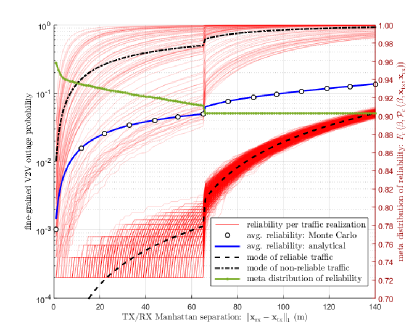
(a) practical deployment: $R=200$ m.

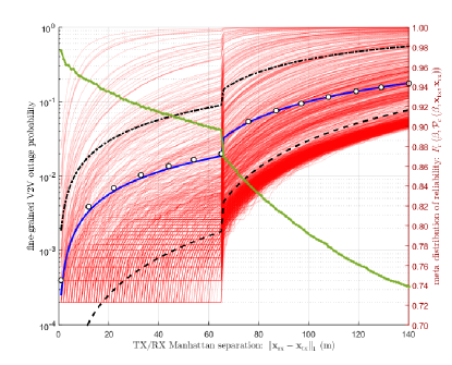
(b) stress-test: $R=10$ km.

Figure 1: Fine-grained reliability under network design as a function of TX/RX separation for urban intersection. The meta distribution of reliability is also shown over different V2V separations.

In Fig. 1a, considering the urban case and $R=200$ m (with $p_{\mathrm{I}}^{\ast}\left(R\right)=0.013$ to ensure an average success probability of 0.9 at $\left\|\mathbf{x}_{\mathrm{rx}}-\tilde{\mathbf{x}}_{\mathrm{tx}}\right\|_{1}=d_{\mathrm{target}}=100\,\mathrm{m}$), we plot the fine-grained outage probability (with an axis on the left), and the meta distribution (with an axis on the right) both as a function of $\left\|\mathbf{x}_{\mathrm{rx}}-\mathbf{x}_{\mathrm{tx}}\right\|_{1}$. We observe that the average outage probability $\mathcal{P}_{\mathrm{c}}\left(\beta,\mathbf{x}_{\text{$\mathrm{tx}$}},\mathbf{x}_{\mathrm{rx}}\right)$ (in blue) increases with $\left\|\mathbf{x}_{\mathrm{rx}}-\mathbf{x}_{\mathrm{tx}}\right\|_{1}$ and reaches the target value of 0.1 when $\left\|\mathbf{x}_{\mathrm{rx}}-\mathbf{x}_{\mathrm{tx}}\right\|_{1}=d_{\mathrm{target}}$. The corresponding meta distribution $F_{\mathrm{r}}\left(\beta,\mathcal{P}_{\mathrm{c}}\left(\beta,\mathbf{x}_{\text{$\mathrm{tx}$}},\mathbf{x}_{\mathrm{rx}}\right)\right)$ (in green) decreases, indicating that for low $\left\|\mathbf{x}_{\mathrm{rx}}-\mathbf{x}_{\mathrm{tx}}\right\|_{1}$, more PPPs achieve an outage below the average than at high separation values of $\left\|\mathbf{x}_{\mathrm{rx}}-\mathbf{x}_{\mathrm{tx}}\right\|_{1}$. Meanwhile, the sharp transitions of both curves at 65 m is due to the crossing of the vehicle from the WLOS region to the blind NLOS region. The figures also show the realizations of $\Pr\left(\mathsf{SINR}\leq\beta\thinspace|\thinspace\Phi_{\mathrm{x}}\cup\Phi_{\mathrm{y}}\right)$ for 1000 randomly chosen PPPs from the overall total of 10000, and the process is repeated with intervals of 1 m over different values of TX/RX Manhattan separation. From the plots, we see a clear bi-modal behavior, a PPP traffic realization either leads to communication reliability: far better than the requirement or far worse than the requirement, but not close to the average curve. By design, the average outage probability is mainly determined by the fraction of PPPs that meet the performance target, i.e., $F_{\mathrm{r}}\left(\beta,\mathcal{P}_{\mathrm{c}}\left(\beta,\mathbf{x}_{\text{$\mathrm{tx}$}},\mathbf{x}_{\mathrm{rx}}\right)\right)$, which for $\left\|\mathbf{x}_{\mathrm{rx}}-\mathbf{x}_{\mathrm{tx}}\right\|_{1}=100\,\mathrm{m}$ evaluates to $F_{\mathrm{r}}\left(\beta,0.9\right)\simeq 0.9$.

In Fig. 1b, we show the results for the stress-test scenario over a very large road segment corresponding to $R=10$ km (with $p_{\mathrm{I}}^{\ast}\left(R\right)=0.0021$ to ensure an average success probability of 0.9 at $\left\|\mathbf{x}_{\mathrm{rx}}-\tilde{\mathbf{x}}_{\mathrm{tx}}\right\|_{1}=d_{\mathrm{target}}=100\,\mathrm{m}$). We note a steeper decline in the meta distribution $F_{\mathrm{r}}\left(\beta,\mathcal{P}_{\mathrm{c}}\left(\beta,\mathbf{x}_{\text{$\mathrm{tx}$}},\mathbf{x}_{\mathrm{rx}}\right)\right)$, indicating a sharp deterioration of fine-grained reliability due to a larger interference region. This is also reflected in the outage probability curves per PPP realization, showing more spread than for the case of $R=200$ m.

Overall, we find that the generally accepted perception that performance for a particular traffic realization will be in relative proximity to the average reliability is misleading. This is especially true for interference limited over a short road segment of relevance to real-world V2V communications deployment.

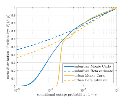
Figure 2: Meta distribution and Beta distribution approximation of reliability as a function of conditional outage probability for $R=10$ km over urban and suburban intersections.

IV-C Meta Distribution

We now fix $\left\|\mathbf{x}_{\mathrm{rx}}-\mathbf{x}_{\mathrm{tx}}\right\|_{1}=100\,\mathrm{m}$ and determine the complete meta distribution, $F_{\mathrm{r}}\left(\beta,p\right)$ from the simulation data. For all cases, the average outage probability is set to 0.1. We also determine the parameters of the Beta distribution through moment matching. For $R=10$ km (see Fig. 2), we observe that $F_{\mathrm{r}}\left(\beta,p\right)\simeq 0.8$ for $1-p=0.1$, which is congruent with the results from Fig. 1b. For $1-p\apprge 0.1$, the meta distribution and its Beta estimate are relatively well matched, predicting $F_{\mathrm{r}}\left(\beta,0.9\right)\in[0.75,0.8]$ for both urban and suburban cases. The match between the simulation and the Beta estimate break down when $1-p\apprle 0.03$. Here, the Beta distribution over-estimates the fraction of PPPs that lead to very low conditional outage. For $R=200$ m (see Fig. 3), the meta distribution shows a clear bimodal behavior, with a flat CDF for at least one order of magnitude of conditional outages. This effect is present for both urban and suburban intersections. The estimated Beta distribution cannot follow this trend, and thus severely overestimates $F_{\mathrm{r}}\left(\beta,p\right)$ for small conditional outage probabilities.

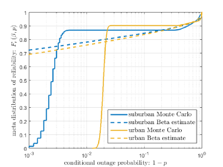
Figure 3: Meta distribution and Beta distribution approximation of reliability as a function of conditional outage probability for $R=200$ m over urban and suburban intersections.

Altogether, these results indicate that the average performance alone is not an adequate metric to assess communication reliability, but with different reasons for large and small road segments comprising an intersection. In addition, approximations using a Beta distribution can lead to overestimation in the low conditional outage regime.

V Conclusion

We evaluated the average and the fine-grained reliability for interference-limited V2V communications. The average communication reliability can be determined in closed-form notation using techniques from stochastic geometry. However, as the average is taken with respect to the channel environment and the interfering vehicular traffic, average reliability hides the underlying attributes of the random traffic. The meta distribution uncovers this, by describing the standalone reliability incurred from each PPP. We performed extensive Monte Carlo simulations to estimate both the average and the fine-grained communications reliability. Our results indicate that for small road segments, the meta distribution is bimodal so that PPPs are either not causing any interference or a lot of interference. Moreover, approximations of the meta distribution with a Beta distribution tend to be loose for short road segments.

References

- [1] “Study on the Deployment of C-ITS in Europe: Final Report,” EU, European Commission, Feb. 2016.
- [2] “Traffic Safety Facts 2015,” U.S. Dept. of Transportation, HS-812384, Jan. 2017.
- [3] “Part 11: Wireless LAN Medium Access Control (MAC) and Physical Layer (PHY) Specifications Amendment 6: Wireless Access in Vehicular Environments,” IEEE 802.11p standard, Jul. 2010.
- [4] “LTE, Rel.14.: Parallel feasibility study on LTE-based V2X Services,” RP-151109, Malm , Sweden, Jun. 15-18, 2015.
- [5] “LTE, Rel.14, Support for V2V services based on LTE sidelink,” RP-152293, Sitges, Spain, Dec. 7-10, 2015.
- [6] B. Błaszczyszyn, P. Mühlethaler, and Y. Toor, “Performance of MAC protocols in linear VANETs under different attenuation and fading conditions,” in Proc. IEEE Conference on Intelligent Transportation Systems, Oct. 2009, pp. 1–6.
- [7] B. Błaszczyszyn, P. Mühlethaler, and N. Achir, “Vehicular ad-hoc networks using slotted Aloha: point-to-point, emergency and broadcast communications,” in Proc. IFIP Wireless Days, Nov. 2012, pp. 1–6.
- [8] Y. Jeong, J. W. Chong, H. Shin, and M. Z. Win, “Intervehicle communication: Cox-Fox modeling,” IEEE Journal on Selected Areas in Communications, vol. 31, no. 9, pp. 418–433, Sep. 2013.
- [9] Z. Tong, H. Lu, M. Haenggi, and C. Poellabauer, “A stochastic geometry approach to the modeling of DSRC for vehicular safety communication,” IEEE Trans. on Intelligent Transportation Systems, vol. 17, no. 5, pp. 1448–1458, May 2016.
- [10] E. Steinmetz, M. Wildemeersch, T. Q. Quek, and H. Wymeersch, “A stochastic geometry model for vehicular communication near intersections,” in Proc. of IEEE Globecom Workshops, San Diego, CA, USA, Dec. 6-10, 2015, pp. 1–6.
- [11] M. Abdulla, E. Steinmetz, and H. Wymeersch, “Vehicle-to-vehicle communications with urban intersection path loss models,” in Proc. of IEEE Globecom, Washington DC, USA, Dec. 4-8, 2016, pp. 1–6.
- [12] C. F. Mecklenbrauker, A. F. Molisch, J. Karedal, F. Tufvesson, A. Paier, L. Bernado, T. Zemen, O. Klemp, and N. Czink, “Vehicular channel characterization and its implications for wireless system design and performance,” Proc. of the IEEE, vol. 99, no. 7, pp. 1189–1212, 2011.
- [13] J. Karedal, N. Czink, A. Paier, F. Tufvesson, and A. F. Molisch, “Path loss modeling for vehicle-to-vehicle communications,” IEEE Trans. on Vehicular Technology, vol. 60, no. 1, pp. 323–328, Jan. 2011.
- [14] M. Haenggi, “The meta distribution of the SIR in poisson bipolar and cellular networks,” IEEE Trans. on Wireless Communications, vol. 15, no. 5, pp. 2577–2589, Apr. 2016.
- [15] J. Karedal, F. Tufvesson, T. Abbas, O. Klemp, A. Paier, L. Bernado, and A. F. Molisch, “Radio channel measurements at street intersections for vehicle-to-vehicle safety applications,” in Proc. of the 71st IEEE Vehicular Technology Conference, May 2010, pp. 1–5.
- [16] M. Schack, J. Nuckelt, R. Geise, L. Thiele, and T. K rner, “Comparison of path loss measurements and predictions at urban crossroads for C2C communications,” in Proc. of the 5th European Conference on Antennas and Propagation (EuCAP), Apr. 2011, pp. 2896–2900.
- [17] T. Mangel, O. Klemp, and H. Hartenstein, “5.9 GHz inter-vehicle communication at intersections: a validated non-line-of-sight pathloss and fading model,” EURASIP Journal on Wireless Communications and Networking, pp. 1–11, Nov. 2011.
- [18] T. Abbas, A. Thiel, T. Zemen, C. F. Mecklenbrauker, and F. Tufvesson, “Validation of a non-line-of-sight path-loss model for V2V communications at street intersections,” in Proc. of the 13th International Conference on ITS Telecommunications (ITST’13), Tampere, Finland, Nov. 5-7, 2013, pp. 198–203.
- [19] N. Ross and D. Schuhmacher, “Wireless network signals with moderately correlated shadowing still appear poisson,” IEEE Trans. on Information Theory, vol. 63, no. 2, pp. 1177–1198, Feb. 2017.
- [20] M. Abdulla and H. Wymeersch, “Fine-grained reliability for V2V communications around suburban and urban intersections,” arXiv:1706.10011, 2017.
- [21] J. Gil-Pelaez, “Note on the inversion theorem,” Biometrika, vol. 38, no. 3-4, pp. 481–482, 1951.
- [22] M. Salehi, A. Mohammadi, and M. Haenggi, “Analysis of D2D underlaid cellular networks: SIR meta distribution and mean local delay,” accepted, IEEE Trans. on Communications, 2017.
- [23] Y. Wang, M. Haenggi, and Z. Tan, “The meta distribution of the SIR for cellular networks with power control,” submitted for publication, 2017.