Finding the chiral gravitational wave background of an axion-SU(2) inflationary model using CMB observations and laser interferometers
Abstract
A detection of B-mode polarization of the Cosmic Microwave Background (CMB) anisotropies would confirm the presence of a primordial gravitational wave background (GWB). In the inflation paradigm this would be an unprecedented probe of the energy scale of inflation as it is directly proportional to the power spectrum of the GWB. However, similar tensor perturbations can be produced by the matter fields present during inflation, breaking the simple relationship between energy scale and the tensor-to-scalar ratio . It is therefore important to find ways of distinguishing between the generation mechanisms of the GWB. Without doing a full model selection, we analyse the detectability of a new axion-SU(2) gauge field model by calculating the signal-to-noise of future CMB and interferometer observations sensitive to the chirality of the tensor spectrum. We forecast the detectability of the resulting CMB temperature and B-mode (TB) or E-mode and B-mode (EB) cross-correlation by the LiteBIRD satellite, considering the effects of residual foregrounds, gravitational lensing, and assess the ability of such an experiment to jointly detect primordial TB and EB spectra and self-calibrate its polarimeter. We find that LiteBIRD will be able to detect the chiral signal for with denoting the tensor-to-scalar ratio at the peak scale, and that the maximum signal-to-noise for is . We go on to consider an advanced stage of a LISA-like mission, which is designed to be sensitive to the intensity and polarization of the GWB. We find that such experiments would complement CMB observations as they would be able to detect the chirality of the GWB with high significance on scales inaccessible to the CMB. We conclude that CMB two-point statistics are limited in their ability to distinguish this model from a conventional vacuum fluctuation model of GWB generation, due to the fundamental limits on their sensitivity to parity-violation. In order to test the predictions of such a model as compared to vacuum fluctuations it will be necessary to test deviations from the self-consistency relation, or use higher order statistics to leverage the non-Gaussianity of the model. On the other hand, in the case of a spectrum peaked at very small scales inaccessible to the CMB, a highly significant detection could be made using space-based laser interferometers.
I Introduction
Over the past two decades the temperature and polarization anisotropies of the Cosmic Microwave Background (CMB) have been measured with increasing sensitivity, ushering in the era of ‘precision cosmology’. It is the aim of the next generation of CMB experiments to better measure the polarization of the CMB in order to detect its primordial B-mode polarization, parametrized by , the ratio between tensor and scalar perturbations, which would provide strong evidence for the presence of a primordial gravitational wave background (GWB) (see e.g. Baumann et al. (2009); Kamionkowski and Kovetz (2016); Guzzetti et al. (2016) for review). Normally, the GWB is produced only by quantum fluctuations of the vacuum during inflation, and is consequently simply related to the energy density of inflation : . A measurement of the power spectrum of tensor perturbations to the metric would therefore be an extremely powerful probe of physics at GUT scales .
Given the importance of this measurement, many experiments are currently making observations of the polarized CMB, such as POLARBEAR The Polarbear Collaboration: P. A. R. Ade et al. (2014), SPTPol Keisler et al. (2015), ACTPol Naess et al. (2014), BICEP2 / Keck Array BICEP2 Collaboration et al. (2016), and Planck Planck Collaboration et al. (2016a). The best current observational constraints come from a combination of BICEP2/Keck and Planck (BKP) data to give (95% C.L) BICEP2 Collaboration et al. (2016), but the next round of CMB experiments, such as the LiteBIRD satellite Hazumi et al. (2012), the CORE satellite de Bernardis (2015) and the ground-based Stage-4 Abazajian et al. (2016) effort, seek to push constraints on to . Interestingly, this search for B-modes may also be sensitive to the dynamics of subdominant fields other than the inflaton, considering the possibility of alternative gravitational wave generation scenarios. Some particular matter fields present during inflation can produce primordial tensor perturbations similar to those sourced by vacuum fluctuations. Therefore, in the event of a detection of , we must first understand its source.
Recent efforts to provide alternative models for the generation of gravitational waves, which are also consistent with existing observations, have introduced the coupled system of the axion and gauge fields as the spectator sector in addition to the inflaton sector Namba et al. (2016); Dimastrogiovanni et al. (2017); Obata et al. (2016); Ferreira et al. (2016); Caprini and Sorbo (2014); Mukohyama et al. (2014). Such a setup is quite natural from the point of view of particle physics, since many high energy theories contain axion fields and its coupling to some gauge fields, namely the Chern-Simons term: . In particular, string theory typically predicts the existence of numerous axion fields. From the view point of low energy effective field theory, at the same time, such dimension five interaction term is expected to exist, because it respects the shift symmetry of the axion field, . Therefore it is strongly motivated to investigate the observational consequence of their dynamics during inflation in light of the role of inflation as a unique probe of high energy physics.
Interestingly enough, the GWB produced by the additional axion-gauge sector has several characteristic features, including non-Gaussianity, scale-dependence, and chirality. A model involving a U(1) gauge field was studied first, and it was confirmed that the resulting GWB is amplified to the same level as the scalar perturbation Namba et al. (2016); Peloso et al. (2016) and hence visible in CMB B-mode observations Shiraishi et al. (2016) and interferometer experiments Garcia-Bellido et al. (2016). Recently, a more intriguing model due to a SU(2) gauge field was also examined, achieving a surpassing GWB production against the scalar sector Dimastrogiovanni et al. (2017). This yields more rich phenomenology, and thus motivates us toward the assessment of its detectability.
Gravitational waves may be decomposed into modes with left (L) and right (R) handed polarization. A GWB produced by conventional vacuum fluctuations would have equal amplitudes of L and R, but the effect of the Chern-Simons term in the theory is to allow their amplitudes to differ Lue et al. (1999); Namba et al. (2016); Dimastrogiovanni et al. (2017). Such a chiral GWB would have signatures observable both in CMB polarization and by laser interferometers. CMB polarization may be decomposed into modes of opposing parity: E and B Kamionkowski et al. (1997); Zaldarriaga and Seljak (1997). A detection of a correlation between E and B modes (EB), or between temperature and B modes (TB), would therefore be strong evidence of a parity-violating GWB Lue et al. (1999); Saito et al. (2007); Gluscevic and Kamionkowski (2010); Gerbino et al. (2016); Shiraishi et al. (2016). To-date observational constraints using the CMB are consistent with no parity-violation and are dominated by systematic uncertainty Gerbino et al. (2016); Planck Collaboration et al. (2016b); Gruppuso et al. (2016); Molinari et al. (2016). An alternative to using the CMB is to directly probe the circular polarization of the GWB, denoted with the circular polarization Stokes parameter , using gravitational interferometers. Interferometers are sensitive to the strain induced in their arms by passing gravitational waves, and for certain detector geometries are sensitive to the polarization of the passing wave Seto (2007); Seto and Taruya (2007, 2008); Smith and Caldwell (2016).
In this paper we seek to provide a realistic forecast of the ability of LiteBIRD to distinguish this SU(2) model proposed in Ref. Dimastrogiovanni et al. (2017) from the conventional GWB generation by vacuum fluctuations. LiteBIRD is a proposed CMB satellite mission with the primary science goal of detecting the GWB with Hazumi et al. (2012); Matsumura et al. (2014, 2016). Therefore its sensitivity will be focused in the lowest two hundred multipoles where the B-mode signal is both strong and relatively uncontaminated by gravitational lensing. We exclude Stage 4 from the analysis as we found that the chirality signal is contained in the multipole range . Since Stage 4 experiments will have B-mode surveys over the range Abazajian et al. (2016), they will be ill-suited to constrain chirality, and we do not consider them further. Ref. Ferté and Grain (2014) consider a simple model for detecting primordial chirality using the CMB, and conclude that ground-based small-scale experiments are not well-suited for pursuing this signal. We also considered a COrE-type experiment, the results of which we do not include in our analysis, as they are similar to LiteBIRD due to the dominant impact of large scale foreground residuals for both instruments. In our analysis we include four contributions to the uncertainty in a measurement of the chiral GWB: instrumental noise, foreground residuals from the imperfect cleaning of multi-channel data, gravitational lensing, and the joint self-calibration of the instrument’s polarimeter. This provides a robust assessment of LiteBIRD’s capability to detect primordial chirality.
On the other hand, laser interferometer gravitational wave observatories are sensitive to the GWB today, and provide probes of much smaller scales: vs. Garcia-Bellido et al. (2016).
In the case of single-field slow-roll inflation the tensor spectrum
is expected to have a small red-tilt (, where
is the tilt of the tensor spectrum ), in which
case modern interferometers would not be sensitive enough to make a
detection. However, given
the scale-dependence of the model of Ref. Dimastrogiovanni
et al. (2017) for part of the parameter space the
small scale tensor spectrum is comparatively large. For symmetry reasons
the nominal designs of space-based gravitational interferometers
are insensitive to the circular polarization of gravitational waves. Since
we are interested in constraining chirality we therefore consider
‘advanced’ stages of the nominal design of
LISA Amaro-Seoane
et al. (2013); Bartolo et al. (2016), following the proposed designs of Ref. Smith and Caldwell (2016) which provide equal sensitivity to both
intensity and polarization of the GWB.
In this paper we show that interferometers and CMB observations provide complementary probes at different scales of the axion-SU(2) ’s primordial tensor spectrum. We then consider the sensitivities of two designs of an advanced stage LISA mission, and compare to constraints achieved using the CMB.
In §II we review the model proposed by Ref. Dimastrogiovanni et al. (2017) and its prediction for the GWB. In §III we forecast the ability of a LiteBIRD-like CMB satellite mission to detect the TB and EB correlations expected due to the chiral tensor spectrum, in the presence of foreground contamination, gravitational lensing, instrument noise, and simultaneous self-calibration of the telescope’s polarimeter. In §IV we analyse the sensitivity of space-based gravitational interferometers to the chiral gravitational background expected by this model. Finally, in §V we summarize our findings and discuss our conclusions.
II Theory
In this section we will briefly review the axion-SU(2) model proposed in Ref. Dimastrogiovanni et al. (2017). The model is described by the following Lagrangian:
| (1) |
where denotes the unspecified inflaton sector which realizes inflation and the generation of the curvature perturbation compatible with the CMB observation, is a pseudo-scalar field (axion) with a cosine type potential, and are dimensionful parameters and is a dimensionless coupling constant between the axion and the gauge field. is the field strength of gauge field and is its dual. Here, is the self-coupling constant of the gauge field and and are the completely asymmetric tensors, .
In the axion-SU(2) model in the FLRW universe , the SU(2) gauge fields naturally take an isotropic background configuration, by virtue of the coupling to the axion , and the transverse and traceless part of its perturbation, (not to be confused with the time variable, ), sources gravitational waves at the linear order. Interestingly, either of the two circular polarization modes of , namely or , undergo a transient instability around the horizon crossing and gets substantially amplified. Subsequently, only the corresponding polarization mode of the gravitational wave, or , is significantly sourced by and fully chiral gravitational waves are generated. Note that the parity () symmetry is spontaneously broken by the background evolution of the axion (i.e. the sign of ). In this paper we assume the left hand modes are produced for definiteness. In Appendix. A, we derive the following expression for the sourced GW power spectrum:
| (2) | ||||
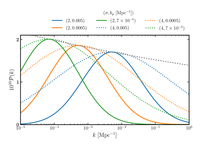
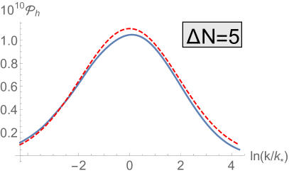
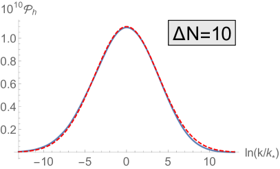
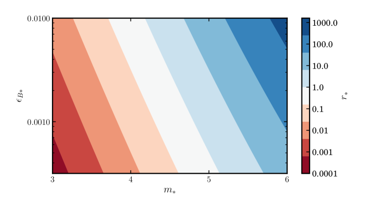
where the amplitude is parameterized by the tensor-to-scalar ratio at the peak scale , is the width of the Gaussian-shaped spectrum, and is the power spectrum of curvature perturbations. We treat and as free parameters in our analysis, while they can be rewritten in terms of more fundamental parameters and , as discussed in Appendix A. Note that, there is no theoretical bound on , while the possible values of are restricted by as Eq. (35). Figure 12 gives an example of how the amplitude is degenerate in and , and we show an example plot of for three sets of these parameters in Figure 1.
Here we define the power spectrum of primordial tensor perturbations to be:
| (3) |
where refers to the circular polarization of the gravitational wave with the momentum vector . For the rest of this paper we model the primordial tensor spectrum as being the sum of two contributions: a completely polarized sourced contribution to the tensor spectrum : and a contribution from the vacuum fluctuations, which we take to be unpolarized and which we do not vary:
| (4) | ||||
where are taken from the best-fit Planck cosmology Planck Collaboration et al. (2016c). We fix which corresponds to the inflationary Hubble scale GeV and the tensor tilt is given by the consistency relation . Note that is not required to be so small compared to the sourced contribution; for larger values of the chiral contribution would be more difficult to detect on the CMB due to the vacuum contribution to the BB spectrum. Therefore , we make the simplifying assumption of a small . In summary:
It is found that contrary to the tensor perturbation, the scalar perturbations in the axion-SU(2) sector do not have any instability for and they are even suppressed compared to the vacuum fluctuation of a massless scalar field due to their kinetic and mass mixing Dimastrogiovanni et al. (2017); Adshead et al. (2013); Dimastrogiovanni and Peloso (2013). Since the axion- sector is decoupled from the inflaton and its energy density is subdominant, its contribution to the curvature perturbation is negligible. It is possible that the energy fraction of the axion grows after inflation and becomes a curvaton if is very large and the decay of the axion is suppressed more than that of the inflaton Moroi and Takahashi (2002); Lyth and Wands (2002); Enqvist and Sloth (2002). In that case, the contribution from the scalar perturbations in the axion-SU(2) sector to the curvature perturbation may be significant and hence it would be interesting to investigate such cases. However, it is beyond the scope of this paper. Therefore, we can simply consider that the curvature perturbation produced by the inflaton is not affected by the axion and the SU(2) gauge fields in this model. We may then take the TT, EE, and TE spectra to be given by constrained cosmological parameters (which we take to be: , , , , , ), and investigate only the B-mode spectra: TB, EB, and BB.
III CMB
In this section, we study the CMB phenomenology of the model introduced in §II. The interesting CMB features of this are the non-zero TB and EB spectra produced by the chiral tensor spectrum. We will calculate the expected TB and EB spectra and make forecasts of their detectability by the LiteBIRD satellite in the presence of cosmic-variance, residual foregrounds, instrumental noise, gravitational lensing, and polarimeter self-calibration.
The anisotropies on the CMB are calculated by the integration of the primordial perturbation spectra over the transfer functions describing the evolution of perturbations with time. The tensor contribution to the angular power spectra of the anisotropies are Lue et al. (1999); Saito et al. (2007); Gluscevic and Kamionkowski (2010); Gerbino et al. (2016)
| (5) | ||||
where and , and indicates the tensor transfer function Pritchard and Kamionkowski (2005). To calculate these spectra we use the CLASS code Blas et al. (2011), making the necessary modifications for it to calculate TB and EB spectra. In Figure 2 we plot examples of the BB and TB spectra calculated in this way for a few different combinations of the model parameters, and compare them to the noise contributions from lensing, instrument noise and foreground residuals that we will consider later.
In this paper we assess the detectability of the chirality of the primordial GWB over the parameter space spanned by . Therefore, we calculate the expected signal-to-noise of the combined TB and EB spectra Shiraishi et al. (2016):
| (6) |
where , and is the covariance of our estimate of the power spectra given a certain theoretical and experimental setup: , where tildes indicate the observed spectrum: , with denoting the noise spectrum, and the calculation of is detailed in Appendix B. denotes the highest multipole we consider, which in this case is 500.
Similarly, we can calculate the detectability of the primordial GWB, as opposed to its chirality, by calculating the signal-to-noise of its contribution to the BB spectrum. In the case of no lensing, this is simply:
| (7) |
However, one of the major sources of uncertainty in a measurement of the BB spectrum is due to gravitational lensing. As the CMB propagates to us from the surface of last scattering it is gravitationally lensed by the intervening matter density, converting primary E-mode anisotropies to secondary B-mode anisotropies, which then need to be accounted for in measurements of BB Zaldarriaga and Seljak (1998).
We can separate the contributions to BB into , where ‘Prim’, ‘Lens’ refer to the primordial and lensed contributions respectively. We are interested in measuring , and in effect acts as an extra source of noise, with an unknown amplitude. The modification required to calculate the signal-to-noise of the primordial BB signal is to consider the matrix:
| (8) |
such that:
| (9) |
where the indices run pver ‘Prim’, ‘Lens’. Note that we will assume that the temperature spectrum is perfectly known over the range of scales we are interested in, and that the sourced contribution to the scalar spectrum is negligible Dimastrogiovanni et al. (2017): .
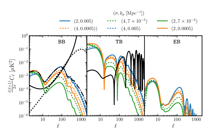
Right panel: (solid colour) and (dashed colour) spectra for the same three sets of parameters. Shown in black is an example of the spurious TB signal induced by polarimeter miscalibration for an angle of one arcminute, as discussed in §III.3.
III.1 Cosmic-variance limited case
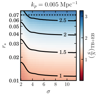
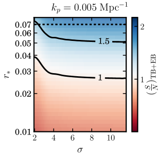
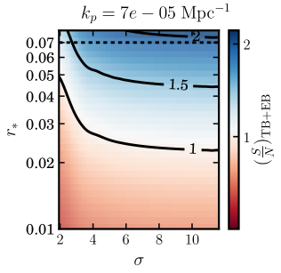
Here, we discuss the signal-to-noise of the TB, EB, and BB spectra in the case of cosmic variance-limited observations: . In this scenario, in the absence of lensing, Equation 7 has the simple analytic form . The signal-to-noise of the TB and EB spectra calculated using Equation 6 are shown in Figure 3 for the parameter space of the model, assuming a lensed BB spectrum with . We consider only , in line with current observational constraints on the scale-invariant tensor-to-scalar ratio , where the subscript indicates the pivot scale in BICEP2 Collaboration et al. (2016). Figure 2 demonstrates that the shape of is strongly dependent on the position of the peak in the GW spectrum, , and also on the width of the peak, . Therefore, the BKP bound on does not simply imply the same bound on ; a small value of and could allow a large value of without exceeding the BKP limit, due to the small scale damping of . However, excepting underestimation for small , the BKP bound provides a useful guide as to what is allowed by current observations.
The values of and were chosen as they probe different scales to which the CMB is sensitive. is more sharply peaked for smaller and so for a given the signal-to-noise decreases with decreasing . As increases the tensor spectrum becomes almost scale-invariant over the range of scales accessible with the CMB and so the signal-to-noise does not depend on for large values of . Figure 3 shows that the maximum achievable signal-to-noise is and that the chirality is undetectable with for .

III.2 Including instrument noise and foreground contamination
We now consider instrument noise, contamination of the spectrum due to imperfect
foreground separation, and assume that we are unable to perform
any ‘delensing’.
The model we use for the noise spectrum includes the instrument noise in the CMB channels, the residual foregrounds in the final CMB map (assumed to be at a level of 2 %, following Refs. Matsumura et al. (2014); Katayama and Komatsu (2011); Shiraishi et al. (2016); Oyama et al. (2016)) and the instrumental noise from channels used for foreground cleaning that is introduced into the CMB channels by the cleaning process. The details of how we combine these factors to produce a final noise contribution to the measured CMB spectrum, as well as the instrument specifications for LiteBIRD can be found in Appendix C. In the left panel of Figure 2 we show the contributions to the BB noise spectrum, , from lensing, LiteBIRD instrumental noise, and foreground residuals compared to the primordial .
III.2.1 BB Signal-to-Noise
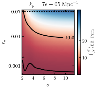
We calculate Equation 9 over the available parameter space and show the result in Figure 4. In a similar way to the TB and EB signal-to-noise we see that there is some dependence on , especially in the case of smaller . This is expected since is slightly smaller than those scales to which we expect the CMB to be sensitive Garcia-Bellido et al. (2016). Therefore, we expect that reducing for this value of will eventually exclude the tensor perturbations from contributing to CMB scales, explaining the sharp decrease in S/N for low and a given . From Figure 4 it is clear that we can detect the primordial contribution to BB for , which is consistent with the aim of LiteBIRD to achieve an uncertainty on the null case of of less than .

III.2.2 TB+EB Signal-to-Noise
Lensing affects the TB and EB signal-to-noise only through , since the direct lensing contributions to TB and EB are negligible Saito et al. (2007); Shiraishi et al. (2016). We calculate Equation 6 over the available parameter space, now including instrument noise for a LiteBIRD-type experiment (with parameters shown in Table 2), foreground residuals, and gravitational lensing, and show the result in Figure 5. Over the allowed parameter space, the maximum achievable signal-to-noise is . Whilst for LiteBIRD can not detect chirality in this model, compared to in the CV-limited case. The right panel of Figure 2 demonstrates that the TB and EB signal peaks at , making the large scale foreground residual contribution to the noise, shown in the left panel of Figure 2, the dominant factor causing this reduction in sensitivity.
Improvements in foreground cleaning algorithms could reduce the level of foreground contamination, and perhaps allow a larger sky fraction to be used in the analysis. However, even with perfect control of these factors, the cosmic-variance limit of Figure 3 can not be beaten. We conclude from this study that the most important factor limiting the sensitivity of CMB observations to the chirality of the GWB is the large cosmic variance of the TB and EB spectra due to large scalar T and E signals, respectively.
III.3 Simultaneous detection and self-calibration
In order to achieve its baseline performance target,
LiteBIRD will require an uncertainty on the polarimeter calibration angle of
less than one arcminute O’Dea et al. (2007); Shimon et al. (2008).
There are several methods that have been used in the past
to calibrate polarimeters such as polarized astrophysical
sources like the Crab Nebula (Tau A), or
man-made sources such as a polarization selective mesh.
There are many factors preventing such methods achieving calibrations
better than one degree.
For example, Tau A is the best candidate for a point-like polarized
source, but this provides a calibration uncertainty of degrees
Kaufman et al. (2014), and with these it is hard to achieve a calibration uncertainty
better than one degree Planck Collaboration
et al. (2016d). The polarization
of Tau A also has a poorly understood frequency dependence, and is
ultimately an extended source, making it poorly suited to a characterization
of the polarized beam Nati et al. (2017).
Man-made sources on the other hand must often be placed in the near
field and are unstable over long time frames. However, a recent
proposal of a balloon-borne artificial polarization source
in the far field of ground-based experiments may ameliorate
this problem for ground-based telescopes Nati et al. (2017).
LiteBIRD plans to self-calibrate its polarimeter using the EB spectrum, which
is assumed to have zero contribution from primordial perturbations
Keating et al. (2013). Unfortunately this makes assumptions about cosmology, and uses part
of the constraining power to calibrate the instrument, instead of for
science. Furthermore, residual foreground
contributions to TB and EB may result in a biasing of the calibration
angle. Ref. Abitbol et al. (2016) shows that a miscalibration
angle of 0.5 degrees can result in a bias in the recovered
value of of , which is significant for
LiteBIRD’s aim to push constraints on to .
However, Ref. Abitbol et al. (2016) also finds that TB and EB
are consistent with zero in a study of the low-foreground
BICEP2 region. Furthermore, in a study of the Planck data
Ref. Planck Collaboration
et al. (2016e) finds that
TB and EB are both consistent with zero for sky fractions up to
, and that TB increases to significant
levels only for larger sky fractions, whilst EB is only marginally
non-zero for . Therefore whilst foregrounds must be
considered, they do not necessarily limit the use of this approach to
calibration.
We want to study the detectability of primordial TB and EB correlations when taking self-calibration into account. The self-calibration process is carried out by zeroing the miscalibration by measuring its contribution to the TB and EB spectra. In this analysis we will assume that residual foreground contributions to TB and EB are negligible.
If the angle of the polarimeter is miscalibrated by some angle the measured will be rotated. We work with the spin-2 quantities which have the transformation properties under rotation:
E and B can be computed to find:
which give the resulting rotations of the angular power spectra:
| (10) |
We then replace the primordial spectra in our expression for with the rotated spectra:
We jointly estimate the uncertainty on the miscalibration angle and the recovered amplitude of the TB and EB spectra parametrized by using the Fisher information:
| (11) |
where . The uncertainty on the miscalibration angle is then given by . We can easily calculate the derivatives with respect to in Equation 11 using Equation 10. In order to calculate the derivatives with respect to we write: . In order to study the interaction of the miscalibration angle and primordial chirality we calculate the correlation coefficient:
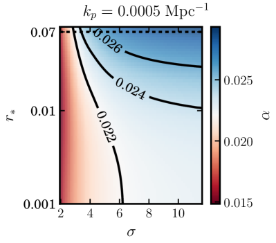
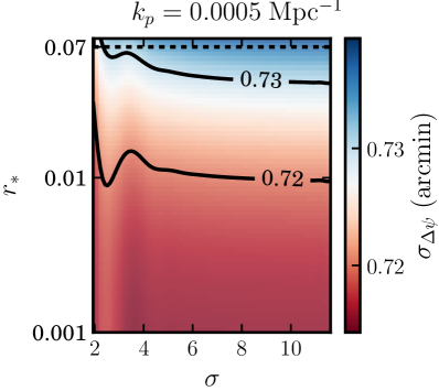
We now calculate the 1-sigma uncertainty in
a measurement of the miscalibration angle and
over the allowed parameter space of the model and show the resulting
contour plots in Figure 6.
We find that for LiteBIRD arcmin for all of the allowed space, making the simultaneous calibration of the polarimeter and detection of the parity-violation possible. The correlation coefficient is less than 0.03 for the allowed parameter space, indicating that the effects of primordial parity-violation and miscalibration are easily separable. This can be understood from the right panel of Figure 2 where it is clear that the primordial signal is a large scale effect, with maximum signal at , whereas the contribution to TB from miscalibration is a small scale effect which dominates at . This is supported by the dependence of in the left panel of Figure 6. The two effects become more correlated for larger values of which correspond to flatter spectra, and hence more power at small scales. Varying has little effect on the result that the effects are separable, but does introduce some interesting dependence on . This indicates that a sufficiently high is necessary for the separation of these effects. For smaller values of , becomes more dependent on . For example, with , for a given , increases with since the flatter spectra of large become more important when is further away from the small scales at which the miscalibration effect occurs. On the other hand when the dependence on is reversed. This is because the miscalibartion effect peaks at , which corresponds to contributions from modes around , where is the comoving distance to the surface of last scattering. Therefore an increase of for will make the signals less correlated as the flatter spectra will introduce more power at larger scales.
In conclusion, any reduction in sensitivity to TB and EB due to the calibration requirements is negligible, and is ignored in the results we quote for LiteBIRD. Our results are in agreement with Refs Ferté and Grain (2014); Gluscevic and Kamionkowski (2010), which also find that the primordial and miscalibration contributions are readily separable.
III.4 CMB Results
Here, we summarize the findings of the CMB section and provide a prognosis of the usefulness of CMB observations in detecting gravitational wave chirality.
In the case of cosmic variance-limited ultimate observations we found
that over the parameter space of the model the maximum signal-to-noise achievable was for the largest values of ,
and that the chirality is undetectable for ,
in agreement with previous studies of simpler models of chiral
GWBs with nearly scale-invariant spectra
Gluscevic and
Kamionkowski (2010); Gerbino et al. (2016); Saito et al. (2007).
Moving on to the realistic case of a LiteBIRD-like experiment with
no delensing capability, a 2% level of foreground residuals,
and a simultaneous self-calibration,
we find that for the largest allowable values of it
may achieve a signal-to-noise of 2.0, making the chirality
detectable. The chirality is undetectable by LiteBIRD
for .
Though a detection with a two sigma significance may be of interest, it
is only achievable for a small part of the parameter space, , and in any event we have demonstrated that we may not
exceed a of 3 using CMB two-point statistics. We also investigated
a COrE+ design with the same level of foreground residuals as LiteBIRD and found
that is performed very similarly to LiteBIRD since both instruments would be
limited by foreground residuals on the large scales we are interested
in. As stated in §I we will not gain anything extra from Stage 4
observations, as they are limited to .
Therefore, in order to make stronger statistical detections of this model
using the CMB, higher order statistical techniques taking advantage of the
model’s non-Gaussianity may have more success as shown for the axion-U(1) model Shiraishi et al. (2016).
Alternatively, we can investigate different physical probes altogether. In the next section, we consider complementary constraints on the axion-SU(2) model from space-based laser interferometer gravitational wave observatories.
IV Laser Interferometers
Due to the strong scale-dependence of the tensor spectrum, it may be possible to study the case of large using laser interferometer gravitational wave observatories. Previous studies have indicated that the scale-invariant spectrum of single-field slow-roll inflation would be too weak at interferometer scales to be detected by current generation interferometers such as LIGO Abbott et al. (2009), VIRGO Accadia et al. (2012), and LISA Bartolo et al. (2016). However, the model we consider has a large feature at , therefore for , current generation interferometers may be sensitive to the GWB of the axion-SU(2) model.
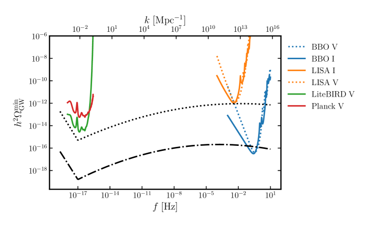
It should be noted that it is difficult to have a sourced gravitational wave spectrum with a sharp peak on interferometer scales. This is because of the attractor behaviour of the background axion field coupled to the SU(2) gauge fields (see Appendix A). As a result, we consider the rather flat spectra seen in Figure 7. For such flat spectra one may expect any signal detectable with interferometers would also be detectable on CMB scales, making the use of interferometers redundant. We therefore first demonstrate the complementarity of our CMB and interferometer studies. We compare their sensitivities as a function of the frequency of the gravitational wave background. The quantity we use to compare sensitivities is the minimum detectable fractional energy density in primordial gravitational waves today:
| (12) |
where is the critical density to close the Universe evaluated today, and , where . The calculation for the CMB is detailed in Appendix D, and for interferometers in the remainder of this section. Figure 7 displays the minimum detectable fractional energy density using the CMB and interferometers for Planck, LiteBIRD, an advanced LISA Bartolo et al. (2016)and BBO Crowder and Cornish (2005). We see that LiteBIRD has a much improved sensitivity to chirality, compared to Planck, which is due to its much lower instrumental noise. The two plotted theoretical spectra are clearly detectable by LISA or BBO, without being detectable at CMB scales, making interferometers an independent, complementary probe of the primordial spectrum of the axion-SU(2) model.
IV.1 Interferometer notation
Laser interferometers consist of a set of test masses placed at nodes and linked by laser beams. Interferometry is used to measure the change in the optical path length between test masses. A passing gravitational wave induces a time-dependent oscillation in the optical path length, which can be isolated from noise by taking cross-correlations between detectors.
The metric perturbation at point at time , , can be decomposed into a superposition of plane waves Allen (1997):
where we use the transverse traceless basis tensors with normalization , and . It is more convenient to deal with complex values, and so we rewrite this as:
where , , and is a unit vector in the direction of propagation of the gravitational wave. Since the coefficients satisfy , is explicitly real. The theory we are dealing with produces a highly non-Gaussian GWB Agrawal et al. (in prep.). We can summarize the two-point statistics using the following expectation values of the Fourier coefficients, but this will not capture all the available information:
| (13) | ||||
where and are the Stokes parameters for intensity and circular polarization respectively. As shown below, quantifies the difference between the amplitudes of two circular polarization states and hence is a clean observable for the chiral GWB Seto (2007); Seto and Taruya (2007, 2008).
IV.2 Interferometer response
In this section, we present the design of the interferometers for which we will forecast the sensitivity to a polarized gravitational wave background. This analysis uses the designs proposed by Ref. Smith and Caldwell (2016). We summarise some of the results of Ref. Smith and Caldwell (2016) here, however for further details we refer readers to Ref. Smith and Caldwell (2016).
Let us consider a set of masses placed at positions , and the phase change, , of light as it travels from mass at time to mass arriving at time Finn (2009):
| (14) |
where is the single-arm transfer function which contains all the geometric information about the instrument and must be derived individually for each interferometer set-up Cornish (2001), and is a unit vector pointing from detector to detector . We now define the Fourier transform of a signal observed for a time : . The Fourier transform of the phase change is then:
| (15) |
where is a finite-time approximation to the delta function defined as , with the properties: , . We may form a signal by constructing a linear combination of phase changes along different paths around the instrument, and then cross-correlating these signals. The signal we seek to measure is stochastic and so to distinguish it from noise we must cross-correlate the detector output with the output from a detector with independent noise properties. The expectation of the cross correlated signal will be composed of terms like:
| (16) |
Using , and we can write this as:
| (17) | ||||
is referred to as the response function of the detector. depends on the relative position and orientation of the arms and , as well as the transfer functions of the two arms.
In the remainder of this section we consider two interferometer designs. In §IV.2.1 we consider the baseline design for near-future space-based interferometers such as the European Space Agency-led Laser Interferometer Space Antenna (LISA) Amaro-Seoane et al. (2013), and in §IV.2.2 we consider two futuristic ‘advanced stage’ LISA-like missions similar to the proposed Big Bang Observatory (BBO) Crowder and Cornish (2005).
IV.2.1 One constellation
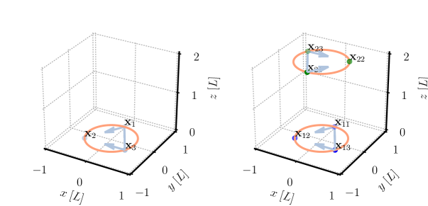
In this section, we consider the design shown in the left panel of Figure 8. This is the baseline design of the LISA mission, and consists of three satellites placed at the vertices of an equilateral triangle of side , and a total of six laser links between the satellites, allowing for measurement of the phase change where . We define the following three signals:
| (18) | ||||
The equilateral design means that the laser phase noise, which is the dominant contribution to the noise terms , cancels Cornish (2001). Furthermore Ref. Smith and Caldwell (2016) shows that signals and have independent noise properties. We therefore consider their cross-correlations:
| (19) |
where , and:
| (20) | ||||
and Cornish (2001); Smith and Caldwell (2016); Romano and Cornish (2016):
Consider the instrument’s response to a gravitational wave travelling in the direction , and another travelling in a direction with , i.e. reflected in the plane. Since the vectors are all in the plane it is easy to see that the products etc. are invariant. Under this transformation only the part of the basis tensor is altered. Since is non-zero only in the part, then the product is invariant. On the other hand the part of the tensor changes sign, meaning that changes sign. Therefore, when performing the angular integral in Equation 20 the terms with a single power of go to zero, giving . The conclusion is that co-planar detectors are not sensitive to the circular polarization of the gravitational wave background. This is true of other types of detectors with planar geometries such as pulsar timing arrays and individual ground-based detectors such as LIGO Abbott et al. (2009).
To gain sensitivity to circular polarization we need to introduce non-co-planar detector arms. Others Seto and Taruya (2007) have considered using cross-correlations between ground-based detectors like LIGO, VIRGO Accadia et al. (2012), and KAGRA Somiya (2012), which have a suitable geometry. In the next subsection we consider an extension to LISA in which we add a second constellation of three satellites to break the co-planar geometry.
IV.2.2 Two-constellations
The extended LISA set-up is shown in the right panel of Figure 8. It consists of two constellations of three equal-arm detectors. The two constellations are separated by a rotation of radians and a translation of . The detector on the constellation is at position , and the unit vectors joining them are given by: . We base this analysis on the designs proposed by Ref. Smith and Caldwell (2016) which optimize the parameters and to achieve equal sensitivity to intensity and polarization of the gravitational wave background. Similar designs have also been considered by Cornish (2001); Crowder and Cornish (2005); Cornish and Larson (2001).
We use the signals defined in Equation 18, but are now written where refers to the constellation on which we are measuring the signal. The detector transfer functions are the same as the single-constellation , but with extra indices referring to the constellation we are considering Cornish (2001); Smith and Caldwell (2016):
| (21) | ||||
Following Smith and Caldwell (2016) we then combine Equations 18 to form estimators sensitive to just intensity or circular polarization:
| (22) | ||||
We will consider two experimental configurations of the two-constellation , introduced in Ref. Smith and Caldwell (2016): ‘LISA’ with , and ‘BBO’ with . These designs are optimized to achieve roughly equal sensitivity to and .
IV.3 Interferometer signal-to-noise
Under the assumption that the signals we are cross-correlating have independent noise properties and are Gaussian-distributed, and that the noise spectrum dominates over the signal, then the signal-to-noise in the interferometer is given by Smith and Caldwell (2016); Cornish (2001); Romano and Cornish (2016):
| (23) |
where is the power spectrum of the noise in the signals, and is the fractional energy
density of gravitational waves in intensity and circular polarization
today, defined in Equation 12. To find the background
fractional energy density today we multiply the primordial spectrum
by the appropriate transfer function
Barnaby et al. (2012); Garcia-Bellido
et al. (2016); Boyle and
Steinhardt (2008):
, where is the fractional energy density
in radiation today.
Up to this point we have not discussed the noise, since it vanishes in the cross-correlations we consider. However it still contributes to the variance of the estimators in Equations 22. There are three major sources of noise in measurements of a particular optical path through an interferometer: shot noise , accelerometer noise , and the dominant laser phase noise, . As pointed out in §IV.2 the major motivation for using equal-arm Michelson interferometers, as given in the first two lines of Equations 18, is the cancellation of the laser phase noise. The shot and acceleration noises can be approximated by taking the fiducial LISA Amaro-Seoane et al. (2013) and BBO Crowder and Cornish (2005) values and scaling them to an instrument with arm length observing at frequency Cornish (2001). The final expressions for are derived by Ref. Smith and Caldwell (2016):
| (24) | ||||
where the values for and for LISA and BBO are given in Ref. Smith and Caldwell (2016). As is the case for the CMB, our Galaxy contains sources of gravitational waves that may act as a confusion noise to a measurement of the GWB Farmer and Phinney (2003); Sathyaprakash and Schutz (2009). It is expected that compact binary systems in our Galaxy will form a gravitational wave foreground with an amplitude in intensity of in the mHz regime. The shape of this spectrum is quite complicated because different periods of a binary system’s evolution dominate at different frequencies and have different frequency dependences Farmer and Phinney (2003). For the design of LISA we consider we expect the impact of such a foreground to be small compared to the acceleration noise Klein et al. (2016). The BBO design we consider peaks at Hz, which is expected to be relatively free of such sources of noise Ferrari et al. (1999); Ungarelli and Vecchio (2001). However, we are mainly interested in detecting chirality of the GWB, and this is more easily distinguished from astrophysical foregrounds, and accordingly previous studies have not considered polarised foregrounds Smith and Caldwell (2016); Seto (2007); Garcia-Bellido et al. (2016). Therefore, we do not consider a contribution to the noise from astrophysical foregrounds in intensity or in polarisation, but it should be noted that we expect a small degradation in the achievable intensity sensitivity of the fiducial LISA design compared to our result, due to the confusion noise of astrophysical sources.
IV.4 Interferometer results


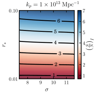
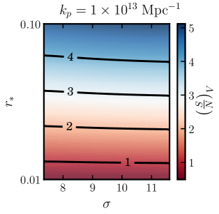
In Figure 9 we plot signal-to-noise contours for LISA assuming and in Figure 10 we plot the corresponding contours for BBO assuming . We see that both the LISA and BBO configurations may detect a polarized gravitational wave background with signal-to-noise greater than one in a regime unavailable to the CMB. In the case of LISA the signal-to-noise for is of order one. However, we see that a BBO-like design far exceeds the sensitivity of LISA, probing a much larger range of for the large values, inaccessible to CMB experiments. A single constellation design described in IV.2.1 would achieve equivalent sensitivity in to LISA and BBO, but with no sensitivity. Therefore, the fiducial LISA design would be sensitive to the inflationary model we consider here, since a positive detection of at these scales with no corresponding detection on CMB scales would require a strong scale dependence of the gravitational wave spectrum.
V Discussion
In this paper we have considered for the first time the detectability of a new model for the production of gravitational waves proposed in Ref. Dimastrogiovanni et al. (2017). Given the increasing effort to measure the B-mode spectrum of the CMB, this is an important step in establishing the origins of any detected primordial tensor perturbations. This model has a unique tensor spectrum characterized by its scale-dependence and chirality, both of which we use in order to find observational markers that allow it to be distinguished from the conventional primordial gravitational waves produced by vacuum fluctuations. If a detection of primordial gravitational waves is made, and the markers we find to be detectable are absent, we may then rule out such a model. In §III we provided robust forecasts of the ability of the LiteBIRD satellite mission to detect the TB and EB correlations that result from the chiral tensor spectrum. We found that LiteBIRD would be able to detect the chirality for , whilst is required by current observations. The addition of Stage 4 observations has little effect as such a survey would be limited to , but the primordial chiral signal is contained almost entirely within . Further, we found that for cosmic-variance limited observations the maximum achievable signal-to-noise for would be . From these studies we conclude that the ability of CMB two-point statistics to determine the presence of a chiral GWB is fairly limited.
However, in this study we have not fully leveraged the scale-dependence of the axion-SU(2) model. Single-field slow-roll expects the tensor spectrum to have a tilt given by the self-consistency relation , and it would be possible to test departures from this using a combination of both CMB and interferometer constraints to provide a lever-arm Meerburg et al. (2015); Lasky et al. (2016). Such a study would be aided by future groundbased observations such as Simons Observatory or S4. In this study we found that for a peak wavenumber in the range the primordial BB spectrum is detectable by LiteBIRD with for . However, the projected sensitivity on for LiteBIRD alone is , which is not sufficient to test deviations from the self-consistency relation, without external constraints.
Another characteristic of the axion-SU(2) model of Ref.
Dimastrogiovanni
et al. (2017) is its intrinsic non-Gaussianity.
Some studies have recently shown that higher order statistics of B-modes,
such as the BBB bispectrum, may yield a significance for the axion-U(1) model Shiraishi et al. (2016); Namba et al. (2016). An analysis of
the CMB non-Gaussianity for the axion-SU(2) model is therefore in order Agrawal et al. (in prep.).
In §IV we showed that interferometers may provide a complementary probe to the CMB at much smaller scales , even for the relatively flat spectra required by the attractor behaviour of the background axion field coupled to the SU(2) gauge field. This takes advantage of the scale-dependence of the axion-SU(2) model, which allows the spectrum to have a large excursion at some scale , e.g. as shown in Figure 7, making the cosmological GWB of the axion-SU(2) model a viable target for interferometers with current sensitivities. We went on to consider two designs of an advanced stage LISA-like mission proposed by Ref. Smith and Caldwell (2016) which are sensitive to both the intensity and circular polarization of the GWB. Whilst interferometers are not in general sensitive to the same parameter space of the model as CMB probes, we found that for spectra with a very large values of and , that would be undetectable on CMB scales, such experiments could make significant detections, and therefore complement CMB constraints.
Acknowledgements.
BT would like to acknowledge the support of the University of Oxford-Kavli IPMU Fellowship and an STFC studentship. MS was supported in part by a Grant-in-Aid for JSPS Research under Grant No. 27-10917 and JSPS Grant-in-Aid for Research Activity Start-up Grant Number 17H07319. The work of TF is partially supported by the JSPS Overseas Research Fellowships, Grant No. 27-154. Numerical computations were in part carried out on Cray XC30 at Center for Computational Astrophysics, National Astronomical Observatory of Japan. We were supported in part by the World Premier International Research Center Initiative (WPI Initiative), MEXT, Japan. TF would like to thank Kavli IPMU for warm hospitality during his stay. This work was supported in part by JSPS KAKENHI Grant Number JP15H05896. MH and NK acknowledge support from MEXT KAKENHI Grant Number JP15H05891.References
- Baumann et al. (2009) D. Baumann, M. G. Jackson, P. Adshead, A. Amblard, A. Ashoorioon, N. Bartolo, R. Bean, M. Beltrán, F. de Bernardis, S. Bird, et al. (2009), vol. 1141 of American Institute of Physics Conference Series, pp. 10–120, eprint 0811.3919.
- Kamionkowski and Kovetz (2016) M. Kamionkowski and E. D. Kovetz, Ann. Rev. Astron. Astrophys. 54, 227 (2016), eprint 1510.06042.
- Guzzetti et al. (2016) C. Guzzetti, M., N. Bartolo, M. Liguori, and S. Matarrese, Riv. Nuovo Cim. 39, 399 (2016), eprint 1605.01615.
- The Polarbear Collaboration: P. A. R. Ade et al. (2014) The Polarbear Collaboration: P. A. R. Ade, Y. Akiba, A. E. Anthony, K. Arnold, M. Atlas, D. Barron, D. Boettger, J. Borrill, S. Chapman, Y. Chinone, et al., Astrophys. J. 794, 171 (2014), eprint 1403.2369.
- Keisler et al. (2015) R. Keisler, S. Hoover, N. Harrington, J. W. Henning, P. A. R. Ade, K. A. Aird, J. E. Austermann, J. A. Beall, A. N. Bender, B. A. Benson, et al., Astrophys. J. 807, 151 (2015), eprint 1503.02315.
- Naess et al. (2014) S. Naess, M. Hasselfield, J. McMahon, M. D. Niemack, G. E. Addison, P. A. R. Ade, R. Allison, M. Amiri, N. Battaglia, J. A. Beall, et al., JCAP 10, 007 (2014), eprint 1405.5524.
- BICEP2 Collaboration et al. (2016) BICEP2 Collaboration, Keck Array Collaboration, P. A. R. Ade, Z. Ahmed, R. W. Aikin, K. D. Alexander, D. Barkats, S. J. Benton, C. A. Bischoff, J. J. Bock, et al., Physical Review Letters 116, 031302 (2016), eprint 1510.09217.
- Planck Collaboration et al. (2016a) Planck Collaboration, P. A. R. Ade, N. Aghanim, M. Arnaud, F. Arroja, M. Ashdown, J. Aumont, C. Baccigalupi, M. Ballardini, A. J. Banday, et al., A&A 594, A20 (2016a), eprint 1502.02114.
- Hazumi et al. (2012) M. Hazumi et al. (LiteBIRD), Proc. SPIE Int. Soc. Opt. Eng. 8442, 844219 (2012).
- de Bernardis (2015) P. de Bernardis, Core+ proposal, http://coresat.planck.fr/uploads/Mission/COrEplus_proposal.pdf (2015), [Online; accessed 27-October-2016].
- Abazajian et al. (2016) K. N. Abazajian, P. Adshead, Z. Ahmed, S. W. Allen, D. Alonso, K. S. Arnold, C. Baccigalupi, J. G. Bartlett, N. Battaglia, B. A. Benson, et al., ArXiv e-prints (2016), eprint 1610.02743.
- Namba et al. (2016) R. Namba, M. Peloso, M. Shiraishi, L. Sorbo, and C. Unal, JCAP 1, 041 (2016), eprint 1509.07521.
- Dimastrogiovanni et al. (2017) E. Dimastrogiovanni, M. Fasiello, and T. Fujita, JCAP 1, 019 (2017), eprint 1608.04216.
- Obata et al. (2016) I. Obata, J. Soda, and CLEO Collaboration, Phys. Rev. D 93, 123502 (2016), eprint 1602.06024.
- Ferreira et al. (2016) R. Z. Ferreira, J. Ganc, J. Noreña, and M. S. Sloth, JCAP 4, 039 (2016), eprint 1512.06116.
- Caprini and Sorbo (2014) C. Caprini and L. Sorbo, JCAP 10, 056 (2014), eprint 1407.2809.
- Mukohyama et al. (2014) S. Mukohyama, R. Namba, M. Peloso, and G. Shiu, JCAP 8, 036 (2014), eprint 1405.0346.
- Peloso et al. (2016) M. Peloso, L. Sorbo, and C. Unal, JCAP 9, 001 (2016), eprint 1606.00459.
- Shiraishi et al. (2016) M. Shiraishi, C. Hikage, R. Namba, T. Namikawa, and M. Hazumi, Phys. Rev. D 94, 043506 (2016), eprint 1606.06082.
- Garcia-Bellido et al. (2016) J. Garcia-Bellido, M. Peloso, and C. Unal, ArXiv e-prints (2016), eprint 1610.03763.
- Lue et al. (1999) A. Lue, L.-M. Wang, and M. Kamionkowski, Phys. Rev. Lett. 83, 1506 (1999), eprint astro-ph/9812088.
- Kamionkowski et al. (1997) M. Kamionkowski, A. Kosowsky, and A. Stebbins, Phys. Rev. D 55, 7368 (1997), eprint astro-ph/9611125.
- Zaldarriaga and Seljak (1997) M. Zaldarriaga and U. Seljak, Phys. Rev. D 55, 1830 (1997), eprint astro-ph/9609170.
- Saito et al. (2007) S. Saito, K. Ichiki, and A. Taruya, JCAP 9, 002 (2007), eprint 0705.3701.
- Gluscevic and Kamionkowski (2010) V. Gluscevic and M. Kamionkowski, Phys. Rev. D 81, 123529 (2010), eprint 1002.1308.
- Gerbino et al. (2016) M. Gerbino, A. Gruppuso, P. Natoli, M. Shiraishi, and A. Melchiorri, JCAP 7, 044 (2016), eprint 1605.09357.
- Planck Collaboration et al. (2016b) Planck Collaboration, N. Aghanim, M. Ashdown, J. Aumont, C. Baccigalupi, M. Ballardini, A. J. Banday, R. B. Barreiro, N. Bartolo, S. Basak, et al., A&A 596, A110 (2016b), eprint 1605.08633.
- Gruppuso et al. (2016) A. Gruppuso, M. Gerbino, P. Natoli, L. Pagano, N. Mandolesi, A. Melchiorri, and D. Molinari, JCAP 6, 001 (2016), eprint 1509.04157.
- Molinari et al. (2016) D. Molinari, A. Gruppuso, and P. Natoli, Physics of the Dark Universe 14, 65 (2016), eprint 1605.01667.
- Seto (2007) N. Seto, Phys. Rev. D75, 061302 (2007), eprint astro-ph/0609633.
- Seto and Taruya (2007) N. Seto and A. Taruya, Physical Review Letters 99, 121101 (2007), eprint 0707.0535.
- Seto and Taruya (2008) N. Seto and A. Taruya, Phys. Rev. D 77, 103001 (2008), eprint 0801.4185.
- Smith and Caldwell (2016) T. L. Smith and R. Caldwell, arXiv preprint arXiv:1609.05901 (2016).
- Matsumura et al. (2014) T. Matsumura, Y. Akiba, J. Borrill, Y. Chinone, M. Dobbs, H. Fuke, A. Ghribi, M. Hasegawa, K. Hattori, M. Hattori, et al., Journal of Low Temperature Physics 176, 733 (2014).
- Matsumura et al. (2016) T. Matsumura et al., Journal of Low Temperature Physics (2016).
- Ferté and Grain (2014) A. Ferté and J. Grain, Phys. Rev. D 89, 103516 (2014), eprint 1404.6660.
- Amaro-Seoane et al. (2013) P. Amaro-Seoane, S. Aoudia, S. Babak, P. Binétruy, E. Berti, A. Bohé, C. Caprini, M. Colpi, N. J. Cornish, K. Danzmann, et al., GW Notes, Vol. 6, p. 4-110 6, 4 (2013), eprint 1201.3621.
- Bartolo et al. (2016) N. Bartolo et al., JCAP 1612, 026 (2016), eprint 1610.06481.
- Planck Collaboration et al. (2016c) Planck Collaboration, P. A. R. Ade, N. Aghanim, M. Arnaud, M. Ashdown, J. Aumont, C. Baccigalupi, A. J. Banday, R. B. Barreiro, J. G. Bartlett, et al., A&A 594, A13 (2016c), eprint 1502.01589.
- Adshead et al. (2013) P. Adshead, E. Martinec, and M. Wyman, Physical Review D 88, 021302 (2013).
- Dimastrogiovanni and Peloso (2013) E. Dimastrogiovanni and M. Peloso, Phys. Rev. D 87, 103501 (2013), eprint 1212.5184.
- Moroi and Takahashi (2002) T. Moroi and T. Takahashi, Phys. Rev. D 66, 063501 (2002), eprint hep-ph/0206026.
- Lyth and Wands (2002) D. H. Lyth and D. Wands, Physics Letters B 524, 5 (2002), eprint hep-ph/0110002.
- Enqvist and Sloth (2002) K. Enqvist and M. S. Sloth, Nuclear Physics B 626, 395 (2002), eprint hep-ph/0109214.
- Pritchard and Kamionkowski (2005) J. R. Pritchard and M. Kamionkowski, Annals Phys. 318, 2 (2005), eprint astro-ph/0412581.
- Blas et al. (2011) D. Blas, J. Lesgourgues, and T. Tram, JCAP 7, 034 (2011), eprint 1104.2933.
- Zaldarriaga and Seljak (1998) M. Zaldarriaga and U. Seljak, Phys. Rev. D 58, 023003 (1998), eprint astro-ph/9803150.
- Katayama and Komatsu (2011) N. Katayama and E. Komatsu, Astrophys. J. 737, 78 (2011), eprint 1101.5210.
- Oyama et al. (2016) Y. Oyama, K. Kohri, and M. Hazumi, JCAP 2, 008 (2016), eprint 1510.03806.
- O’Dea et al. (2007) D. O’Dea, A. Challinor, and B. R. Johnson, MNRAS 376, 1767 (2007), eprint astro-ph/0610361.
- Shimon et al. (2008) M. Shimon, B. Keating, N. Ponthieu, and E. Hivon, Phys. Rev. D 77, 083003 (2008), eprint 0709.1513.
- Kaufman et al. (2014) J. P. Kaufman, N. J. Miller, M. Shimon, D. Barkats, C. Bischoff, I. Buder, B. G. Keating, J. M. Kovac, P. A. R. Ade, R. Aikin, et al., Phys. Rev. D 89, 062006 (2014), eprint 1312.7877.
- Planck Collaboration et al. (2016d) Planck Collaboration, R. Adam, P. A. R. Ade, N. Aghanim, M. Arnaud, M. Ashdown, J. Aumont, C. Baccigalupi, A. J. Banday, R. B. Barreiro, et al., A&A 594, A8 (2016d), eprint 1502.01587.
- Nati et al. (2017) F. Nati, M. J. Devlin, M. Gerbino, B. R. Johnson, B. Keating, L. Pagano, and G. Teply, ArXiv e-prints (2017), eprint 1704.02704.
- Keating et al. (2013) B. G. Keating, M. Shimon, and A. P. S. Yadav, ApJL 762, L23 (2013), eprint 1211.5734.
- Abitbol et al. (2016) M. H. Abitbol, J. C. Hill, and B. R. Johnson, Monthly Notices of the Royal Astronomical Society 457, 1796 (2016), URL http://dx.doi.org/10.1093/mnras/stw030.
- Planck Collaboration et al. (2016e) Planck Collaboration, R. Adam, P. A. R. Ade, N. Aghanim, M. Arnaud, J. Aumont, C. Baccigalupi, A. J. Banday, R. B. Barreiro, J. G. Bartlett, et al., A&A 586, A133 (2016e), eprint 1409.5738.
- Abbott et al. (2009) B. P. Abbott, R. Abbott, R. Adhikari, P. Ajith, B. Allen, G. Allen, R. S. Amin, S. B. Anderson, W. G. Anderson, M. A. Arain, et al., Reports on Progress in Physics 72, 076901 (2009), eprint 0711.3041.
- Accadia et al. (2012) T. Accadia, F. Acernese, M. Alshourbagy, P. Amico, F. Antonucci, S. Aoudia, N. Arnaud, C. Arnault, K. G. Arun, P. Astone, et al., Journal of Instrumentation 7, P03012 (2012), URL http://stacks.iop.org/1748-0221/7/i=03/a=P03012.
- Crowder and Cornish (2005) J. Crowder and N. J. Cornish, Phys. Rev. D 72, 083005 (2005), eprint gr-qc/0506015.
- Allen (1997) B. Allen, in Relativistic Gravitation and Gravitational Radiation, edited by J.-A. Marck and J.-P. Lasota (1997), p. 373, eprint gr-qc/9604033.
- Agrawal et al. (in prep.) A. Agrawal, T. Fujita, and E. Komatsu (in prep.).
- Finn (2009) L. S. Finn, Phys. Rev. D 79, 022002 (2009), eprint 0810.4529.
- Cornish (2001) N. J. Cornish, Phys. Rev. D 65, 022004 (2001), eprint gr-qc/0106058.
- Romano and Cornish (2016) J. D. Romano and N. J. Cornish, ArXiv e-prints (2016), eprint 1608.06889.
- Somiya (2012) K. Somiya, Classical and Quantum Gravity 29, 124007 (2012), eprint 1111.7185.
- Cornish and Larson (2001) N. J. Cornish and S. L. Larson, Classical and Quantum Gravity 18, 3473 (2001), eprint gr-qc/0103075.
- Barnaby et al. (2012) N. Barnaby, J. Moxon, R. Namba, M. Peloso, G. Shiu, and P. Zhou, Phys. Rev. D 86, 103508 (2012), eprint 1206.6117.
- Boyle and Steinhardt (2008) L. A. Boyle and P. J. Steinhardt, Phys. Rev. D 77, 063504 (2008), eprint astro-ph/0512014.
- Farmer and Phinney (2003) A. J. Farmer and E. S. Phinney, MNRAS 346, 1197 (2003), eprint astro-ph/0304393.
- Sathyaprakash and Schutz (2009) B. S. Sathyaprakash and B. F. Schutz, Living Reviews in Relativity 12, 2 (2009), eprint 0903.0338.
- Klein et al. (2016) A. Klein, E. Barausse, A. Sesana, A. Petiteau, E. Berti, S. Babak, J. Gair, S. Aoudia, I. Hinder, F. Ohme, et al., Phys. Rev. D 93, 024003 (2016), eprint 1511.05581.
- Ferrari et al. (1999) V. Ferrari, S. Matarrese, and R. Schneider, MNRAS 303, 247 (1999), eprint astro-ph/9804259.
- Ungarelli and Vecchio (2001) C. Ungarelli and A. Vecchio, Phys. Rev. D 63, 064030 (2001), URL https://link.aps.org/doi/10.1103/PhysRevD.63.064030.
- Seto (2007) N. Seto, Phys. Rev. D 75, 061302 (2007), eprint astro-ph/0609633.
- Meerburg et al. (2015) P. D. Meerburg, R. Hložek, B. Hadzhiyska, and J. Meyers, Phys. Rev. D 91, 103505 (2015), eprint 1502.00302.
- Lasky et al. (2016) P. D. Lasky, C. M. F. Mingarelli, T. L. Smith, J. T. Giblin, E. Thrane, D. J. Reardon, R. Caldwell, M. Bailes, N. D. R. Bhat, S. Burke-Spolaor, et al., Physical Review X 6, 011035 (2016), eprint 1511.05994.
- Watanabe and Komatsu (2006) Y. Watanabe and E. Komatsu, Phys. Rev. D 73, 123515 (2006), eprint astro-ph/0604176.
Appendix A Derivation of the template for GW power spectrum
In Ref.Dimastrogiovanni et al. (2017), it has been shown that the power spectrum of the sourced GW is given by
| (25) |
where is the inflationary Hubble scale, roughly indicates the energy fraction of the SU(2) gauge field. is a monotonically increasing function for which is well approximated by
| (26) |
where the value of a dynamical parameter around the horizon crossing is substituted. Solving the background equations of motion for and with the slow-roll approximation, one can show
| (27) |
where is the maximum value of . From the definition of and , the value of at is . Therefore the tensor-to-scalar ratio on the peak scale of the sourced GW power spectrum is
| (28) |
Next, we consider the width of the GW spectrum. Around the peak of at , or , is expanded as
| (29) |
where , and one can show in the slow-roll regime. Then we obtain the approximated equation for which is valid around the peak value ,
| (30) |
where we define . Substituting it into eq. (25) and using , we obtain the leading order result as
| (31) |
with . Note that the contribution from in the prefactor should not be missed. Comparing it with the template eq. (2), one finds
| (32) |
The validity of the derived expression for is checked by the comparison with the full numerical result. Once and are fixed, all the model parameters and are determined. Then we can numerically solve the background equation of and as well as the equations for the perturbations and to obtain the power spectrum of the sourced GW. In Figure. 11, we compare the derived expression with the full numerical result. It should be noted that eq. (25) and our derivation rely on the slow-roll approximation. The approximation is less accurate for a small , because characterizes the time scale of rolling down its potential. In Figure. 11, one can find a small deviation in the case of , while the excellent agreement is seen for .
Finally, we discuss how long it takes to get to , given that the initial value of is negligibly small compared to . Assuming and using eq. (29), one finds
| (33) |
However, it is definitely underestimated, because must be smaller than which is the maximum value. In fact, a full numerical calculation shows that the coefficient is somewhat larger,
| (34) |
One may wonder if can stay on the top of its potential hill for a longer time if its initial value is small enough. However, since is coupled to the SU(2) gauge fields and the system quickly goes to the attractor behavior, the time scale of the motion of is almost solely determined by . It indicates that the peak scale should be smaller than . Here is the wave number of the mode exiting the horizon at the initial time, and it is smaller or roughly equals to the largest CMB scale. Therefore we obtain the following constraint on ,
| (35) |
Appendix B Calculation of the covariance matrix,
For a given beam, , and a white noise level, , the expected variance of the multipoles of an observed sky is given by:
| (36) |
An unbiased estimator of the angular power spectrum is then:
| (37) |
By considering the expectation it can then be shown that the covariance is given by Gluscevic and Kamionkowski (2010):
| (38) |
where .
Appendix C CMB noise spectrum
For a given set of experimental parameters such as channel frequencies, FWHM and sensitivity in polarization and temperature per channel we want to find the aggregate noise in the CMB spectra. We follow the treatment of Ref. Shiraishi et al. (2016), which itself closely follows Ref. Oyama et al. (2016).
There are multiple sources of noise in the final spectrum: instrumental noise in the CMB channels, residual foreground noise from incomplete cleaning, and additional systematic noise introduced from the templates used in cleaning the CMB channels.
The noise in the final CMB spectrum is:
| (39) |
where the index runs over channels used in CMB analysis, RF refers to residual foregrounds, is the noise spectrum in the channels used for CMB analysis, is the residual foreground level in dust and synchrotron rescaled to the frequencies used in CMB analysis, and is the instrumental uncertainty in the process of foreground removal.
The simplest of the above terms is the noise in the CMB channels:
where is the FWHM of the channel in arcminutes. The instrumental uncertainties in the process of foreground removal are given by Ref. Oyama et al. (2016):
where is the number of channels used in foreground cleaning (in this case ), and are the highest and lowest frequency channel used in the removal (in this case ). The foreground spectra are:
These are converted into a Gaussian addition to the noise by the factor such that a 2% residual level corresponds to .
The spectral parameters of the foreground s are summarized in Table 1. They are taken from Ref. Oyama et al. (2016), and are consistent with the 2015 Planck data.
| Parameter | Value |
|---|---|
| -3 | |
| -2.6 | |
| 30 GHz | |
| 350 | |
| 2.2 | |
| -2.5 | |
| 94 GHz | |
| 10 | |
| 18 K | |
| 0.15 |
| Channel (GHz) | (amin) | |
|---|---|---|
| 40.0 | 69.0 | 36.8 |
| 50.0 | 56.0 | 23.6 |
| 60.0 | 48.0 | 19.5 |
| 68.0 | 43.0 | 15.9 |
| 78.0 | 39.0 | 13.3 |
| 89.0 | 35.0 | 11.5 |
| 100.0 | 29.0 | 9.0 |
| 119.0 | 25.0 | 7.5 |
| 140.0 | 23.0 | 5.8 |
| 166.0 | 21.0 | 6.3 |
| 195.0 | 20.0 | 5.7 |
| 235.0 | 19.0 | 7.5 |
| 280.0 | 24.0 | 13.0 |
| 337.0 | 20.0 | 19.1 |
| 402.0 | 17.0 | 36.9 |
Appendix D Frequency dependence of CMB sensitivity
When we calculate the CMB angular power spectrum we are decomposing the signal into multipoles corresponding to certain angular distance on the sky. Each multipole has contributions from all frequencies of the GWB, determined by an integral of transfer functions:
This makes a direct link between multipole and frequency ambiguous. Since the transfer functions are sharply peaked at with denoting the comoving distance to the last scattering surface. We make the approximation:
| (40) | ||||
To calculate the sensitivity to a circular background we calculate the signal-to-noise of the TB spectrum, ignoring the small contribution from EB for simplicity. The signal-to-noise is therefore:
where over-hat indicates the observed spectrum, including foreground residuals, instrument noise, and lensing. Our assumption that the transfer function is strongly peaked at now allows us to write this as a function of instead of just :
Note that we still calculate the observed spectrum fully. We then ask the question: what is the required (take ) to achieve a signal-to-noise of one in the channel ? This will be the minimum GWB detectable with a signal-to-noise of one. So:
This quantity tells us about the tensor spectrum at recombination, however in order to compare with interferometers which are sensitive to the current GWB, we have to evolve this forward in time. The tensor spectrum transfer function for CMB scales is Smith and Caldwell (2016); Watanabe and Komatsu (2006):
| (41) |