Sensitivity Analysis
for Mirror-Stratifiable Convex Functions

Abstract

This paper provides a set of sensitivity analysis and activity identification results for a class of convex functions with a strong geometric structure, that we coined “mirror-stratifiable”. These functions are such that there is a bijection between a primal and a dual stratification of the space into partitioning sets, called strata. This pairing is crucial to track the strata that are identifiable by solutions of parametrized optimization problems or by iterates of optimization algorithms. This class of functions encompasses all regularizers routinely used in signal and image processing, machine learning, and statistics. We show that this “mirror-stratifiable” structure enjoys a nice sensitivity theory, allowing us to study stability of solutions of optimization problems to small perturbations, as well as activity identification of first-order proximal splitting-type algorithms. Existing results in the literature typically assume that, under a non-degeneracy condition, the active set associated to a minimizer is stable to small perturbations and is identified in finite time by optimization schemes. In contrast, our results do not require any non-degeneracy assumption: in consequence, the optimal active set is not necessarily stable anymore, but we are able to track precisely the set of identifiable strata.We show that these results have crucial implications when solving challenging ill-posed inverse problems via regularization, a typical scenario where the non-degeneracy condition is not fulfilled. Our theoretical results, illustrated by numerical simulations, allow us to characterize the instability behaviour of the regularized solutions, by locating the set of all low-dimensional strata that can be potentially identified by these solutions.

1 Introduction

Variational methods and non-smooth optimization algorithms are ubiquitous to solve large-scale inverse problems in various fields of science and engineering, and in particular in data science. The non-smooth structure of the optimization problems promotes solutions conforming to some notion of simplicity or low-complexity (e.g. sparsity, low-rank, etc.). The low-complexity structure is often manifested in the form of a low-dimensional “active set”. It is thus of prominent interest to be able to quantitatively characterize the stability of these active sets to perturbations of the objective function. Of crucial importance is also the identification in finite time of these active sets by iterates of optimization algorithms that numerically minimize the objective function. This type of problems and results is referred to as “activity identification”; a review of the relevant literature will be provided in the sequel (at the beginning of each section). In a nutshell, the existing identification results guarantee a perfect stability of the active set to perturbations, or a finite identification of this active set via algorithmic schemes, under some non-degeneracy conditions (see in particular [39, 24, 58]). The crucial non-degeneracy assumption, that takes generally the form (10), can be viewed as a geometric generalization of strict complementary in non-linear programming. However, as we will illustrate shortly through some preliminary numerics, such a condition is too stringent and is often barely verified. The goal of this paper is to investigate the situation where this non-degeneracy assumption is violated.

1.1 Motivating Examples

In order to better grasp the relevance of our analysis, let us first start with the setting of inverse problems that pervades various fields including signal processing and machine learning. We will come back to this setting in Section 4 with further discussions and references.

Regularized Inverse Problems

Assume one observes

$$y=\mathring{y}+w\in\mathbb{R}^{P}\quad\text{where}\quad\mathring{y}\stackrel{{\scriptstyle\mbox{\tiny def.}}}{{=}}\Phi\mathring{x}$$ (1)

where $w$ is some perturbation (called noise) and $\Phi\in\mathbb{R}^{P\times N}$ (called forward operator, or design matrix in statistics). Solving an inverse problem amounts to recovering $\mathring{x}$, to a good approximation, knowing $y$ and $\Phi$ according to (1). Unfortunately, in general, $P$ can be much smaller than the ambient dimension $N$, and when $P=N$, the mapping $\Phi$ is in general ill-conditioned or even singular.

A classical approach is then to assume that $\mathring{x}$ has some ”low-complexity”, and to use a prior regularization $R$ promoting solutions with such low-complexity. This leads to the following optimization problem

$$\underset{x\in\mathbb{R}^{N}}{\min}\;E(x,(\lambda,y))\stackrel{{\scriptstyle\mbox{\tiny def.}}}{{=}}R(x)+\frac{1}{2\lambda}|\!|y-\Phi x|\!|^{2}, \mathcal{P}(\lambda,y)$$ ()

Let us discuss two popular examples of regularizing functions promoting a low-complexity structure. These two functions will be used in our numerical experiments.

Example 1 ($\ell_{1}$ norm).

For $x\in\mathbb{R}^{N}$, its $\ell_{1}$ norm reads

$$R(x)=|\!|x|\!|_{1}\stackrel{{\scriptstyle\mbox{\tiny def.}}}{{=}}\sum_{i=1}^{N}|x^{i}|,$$ (2)

where $x^{i}$ is the $i$-th entry of $x$. As advocated for instance by [15, 55], the $\ell_{1}$ enforces the solutions of ($\mathcal{P}(\lambda,y)$) to be sparse, i.e. to have a small number of non-zero components. Indeed, the $\ell_{1}$ norm can be shown to be the tightest convex relaxation (in the sense of bi-conjugation) of the $\ell_{0}$ pseudo-norm restricted to the unit Euclidian ball [37]. Recall that $\ell_{0}$ pseudo-norm of $x\in\mathbb{R}^{N}$ measures its sparsity

$$|\!|x|\!|_{0}\stackrel{{\scriptstyle\mbox{\tiny def.}}}{{=}}\sharp\left\{i\in\{1,\ldots,N\}\;:\;x^{i}\neq 0\right\}.$$

Sparsity has witnessed a huge surge of interest in the last decades. For instance, in signal and imaging sciences, one can approximate most natural signals and images using sparse expansions in an appropriate dictionary (see e.g. [45]). In statistics, sparsity is a key toward model selection and interpretability [9].

Example 2 (Nuclear norm).

For a matrix $x\in\mathbb{R}^{n_{1}\times n_{2}}\sim\mathbb{R}^{N}$, where $N=n_{1}n_{2}$, the nuclear norm is defined as

$$|\!|x|\!|_{*}\stackrel{{\scriptstyle\mbox{\tiny def.}}}{{=}}|\!|\sigma(x)|\!|_{1}=\sum_{i=1}^{n}\sigma^{i}(x),$$

where $n\stackrel{{\scriptstyle\mbox{\tiny def.}}}{{=}}\min(n_{1},n_{2})$ and $\sigma(x)=(\sigma^{1}(x),\ldots,\sigma^{n}(x))\in\mathbb{R}_{+}^{n}$ is the vector of singular values of $x$. The nuclear norm is the tightest convex relaxation of the rank (in the sense of bi-conjugation) restricted to the unit Frobenius ball [36]. This underlies its wide use to promote solutions of ($\mathcal{P}(\lambda,y)$) with low rank, where we recall $\mathop{\operator@font rank}\nolimits(x)\stackrel{{\scriptstyle\mbox{\tiny def.}}}{{=}}|\!|\sigma(x)|\!|_{0}$. Low-rank regularization has proved useful for a variety of applications, including control theory and machine learning; see e.g. [28, 1, 11]

Active set(s) identification

The above discussed regularizers $R$ are non-smooth convex functions. This non-smoothness arises in a highly structured fashion and is usually associated, locally, with some low-dimensional active subset of $\mathbb{R}^{N}$ (in many cases, such a subset is an affine or a smooth manifold). Thus $R$ will favor solutions of ($\mathcal{P}(\lambda,y)$) that lie in a low-dimensional active set and would allow the inversion of the system (1) in a stable way. More precisely, one would like that under small perturbations $w$, the solutions of ($\mathcal{P}(\lambda,y)$) move stably along the active set. A byproduct of this behaviour is that from an algorithmic perspective, if an optimization algorithm is used to solve ($\mathcal{P}(\lambda,y)$), one would hope that the iterates of the scheme identify the active set in finite time.

Identifying the low-dimensional active set in a stable way is highly desirable for several reasons. One reason is that it is a fundamental property most practitioners are looking for. Typical examples include neurosciences [27] where the goal is to recover a spike train from neural activity, or astrophysics [53] where it is desired to separate stars from a background. In both examples, sparsity can be used as a modeling hypothesis and the recovery method should comply with it in a stable way. A second reason is algorithmic since one can also take advantage of the low-dimensionality of the identified active set to reduce computational burden and memory storage, hence opening the door to higher-order acceleration of optimization algorithms (see [38, 46]).

Unfortunately, this desirable behaviour rarely occurs in practical applications. Yet one still observes some form of partial stability (to be given a rigorous meaning in Section 3 and 4), as confirmed by the numerical experiment of the next paragraph.

1.2 Illustrative numerical experiment

We consider a simple “compressed sensing” scenario, with the $\ell_{1}$ norm $R=|\!|\cdot|\!|_{1}$ [12] and the nuclear norm $R=|\!|\cdot|\!|_{*}$ [13] as regularizers. The operator $\Phi\in\mathbb{R}^{N\times P}$ is drawn uniformly at random from the standard Gaussian ensemble, i.e. the entries of $\Phi$ are independent and identically distributed Gaussian random variables with zero-mean and unit variance. In the case $R=|\!|\cdot|\!|_{1}$, we set $(N,P)=(100,50)$ and the vector to recover $\mathring{x}$ is drawn uniformly at random among sparse vectors with $R_{0}(\mathring{x})\stackrel{{\scriptstyle\mbox{\tiny def.}}}{{=}}|\!|\mathring{x}|\!|_{0}=10$ and unit non-zero entries. In the case $R=|\!|\cdot|\!|_{*}$, we set $(N,P)=(400,300)$ ($n_{1}=n_{2}=n=20$) and the matrix to recover $\mathring{x}$ is drawn uniformly at random among low-rank matrices with $R_{0}(\mathring{x})\stackrel{{\scriptstyle\mbox{\tiny def.}}}{{=}}\mathop{\operator@font rank}\nolimits(\mathring{x})=4$ and unit non-zero singular values. For each problem suite $(R,N,P)$, $1000$ realizations of $(\mathring{x},\Phi,w)$ are drawn, and $y$ is then generated according to (1). The entries of the noise vector $w$ are drawn uniformly from a Gaussian with standard deviation $0.1$, we set $\lambda=0.28$ for $R=|\!|\cdot|\!|_{1}$ and $\lambda=10$ for $R=|\!|\cdot|\!|_{*}$.

For each realization of $(\mathring{x},\Phi,w)$, we solve the associated problem ($\mathcal{P}(\lambda,y)$) using CVX [31] to get a high precision; denote $x^{\star}(\lambda,y)$ the obtained solutions. We also solve ($\mathcal{P}(\lambda,y)$) by the Forward-Backward (FB) scheme which reads in this case

$$x_{k+1}=\operatorname{prox}_{\lambda\gamma R}(x_{k}+\gamma\Phi^{*}(y-\Phi x_{k})).$$

In our setting, with $\gamma=1.8/\sigma_{\max}(\Phi^{*}\Phi)$ and non-emptiness of $\operatorname{Argmin}(E(\cdot,\lambda,y)$, it is well-known that the sequence $(x_{k})_{k\in\mathbb{N}}$ converges to a point in $\operatorname{Argmin}(E(\cdot,\lambda,y))$.

The top row of Figure 1 displays the histogram of the complexity index excess ${{\color[rgb]{0,0,0}\delta\stackrel{{\scriptstyle\mbox{\tiny def.}}}{{=}}R_{0}(x^{\star}(\lambda,y))-R_{0}(\mathring{x})}}$ which clearly shows that we do not have exact stability under the perturbations $w$. Indeed, although $R_{0}(x^{\star}(\lambda,y))$ is still rather small, its value is in most cases larger than the complexity index $R_{0}(\mathring{x})$. The bottom row of Figure 1 depicts the evolution with $k$ of the complexity index $R_{0}(x_{k})$ for two random instances of $\mathring{x}$ (in blue and red) corresponding to two different values of ${{\color[rgb]{0,0,0}\delta}}$. One can observe that the iterates identify in finite time some low-dimensional active set with a complexity index strictly larger than the one associated to $\mathring{x}$ (the red curves). We will provide a more detailed discussion of this phenomenon in Section 6.

Histograms of $\delta$
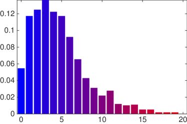
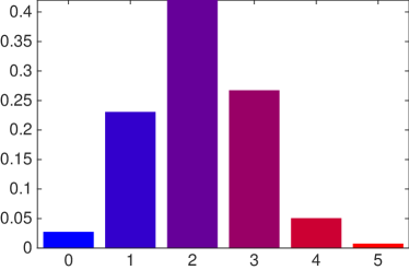
$R_{0}(x_{k})$ vs iteration $k$
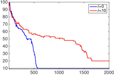
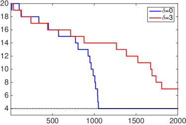
	$R=|\!|\cdot|\!|_{1}$	$R=|\!|\cdot|\!|_{*}$

Fig. 1: Top row: Histogram of the complexity index excess $\delta=R_{0}(x^{\star}(\lambda,y))-R_{0}(\mathring{x})$ where $x^{\star}(\lambda,y)$ is the solution of ($\mathcal{P}(\lambda,y)$) with noisy observation $y=\mathring{y}+w$ for a small perturbation $w$ and a well-chosen parameter value $\lambda=c_{0}|\!|w|\!|$. Bottom row: Evolution of the complexity index $R_{0}(x_{k})$ where $(x_{k})_{k\in\mathbb{N}}$ is the FB iterates sequence converging to some $x^{\star}(\lambda,y)\in\operatorname{Argmin}(E(\cdot,\lambda,y))$.

As we will emphasize in the review of previous work, existing results on sensitivity analysis and low-complexity regularization only focus the case where $R_{0}(x^{\star}(\lambda,y))=R_{0}(\mathring{x})$ (i.e. $\delta=0$), whose underlying claim is that the low-complexity model is perfectly stable to perturbations, which typically requires some non-degeneracy assumption to hold. In many situations, however, including the compressed sensing scenario described above, but also in super-resolution imaging (see [26]) and other challenging inverse problems, non-degeneracy-type hypotheses are too restrictive. It is the goal of this paper to develop a more general sensitivity analysis, that goes beyond the non-degenerate case, to improve our understanding of stability to perturbations of low-complexity regularized inverse problems.

1.3 Contributions and Outline

Our first contribution consists in introducing, in Section 2, a class of proper lower-semicontinuous (lsc) convex functions that we coin “mirror-stratifiable”. The subdifferential of such a function induces a primal-dual pairing of stratifications, which is pivotal to track identifiable strata. We discuss several examples of functions enjoying such a structure. With this structure at hand, we then turn to the main result of this paper, formalized in Theorem 1, and on which all the others rely. This result shows finite enlarged activity identification for a mirror-stratifiable function without the need of any non-degeneracy condition. In addition, the identifiable strata are precisely characterized in terms primal-dual optimal solutions. Sections 3, 4 and 5 instantiate this abstract result for a set of concrete problems, respectively: sensitivity of composite ”smooth+non-smooth” optimization problems (Theorem 2), enlarged activity identification by proximal splitting schemes such as Forward-Backward and Douglas-Rachford algorithms (Theorems 4 and 5), and finally, enlarged identification for regularized inverse problems (Theorem 3). Before stating these results, we make a short review of the associated literature. Finally Section 6 illustrates these theoretical findings with numerical experiments, in particular in a compressed sensing scenario involving the $\ell_{1}$ and nuclear norms as regularizers. Following the philosophy of reproducible research, all the code to reproduce the figures of this article is available online.

2 Mirror-Stratifiable Functions

In this section, we introduce the class of mirror-stratifiable convex functions, and present the sensitivity property they provide (Theorem 1). We also illustrate that many popular regularizers used in data science are mirror-stratifiable. Most the results of this section (in particular all the examples) are easy to obtain by basic calculus; we therefore do not give these proofs in the text and we gather some of them in Appendix A.

2.1 Stratifications and definitions

We start with recalling the following standard definition of stratification.

Definition 1 (Stratification).

A stratification of a set $D\subset\mathbb{R}^{N}$ is a finite partition $\mathcal{M}=\{M_{i}\}_{i\in I}$ such that for any partitioning sets (called strata) $M$ and $M^{\prime}$ we have

$$M\cap\operatorname{cl}(M^{\prime})\neq\emptyset\implies M\subset\operatorname{cl}(M^{\prime}).$$

If the strata are open polyhedra, then $\mathcal{M}$ is a polyhedral stratification, and if they are $C^{2}$-smooth manifolds then $\mathcal{M}$ entails a $C^{2}$-stratification.

A stratification is naturally endowed with the partial ordering $\leqslant$ in the sense that

$$M\leqslant M^{\prime}\quad\Longleftrightarrow\quad M\subset\operatorname{cl}(M^{\prime})\quad\Longleftrightarrow\quad M\cap\operatorname{cl}(M^{\prime})\neq\emptyset.$$ (3)

The relation is clearly reflexive and transitive. Furthermore, we have

$$\operatorname{cl}(M)=\bigcup_{M^{\prime}\leqslant M}M^{\prime}.$$ (4)

An immediate consequence of Definition 1 is that for each point $x\in D$, there is a unique stratum containing $x$, denoted $M_{x}$. Indeed, suppose that there are two non-empty open strata $M_{1}$ and $M_{2}$ such that $M_{1}\cap M_{2}=\{x\}$, and thus $M_{1}\cap M_{2}\neq\emptyset$. This implies, using (3), that $M_{1}\leqslant M_{2}$ and $M_{2}\leqslant M_{1}$, and thus $M_{1}=M_{2}$.

At this stage, it is worth emphasizing that the strata are not needed to be manifolds in the rest of the paper. It is however the case that in many practical cases that we will discuss, strata are indeed manifolds, and sometimes affine manifolds.

Example 3 (Polyhedral sets and functions).

A partition of a polyhedral set into its open faces induces a natural finite polyhedral stratification of it. In turn, let $R:\mathbb{R}^{N}\to\overline{\mathbb{R}}\stackrel{{\scriptstyle\mbox{\tiny def.}}}{{=}}\mathbb{R}\cup\{+\infty\}$ be a polyhedral function, and consider a polyhedral stratification of its epigraph, which is a polyhedral set in $\mathbb{R}^{N+1}$. Projecting all polyhedral strata onto the first $N$-coordinates one obtains a finite polyhedral stratification of $\operatorname{dom}(R)$.

Remark 1.

The previous example extends to semialgebraic sets and functions, which are known to induce stratifications into finite disjoint unions of manifolds. In fact, this holds for any tame class of sets/functions; see, e.g., [18].

We now single out a specific set of strata, called active strata, that will play a central role for finite enlarged activity identification purposes.

Definition 2 (Active strata).

Given a stratification $\mathcal{M}$ of $D\subset\mathbb{R}^{N}$ and a point $x\in D$, a stratum $M\in\mathcal{M}$ is said active at $x$ if $x\in\operatorname{cl}(M)$.

Proposition 1.

Given a stratification $\mathcal{M}$ of $D$ and a point $x\in D$. Then there exists $\delta>0$ such that set of strata $M_{x^{\prime}}$ for any $x^{\prime}$ such that $|\!|x^{\prime}-x|\!|<\delta$, coincides with the set of strata $M\geqslant M_{x}$ and with the set of active strata at $x$.

2.2 Mirror-Stratifiable functions

Following [19, Section 4], we define the key correspondence operator whose role will become apparent shortly.

Definition 3.

Let $R\colon\mathbb{R}^{N}\to\overline{\mathbb{R}}$ be a proper lsc convex function. The associated correspondence operator $\mathcal{J}_{R}:2^{\mathbb{R}^{N}}\to 2^{\mathbb{R}^{N}}$ is defined as

$$\mathcal{J}_{R}(S)\stackrel{{\scriptstyle\mbox{\tiny def.}}}{{=}}\bigcup_{x\in S}\operatorname{ri}(\partial R(x)),$$

where $\partial R$ is the subdifferential of $R$.

Observe that, by definition, $\mathcal{J}_{R}$ is increasing for set inclusion

$$S\subset S^{\prime}\quad\Longrightarrow\quad\mathcal{J}_{R}(S)\subset\mathcal{J}_{R}(S^{\prime}).$$ (5)

For this operator to be useful in sensitivity analysis, we will further impose that $\mathcal{J}_{R}$ is decreasing for the partial ordering $\leqslant$ in (3), as captured in our main definition. This is a key requirement that captures the intuitive idea that the larger a primal stratum, the smaller its image by $\mathcal{J}_{R}$ in the dual space.

In the following, we will denote $R^{*}$ the Legendre-Fenchel conjugate of $R$.

Definition 4 (Mirror-stratifiable functions).

Let $R\colon\mathbb{R}^{N}\to\overline{\mathbb{R}}$ be a proper lsc convex function; we say that $R$ is mirror-stratifiable with respect to a (primal) stratification $\mathcal{M}=\{M_{i}\}_{i\in I}$ of $\operatorname{dom}(\partial R)$ and a (dual) stratification $\mathcal{M}^{*}=\{M^{*}_{i}\}_{i\in I}$ of $\operatorname{dom}(\partial R^{*})$ if the following holds:

1. Conjugation induces a duality pairing between $\mathcal{M}$ and $\mathcal{M}^{*}$, and $\mathcal{J}_{R}:\mathcal{M}\to\mathcal{M}^{*}$ is invertible with inverse $\mathcal{J}_{R^{*}}$, i.e. $\forall M\in\mathcal{M}$, $M^{*}\in\mathcal{M}^{*}$ we have

   $$M^{*}=\mathcal{J}_{R}(M)\iff\mathcal{J}_{R^{*}}(M^{*})=M.$$

2. $\mathcal{J}_{R}$ is decreasing for the relation $\leqslant$: for any $M$ and $M^{\prime}$ in $\mathcal{M}$

   $$M\leqslant M^{\prime}\iff\mathcal{J}_{R}(M)\geqslant\mathcal{J}_{R}(M^{\prime}).$$

The primal-dual stratifications that make $R$ mirror-stratifiable are not unique, as will be exemplified in Remark 3. Though the definition is formal and the assumptions looks restrictive, this class include many useful examples, as illustrated in the next section. We finish this section with a remark, used in the sequel.

Remark 2 (Separability).

For each $m=1,\ldots,L$, suppose that the proper lsc convex function $R_{m}:\mathbb{R}^{N_{m}}\to\overline{\mathbb{R}}$ is mirror-stratifiable with respect to stratifications $\mathcal{M}_{m}$ and $\mathcal{M}_{m}^{*}$. Then it is easy to show, using standard subdifferential and conjugacy calculus, that the function $R:(x_{m})_{1\leqslant m\leqslant L}\in\mathbb{R}^{N_{1}}\times\cdots\times\mathbb{R}^{N_{L}}\mapsto\sum_{m=1}^{L}R_{m}(x_{m})$ is mirror-stratifiable with stratifications $\mathcal{M}_{1}\times\cdots\times\mathcal{M}_{L}$ and $\mathcal{M}_{1}^{*}\times\cdots\times\mathcal{M}_{L}^{*}$.

2.3 Examples

The notion of a mirror-stratifiable function looks quite rigid. However, many of the regularization functions routinely used in data science are mirror-stratifiable. Let us provide some relevant examples in this section. In particular, the $\ell_{1}$-norm and the nuclear norm will be used in the numerical experiments.

2.3.1 Legendre functions

A lsc convex function $R:\mathbb{R}^{N}\to\overline{\mathbb{R}}$ is said to be a Legendre function (see [50, Chapter 26]) if (i) it is differentiable and strictly convex on the interior of its domain $\operatorname{int}(\operatorname{dom}(R))\neq\emptyset$, and (ii) $|\!|\nabla R(x_{k})|\!|\to+\infty$ for every sequence $\left(x_{k}\right)_{k\in\mathbb{N}}\subset\operatorname{int}(\operatorname{dom}(R))$ converging to a boundary point of $\operatorname{dom}(R)$. Many functions in convex optimization are Legendre; most notably, quadratic functions and the log barrier of interior point methods. It was shown in [50, Theorem 26.5] that $R$ is Legendre if and only if its conjugate $R^{*}$ is Legendre, and that in this case $\nabla R$ is a bijection from $\operatorname{int}(\operatorname{dom}(R))$ to $\operatorname{int}(\operatorname{dom}(R^{*}))$ with $\nabla R^{*}=(\nabla R)^{-1}$. As a consequence, a Legendre function $R$ is mirror-stratifiable with $\mathcal{M}=\{\operatorname{int}(\operatorname{dom}(R))\}$ and $\mathcal{M}^{*}=\{\operatorname{int}(\operatorname{dom}(R^{*}))\}$.

2.3.2 $\ell_{1}$-norm

Let $R:x\in\mathbb{R}\mapsto|x|$, whose conjugate $R^{*}=\iota_{[-1,1]}$. It follows that $R$ is mirror-stratifiable with $\mathcal{M}=\left\{\,]-\infty,0[,\{0\},]0,+\infty[\right\}$ and $\mathcal{M}^{*}=\{\{-1\},]-1,1[,\{+1\}\}$. Using Remark 2, the next result is clear.

Lemma 1.

The $\ell_{1}$-norm and its conjugate $\iota_{[-1,+1]^{N}}$ are mirror-stratifiable with respect to the stratifications $\mathcal{M}=\left\{\,]-\infty,0[,\{0\},]0,+\infty[\right\}^{N}$ of $\mathbb{R}^{N}$ and $\mathcal{M}^{*}=\{\{-1\},]-1,1[,\{+1\}\}^{N}$ of $[-1,+1]^{N}$.

A graphical illustration of this lemma in dimension $2$ is displayed in Figure 2(a).

Remark 3 (Non-uniqueness of stratifications).

In general, we do not have uniqueness of stratifications inducing mirror-stratifiable functions. To illustrate this, let us consider the $\ell_{1}$ norm. Take the partitions $\mathcal{M}=\left\{\,]-\infty,0[\cup]0,+\infty[,\{0\}\right\}^{N}$ of $\mathbb{R}^{N}$ and $\mathcal{M}^{*}=\{\{-1,+1\},]-1,1[\}^{N}$. These are valid stratifications though the strata are not connected. Other possible valid stratifications are given by strata $M_{j}=\left\{x\in\mathbb{R}^{N}\;:\;|\!|x|\!|_{0}=j\right\}$ and $M^{*}_{j}=\mathcal{J}_{|\!|\cdot|\!|_{1}}(M_{j})$, for $j=0,1,\ldots,N$. It is immediate to check that the $\ell_{1}$-norm is also mirror-stratifiable with respect to these stratifications. However, as devised above, it is in general not wise to take such large strata as they lead to less sharp localization and sensitivity results.

Remark 4 (Instability under the sum rule).

The family of mirror-stratifiable functions is unfortunately not stable under the sum. As a simple counter-example, consider the pair of conjugate functions on $\mathbb{R}$: $R(x)=|x|+x^{2}/2$ and $R^{*}(u)=(\max\{|u|-1,0\})^{2}/2$. We obviously have $\operatorname{dom}(\partial R)=\operatorname{dom}(\partial R^{*})=\mathbb{R}$. However we observe that $\mathcal{J}_{R}(\mathbb{R})=\mathbb{R}\setminus\{-1,1\}$. This yields that $\mathcal{J}_{R}$ cannot be a pairing between any two stratifications of $\mathbb{R}$, and therefore $R$ cannot be mirror-stratifiable.

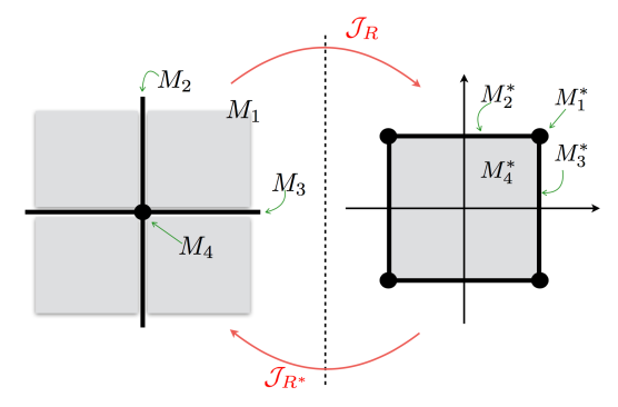
(a)

(b)

Fig. 2: Graphical illustration of mirror-stratification for two norms: (a) $\ell_{1}$ norm in dimension $2$; (b) $\ell_{1,2}$ norm in dimension $3$ (with two blocks, of respectively sizes $1$ and $2$).

2.3.3 $\ell_{1,2}$ norm

The $\ell_{1,2}$ norm, also known as the group Lasso regularization, has been advocated to promote group/block sparsity [60], i.e. it drives all the coefficients in one group to zero together. Let $\mathcal{B}$ a non-overlapping uniform partition of $\{1,\ldots,N\}$ into $K$ blocks. The $\ell_{1,2}$ norm induced by the partition $\mathcal{B}$ reads

$$|\!|x|\!|_{\mathcal{B}}=\sum_{B\in\mathcal{B}}|\!|x^{B}|\!|_{2}$$

where $x^{B}$ is the restriction of $x$ to the entries indexed by the block $B$. This is again a separable function of the $x^{B}$’s. One can easily show that the $\ell_{2}$ norm on $\mathbb{R}^{|B|}$ and its conjugate, the indicator of the unit $\ell_{2}$-ball $\mathbb{B}_{\ell_{2}^{|B|}}$ in $\mathbb{R}^{|B|}$, are mirror-stratifiable with respect to the stratifications $\{\{0\},\mathbb{R}^{|B|}\setminus\{0\}\}$ of $\mathbb{R}^{N}$ and $\{\SS_{\ell_{2}}^{|B|-1},\operatorname{int}(\mathbb{B}_{\ell_{2}^{|B|}})\}$ of $\mathbb{B}_{\ell_{2}^{|B|}})$, where $\SS_{\ell_{2}}^{|B|-1}$ is the corresponding unit sphere. In turn, the $\ell_{1,2}$ norm is mirror-stratifiable with respect to the stratifications $\mathcal{M}=\{\{0\},\mathbb{R}^{|B|}\setminus\{0\}\}^{K}$ and $\mathcal{M}^{*}=\{\SS^{|B|-1},\operatorname{int}(\mathbb{B}_{\ell_{2}^{|B|}})\}^{K}$. An illustration of this result in dimension $3$ is portrayed in Figure 2(b).

2.3.4 Nuclear norm

Let us come back to the nuclear norm defined in Example 2. For simplicity, we assume $n_{1}=n_{2}=n$. Let $M$ be a stratum of the $\ell_{1}$ norm stratification. In the following, we denote by $M^{\operatorname{sym}}$ its symmetrization. We observe that $\sigma^{-1}(M^{\operatorname{sym}})=\left\{X\in\mathbb{R}^{n\times n}\;:\;\mathop{\operator@font rank}\nolimits(X)=|\!|z|\!|_{0},z\in M\right\}$. So many inverse images $\sigma^{-1}(M^{\operatorname{sym}})$ of strata $M^{\operatorname{sym}}$ coincide. This suggests the following $n+1$ stratifications: for a given $i\in\{0,\ldots,N\}$

$$M_{i} = \left\{X\in\mathbb{R}^{n\times n}\;:\;\mathop{\operator@font rank}\nolimits(X)=i\right\}$$

$$M^{*}_{i} = \left\{U\in\mathbb{R}^{n}\;:\;\sigma_{1}(U)=\cdots=\sigma_{i}(U)=1,\forall j>i,\ |\sigma_{j}(U)|<1\right\}.$$

This yields that $|\!|\cdot|\!|_{*}$ is mirror-stratifiable with respect to these stratifications.

2.3.5 Polyhedral Functions

We here establish mirror-stratifiability of polyhedral functions, including the $\ell_{1}$ norm, the $\ell_{\infty}$ norm and anisotropic TV semi-norm.

A polyhedral function $R\colon\mathbb{R}^{N}\to\overline{\mathbb{R}}$ can be expressed as

$$R(x)=\max_{i=1,\ldots,k}\{\left\langle a_{i},\,x\right\rangle-\alpha_{i}\}+\iota_{\bigcap_{i=k+1,\ldots,m}\left\{x\;:\;\left\langle a_{i},\,x\right\rangle-\alpha_{i}\leqslant 0\right\}}(x).$$ (6)

For any $x\in\operatorname{dom}(R)$, introduce the two sets of indices

$$I^{\max}(x) = \left\{i=1,\ldots,m\;:\;\left\langle a_{i},\,x\right\rangle-\alpha_{i}=R(x)\right\},$$

$$I^{\operatorname{feas}}(x) = \left\{i=1,\ldots,m\;:\;\left\langle a_{i},\,x\right\rangle=\alpha_{i}\right\}.$$

For a given index set $I\subset\{1,\ldots,m\}$, we consider the affine manifold

$$M_{I}\stackrel{{\scriptstyle\mbox{\tiny def.}}}{{=}}\left\{x\in\operatorname{dom}(R)\;:\;I^{\max}(x)\cap I^{\operatorname{feas}}(x)=I\right\}.$$ (7)

We see that some $M_{I}$ may be empty and that $\mathcal{M}=\{M_{I}\}_{I}$ is a stratification of $\operatorname{dom}(R)$. The stratum $M_{I}$ is characterized by the optimality part $I^{\max}=I\cap\{1,\ldots,k\}$ and the feasibility part $I^{\operatorname{feas}}=I\cap\{k+1,\ldots,m\}$ of $I$. Similarly we define

$$M^{*}_{I}=\operatorname{ri}(\operatorname{conv}\left\{a_{i}\;:\;i\in I^{\max}\right\})+\operatorname{ri}(\operatorname{cone}\left\{a_{i}\;:\;i\in I^{\operatorname{feas}}\right\}).$$

Let us formalize in the next proposition a result alluded to in [19].

Proposition 2.

A polyhedral function $R$ is mirror-stratifiable with respect to its naturally induced stratifications $\{M_{I}\}_{I}$ and $\{M^{*}_{I}\}_{I}$.

Remark 5 (Back to $|\!|\cdot|\!|_{1}$).

As we anticipated, Proposition 2 subsumes Lemma 1 as a special case. To see this, observe that

$$|\!|x|\!|_{1}=\max_{|\!|u|\!|_{\infty}\leqslant 1}\left\langle u,\,x\right\rangle=\max_{u\in\{-1,+1\}^{N}}\left\langle u,\,x\right\rangle,$$

which is of the form (6) with $k=m=2^{N}$. Thus there are $2^{2^{N}}$ affine manifolds as defined by (7). But many of them are empty: there is only $3^{N}$ (non-empty, distinct) manifolds in the stratification of $\mathbb{R}^{N}$, and they coincide with those in Lemma 1.

2.3.6 Spectral Lifting of Polyhedral Functions

As we discussed in Remark 4, $\mathcal{J}_{R}$ may fail to induce a duality pairing between stratifications of $R$ and $R^{*}$, in which case $R$ cannot be mirror-stratifiable. Hence, for this type of duality to hold, one needs to impose stringent strict convexity conditions. To avoid this, and still afford a large class of mirror-stratifiable functions that are of utmost in applications, we consider spectral lifting of polyhedral functions, in the same vein as [19] did it for partial smoothness.

A matrix function $R\colon\mathbb{R}^{N=n\times n}\to\overline{\mathbb{R}}$ is said to be a spectral lift of a polyhedral function if there exists a polyhedral function $R^{\operatorname{sym}}\colon\mathbb{R}^{n}\to\mathbb{R}$, invariant under signed permutation of its coordinates, such that $R=R^{\operatorname{sym}}\circ\sigma$ where $\sigma$ computes the singular values of a matrix. Associated to $\mathcal{M}=\{M_{I}\}_{I}$ the (polyhedral) stratification induced by $R^{\operatorname{sym}}$, we consider its symmetrized stratification. We define the symmetrization of $M\in\mathcal{M}$, as the set $M^{\operatorname{sym}}$

$$M^{\operatorname{sym}}=\left\{x\in\mathbb{R}^{N}\;:\;\exists y\in M\text{ such\;that\;for\;all\;$i$\;there\;exists\;$j$\;with\;}|x^{i}|=|y^{j}|\right\}.$$

The next result is a corollary of the main result of [19].

Proposition 3.

A spectral function $R=R^{\operatorname{sym}}\circ\sigma$ is mirror-stratifiable with respect to the smooth stratification $\{\sigma^{-1}(M^{\operatorname{sym}})\}$ and its image by $\mathcal{J}_{R}$.

Remark 6 (Back to $|\!|\cdot|\!|_{*}$).

The nuclear norm is a spectral lift of the $\ell_{1}$ norm. Therefore, one can recover mirror-stratification of the nuclear norm, with the stratifications given in Section 2.3.4, by putting together Lemma 1 and Proposition 3.

2.4 Activity Identification for Mirror-Stratifiable Functions

To our point of view, the notion of mirror-stratifibility deserves a special study in view of the following simple but powerful geometrical observation. We state it as a theorem because of its utmost importance in the subsequent developments of this paper.

Theorem 1 (Enlarged activity identification).

Let $R$ be a proper lsc convex function which is mirror-stratifiable with respect to primal-dual stratifications $\mathcal{M}=\{M\}$ and $\mathcal{M}^{*}=\{M^{*}\}$. Consider a pair of points $(\bar{x},\bar{u})$ and the associated strata $M_{\bar{x}}$ and $M^{*}_{\bar{u}}$. If the sequence pair $(x_{k},u_{k})\to(\bar{x},\bar{u})$ is such that $u_{k}\in\partial R(x_{k})$, then for $k$ large enough, $x_{k}$ is localized in a specific set of strata such that

$$M_{\bar{x}}\leqslant M_{x_{k}}\leqslant\mathcal{J}_{R^{*}}(M_{\bar{u}}^{*}).$$ (8)

Proof.

By assumption on $R$, $\partial R$ is sequentially closed [50, Theorem 24.4] and thus $\bar{u}\in\partial R(\bar{x})$. Now, since $x_{k}$ is close to $\bar{x}$, upon invoking Proposition 1, we get

$$M_{x_{k}}\geqslant M_{\bar{x}}$$

which shows the left-hand side of (8). Similarly, we have

$$M^{*}_{u_{k}}\geqslant M^{*}_{\bar{u}}.$$ (9)

Using the fact that $\partial R(x_{k})$ is a closed convex set together with (5) leads to

$$u_{k}\in\partial R(x_{k})=\operatorname{cl}(\operatorname{ri}(\partial R(x_{k})))=\operatorname{cl}(\mathcal{J}_{R}(\{x_{k}\}))\subset\operatorname{cl}(\mathcal{J}_{R}(M_{x_{k}}))$$

which entails $M_{u_{k}}\leqslant\mathcal{J}_{R}(M_{x_{k}})$. Using finally (9) and that by definition, $\mathcal{J}_{R}$ is decreasing for the relation $\leqslant$, we get

$$M^{*}_{\bar{u}}\leqslant M^{*}_{u_{k}}\leqslant\mathcal{J}_{R}(M_{x_{k}})\quad\Longrightarrow\quad M_{x_{k}}\leqslant\mathcal{J}_{R^{*}}(M^{*}_{\bar{u}}),$$

whence we deduce the right-hand side of (8). ∎

Mirror-stratification thus allows us to prove the simple but powerful claim of Theorem 1. As we will see in the rest of the paper, this result will be the backbone to prove sensitivity and finite enlarged activity identification results in absence of non-degeneracy.

3 Sensitivity of Composite Optimization Problems

In this section, we consider a parametric convex optimization problem of the form

$$\underset{x\in\mathbb{R}^{N}}{\min}\;E(x,p)\stackrel{{\scriptstyle\mbox{\tiny def.}}}{{=}}F(x,p)+R(x), \mathcal{P}(p)$$ ()

depending on the parameter vector $p\in\Pi$, where $\Pi$ is the parameter set, an open subset of a finite dimensional linear space. Sensitivity analysis studies the properties of solutions $x^{\star}(p)$ of ($\mathcal{P}(p)$) (assuming they exist) to perturbations of the parameters vector $p\in\Pi$ around some reference point $\mathring{p}$. In Section 3.1, we briefly review the existing results on this topic and their limitations. We then introduce in Section 3.2 our new results obtained owing to the mirror-stratifiable structure.

3.1 Existing sensitivity results

Classical sensitivity results (see e.g. [7, 47, 21]) study the regularity of the set-valued map $p\mapsto x^{\star}(p)$. A typical result proves Lipschitz continuity of this map provided that $E$ is smooth enough and $E(\cdot,\mathring{p})$ has a local second-order (quadratic) growth at $x^{\star}(\mathring{p})$, i.e. that there exists some $c>0$ such that $E(x,\mathring{p})\geqslant E(x^{\star}(\mathring{p}),\mathring{p})+c|\!|x-x^{\star}(\mathring{p})|\!|^{2}$ for $x$ nearby $x^{\star}(\mathring{p})$. For $C^{2}$-smooth optimization, this growth condition is equivalent to positive definiteness of the hessian of $E$ with respect to $x$ evaluated at $(x^{\star}(\mathring{p}),\mathring{p})$ [29]. For classical smooth constrained optimization problems, activity is captured by the subset of active inequality constraints. Under reasonable non-degeneracy conditions (see, for example, [29]), this active set is stable under small perturbations to the objective.

A nice nonsmooth sensitivity theory is based on the notion of partial smoothness [39]. Partial smoothness is an intrinsically geometrical assumption which, informally speaking, says that $E$ behaves smoothly along an active manifold and sharply in directions normal to the manifold. Furthermore, under a non-degeneracy assumption at a minimizer (see (10)), it allows appealing statements of second-order optimality conditions (including second-order generalized differentiation) and associated sensitivity analysis around that minimizer [39, 40].

Let $\partial E(x,p)$ be the subdifferential of $E$ according to $x$. Specializing the result of [24, Proposition 8.4] to a proper lsc convex function $E(\cdot,p)$, one can show that $C^{2}$-partial smoothness of $E(\cdot,p)$ at $x^{\star}(\mathring{p})$ relative to some fixed manifold (independent of $p$) for $0$, together with the non-degeneracy assumption

$$0\in\operatorname{ri}(\partial E(x^{\star}(\mathring{p}),\mathring{p}))$$ (10)

is equivalent to the existence of an identifiable $C^{2}$-smooth manifold, i.e. for $x^{\star}(p)$ and $u^{\star}(p)\in\partial E(x^{\star}(p),p)$ close enough to $x^{\star}(\mathring{p})$ and $0$, $x^{\star}(p)$ lives on the active/partly smooth manifold of $x^{\star}(\mathring{p})$. If these assumptions are supplemented with a quadratic growth condition of $E$ (see above) along the active manifold, then one also has $C^{1}$ smoothness of the single-valued mapping $p\mapsto x^{\star}(p)$ [39, Theorem 5.7]. It can be deduced from [23, Corollary 4.3] that for almost all linear perturbations of lsc convex semialgebraic functions, the non-degeneracy and quadratic growth conditions hold. However, this genericity fails to hold for many cases of interest. As an example, consider $E$ of ($\mathcal{P}(\lambda,y)$) with $\lambda>0$ fixed and $p=y$. If $R$ is a proper lsc convex and semialgebraic function, one has from [23] that for Lebesgue almost all $\Phi^{*}y$, problem ($\mathcal{P}(\lambda,y)$) has at most one minimizer at which furthermore non-degeneracy and quadratic growth hold. Of course genericity in terms of $\Phi^{*}y$ does not imply that in terms of $y$, which is our parameter of interest. Not to mention that we supposed $\lambda$ fixed while it is not in many cases of interest.

3.2 Sensitivity analysis without non-degeneracy

For a fixed $p$, ($\mathcal{P}(p)$) is a standard composite optimization problem. Here, we assume that the objective is the sum of a $C^{1}(\mathbb{R}^{N})$ convex function $F(\cdot,p)$ and a nonsmooth proper lsc convex function $R$. We denote $\nabla F(x,p)$ the gradient of $F(\cdot,p)$ at $x$.

We are going to show that if the minimizer $x^{\star}(\mathring{p})$ is unique, slight perturbations $p$ of $\mathring{p}$ generate solutions $x^{\star}(p)$ that are in a “controlled” stratum $M_{x^{\star}(p)}$ precisely sandwiched to extreme strata defined from a primal-dual pair associated to $\mathring{p}$.

Theorem 2 (Sensitivity analysis with mirror-stratifiable functions).

Let $\mathring{p}$ be a given point in the parameter space $\Pi$. Assume that: (i) $E(\cdot,\mathring{p})$ has a unique minimizer $x^{\star}(\mathring{p})$, (ii) $E$ is lsc on $\mathbb{R}^{N}\times\Pi$, (iii) $E(x^{\star}(\mathring{p}),\cdot)$ is continuous at $\mathring{p}$, (iv) $\nabla F$ is continuous at $(x^{\star}(\mathring{p}),\mathring{p})$, and (v) $E$ is level-bounded in $x$ uniformly in $p$ locally around $\mathring{p}$. If $R$ is mirror-stratifiable according to $(\mathcal{M}$,$\mathcal{M}^{*})$, then for all $p$ close to $\mathring{p}$, any minimizer $x^{\star}(p)$ of $E(\cdot,p)$ is localized as follows

$$M_{x^{\star}(\mathring{p})}\leqslant M_{x^{\star}(p)}\leqslant\mathcal{J}_{R^{*}}(M^{*}_{u^{\star}(\mathring{p})})\quad\text{where}\quad u^{\star}(\mathring{p})\stackrel{{\scriptstyle\mbox{\tiny def.}}}{{=}}-\nabla F(x^{\star}(\mathring{p}),\mathring{p}).$$ (11)

Proof.

Le $\left(p_{k}\right)_{k\in\mathbb{N}}\subset\Pi$ be a sequence of parameters converging to $\mathring{p}$. By assumption on $F$ and $R$, $E(\cdot,p)$ is proper for any $p$. Since it is also lsc and is level-bounded in $x$ uniformly in $p$ locally around $\mathring{p}$ by conditions (ii) and (v). It follows from [51, Theorem 1.17(a)] that $\operatorname{Argmin}E(\cdot,p_{k})$ is non-empty and compact, and, in turn, any sequence $\left(x^{\star}_{k}\right)_{k\in\mathbb{N}}$ of minimizers is bounded. We consider a subsequence, which for simplicity, we denote again $x^{\star}_{k}\rightarrow\bar{x}$. We then have

$$E(\bar{x},\mathring{p}) \underset{\text{condition (ii)}}{\leqslant}\liminf_{k}E(x^{\star}_{k},p_{k})$$

$$\underset{\text{Optimality}}{\leqslant}\liminf_{k}E(x^{\star}(\mathring{p}),p_{k})$$

$$\underset{\text{condition (iii)}}{=}\lim_{k}E(x^{\star}(\mathring{p}),p_{k})=E(x^{\star}(\mathring{p}),\mathring{p}).$$

By the uniqueness condition (i), we conclude that $\bar{x}=x^{\star}(\mathring{p})$. Let $u^{\star}_{k}\stackrel{{\scriptstyle\mbox{\tiny def.}}}{{=}}-\nabla F(x^{\star}_{k},p_{k})$. Since $\nabla F$ is continuous at $(\mathring{x},\mathring{p})$ by assumption (iv), one has $u^{\star}_{k}\rightarrow\mathring{u}$. The first-order optimality condition of problem ($\mathcal{P}(p)$) reads $u^{\star}_{k}\in\partial R(x^{\star}_{k})$. Hence we are now in position to invoke Theorem 1 to conclude. ∎

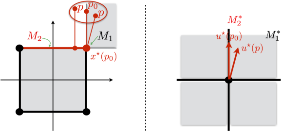
(a)

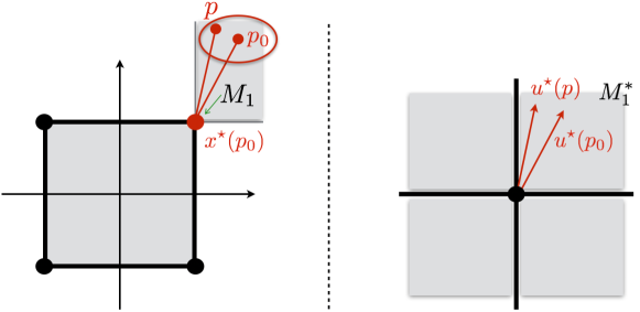
(b)

Fig. 3: Graphical illustration of Theorem 2 for a projection problem on the $\ell_{\infty}$ ball. (a) corresponds to a degenerate situation while (b) to a non-degenerate one.

Remark 7 (Single manifold identification).

In the special case where we have the non-degeneracy condition

$$u^{\star}(\mathring{p})=-\nabla F(x^{\star}(\mathring{p}),\mathring{p})\in\operatorname{ri}(\partial R(x^{\star}(\mathring{p}))),$$ (12)

our result simplifies and we recover the known exact identification result. To see this, we note that (12) also reads $u^{\star}(\mathring{p})\in\mathcal{J}_{R}(\{x^{\star}(\mathring{p})\})$, and thus $M^{*}_{u^{\star}(\mathring{p})}=\mathcal{J}_{R}(\{x^{\star}(\mathring{p})\})$. In this case, (11) becomes $M_{x^{\star}(p)}=M_{\mathring{x}}$ for all $p$ close to $\mathring{p}$. Such a result was also established in [35, 40] under condition (12), when $F(\cdot,\mathring{p})$ is also locally $C^{2}$ around $x^{\star}(\mathring{p})$ and $R$ is partly smooth at $x^{\star}(\mathring{p})$ relative to a $C^{2}$-smooth manifold $M_{x^{\star}(\mathring{p})}$. An example of this non-degenerate scenario is shown in Figure 3(b). Our result covers the more delicate degenerate situation where $u^{\star}(\mathring{p})$ might be on the relative boundary of the subdifferential, but requires the stronger mirror-stratifiability structure on the non-smooth part. However, the active set at $x^{\star}(p)$ is in general not unique for all $p$ close to $\mathring{p}$, hence the terminology enlarged activity.

Example 4.

The result of Theorem 2 is illustrated in Figure 3, for the projection problem on a $\ell_{\infty}$ ball, in both the degenerate and the non-degenerate situations. More precisely, we take $E(x,p)=\tfrac{1}{2}|\!|x-p|\!|^{2}+\iota_{\mathbb{B}_{\ell_{\infty}}}(x)$, so that $u^{\star}(p)=p-x^{\star}(p)$, where $x^{\star}(p)=\operatorname{P}_{\mathbb{B}_{\ell_{\infty}}}(p)$. Figure 3(a) illustrates the degenerate case where $u^{\star}(\mathring{p})$ belongs to the relative boundary of the normal cone of $\mathbb{B}_{\ell_{\infty}}$ at $x^{\star}(\mathring{p})$. Taking a perturbation $p$ around $\mathring{p}$ entails that $x^{\star}(p)$ belongs either to $M_{1}=M_{x^{\star}(\mathring{p})}$ or to the enlarged stratum $M_{2}=\mathcal{J}_{R^{*}}(M^{*}_{u^{\star}(\mathring{p})})=\mathcal{J}_{R^{*}}(M^{*}_{2})$. In the non-degenerate case of Figure 3(b) presented in Remark 7, the optimal solution $x^{\star}(p)$ is always on $M_{1}$ for small perturbations.

Remark 8 (Quadratic growth).

We can also establish the Lipschitz continuity of $x^{\star}(p)$ under the conditions of Theorem 2, under an additional second-order growth condition, just as in classical sensitivity analysis (see [7, Section 4.2.1]). Let us assume that there exists a neighbourhood $\mathcal{V}$ of $x^{\star}(\mathring{p})$ and $\kappa>0$ such that

$$E(x,\mathring{p})\geqslant E(x^{\star}(\mathring{p}),\mathring{p})+\kappa|\!|x-x^{\star}(\mathring{p})|\!|^{2}\qquad\forall x\in\mathcal{V}.$$ (13)

Since $x^{\star}_{k}\to x^{\star}(\mathring{p})$ for $p_{k}\to\mathring{p}$ (see the proof of Theorem 2), we have $x^{\star}_{k}\in\mathcal{V}$ for $k$ large enough. If, moreover, $\nabla F(x,\cdot)$ is Lipschitz-continuous in a neighbourhood of $\mathring{p}$ with Lipschitz constant $\nu$ independent of $x\in\mathcal{V}$, we get

$$\kappa|\!|x^{\star}_{k}-x^{\star}(\mathring{p})|\!|^{2} \leqslant E(x^{\star}_{k},\mathring{p})-E(x^{\star}(\mathring{p}),\mathring{p})$$

$$=\big{(}(E(x^{\star}(\mathring{p}),p_{k})-E(x^{\star}_{k},p_{k}))-(E(x^{\star}(\mathring{p}),\mathring{p})-E(x^{\star}_{k},\mathring{p}))\big{)}$$

$$\qquad-\big{(}E(x^{\star}(\mathring{p}),p_{k})-E(x^{\star}_{k},p_{k})\big{)}$$

($$x^{\star}_{k} E(\cdot,p_{k}) \leqslant(E(x^{\star}(\mathring{p}),p_{k})-E(x^{\star}_{k},p_{k}))-(E(x^{\star}(\mathring{p}),\mathring{p})-E(x^{\star}_{k},\mathring{p})$$ minimizes )

(By ($$\mathcal{P}(p) =(F(x^{\star}(\mathring{p}),p_{k})-F(x^{\star}_{k},p_{k}))-(F(x^{\star}(\mathring{p}),\mathring{p})-F(x^{\star}_{k},\mathring{p}))$$))

(Mean-Value Theorem) $$\leqslant\big{(}\sup_{x\in\mathcal{V}}|\!|\nabla F(x,p_{k})-\nabla F(x,\mathring{p})|\!|\big{)}|\!|x^{\star}_{k}-x^{\star}(\mathring{p})|\!|$$

$$\leqslant\nu|\!|p_{k}-\mathring{p}|\!||\!|x^{\star}_{k}-x^{\star}(\mathring{p})|\!|.$$

whence we conclude that

$$d(x^{\star}(\mathring{p}),\operatorname{Argmin}E(\cdot,p_{k}))\leqslant\nu/\kappa|\!|p_{k}-\mathring{p}|\!|.$$

4 Regularized Inverse Problems

A typical context where our framework of mirror-stratifiability is of usefulness is that of studying stability to noise of regularized linear inverse problems. We come back to the situation presented in introduction: studying stability issues to perturbed observations of the form $y=\mathring{y}+w$ amounts to analyzing sensitivity of the minimizers and the optimal value function in ($\mathcal{P}(\lambda,y)$) when the parameter $p=(\lambda,y)$ evolves around the reference point $\mathring{p}=(0,\mathring{y})$. Unlike the usual sensitivity analysis theory setting recalled in the previous section (e.g. [7]), here the objective $E$ may not even be continuous at $\mathring{p}$.

We provide hereafter some pointers to the relevant literature, then we develop our sensitivity results for mirror-stratifiable functions. These results involve primal and dual solutions to the noiseless problem

$$\underset{x\in\mathbb{R}^{N}}{\min}\;E(x,(0,y))\stackrel{{\scriptstyle\mbox{\tiny def.}}}{{=}}R(x)\quad\text{s.t.}\quad\Phi x=y, \mathcal{P}(0,y)$$ ()

4.1 Existing sensitivity results for regularized Inverse Problems

Lipschitz stability

Assume there exists a dual multiplier $\eta\in\mathbb{R}^{P}$ (sometimes referred to as a “dual certificate”) for the noiseless constrained problem ($\mathcal{P}(0,y)$) taken at $y=\mathring{y}$ such that $\Phi^{*}\eta\in\partial R(\mathring{x})$. The latter condition is equivalent to $\mathring{x}$ being a minimizer of ($\mathcal{P}(0,y)$). This condition goes by the name of the “source” or “range” condition in the inverse problems literature. It has been widely used to derive stability results in terms of $|\!|\Phi x^{\star}(\lambda,y)-\Phi\mathring{x}|\!|$ or $R(x^{\star}(\lambda,y))-R(\mathring{x})-\left\langle\Phi^{*}\eta,\,x^{\star}(\lambda,y)-\mathring{x}\right\rangle$; see [52] and references therein. To afford stability in terms of $|\!|x^{\star}(\lambda,y)-\mathring{x}|\!|$ directly, the range condition has to be strengthened to its non-degenerate version $\Phi^{*}\eta\in\operatorname{ri}(\partial R(\mathring{x}))$. It has been shown that this condition implies that the set-valued map $(\lambda,y)\mapsto x^{\star}(\lambda,y)$ is Lipschitz-continuous at $(0,\mathring{y})$; see [32] and [58].

Active set stability

In the case where $R$ is partly smooth, one can approach an even more complete sensitivity theory by studying stability of the partly smooth manifold of $R$ at $\mathring{x}$. In particular, it can be shown from that if an appropriate non-degeneracy assumption holds, see [59], then problems ($\mathcal{P}(0,y)$) and ($\mathcal{P}(\lambda,y)$) have unique minimizers (respectively $\mathring{x}$ and $x^{\star}(\lambda,y)$), and $x^{\star}(\lambda,y)$ lies on the partly smooth manifold of $R$ at $\mathring{x}$. Observe that compared to Lipschitz stability, active set stability is more demanding as the non-degeneracy condition has to hold for a specific dual multiplier, which is obviously more stringent. This type of results has appeared many times in the literature for special cases, e.g. for the $\ell_{1}$ norm [30, 61], the nuclear norm [1]. The work in [57, 59] has unified all these results.

Non-degeneracy in practice for deconvolution and compressed sensing

The above results require that some abstract non-degeneracy condition holds, which imposes strict limitations on practical situations. In particular, when $\Phi$ is a convolution operator and $\mathring{x}$ is sparse, [10] studies Lipschitz stability and [25] support stability. In this setting, the non-degeneracy condition holds whenever the non-zero entries are separated enough, which is not often verified. Another setting where this stability theory has been applied in when $\Phi$ is drawn from a random matrix ensemble, i.e. compressed sensing. For a variety of partly smooth regularizers (including the $\ell_{1}$, nuclear and $\ell_{1,2}$ norms), the non-degeneracy condition holds with high probability if, roughly speaking, the sample size $P$ is sufficiently larger than the “dimension” of the active set at $\mathring{x}$ (see e.g. [12, 22]). Again this is a clear limitation as illustrated in Section 1.2.

4.2 Primal and dual problems

Suppose we have observations of the form (1), and we want to recover $\mathring{x}$ (or a provably good approximation of it). As advocated in Section 1.1, a popular approach is to adopt a regularization framework which can be cast as the optimization problem ($\mathcal{P}(\lambda,y)$) (for $\lambda>0$) and ($\mathcal{P}(0,y)$) (when $\lambda=0$). In the sequel, we assume that

$$R^{\infty}(z)>0,\quad\forall z\in\ker(\Phi)\setminus\{0\},$$ (14)

where $R^{\infty}$ is the asymptotic (or recession) function of $R$, defined as

$$R^{\infty}(z)\stackrel{{\scriptstyle\mbox{\tiny def.}}}{{=}}\lim_{t\to+\infty}\frac{R(x+tz)-R(x)}{t},\quad\forall x\in\operatorname{dom}(R).$$

Condition (14) is a necessary and sufficient condition for the set of minimizers of ($\mathcal{P}(\lambda,y)$) and ($\mathcal{P}(0,y)$) to be non-empty and compact [56, Lemma 5.1]. It is satisfied for example when $R$ is coercive.

Remark 9 (Discontinuity of $F$).

Letting $p\stackrel{{\scriptstyle\mbox{\tiny def.}}}{{=}}(\lambda,y)\in\Pi\stackrel{{\scriptstyle\mbox{\tiny def.}}}{{=}}\mathbb{R}_{+}\times\mathbb{R}^{P}$, we see that ($\mathcal{P}(\lambda,y)$) and ($\mathcal{P}(0,y)$) are instances of ($\mathcal{P}(p)$), by setting

$$F(x,p)\stackrel{{\scriptstyle\mbox{\tiny def.}}}{{=}}\begin{cases}\frac{1}{2\lambda}|\!|y-\Phi x|\!|^{2}&\;\text{if}\;\lambda>0,\\ \iota_{\mathcal{H}_{y}}(x)&\;\text{if}\;\lambda=0,\end{cases}\quad\text{where}\quad\mathcal{H}_{y}\stackrel{{\scriptstyle\mbox{\tiny def.}}}{{=}}\left\{x\in\mathbb{R}^{N}\;:\;\Phi x=y\right\}.$$ (15)

The corresponding function $F$ considered does not obey the assumptions of Theorem 2. Indeed, the parameter set $\Pi$ is not open, with $\mathring{p}=(0,\mathring{y})$ that lives on the boundary of $\Pi$, and $F$ is only lsc at such $\mathring{p}$ (because of the affine constraint $\Phi x=y$). The main consequence will be that one can no longer allow $p$ to vary freely nearby $\mathring{p}$.

In order to study the sensitivity of solutions, we look at the Fenchel-Rockafellar dual problem, which reads (for all $\lambda\geqslant 0$)

$$\underset{q\in\mathbb{R}^{P}}{\max}\;\left\langle q,\,y\right\rangle-\frac{\lambda}{2}|\!|q|\!|^{2}-R^{*}(\Phi^{*}q). \mathcal{D}(\lambda,y)$$ ()

We denote $\mathfrak{D}(\lambda,y)$ the set of solutions of $(\mathcal{D}(\lambda,y))$. Note that for $\lambda>0$, thanks to strong concavity, there is a unique dual solution $q^{\star}(\lambda,y)$, i.e. $\mathfrak{D}(\lambda,y)=\{q^{\star}(\lambda,y)\}$. We also have from the primal-dual extremality relationship that for any primal solution $x^{\star}(\lambda,y)$ of ($\mathcal{P}(\lambda,y)$),

$$q^{\star}(p)=\frac{y-\Phi x^{\star}(p)}{\lambda}\quad\text{and}\quad\Phi^{*}q^{\star}(p)\in\partial R(x^{\star}(p)).$$ (16)

While $(\mathcal{D}(0,y))$ is the dual of $(\mathcal{P}(0,y))$, it is important to realize that it is not the limit of $(\mathcal{D}(\lambda,y))$ in the sense that its set of dual solutions is in general not a singleton. Lemma 3 hereafter singles out a specific dual optimal solution (sometimes called “minimum norm certificate”) defined by

$$\mathring{q}(0,y)=\underset{q\in\mathbb{R}^{P}}{\operatorname{argmin}}\left\{|\!|q|\!|\!\;:\;\Phi^{*}q\in\partial R(x^{\star}(0,y))\right\}=\underset{q\in\mathbb{R}^{P}}{\operatorname{argmin}}\left\{|\!|q|\!|\!\;:\;q\in\mathfrak{D}(0,y)\right\}.$$ (17)

The following two important lemmas ensure the convergence of the solutions to the primal and dual problems as $\lambda\rightarrow 0$ and as $|\!|y-\mathring{y}|\!|\to 0$.

Lemma 2 (Primal solution convergence).

Assume that $\mathring{x}$ is the unique solution to $(\mathcal{P}(0,\mathring{y}))$. For any sequence of parameters $p_{k}=(\lambda_{k},y_{k})$ with $\lambda_{k}>0$ such that

$$\left(\frac{|\!|y_{k}-\mathring{y}|\!|^{2}}{\lambda_{k}},\lambda_{k}\right)\longrightarrow(0,0),$$

and any solution $x^{\star}(p_{k})$ of $(\mathcal{P}(p_{k}))$, we have $x^{\star}(p_{k})\rightarrow\mathring{x}$.

Proof.

Denote $x^{\star}_{k}\stackrel{{\scriptstyle\mbox{\tiny def.}}}{{=}}x^{\star}(p_{k})$. Since $\left(x^{\star}_{k}\right)_{k\in\mathbb{N}}$ is a bounded sequence by (14), one can extract a converging subsequence, which for simplicity, we denote again $x^{\star}_{k}\rightarrow\bar{x}$. Optimality of $x^{\star}_{k}$ implies that

$$R(x^{\star}_{k})\leqslant\frac{1}{2\lambda_{k}}|\!|y_{k}-\Phi x^{\star}_{k}|\!|^{2}+R(x^{\star}_{k})\leqslant\frac{1}{2\lambda_{k}}|\!|y_{k}-\mathring{y}|\!|^{2}+R(\mathring{x}).$$ (18)

Passing to the limit and using the hypothesis that $\frac{1}{\lambda_{k}}|\!|y_{k}-\mathring{y}|\!|^{2}\rightarrow 0$, we get

$$\limsup_{k}R(x^{\star}_{k})\leqslant R(\mathring{x}).$$

On the other hand, lower semi-continuity of $R$ entails $\liminf_{k}R(x^{\star}_{k})\geqslant R(\bar{x}).$ Combining these two inequalities, we deduce that $R(\bar{x})\leqslant R(\mathring{x}).$ Since $R$ is proper and lsc, it is bounded from below on bounded sets [51, Corollary 1.10]. Let $\underline{r}=\inf_{k}R(x^{\star}_{k})$ which then satisfies $-\infty<\underline{r}<+\infty$. Substracting $\underline{r}$ from (18) and multiplying by $\lambda_{k}$, one obtains

$$\frac{1}{2}|\!|y_{k}-\Phi x^{\star}_{k}|\!|^{2}\leqslant\frac{1}{2}|\!|y_{k}-\Phi x^{\star}_{k}|\!|^{2}+\lambda_{k}(R(x^{\star}_{k})-\underline{r})\leqslant\frac{1}{2}|\!|y_{k}-\mathring{y}|\!|^{2}+\lambda_{k}(R(\mathring{x})-\underline{r}).$$ (19)

Consequently, passing to the limit in (19) shows that $|\!|\mathring{y}-\Phi\bar{x}|\!|=0$, i.e. $\bar{x}$ is a feasible point of $(\mathcal{P}(0,\mathring{y}))$. Altogether, this shows that $\bar{x}$ is a solution of $(\mathcal{P}(0,\mathring{y}))$, and by uniqueness of the minimizer, $\bar{x}=\mathring{x}$. ∎

Lemma 3 (Dual solution convergence).

For any sequence of parameters $p_{k}=(\lambda_{k},y_{k})$ such that

$$\left(\frac{|\!|y_{k}-\mathring{y}|\!|}{\lambda_{k}},\lambda_{k}\right)\longrightarrow(0,0),$$

we have $q^{\star}(p_{k})\rightarrow\mathring{q}(0,\mathring{y})$.

Proof.

By the triangle inequality, we have

$$|\!|q^{\star}(\lambda_{k},y_{k})-\mathring{q}(0,\mathring{y})|\!|\leqslant|\!|q^{\star}(\lambda_{k},y_{k})-q^{\star}(\lambda_{k},\mathring{y})|\!|+|\!|q^{\star}(\lambda_{k},\mathring{y})-\mathring{q}(0,\mathring{y})|\!|.$$

For the first term, we notice that $q^{\star}(\lambda,y)=\operatorname{prox}_{R^{*}\circ\Phi^{*}/\lambda}(y/\lambda)$ for $\lambda>0$. Thus, Lipschitz continuity of the proximal mapping entails that

$$|\!|q^{\star}(\lambda_{k},y_{k})-q^{\star}(\lambda_{k},\mathring{y})|\!|\leqslant\frac{|\!|y_{k}-\mathring{y}|\!|}{\lambda_{k}},$$

which in turn shows that $q^{\star}(\lambda_{k},y_{k})\to q^{\star}(\lambda_{k},\mathring{y})$. Let us now turn to the second term. Using the respective optimality of $q^{\star}_{k}=q^{\star}(\lambda_{k},\mathring{y})$ and $\mathring{q}\stackrel{{\scriptstyle\mbox{\tiny def.}}}{{=}}\mathring{q}(0,\mathring{y})\in\mathfrak{D}(0,\mathring{y})$, one obtains

$$-\left\langle q^{\star}_{k},\,\mathring{y}\right\rangle+\frac{\lambda_{k}}{2}|\!|q^{\star}_{k}|\!|^{2}+R^{*}(\Phi^{*}q^{\star}_{k}) \leqslant-\left\langle\mathring{q},\,\mathring{y}\right\rangle+\frac{\lambda_{k}}{2}|\!|\mathring{q}|\!|^{2}+R^{*}(\Phi^{*}\mathring{q})$$ (20)

$$\leqslant-\left\langle q^{\star}_{k},\,\mathring{y}\right\rangle+\frac{\lambda_{k}}{2}|\!|\mathring{q}|\!|^{2}+R^{*}(\Phi^{*}q^{\star}_{k}),$$

whence we get $|\!|q^{\star}_{k}|\!|\leqslant|\!|\mathring{q}|\!|$, which shows in particular that $\left(q^{\star}_{k}\right)_{k\in\mathbb{N}}$ is a bounded sequence. We can thus extract any converging subsequence, which for simplicity, we denote again $q^{\star}_{k}\rightarrow\bar{q}$. Passing to the limit in (20), using the fact that $R^{*}$ is lsc, one obtains

$$-\left\langle\bar{q},\,\mathring{y}\right\rangle+R^{*}(\Phi^{*}\bar{q})\leqslant-\left\langle\bar{q},\,\mathring{y}\right\rangle+\liminf_{k}R^{*}(\Phi^{*}q^{\star}_{k})\leqslant-\left\langle\mathring{q},\,\mathring{y}\right\rangle+R^{*}(\Phi^{*}\mathring{q}),$$

which shows that $\bar{q}\in\mathfrak{D}(0,\mathring{y})$. This together with the fact that $|\!|q^{\star}_{k}|\!|\leqslant|\!|\mathring{q}|\!|$ as we already saw, shows that $\bar{q}=\mathring{q}$ by uniqueness of $\mathring{q}$ in (17). ∎

4.3 Sensitivity

We are now in position to state the main result of this section, which tracks the strata of $x^{\star}(p)$ in the regime where the perturbation $|\!|w|\!|=|\!|y-\mathring{y}|\!|$ is sufficiently small.

Theorem 3.

Suppose that $\mathring{x}$ is the unique solution to $(\mathcal{P}(0,\mathring{y}))$. Assume furthermore that $R$ is mirror-stratifiable with respect to the primal-dual stratifications $(\mathcal{M},\mathcal{M}^{*})$. If there are constants $(C_{0},C_{1})$ depending only on $\mathring{x}$ such that for all $p$ in

$$\left\{p=(\lambda,y)\;:\;C_{0}|\!|y-\mathring{y}|\!|\leqslant\lambda\leqslant C_{1}\right\},$$ (21)

then there exists a minimizer $x^{\star}(p)$ of $E(\cdot,p)$ localized as follows

$$M_{\mathring{x}}\leqslant M_{x^{\star}(p)}\leqslant{\mathcal{J}_{R^{*}}}(M^{*}_{\mathring{u}})\quad\text{where}\quad\mathring{u}\stackrel{{\scriptstyle\mbox{\tiny def.}}}{{=}}\Phi^{*}\mathring{q}(0,\mathring{y}).$$ (22)

Proof.

Under (21) with for instance $C_{1}$ small enough, one can easly check that there exists $k$ large enough such that the regime required for $(y_{k},\lambda_{k})$ to apply Lemma 2 and 3 is attained. In turn, we have a converging primal-dual pair $(x^{\star}(p_{k}),\Phi^{*}q^{\star}(p_{k}))\rightarrow(\mathring{x},\mathring{u})$. One can then apply Theorem 1 to conclude. ∎

5 Activity Localization with Proximal Splitting Algorithms

Proximal splitting methods are algorithms designed to solve large-scale structured optimization and monotone inclusion problems, by evaluating various first-order quantities such as gradients, proximity operators, linear operators, all separately at various points in the course of an iteration. Though they can show slow convergence each iteration has a cheap cost. We refer to e.g. [3, 5, 17, 49] for a comprehensive treatment and review.

Capitalizing on our enlarged activity identification result for mirror-stratifiable functions, we now instantiate its consequences on finite activity localization of proximal splitting algorithms. While existing results on finite identification (of a single active set) strongly rely on partial smoothness around a non-degenerate cluster point [34, 42, 43, 41], we examine here intricate situations where neither of these assumptions holds.

5.1 Forward-Backward algorithm

The Forward–Backward (FB) splitting method [44] is probably the most well-known proximal splitting algorithm. In our context, it can be used to solve optimization problems with the additive “smooth + non-smooth” structure of the form

$$\min_{x\in\mathbb{R}^{N}}f(x)+R(x),$$ (23)

where $f\in C^{1}(\mathbb{R}^{N})$ is convex with $L$-Lipschitz gradient, and $R$ is a proper lsc and convex function. We assume that $\operatorname{Argmin}(f+R)\neq\emptyset$. The FB iteration in relaxed form reads [16]

$$x_{k+1}=(1-\tau_{k})x_{k}+\tau_{k}\operatorname{prox}_{\gamma_{k}R}(x_{k}-\gamma_{k}\nabla f(x_{k})),$$ (24)

with $\gamma_{k}\in]0,2/L[$ and $\tau_{k}\in]0,1]$, where $\operatorname{prox}_{\gamma R}$, $\gamma>0$, is the proximal mapping of $R$,

$$\operatorname{prox}_{\gamma R}(x)\stackrel{{\scriptstyle\mbox{\tiny def.}}}{{=}}\underset{z\in\mathbb{R}^{N}}{\operatorname{argmin}}\frac{1}{2}|\!|z-x|\!|^{2}+\gamma R(z).$$ (25)

Different variants of FB method were studied, and a popular trend is the inertial schemes which aim at speeding up the convergence (see [48, 4], and the sequence-convergence version as proved recently in [14]).

Under the non-degeneracy assumption $-\nabla f(x^{\star})\in\operatorname{ri}(\partial R(x^{\star}))$, it was shown in [42] that FB and its inertial variants correctly identify the active manifold in finitely many iterations, and then enter a local linear convergence regime. These results encompass many special cases such as those studied in [33, 8, 54]. Beyond this non-degenerate case, we establish now the general localization of active strata.

Theorem 4.

Consider the FB iteration (24) to solve (23) with $0<\inf_{k}\gamma_{k}\leqslant\sup_{k}\gamma_{k}<2/L$ and $\inf_{k}\tau_{k}>0$. Then $x_{k}$ converges to $x^{\star}\in\operatorname{Argmin}(f+R)$. Assume that $R$ is also mirror-stratifiable with respect to $(\mathcal{M},\mathcal{M}^{*})$, then for $k$ large enough,

$$M_{x^{\star}}\leqslant M_{x_{k}}\leqslant\mathcal{J}_{R^{*}}(M^{*}_{u^{\star}})\quad\text{where}\quad u^{\star}\stackrel{{\scriptstyle\mbox{\tiny def.}}}{{=}}-\nabla f(x^{\star}).$$

Proof.

Convergence of the sequence $\left(x_{k}\right)_{k\in\mathbb{N}}$ to $x^{\star}$ is obtained from [16, Corollary 6.5]. Moreover, since the proximal mapping is the resolvent of the subdifferential, (24) is equivalent to the monotone inclusion

$$u_{k+1}\stackrel{{\scriptstyle\mbox{\tiny def.}}}{{=}}\frac{x_{k}-v_{k+1}}{\gamma_{k}}-\nabla f(x_{k})\in\partial R(v_{k+1}),$$

where $v_{k+1}\stackrel{{\scriptstyle\mbox{\tiny def.}}}{{=}}\frac{x_{k+1}-x_{k}}{\tau_{k}}+x_{k}$. In turn, with the conditions $\inf_{k}\tau_{k}>0$ and $\inf_{k}\gamma_{k}>0$, and continuity of $\nabla f$, we have $v_{k}\to x^{\star}$ and thus $u_{k}\to-\nabla f(x^{\star})\in\partial R(x^{\star})$. It then remains to apply Theorem 1 to $(v_{k},u_{k})$ and $R$ to conclude. ∎

It can be easily shown that Theorem 4 holds for several extensions of the iterate-convergent version of FISTA [14]. We omit the details here for the sake of brevity.

We rather take a closer look to the case when the FB scheme (24) to solve ($\mathcal{P}(\lambda,y)$) (see also (15)) for $\lambda>0$. Putting together Theorem 3 and 4, we obtain the following localization result depending only on the data to estimate $\mathring{x}$ assuming that the noise level $|\!|y-\mathring{y}|\!|$ is small enough.

Proposition 4.

Under the assumptions of Theorem 3, consider the FB iteration (24) to solve ($\mathcal{P}(\lambda,y)$) with $0<\inf_{k}\gamma_{k}\leqslant\sup_{k}\gamma_{k}<2\lambda/|\!|\Phi|\!|^{2}$ and $\inf_{k}\tau_{k}>0$. Then, for $k$ large enough, the iterates $x_{k}$ satisfy

$$M_{\mathring{x}}\leqslant M_{x_{k}}\leqslant\mathcal{J}_{R^{*}}(M_{\mathring{u}}^{*})\quad\text{where}\quad\mathring{u}\stackrel{{\scriptstyle\mbox{\tiny def.}}}{{=}}\Phi^{*}q(0,\mathring{y}),$$

with $q(0,\mathring{y})$ from (17).

Proof.

To lighten notation, denote $p=(\lambda,y)$. As in Theorem 4, we have $x_{k}\to x^{\star}(p)$ a minimizer of ($\mathcal{P}(\lambda,y)$). Thus we get

$$M_{\mathring{x}}\leqslant M_{x^{\star}(p)}\leqslant M_{x_{k}},$$

where the first inequality comes from Theorem 3 and the second one from Theorem 4. This gives the first inequality in the localization result.

Moreover, in the special case at hand $\partial R(x^{\star}(p))\ni-\nabla f(x^{\star}(p))=\Phi^{*}q^{\star}(p)\to\mathring{u}$ as $p\to(0,\mathring{y})$, where we invoked (16). It then follows from (9) and the fact that $\mathcal{J}_{R^{*}}$ is decreasing for the relation $\leqslant$, that

$$M^{*}_{\mathring{u}}\leqslant M^{*}_{-\nabla f(x^{\star}(p))}\iff\mathcal{J}_{R^{*}}(M^{*}_{-\nabla f(x^{\star}(p))})\leqslant\mathcal{J}_{R^{*}}(M^{*}_{\mathring{u}}).$$

Using once again Theorem 4, we get

$$M_{x_{k}}\leqslant\mathcal{J}_{R^{*}}(M^{*}_{-\nabla f(x^{\star}(p))})\leqslant\mathcal{J}_{R^{*}}(M^{*}_{\mathring{u}}),$$

which yields the second desired inequality. ∎

Though the iterates $x_{k}$ of FB do not converge to $\mathring{x}$, this proposition tells us that the iterates identify an enlarged stratum associated to $\mathring{x}$. This is an appealing feature from a practical perspective, since one can often make some prior assumption on the sought after vector $\mathring{x}$, such as for instance sparsity or low-rank properties, as we have illustrated in the numerical experiments of Section 6.

5.2 Douglas-Rachford Splitting Algorithm

The Douglas-Rachford (DR) method [44] is another popular splitting method designed to minimize convex objectives having the additive “non-smooth + non-smooth” structure of the form

$$\min_{x\in\mathbb{R}^{N}}f(x)+g(x).$$ (26)

with $f$ and $g$ be proper lsc and convex functions such that $\operatorname{ri}(\operatorname{dom}(f))\cap\operatorname{ri}(\operatorname{dom}(g))\neq\emptyset$ and $\operatorname{Argmin}(f+g)\neq\emptyset$. The DR scheme reads

$$\begin{cases}v_{k+1}&=\operatorname{prox}_{\gamma f}\left(2x_{k}-z_{k}\right),\\ z_{k+1}&=z_{k}+{\tau_{k}}\left(v_{k+1}-x_{k}\right),\\ x_{k+1}&=\operatorname{prox}_{\gamma g}(z_{k+1}),\end{cases}$$ (27)

where $\gamma>0$, $\tau_{k}\in]0,2[$ is a relaxation parameter. By definition, the DR method is not symmetric with respect to the order of the functions $f$ and/or $g$. Nevertheless, all of our statements throughout hold true, with obvious adaptations, when the order of $f$ and $g$ is reversed in (27).

It has been shown in [43] that under appropriate non-degeneracy assumptions, the DR identifies the active manifolds in finite time, and then shows a local linear regime. These results unify all those that were established in the literature for special problems, see e.g. [20] for linearly constrained $\ell_{1}$-minimization, [6] for quadratic or linear programs, [2] for feasibility with two subspaces. Under mirror-stratifiability of $f$ or $g$, we get the following enlarged activity identification result.

Theorem 5.

Consider the DR iteration (27) to solve (26) with $\tau_{k}\in]0,2[$ such that $\sum_{k\in\mathbb{N}}\tau_{k}\left(2-\tau_{k}\right)=+\infty$. Then $z_{k}$ converges to a fixed point $z^{\star}$ with $x^{\star}=\operatorname{prox}_{\gamma g}(z^{\star})\in\operatorname{Argmin}(f+g)$, and $x_{k}$ and $v_{k}$ both converge to $x^{\star}$. Introducing $u^{\star}=\frac{z^{\star}-x^{\star}}{\gamma}$, we have furthermore:

1. If $g$ is mirror-stratifiable with respect to the primal-dual stratifications $(M^{g},M^{g^{*}})$, then for $k$ large enough

   $$M^{g}_{x^{\star}}\leqslant M^{g}_{x_{k}}\leqslant\mathcal{J}_{g^{*}}(M^{g^{*}}_{u^{\star}}).$$

2. If $f$ is mirror-stratifiable with respect to the primal-dual stratifications $(M^{f},M^{f^{*}})$, then for $k$ large enough

   $$M^{f}_{x^{\star}}\leqslant M^{f}_{v_{k}}\leqslant\mathcal{J}_{f^{*}}(M^{f^{*}}_{-u^{\star}}).$$

Proof.

Under the prescribed choice of $\tau_{k}$, convergence of $z_{k}$ is ensured by virtue of [16, Corollary 5.2]. By non-expansiveness of the proximal mapping, and as we are in finite dimension, we also obtain convergence of $x_{k}$ and $v_{k}$ to $x^{\star}$. To prove (i), note that the update of $x_{k}$ in (27) is equivalent to the monotone inclusion

$$u_{k}\stackrel{{\scriptstyle\mbox{\tiny def.}}}{{=}}\frac{z_{k}-x_{k}}{\gamma}\in\partial g(x_{k}).$$ (28)

Since $(x_{k},u_{k})\to(x^{\star},u^{\star})$, we conclude about (i) by invoking Theorem 1. Similarly, we note that the update of $v_{k}$ in (27) is equivalent to

$$w_{k}\stackrel{{\scriptstyle\mbox{\tiny def.}}}{{=}}\frac{2x_{k}-z_{k}-v_{k+1}}{\gamma}\in\partial f(v_{k+1}).$$ (29)

Using that $(v_{k},w_{k})\to(x^{\star},-u^{\star})$ and applying Theorem 1 we get (ii). ∎

In the same vein as for FB in the previous section, we now turn to applying the DR scheme (27) to solve ($\mathcal{P}(\lambda,y)$) by setting in (26) $f(x)=\frac{1}{2\lambda}|\!|y-\Phi x|\!|^{2}$ and $g(x)=R(x)$. Putting Theorem 3 and 5-(i) together, we obtain the following analogue to Proposition 4.

Proposition 5.

Under the assumptions of Theorem 3, consider the DR iteration (27) to solve ($\mathcal{P}(\lambda,y)$) with $\gamma>0$ and $\tau_{k}\in]0,2[$ such that $\sum_{k\in\mathbb{N}}\tau_{k}\left(2-\tau_{k}\right)=+\infty$. Then, for $k$ large enough, the DR iterates satisfy

$$M_{\mathring{x}}\leqslant M_{x_{k}}\leqslant\mathcal{J}_{R^{*}}(M_{\mathring{u}}^{*})\quad\text{where}\quad\mathring{u}\stackrel{{\scriptstyle\mbox{\tiny def.}}}{{=}}\Phi^{*}q(0,\mathring{y}).$$

Proof.

The proof follows the same reasoning as that of Proposition 4 by additionally observing (recall the notation in the proof of Theorem 5) that from (28)-(29), we have $u^{\star}(p)=-\nabla f(x^{\star}(p))=\Phi^{*}q^{\star}(p)\in\partial R(x^{\star}(p))$. ∎

6 Numerical Illustrations

In this section, we numerically illustrate our theoretical results on sensitivity and enlarged activity identification in the context of regularized inverse problems. We adopt the same two “compressed sensing” scenarios described in Section 1.2. The dimension $\dim(M_{\mathring{x}})=R_{0}(\mathring{x})$ of the strata associated to $\mathring{x}$ is measured as $R_{0}=|\!|\cdot|\!|_{0}$ (resp. $R_{0}=\mathop{\operator@font rank}\nolimits$) for the $\ell_{1}$ (resp. nuclear) norm regularization.

Strata sensitivity

We first illustrate the relevance of the strata sensitivity result in Theorem 3 by studying the dimension of the largest possible active stratum ${\mathcal{J}_{R^{*}}}(M^{*}_{\mathring{u}})$ (in fact its closure). The dual $\mathring{u}=\Phi^{*}\mathring{q}(0,\mathring{y})$ is computed from $\mathring{x}$ by solving the convex optimization problem (17) (using CVX to get a high precision). Thus we know the maximum complexity index excess predicted by Theorem 3, i.e.

$$\delta^{\star}(\mathring{x})\stackrel{{\scriptstyle\mbox{\tiny def.}}}{{=}}\dim({\mathcal{J}_{R^{*}}}(M^{*}_{\mathring{u}}))-\dim(M_{\mathring{x}}).$$

For each given $\delta$ and $R_{0}(\mathring{x})$, and among the 1000 randomly generated replications of $(\mathring{x},\Phi)$, we compute the proportion $\rho(R_{0}(\mathring{x}),\delta)$ of $\mathring{x}$ such that it is the unique solution of $(\mathcal{P}(0,\mathring{y}))$ and $\delta^{\star}(\mathring{x})\leqslant\delta$. The proportions $\rho(R_{0}(\mathring{x}),\delta)$ are displayed in Figure 4 as a function of the input complexity index $R_{0}(\mathring{x})=\dim(M_{\mathring{x}})$. The colors from blue to red correspond to increasing $\delta$.

The proportion $\rho(R_{0}(\mathring{x}),\delta)$ is an increasing function of $\delta$ and a decreasing function of $R_{0}(\mathring{x})$. Indeed, as anticipated from standard compressed sensing results [58], active strata $M_{\mathring{x}}$ of vectors $\mathring{x}$ whose dimension is small enough compared to the number of measurements $P$ can be provably and stably recovered with overwhelming probability (on the sampling of $(\mathring{x},\Phi,w)$). As $R_{0}(\mathring{x})$ increases, the number of measurements $P$ becomes insufficient to ensure non-degeneracy with high probability, hence preventing stable recovery of $M_{\mathring{x}}$. However, Theorem 3 predicts that the active stratum of $x^{\star}(\lambda,y)$ for $y$ nearby $\mathring{y}$ is localized between $M_{\mathring{x}}$ and ${\mathcal{J}_{R^{*}}}(M^{*}_{\mathring{u}})$.

The blue curve in each plot of Figure 4 corresponds to $\delta=0$, which is the proportion $\rho(R_{0}(\mathring{x}),0)$ of vectors $\mathring{x}$ whose active stratum $M_{\mathring{x}}$ can be recovered stably under small noise perturbation by solving ($\mathcal{P}(\lambda,y)$) for $\lambda$ chosen according to (21). This proportion shows a phase transition phenomenon between stable recovery and unstable recovery. The location of the phase transition for $\delta=0$ can be predicted accurately; see for instance [59].

The red curves in Figure 4 correspond to the extreme case where $\delta$ takes its largest achievable value, i.e. where we can guarantee recovery of the largest stratum ${\mathcal{J}_{R^{*}}}(M^{*}_{\mathring{u}})$ with high probability. The phase transition occurs for higher dimension $R_{0}(\mathring{x})$. The intermediate curves, i.e. from blue to red, correspond to the recovered strata that are localized between $M_{\mathring{x}}$ and ${\mathcal{J}_{R^{*}}}(M^{*}_{\mathring{u}})$ (i.e. increasing $\delta$). The phase transition progressively increases with $\delta$. These curves illustrate and quantify the typical tradeoff observed in practice: one can allow for more complex input vectors $\mathring{x}$ (i.e. those with larger $R_{0}(\mathring{x})$) at the expense of recovering active strata larger than $M_{\mathring{x}}$.

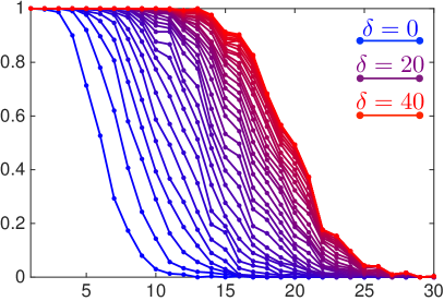
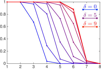
$R=|\!|\cdot|\!|_{1}$	$R=|\!|\cdot|\!|_{*}$

Fig. 4: Proportion of $\mathring{x}$ such that $\delta^{\star}(\mathring{x})\leqslant\delta$ as a function of $R_{0}(\mathring{x})$ (increasing value of $\delta$ from $0$ to its maximal value is depicted by a color evolving from blue to red).

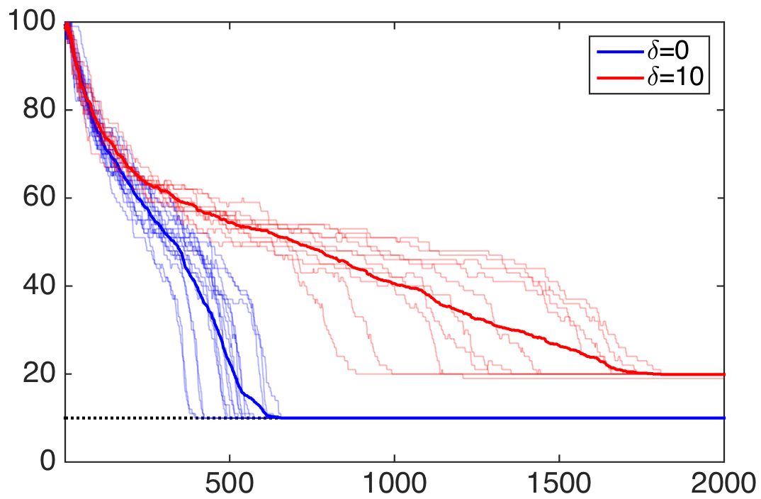
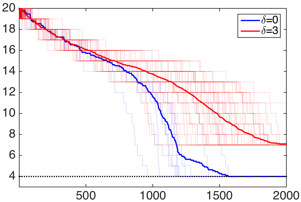
$R=|\!|\cdot|\!|_{1}$	$R=|\!|\cdot|\!|_{*}$

Fig. 5: Plots of $R_{0}(x_{k})$ for the 2000 first iterates generated by the Forward-Backward algorithm. Plots in blue correspond to the cases when $\delta^{\star}(\mathring{x})=0$, and the red ones for $\delta^{\star}(\mathring{x})=\delta$.

Forward-Backward finite activity localization

We now numerically illustrate the finite enlarged activity identification of the FB splitting scheme as predicted by Theorem 4 and Proposition 4. We remain under the same compressed sensing setting as before. The randomly generated replications of $\mathring{x}$ are such that $R_{0}(\mathring{x})=10$ for $R=|\!|\cdot|\!|_{1}$ and to $4$ for $R=|\!|\cdot|\!|_{*}$.

The evolution of the complexity index $R_{0}(x_{k})$ of the FB iterate $x_{k}$ is shown in Figure 5. The blue lines correspond to several trajectories (the bold one is the average trajectory), each for a randomly generated instance of $\mathring{x}$ such that $\delta^{\star}(\mathring{x})=0$, i.e. those vectors whose active strata $M_{\mathring{x}}$ can be exactly recovered under small perturbations. Thus, the iterates identify $M_{\mathring{x}}$ in finite time. The red lines (the bold one is the average trajectory) are those for which $\delta^{\star}(\mathring{x})=\delta>0$. As anticipated by our theoretical results, the iterates identify a stratum strictly larger that $M_{\mathring{x}}$.

Appendix A Proofs of the results in Section 2

Proof of Proposition 1

Let us first prove the first equivalence. Observe that Definition 2 can be read as follows: $M$ is active at $x$ if and only if $d(x,\operatorname{cl}(M))=0$. Since there is a finite number of strata in the stratification, let us consider $\delta$ the minimum of the nonzero distances $d(x,\operatorname{cl}(M^{\prime}))$ for $M^{\prime}$ not active. For all $x^{\prime}$ in the open ball of radius $\delta$ and of center $x$, we have

$$d(x,\operatorname{cl}(M_{x^{\prime}}))\leqslant|\!|x-x^{\prime}|\!|<\delta\qquad\iff\qquad d(x,\operatorname{cl}(M_{x^{\prime}}))=0.$$

This shows that the set of these strata $M_{x^{\prime}}$ indeed coincides the set of active strata, whence we get the first equivalence.

Let us turn to the second equivalence. Let $M$ be an active strata at $x$, that is, $x\in\operatorname{cl}(M)$. Since $x\in M_{x}$, the intersection $\operatorname{cl}(M)\cap M_{x}$ contains $x$ and thus is nonempty. We deduce from (3) that $M\geqslant M_{x}$. Conversely, if $M\geqslant M_{x}$, then $x\in M_{x}\subset\operatorname{cl}(M)$ and therefore $M$ is active at $x$.

Proof of Proposition 2

From classical convex analysis calculus rules, we get for all $x\in\operatorname{dom}R$

$$\partial R(x)=\operatorname{conv}\left\{a_{i}\;:\;i\in I^{\max}(x)\right\}+\operatorname{cone}\left\{a_{i}\;:\;i\in I^{\operatorname{feas}}(x)\right\}.$$

By definition of $M_{I}$, the relative interior of $\partial R(x)$ is constant over a stratum: for all $x\in M_{I}$ (with $M_{I}\neq\emptyset$)

$$\operatorname{ri}(\partial R(x)) = \operatorname{ri}\big{(}\operatorname{conv}\left\{a_{i}\;:\;i\in I^{\max}(x)\right\}+\operatorname{cone}\left\{a_{i}\;:\;i\in I^{\operatorname{feas}}(x)\right\}\big{)}$$

$$= \operatorname{ri}(\operatorname{conv}\left\{a_{i}\;:\;i\in I^{\max}(x)\right\})+\operatorname{ri}(\operatorname{cone}\left\{a_{i}\;:\;i\in I^{\operatorname{feas}}(x)\right\})$$

$$= \operatorname{ri}(\operatorname{conv}\left\{a_{i}\;:\;i\in I^{\max}\right\})+\operatorname{ri}(\operatorname{cone}\left\{a_{i}\;:\;i\in I^{\operatorname{feas}}\right\}).$$

This yields $\mathcal{J}_{R}(M_{I})=M^{*}_{I}$. Conversely we have $\partial R^{*}(u)=\left\{x\;:\;u\in\partial R(x)\right\}$, which entails for all $u\in M_{I}^{*}$

$$\partial R^{*}(u)=\left\{x\;:\;I^{\max}(x)\cap I^{\operatorname{feas}}(x)\supset I\right\},$$

and therefore $\operatorname{ri}(\partial R^{*}(u))=M_{I}$. This gives $\mathcal{J}_{R^{*}}(M^{*}_{I})=M_{I}$, which proves item (i) of Definition 4.

To show (ii) of Definition 4, we make the following observation:

$$M_{I}\leqslant M_{I^{\prime}} \Longleftrightarrow\text{any $x\in M_{I}$ lies in $\operatorname{cl}(M_{I^{\prime}})$}$$

$$\Longleftrightarrow I^{\max}=I^{\max}(x)\supset{(I^{\prime})}^{\max}\quad\text{and}\quad I^{\operatorname{feas}}=I^{\operatorname{feas}}(x)\supset{(I^{\prime})}^{\operatorname{feas}}$$

$$\Longleftrightarrow I\supset I^{\prime}.$$

On the other hand we have

$$\operatorname{cl}(\mathcal{J}_{R}(M_{I})) \supset\operatorname{cl}(\operatorname{ri}(\operatorname{conv}\left\{a_{i}\;:\;i\in I^{\max}\right\}))+\operatorname{cl}(\operatorname{ri}\operatorname{cone}\left\{a_{i}\;:\;i\in I^{\operatorname{feas}}\right\}))$$

$$=\operatorname{conv}\left\{a_{i}\;:\;i\in I^{\max}\right\}+\operatorname{cone}\left\{a_{i}\;:\;i\in I^{\operatorname{feas}}\right\}.$$

Note that the first $\supset$ is in fact $=$ because $\operatorname{conv}\left\{a_{i}\;:\;i\in I^{\max}\right\}$ is compact. Using unique decomposition of a polyhedron, we can write,

$$\mathcal{J}_{R}(M_{I})\geqslant\mathcal{J}_{R}(M_{I^{\prime}})\Longleftrightarrow\operatorname{cl}(\mathcal{J}_{R}(M_{I}))\supset\mathcal{J}_{R}(M_{I^{\prime}})\Longleftrightarrow I\supset I^{\prime},$$

which ends the proof.

Proof of Proposition 3

The proof builds upon a key result stated in [19]. Theorem 4.6(i) in [19] asserts that the collection $\left\{\sigma^{-1}(M^{\operatorname{sym}})\;:\;M\in\mathcal{M}\right\}$ forms a smooth stratification of $\operatorname{dom}(R)$ with the desired properties. The fact that spectral functions are mirror-stratifiable follows from the polyhedral case with the help of Theorem 4.6(iv) in [19], which states that

$$\mathcal{J}_{R}(\sigma^{-1}(M^{\operatorname{sym}}))=\sigma^{-1}\big{(}\mathcal{J}_{R^{\operatorname{sym}}}(M^{\operatorname{sym}})\big{)}$$

together with continuity of the singular value mapping $\sigma$.

References

- [1] F. Bach. Consistency of trace norm minimization. The Journal of Machine Learning Research, 9(Jun):1019–1048, 2008.
- [2] H. Bauschke, J.Y.B. Cruz, T.A. Nghia, H.M. Phan, and X. Wang. The rate of linear convergence of the douglas-rachford algorithm for subspaces is the cosine of the friedrichs angle. J. of Approx. Theo., 185(63–79), 2014.
- [3] H. H. Bauschke and P. L. Combettes. Convex analysis and monotone operator theory in Hilbert spaces. Springer, 2011.
- [4] A. Beck and M. Teboulle. A fast iterative shrinkage-thresholding algorithm for linear inverse problems. SIAM Journal on Imaging Sciences, 2(1):183–202, 2009.
- [5] A. Beck and M. Teboulle. Gradient-based algorithms with applications to signal recovery. Convex Optimization in Signal Processing and Communications, 2009.
- [6] D. Boley. Local linear convergence of the alternating direction method of multipliers on quadratic or linear programs. SIAM J. Optim., 23(4):2183–2207, 2013.
- [7] J. F. Bonnans and A. Shapiro. Perturbation analysis of optimization problems. Springer Series in Operations Research and Financial Engineering. Springer Verlag, 2000.
- [8] K. Bredies and D. A. Lorenz. Linear convergence of iterative soft-thresholding. Journal of Fourier Analysis and Applications, 14(5-6):813–837, 2008.
- [9] P. Bühlmann and S. Van De Geer. Statistics for high-dimensional data: methods, theory and applications. Springer, 2011.
- [10] E. J. Candès and C. Fernandez-Granda. Towards a mathematical theory of super-resolution. Communications on Pure and Applied Mathematics, 67(6):906–956, 2013.
- [11] E. J. Candès and B. Recht. Exact matrix completion via convex optimization. Foundations of Computational mathematics, 9(6):717–772, 2009.
- [12] E. J. Candès and T. Tao. Decoding by linear programming. Information Theory, IEEE Transactions on, 51(12):4203–4215, 2005.
- [13] E. J. Candès and T. Tao. The power of convex relaxation: Near-optimal matrix completion. Information Theory, IEEE Transactions on, 56(5):2053–2080, 2010.
- [14] A. Chambolle and C. Dossal. On the convergence of the iterates of the “fast iterative shrinkage/thresholding algorithm”. Journal of Optimization Theory and Applications, 166(3):968–982, 2015.
- [15] S. S. Chen, D. L. Donoho, and M. A. Saunders. Atomic decomposition by basis pursuit. SIAM journal on scientific computing, 20(1):33–61, 1999.
- [16] P. L. Combettes. Solving monotone inclusions via compositions of nonexpansive averaged operators. Optimization, 53(5-6):475–504, 2004.
- [17] P. L. Combettes and J.-C. Pesquet. Proximal splitting methods in signal processing. In H. H. Bauschke, Burachik R. S., P. L. Combettes, Elser. V., D. R. Luke, and H. Wolkowicz, editors, Fixed-Point Algorithms for Inverse Problems in Science and Engineering, pages 185–212. Springer, 2011.
- [18] M. Coste. An introduction to o-minimal geometry. Technical report, Institut de Recherche Mathematiques de Rennes, November 1999.
- [19] A. Daniilidis, D. Drusvyatskiy, and A. S. Lewis. Orthogonal invariance and identifiability. SIAM Journal on Matrix Analysis and Applications, 35(2):580–598, 2014.
- [20] L. Demanet and X. Zhang. Eventual linear convergence of the douglas-rachford iteration for basis pursuit. Mathematics of Computation, 2013. to appear.
- [21] A. L. Dontchev. Perturbations, approximations, and sensitivity analysis of optimal control systems, volume 52. Springer-Verlag, Berlin, 1983.
- [22] C. Dossal, M.-L. Chabanol, G. Peyré, and J. M. Fadili. Sharp support recovery from noisy random measurements by -minimization. Applied and Computational Harmonic Analysis, 33(1):24–43, 2012.
- [23] D. Drusvyatskiy, A. D. Ioffe, and A. S. Lewis. Generic minimizing behavior in semialgebraic optimization. SIAM J. Optim., 26(1):513–534, 2016.
- [24] D. Drusvyatskiy and A.S. Lewis. Optimality, identifiability, and sensitivity. Mathematical Programming, to appear in, pages 1–32, 2013.
- [25] V. Duval and G. Peyré. Exact support recovery for sparse spikes deconvolution. Foundations of Computational Mathematics, 15(5):1315–1355, 2015.
- [26] V. Duval and G. Peyré. Sparse spikes deconvolution on thin grids. Preprint 01135200, HAL, 2015.
- [27] C. Ekanadham, D. Tranchina, and E. P. Simoncelli. A unified framework and method for automatic neural spike identification. Journal of Neuroscience Methods, 222:47 – 55, 2014.
- [28] M. Fazel. Matrix Rank Minimization with Applications. PhD thesis, Stanford University, 2002.
- [29] A. V. Fiacco and G. P. McCormick. Nonlinear Programming: Sequential Unconstrained Minimization Techniques. Wiley, New York, 1968. reprinted, SIAM, Philadelphia, 1990.
- [30] J.-J. Fuchs. On sparse representations in arbitrary redundant bases. Information Theory, IEEE Transactions on, 50(6):1341–1344, 2004.
- [31] Michael Grant and Stephen Boyd. CVX: Matlab software for disciplined convex programming, version 2.1. http://cvxr.com/cvx, March 2014.
- [32] M. Grasmair, O. Scherzer, and M. Haltmeier. Necessary and sufficient conditions for linear convergence of l1-regularization. Communications on Pure and Applied Mathematics, 64(2):161–182, 2011.
- [33] E. Hale, W. Yin, and Y. Zhang. Fixed-point continuation for -minimization: methodology and convergence. SIAM J. Optim., 19(3):1107–1130, 2008.
- [34] W. L. Hare. Identifying active manifolds in regularization problems. In H. H. Bauschke, R. S., Burachik, P. L. Combettes, V. Elser, D. R. Luke, and H. Wolkowicz, editors, Fixed-Point Algorithms for Inverse Problems in Science and Engineering, volume 49 of Springer Optimization and Its Applications, chapter 13. Springer, 2011.
- [35] W. L. Hare and A. S. Lewis. Identifying active constraints via partial smoothness and prox-regularity. J. Convex Anal., 11(2):251–266, 2004.
- [36] J.-B. Hiriart-Urruty and H. Y. Le. Convexifying the set of matrices of bounded rank: applications to the quasiconvexification and convexification of the rank function. Optimization Letters, 6(5):841–849, 2012.
- [37] Hai Yen Le. Confexifying the Counting Function on Rp for Convexifying the Rank Function on Mm,n(R). Journal of Convex Analysis, 19(2):519–524, 2012.
- [38] C. Lemaréchal, F. Oustry, and C. Sagastizábal. The -lagrangian of a convex function. Trans. Amer. Math. Soc., 352(2):711–729, 2000.
- [39] A. S. Lewis. Active sets, nonsmoothness, and sensitivity. SIAM J. Optim., 13(3):702–725, 2002.
- [40] A. S. Lewis and S. Zhang. Partial smoothness, tilt stability, and generalized hessians. SIAM J. Optim., 23(1):74–94, 2013.
- [41] J. Liang. Convergence Rates of First-Order Operator Splitting Methods. Theses, Normandie Université, October 2016.
- [42] J. Liang, J. Fadili, and G. Peyré. Activity identification and local linear convergence of forward–backward-type methods. SIAM J. Optim., 27(1):408–437, 2017.
- [43] J. Liang, J. Fadili, and G. Peyré. Local convergence properties of douglas–rachford and alternating direction method of multipliers. Journal of Optimization Theory and Applications, 172(3):874–913, 2017.
- [44] P. L. Lions and B. Mercier. Splitting algorithms for the sum of two nonlinear operators. SIAM Journal on Numerical Analysis, 16(6):964–979, 1979.
- [45] S. G. Mallat. A wavelet tour of signal processing. Elsevier, third edition, 2009.
- [46] S. A. Miller and J. Malick. Newton methods for nonsmooth convex minimization: connections among-Lagrangian, Riemannian Newton and SQP methods. Mathematical programming, 104(2-3):609–633, 2005.
- [47] B. S. Mordukhovich. Sensitivity analysis in nonsmooth optimization. In D. A. Field and V. Komkov, editors, Theoretical Aspects of Industrial Design, volume 58, pages 32–46. SIAM Volumes in Applied Mathematics, 1992.
- [48] Y. Nesterov. A method for solving the convex programming problem with convergence rate . Dokl. Akad. Nauk SSSR, 269(3):543–547, 1983.
- [49] N. Parikh and S. P. Boyd. Proximal algorithms. Foundations and Trends in Optimization, 1(3):123–231, 2013.
- [50] R. T. Rockafellar. Convex analysis. Number 28 in Princeton Mathematical Series. Princeton university press, 1970.
- [51] R. T. Rockafellar and R. Wets. Variational analysis, volume 317. Springer, Berlin, 1998.
- [52] O. Scherzer. Variational methods in imaging, volume 167. Springer, 2009.
- [53] J.-L. Starck and F. Murtagh. Astronomical Image and Data Analysis. Springer, 2006.
- [54] S. Tao, D. Boley, and S. Zhang. Local linear convergence of ISTA and FISTA on the LASSO problem. arXiv preprint arXiv:1501.02888, 2015.
- [55] R. Tibshirani. Regression shrinkage and selection via the Lasso. Journal of the Royal Statistical Society. Series B. Methodological, 58(1):267–288, 1996.
- [56] S. Vaiter. Low Complexity Regularization of Inverse Problems. Theses, Université Paris Dauphine - Paris IX, July 2014.
- [57] S. Vaiter, M. Golbabaee, J. Fadili, and G. Peyré. Model selection with low complexity priors. Information and Inference: A Journal of the IMA, 4(3):230, 2015.
- [58] S. Vaiter, G. Peyré, and J. Fadili. Low complexity regularization of linear inverse problems. In Götz Pfander, editor, Sampling Theory, a Renaissance, pages 103–153. Springer-Birkhäuser, 2015.
- [59] S. Vaiter, G. Peyré, and J. Fadili. Model consistency of partly smooth regularizers. IEEE Trans. Inf. Theory, 64(3):1725 – 1737, 2018.
- [60] M. Yuan and Y. Lin. Model selection and estimation in regression with grouped variables. Journal of the Royal Statistical Society: Series B, 68(1):49–67, 2005.
- [61] P. Zhao and B. Yu. On model selection consistency of Lasso. The Journal of Machine Learning Research, 7:2541–2563, 2006.