CTPU-17-26

KEK-TH-1986


Gravitational waves from bubble dynamics:
Beyond the Envelope


Ryusuke Jinnoa,b and Masahiro Takimotob,c


a Center for Theoretical Physics of the Universe, Institute for Basic Science (IBS),
Daejeon 34051, Korea
b Theory Center, High Energy Accelerator Research Organization (KEK),
Oho, Tsukuba, Ibaraki 305-0801, Japan
c Department of Particle Physics and Astrophysics, Weizmann Institute of Science,
Rehovot 7610001, Israel


We study gravitational-wave production from bubble dynamics (bubble collisions and sound waves) during a cosmic first-order phase transition with an analytic approach. We first propose modeling the system with the thin-wall approximation but without the envelope approximation often adopted in the literature, in order to take bubble propagation after collisions into account. The bubble walls in our setup are considered as modeling the scalar field configuration and/or the bulk motion of the fluid. We next write down analytic expressions for the gravitational-wave spectrum, and evaluate them with numerical methods. It is found that, in the long-lasting limit of the collided bubble walls, the spectrum grows from f3proportional-toabsentsuperscript𝑓3\propto f^{3} to f1proportional-toabsentsuperscript𝑓1\propto f^{1} in low frequencies, showing a significant enhancement compared to the one with the envelope approximation. It is also found that the spectrum saturates in the same limit, indicating a decrease in the correlation of the energy-momentum tensor at late times. We also discuss the implications of our results to gravitational-wave production both from bubble collisions (scalar dynamics) and sound waves (fluid dynamics).

1 Introduction

Gravitational waves (GWs) provide us with a unique probe to the early universe. Various cosmological dynamics are known to produce GWs: inflationary quantum fluctuations [1], preheating [2], topological defects such as domain walls and cosmic strings [3], first-order phase transitions [4, 5], and so on. Gravitational waves from these cosmological sources, if detected, will give us an important clue to the high energy physics we are seeking for. On the observational side there has recently been a remarkable progress of the detection of GWs from black hole binaries reported by the LIGO collaboration [6, 7, 8], and gravitational-wave astronomy has now been established. In the future, space interferometers such as LISA [9], BBO [10] and DECIGO [11] are expected to open up a new era of gravitational-wave cosmology.

In this paper, we study GW production from first-order phase transitions. Though it has been shown that first-order phase transitions do not occur within the standard model [12, 13, 14], various types of motivated particle physics models still predict first-order phase transitions in the early Universe (see Refs. [15, 16, 17, 18, 19, 20, 21, 22, 23, 24, 25, 26, 27, 28, 29, 30, 31, 32, 33, 34, 35, 36, 37, 38, 39, 40, 41, 42, 43, 44, 45, 46, 47, 48, 49, 50, 51, 52, 53, 54, 55, 56, 57, 58, 59, 60, 61, 62, 63], and also Refs. [64, 65] and references therein for reviews). Excitingly, planned GW detectors are sensitive to phase transitions around TeV-PeV scales, and thus such GWs offer one of the promising tools to probe new physics beyond the standard model.

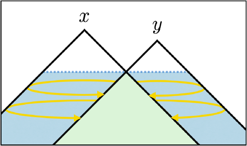
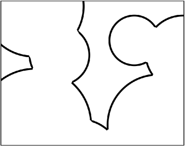
In a thermal first-order phase transition, true-vacuum bubbles start to nucleate at some temperature, and then they expand because of the pressure difference between the false and true vacua. These bubbles eventually collide with each other and the phase transition completes. Though uncollided bubbles do not radiate GWs because of the spherical symmetry of each bubble, the collision process breaks the symmetry and as a result GWs are produced. The analysis of GW production from such processes was initiated in Refs. [66, 67, 68, 69]. In the first numerical simulation carried out in Ref. [66] in a vacuum transition, it was noticed that the main GW production comes from the uncollided regions of the bubble walls. This observation made the basis for the “envelope approximation,” in which only the uncollided regions of the bubble walls are taken into account in calculating GW production (see Fig. 2). This approximation has been widely used in the subsequent literature together with the “thin-wall approximation,” in which the released energy is assumed to be concentrated in infinitely thin bubble walls.♢♢\diamondsuit1♢♢\diamondsuit1\diamondsuit1 Though in the early literature the envelope approximation includes the thin-wall approximation [66, 67, 68, 69], we distinguish them in this paper. Later a numerical simulation with the same approximations has been performed in Ref. [70] with an increased number of bubbles, and a more precise form of the GW spectrum has been obtained.

In the literature mentioned above, the bubble walls are thought to represent the energy concentration by the profile of the scalar field that drives the transition or by the bulk motion of the fluid coupled to the scalar field. It has recently been noticed in a series of numerical simulations [71, 72, 73]♢♢\diamondsuit2♢♢\diamondsuit2\diamondsuit2 See also Refs. [74, 75, 76] for other numerical simulations. that the latter bulk motion propagates even after bubble collisions, and works as a long-lasting source of GWs. It has been found that the GWs from such sound waves typically dominate the other sources of GWs,♢♢\diamondsuit3♢♢\diamondsuit3\diamondsuit3 In addition to bubble collisions and sound waves, turbulence is another important source for GWs [69, 77, 78, 79, 80, 81]. Note that the sound-wave regime as we study in this paper can develop into turbulent regime at late times. and that the resulting spectrum cannot be modeled by the envelope approximation because of the long-lasting nature of the source [71, 72, 73, 82].

These numerical simulations have brought significant developments in our understanding on GW sourcing both from bubble collisions and from sound waves. In this paper, however, we stress the importance of the cooperation between

  • Analytic understanding          &          Numerical understanding,

and aim to develop the former. This is partly because the former approach sometimes goes beyond the barrier of computational resources, and also because it often gives a clearer understanding of the system.♢♢\diamondsuit4♢♢\diamondsuit4\diamondsuit4 Note that another analytic modeling (sound-shell model [83]) has also been proposed to explain the enhancement of the GW spectrum around the scale of sound shell thickness. For this purpose we adopt the method of relating the GW spectrum with the two-point correlator of the energy-momentum tensor T(x)T(y)delimited-⟨⟩𝑇𝑥𝑇𝑦\left<T(x)T(y)\right>, which is pioneered in Ref. [84] in the context of GW production from bubble dynamics. In Ref. [85] it has been pointed out that, under the thin-wall approximation, various contributions to the correlator T(x)T(y)delimited-⟨⟩𝑇𝑥𝑇𝑦\left<T(x)T(y)\right> reduce to finite number of classes. This observation made it possible to write down the GW spectrum analytically in the same setup as the numerical study in Ref. [70], i.e. the GW spectrum with the thin-wall and envelope approximations.♢♢\diamondsuit5♢♢\diamondsuit5\diamondsuit5 By using the same formalism, it is also possible to investigate the effect of the bubble nucleation rate on the GW spectrum analytically [86]. In this paper we further develop this method, and write down

  • Gravitational-wave spectrum with the thin-wall approximation

    but without the envelope approximation.♢♢\diamondsuit6♢♢\diamondsuit6\diamondsuit6 There are other assumptions and approximations such as constant wall velocity, free propagation after collision and the absence of cosmic expansion: see Sec. 2.

As explained in Sec. 2, the bubble walls in our setup can be regarded as modeling the energy concentration in the scalar field and/or in the bulk motion of the fluid, and therefore the resulting spectrum is considered to be relevant to GW production both from bubble collisions (scalar field contribution) and sound waves (fluid contribution). We discuss the implications and also limitations of our modeling there. The analytic expressions for the GW spectrum, Eqs. (3.2) and (3.3), have multi-dimensional integrations, and therefore we evaluate them with numerical methods.♢♢\diamondsuit7♢♢\diamondsuit7\diamondsuit7 Note that this is essentially different from numerical simulations: the GW spectrum obtained this paper is the spectrum taking infinitely many bubbles into account. As a result, the growth and saturation of the spectrum are clearly observed as a function of the duration time of the collided walls.

The organization of the paper is as follows. In Sec. 2 we present our setup and summarize basic ingredients to estimate the GW spectrum. We also discuss the implications and limitations of our setup in this section. In Sec. 3 we write down the analytic expressions for the GW spectrum, and we evaluate them in Sec. 4 with Monte-Carlo integration. Sec. 5 is devoted to discussion and conclusions.

2 Setup and basic ingredients

In this section, we present our setup and basic ingredients to estimate the GW spectrum. In order to estimate the spectrum, we have to clarify the energy-momentum tensor of the system. It is determined by

  • (1)

    Spacetime distribution of bubbles (i.e. nucleation rate of bubbles),

  • (2)

    Energy-momentum tensor profile around a bubble wall,

  • (3)

    Dynamics after bubble collisions.

Since it is generically hard to solve the full dynamics of the system, reasonable approximations are necessary for practical calculations. The aim of the following subsections is to clarify our approximations and their validity.

In Sec. 2.1, we give a brief overview of bubble dynamics in a cosmological phase transition, and explain our approximations for (2) and (3). In this subsection we do not show the explicit expression for the energy-momentum profile in order to avoid possible complications. In Sec. 2.2, we present the explicit form of the profile. In Sec. 2.3, we give our assumption about the nucleation rate which determines (1). In Sec. 2.4, we present a formalism to calculate the GW spectrum from the correlation function of the energy-momentum tensor. In Sec. 2.5 we summarize our setup and discuss its physical implications.

Before moving on, we comment on the meaning of “wall” in the present paper. This word usually refers to the energy localization in the scalar field gradient. We use the word “scalar wall” for such energy localization throughout the paper. This is because, as mentioned in Sec. 1, the main energy carrier around bubbles can be not only the scalar field but also the bulk motion of the fluid. Since our modeling aims to represent (at least some aspects of) the scalar field and sound waves, we refer to the energy localization from both as “wall” after modeling the energy-momentum profile.

2.1 Bubble dynamics in cosmological phase transitions

In this subsection we give a brief overview of GW production in a cosmological phase transition paying particular attention to the bubble dynamics. We also introduce our approximations for (2) and (3) and discuss their validity.

Classification

In cosmological first-order phase transitions, bubbles of the true vacuum nucleate, expand and then collide with each other. The released free energy accumulates around the bubble surfaces during their expansion. Though uncollided bubbles do not radiate GWs because of the spherical symmetry of each bubble, their collisions break it and produce GWs. In order to estimate the resulting GW spectrum, we have to know the energy-momentum tensor of the system determined by the bubble dynamics. The behavior of the expanding bubbles can be categorized into three classes:

  • (a)

    Runaway,

  • (b)

    Low terminal velocity,

  • (c)

    High terminal velocity.

Roughly speaking, the balance between the released energy and the friction coming from the background thermal plasma determines which case is realized (see e.g. Refs. [87, 88]). Schematically, the acceleration of the scalar wall is given by

v˙wρ0Ffric(vw),proportional-tosubscript˙𝑣𝑤subscript𝜌0subscript𝐹fricsubscript𝑣𝑤\displaystyle\dot{v}_{w}\propto\rho_{0}-F_{\rm fric}(v_{w}), (2.1)

where vwsubscript𝑣𝑤v_{w} is the scalar wall velocity, ρ0subscript𝜌0\rho_{0} denotes the released energy, and Ffric(vw)subscript𝐹fricsubscript𝑣𝑤F_{\rm fric}(v_{w}) denotes the friction term.

In the non-relativistic regime, the friction term is proportional to the velocity: Ffricvwproportional-tosubscript𝐹fricsubscript𝑣𝑤F_{\rm fric}\propto v_{w}. If the ratio α𝛼\alpha between the released energy ρ0subscript𝜌0\rho_{0} and that of the surrounding plasma ρradsubscript𝜌rad\rho_{\rm rad}

α𝛼\displaystyle\alpha ρ0ρrad,absentsubscript𝜌0subscript𝜌rad\displaystyle\equiv\frac{\rho_{0}}{\rho_{\rm rad}}, (2.2)

is suppressed α𝒪(0.1)less-than-or-similar-to𝛼𝒪0.1\alpha\lesssim{\mathcal{O}}(0.1), the acceleration tends to cease within non-relativistic regime.♢♢\diamondsuit8♢♢\diamondsuit8\diamondsuit8 In order to determine the terminal velocity, we have to specify couplings between the scalar field and the plasma. Here we do not consider details of friction, assuming that the couplings are not extremely suppressed. We refer to such cases as (b) low terminal velocity. On the other hand, if the released energy is large enough α𝒪(0.1)greater-than-or-equivalent-to𝛼𝒪0.1\alpha\gtrsim{\mathcal{O}}(0.1), the scalar wall velocity enters the relativistic regime vw1similar-to-or-equalssubscript𝑣𝑤1v_{w}\simeq 1. In order to deal with this regime, we have to know the behavior of the friction term in γw1/1vw2subscript𝛾𝑤11superscriptsubscript𝑣𝑤2\gamma_{w}\equiv 1/\sqrt{1-v_{w}^{2}}\rightarrow\infty limit. Though it had long been considered that the friction saturates in the relativistic limit and cannot stop the acceleration of the scalar wall [89], the authors of Ref. [90] have recently pointed out that particle splitting processes around the wall generate a friction term proportional to γwsubscript𝛾𝑤\gamma_{w}. This term becomes larger and larger in γwsubscript𝛾𝑤\gamma_{w}\rightarrow\infty limit, and stops the acceleration before bubble collisions in some cases. In fact, as we discuss in Sec. 2.1 (c), the acceleration may stop due to this splitting process for most cases of our interest. We refer to such cases as (c) high terminal velocity. We also denote by (a) runaway those cases in which the acceleration continues all the way until bubble collisions.

As mentioned in the beginning of this section, in order to have the energy-momentum tensor of the system, we have to clarify

  • (2)

    Energy-momentum tensor profile around a bubble wall,

  • (3)

    Dynamics after bubble collisions,

for each of (a), (b) and (c). Especially, the importance of (3) has recently been pointed out in Refs. [71, 72, 73], in which the authors observed a sizable GW production from sound waves after bubble collisions. In this paper, we adopt

  • (2)

    Thin-wall approximation,

  • (3)

    Free propagation,

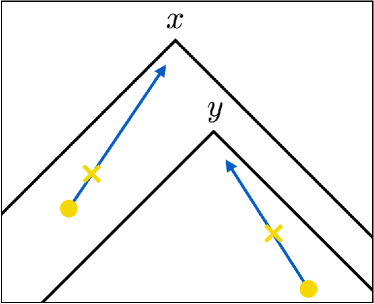
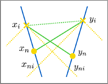
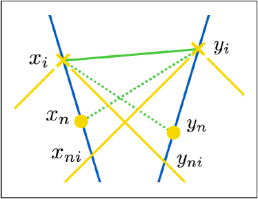
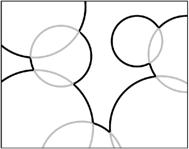
for these two. The former assumes that the released energy is localized in an infinitesimally thin surface of a bubble, while the latter assumes that the energy and momentum accumulated around the bubble surfaces until the first collision just pass through after that. See also Eq. (2.21) for the explicit form of the energy-momentum tensor. Fig. 2 is a schematic picture of the system with these approximations. The black lines denote the thin walls, which model the energy and momentum localization in the scalar wall and/or in the bulk motion of the fluid. The released energy accumulates until their first collisions. On the other hand, the gray lines denote the evolution of such localized energy and momentum after collisions. They gradually lose the accumulated energy and momentum densities after collisions, as a result of free propagation. In addition, we assume that the propagation velocity of such localized energy is constant both before and after collisions, and denote it by v𝑣v. Below we discuss the validity of such approximations (thin-wall and free propagation with a constant velocity) for both (a) and (b). Unfortunately, we do not know much about the dynamics realized in case (c). Thus, we only mention some features and possible procedures to determine the GW spectrum in this case. We summarize the properties of each case in Table 1.

Before moving on, we comment on turbulence after bubble collisions. In all of the three cases plasma turbulence can be a sizable source for GWs at late times [69, 77, 78, 79, 80, 81]. However, since the turbulence dynamics is highly nonlinear, we restrict ourselves to the bubble dynamics before the onset of turbulence in this paper.
Refer to caption
Figure 1: Rough sketch of the bubble dynamics with the envelope approximation. The bubble walls, denoted by the black lines, accumulate energy and momentum as they expand and then lose them instantly when they collide with each other. Compare this figure with Fig. 2. This figure is the same as in Ref. [85].
Refer to caption
Figure 2: Rough sketch of the bubble dynamics without the envelope approximation. The collided bubble walls, denoted by the gray lines, gradually lose their energy and momentum densities after collisions.
Table 1: Classification of bubble dynamics
Type Width of source Scalar wall velocity Dynamics after collision
Runaway thin γw1much-greater-thansubscript𝛾𝑤1\gamma_{w}\gg 1 free propagation with speed of light
Low terminal velocity thick constant vwsubscript𝑣𝑤v_{w} free propagation with speed of sound
High terminal velocity ? constant γw1much-greater-thansubscript𝛾𝑤1\gamma_{w}\gg 1 ?

(a) Runaway

In the runaway case the released energy is relatively large (α𝒪(0.1)greater-than-or-equivalent-to𝛼𝒪0.1\alpha\gtrsim{\mathcal{O}}(0.1)) and the friction term cannot stop the acceleration of the scalar wall by the time of collisions. Below we assume that the friction from the surrounding plasma, especially the splitting effect explained in (c) high terminal velocity, is negligible. We also assume that the energy density of the Universe is dominated by the vacuum energy density.♢♢\diamondsuit9♢♢\diamondsuit9\diamondsuit9 This is indeed a good assumption, since extremely large values of α𝛼\alpha are required for runaway walls: see the estimate in (c) High terminal velocity.

In the runaway case, the released energy accumulates around a thin surface of a bubble in the form of scalar gradient. Let us first consider the behavior of the scalar field before collisions. Suppose that the scalar field difference between the true and false vacua is ΔϕΔitalic-ϕ\Delta\phi, the released energy density is ρ0subscript𝜌0\rho_{0}, the bubble radius is R𝑅R, and the width of energy localization is lbsubscript𝑙𝑏l_{b}. We may estimate the width of the surface as

(Δϕlb)2lbR2superscriptΔitalic-ϕsubscript𝑙𝑏2subscript𝑙𝑏superscript𝑅2\displaystyle\left(\frac{\Delta\phi}{l_{b}}\right)^{2}l_{b}R^{2} ρ0R3lbΔϕ2ρ0R.formulae-sequencesimilar-toabsentsubscript𝜌0superscript𝑅3similar-tosubscript𝑙𝑏Δsuperscriptitalic-ϕ2subscript𝜌0𝑅\displaystyle\sim\rho_{0}R^{3}\;\;\;\;\to\;\;\;\;l_{b}\sim\frac{\Delta\phi^{2}}{\rho_{0}R}. (2.3)

We see that the scalar wall becomes thiner and thiner as the bubble expands. As we see in Sec. 2.3, the typical bubble size just before collision is sub-horizon, which we denote Rcoll=ϵ/Hsubscript𝑅collitalic-ϵ𝐻R_{\rm coll}=\epsilon/H with ϵ𝒪(0.1)less-than-or-similar-toitalic-ϵ𝒪0.1\epsilon\lesssim{\mathcal{O}}(0.1) with H𝐻H denoting the Hubble parameter. For clarity, we parametrize ρ0subscript𝜌0\rho_{0} as ρ0mtyp2Δϕ2similar-tosubscript𝜌0superscriptsubscript𝑚typ2Δsuperscriptitalic-ϕ2\rho_{0}\sim m_{\rm typ}^{2}\Delta\phi^{2} where mtypsubscript𝑚typm_{\rm typ} denotes the typical mass scale of the potential. Usually mtypTsimilar-tosubscript𝑚typ𝑇m_{\rm typ}\sim T holds with T𝑇T being the temperature of the plasma around the time of transition. Also mtypTΔϕsimilar-tosubscript𝑚typ𝑇less-than-or-similar-toΔitalic-ϕm_{\rm typ}\sim T\lesssim\Delta\phi holds for most of the runaway cases since the released energy dominates the radiation energy. The typical momentum kbsubscript𝑘𝑏k_{b} of the scalar field configuration just before collision is given by

kbsubscript𝑘𝑏\displaystyle k_{b} 1lb|R=RcollϵMP(mtypΔϕ),similar-toabsentevaluated-at1subscript𝑙𝑏𝑅subscript𝑅collsimilar-toitalic-ϵsubscript𝑀𝑃subscript𝑚typΔitalic-ϕ\displaystyle\sim\left.\frac{1}{l_{b}}\right|_{R=R_{\rm coll}}\sim\epsilon M_{P}\left(\frac{m_{\rm typ}}{\Delta\phi}\right), (2.4)

where MPsubscript𝑀𝑃M_{P} denotes the reduced Planck mass and we used the Friedmann equation MP2H2ρ0similar-tosuperscriptsubscript𝑀𝑃2superscript𝐻2subscript𝜌0M_{P}^{2}H^{2}\sim\rho_{0} satisfied in the runaway case. Note that the typical momentum is much larger than other physical parameters such as mtypsubscript𝑚typm_{\rm typ} as long as the phase transition occurs well below the Planck scale. In particle analogy, the number density nbsubscript𝑛𝑏n_{b} of such high momentum modes just before collision is given by

kbnblbRcoll2subscript𝑘𝑏subscript𝑛𝑏subscript𝑙𝑏superscriptsubscript𝑅coll2\displaystyle k_{b}n_{b}l_{b}R_{\rm coll}^{2} ρ0Rcoll3nbϵMPmtypΔϕ.formulae-sequencesimilar-toabsentsubscript𝜌0superscriptsubscript𝑅coll3similar-tosubscript𝑛𝑏italic-ϵsubscript𝑀𝑃subscript𝑚typΔitalic-ϕ\displaystyle\sim\rho_{0}R_{\rm coll}^{3}\;\;\;\;\rightarrow\;\;\;\;n_{b}\sim\epsilon M_{P}m_{\rm typ}\Delta\phi. (2.5)

Now let us consider the effect of bubble collisions, assuming that the particle analogy is applicable. We focus only on those high momentum modes where most of the released energy is accumulated. Though the scalar field profile is deformed to some extent during the collision process, deformation in such high momentum modes is expected to be small. To see this, let us consider a scattering process caused by λϕ4𝜆superscriptitalic-ϕ4\lambda\phi^{4} interaction for example. Denoting the change in the number density of such high momentum modes by ΔnbΔsubscript𝑛𝑏\Delta n_{b}, we have the following relation:

ΔnbnbΔsubscript𝑛𝑏subscript𝑛𝑏\displaystyle\frac{\Delta n_{b}}{n_{b}} λ2kb2nbΔtcoll,Δtcoll1lbΔnbnbλ2ϵ2(Δϕmtyp)(HMP)1,formulae-sequencesimilar-toabsentsuperscript𝜆2superscriptsubscript𝑘𝑏2subscript𝑛𝑏Δsubscript𝑡collformulae-sequencesimilar-toΔsubscript𝑡coll1subscript𝑙𝑏similar-toΔsubscript𝑛𝑏subscript𝑛𝑏superscript𝜆2superscriptitalic-ϵ2Δitalic-ϕsubscript𝑚typ𝐻subscript𝑀𝑃much-less-than1\displaystyle\sim\frac{\lambda^{2}}{k_{b}^{2}}n_{b}\Delta t_{\rm coll},\;\;\;\;\Delta t_{\rm coll}\sim\frac{1}{l_{b}}\;\;\;\;\rightarrow\;\;\;\;\frac{\Delta n_{b}}{n_{b}}\sim\frac{\lambda^{2}}{\epsilon^{2}}\left(\frac{\Delta\phi}{m_{\rm typ}}\right)\left(\frac{H}{M_{P}}\right)\ll 1, (2.6)

with ΔtcollΔsubscript𝑡coll\Delta t_{\rm coll} indicating the duration time of the collision process. We see that the effect of collision is typically negligible for the high momentum modes because of the last factor.

Next let us consider the effect of decay processes after bubble collisions. Denoting the mass and decay rate of the scalar field at the true vacuum by mtypsimilar-toabsentsubscript𝑚typ\sim m_{\rm typ} and y2mtypsimilar-toabsentsuperscript𝑦2subscript𝑚typ\sim y^{2}m_{\rm typ}, respectively, we may estimate the lifetime of high momentum modes ΔtdecayΔsubscript𝑡decay\Delta t_{\rm decay} as

HΔtdecay𝐻Δsubscript𝑡decay\displaystyle H\Delta t_{\rm decay} mtypΔϕMP1y2mtypkbmtypϵy2.similar-toabsentsubscript𝑚typΔitalic-ϕsubscript𝑀𝑃1superscript𝑦2subscript𝑚typsubscript𝑘𝑏subscript𝑚typsimilar-toitalic-ϵsuperscript𝑦2\displaystyle\sim\frac{m_{\rm typ}\Delta\phi}{M_{P}}\frac{1}{y^{2}m_{\rm typ}}\frac{k_{b}}{m_{\rm typ}}\sim\frac{\epsilon}{y^{2}}. (2.7)

Therefore the lifetime can be comparable to the Hubble time though it depends on the model parameters.

Finally let us consider the validity of the thin-wall approximation after collisions. After bubbles collide with each other, the energy injection into the scalar motion ceases and the scalar field start to evolve with free propagation. Since the scalar motion has a finite momentum width ΔkbΔsubscript𝑘𝑏\Delta k_{b}, the width of the energy concentration becomes thicker and thicker. On the other hand, the relevant scale in the GW spectrum is the typical bubble size around the time of collisions. Therefore, the thin-wall approximation is expected to hold until the width of the energy concentration becomes comparable to this length scale. Let us denote by ΔtthinΔsubscript𝑡thin\Delta t_{\rm thin} the timescale with which the scalar wall width grows to this length scale. Approximating the momentum width by Δkbkbsimilar-toΔsubscript𝑘𝑏subscript𝑘𝑏\Delta k_{b}\sim k_{b}, we may estimate ΔtthinΔsubscript𝑡thin\Delta t_{\rm thin} as

ΔtthinΔvwΔsubscript𝑡thinΔsubscript𝑣𝑤\displaystyle\Delta t_{\rm thin}\Delta v_{w} RcollHΔtthinϵ(kbmtyp)21,formulae-sequencesimilar-toabsentsubscript𝑅collsimilar-to𝐻Δsubscript𝑡thinitalic-ϵsuperscriptsubscript𝑘𝑏subscript𝑚typ2much-greater-than1\displaystyle\sim R_{\rm coll}\;\;\;\;\rightarrow\;\;\;\;H\Delta t_{\rm thin}\sim\epsilon\left(\frac{k_{b}}{m_{\rm typ}}\right)^{2}\gg 1, (2.8)

with ΔvwΔsubscript𝑣𝑤\Delta v_{w} being the velocity dispersion corresponding to ΔkbΔsubscript𝑘𝑏\Delta k_{b}.♢♢\diamondsuit10♢♢\diamondsuit10\diamondsuit10 This can be estimated from the relation between the velocity dispersion and the momentum dispersion: ΔγwΔsubscript𝛾𝑤\displaystyle\Delta\gamma_{w} vwΔvw(1vw2)3/2ΔkbmtypkbmtypΔvw1γw3kbmtypmtyp2kb2.similar-toabsentsubscript𝑣𝑤Δsubscript𝑣𝑤superscript1superscriptsubscript𝑣𝑤232similar-toΔsubscript𝑘𝑏subscript𝑚typsimilar-tosubscript𝑘𝑏subscript𝑚typΔsubscript𝑣𝑤similar-to1superscriptsubscript𝛾𝑤3subscript𝑘𝑏subscript𝑚typsimilar-tosuperscriptsubscript𝑚typ2superscriptsubscript𝑘𝑏2\displaystyle\sim\frac{v_{w}\Delta v_{w}}{(1-v_{w}^{2})^{3/2}}\sim\frac{\Delta k_{b}}{m_{\rm typ}}\sim\frac{k_{b}}{m_{\rm typ}}~{}~{}\to~{}~{}\Delta v_{w}\sim\frac{1}{\gamma_{w}^{3}}\frac{k_{b}}{m_{\rm typ}}\sim\frac{m_{\rm typ}^{2}}{k_{b}^{2}}. (2.9) Hence, the thin-wall approximation can be valid until a Hubble time as long as the phase transition occurs much below the Planck scale.

Let us summarize the runaway case. During bubble expansion, the released energy accumulates within extremely thin regions in the form of scalar gradient, and the scalar field becomes ultra-relativistic. As long as particle analogy is applicable, the effect of bubble collisions is typically negligible for such ultra-relativistic modes, and the scalar walls are almost luminal both before and after collisions.♢♢\diamondsuit11♢♢\diamondsuit11\diamondsuit11 Note that, if nontrivial trapping of the scalar field at the false vacuum occurs after collisions, the dynamics can be quite different from the one described here [91]. Though it should be confirmed in future studies that the above particle analogy is applicable in a system with extremely relativistic scalar configurations γw1much-greater-thansubscript𝛾𝑤1\gamma_{w}\gg 1,♢♢\diamondsuit12♢♢\diamondsuit12\diamondsuit12 Note that numerical simulations with γw1much-greater-thansubscript𝛾𝑤1\gamma_{w}\gg 1, which is relevant in the runaway case, are generically difficult. it is at least expected that the scalar field configurations are still energetic for some time after collisions.

(b) Low terminal velocity

Next let us consider those cases where the released energy is subdominant compared to that of radiation (α𝒪(0.1)less-than-or-similar-to𝛼𝒪0.1\alpha\lesssim{\mathcal{O}}(0.1)). In such cases, the dynamics of bubble expansion is determined by coupled equations between the scalar field and the plasma. Soon after bubbles nucleate, the pressure difference between the true and false vacua gets balanced with the friction from the thermal plasma, and as a result the scalar wall velocity vwsubscript𝑣𝑤v_{w} approaches a constant value [87].

During bubble expansion, the released energy is converted into the bulk motion of the plasma surrounding the scalar wall. Since there is no distance scale in the fluid equations, the fluid profile (enthalpy ω𝜔\omega, fluid velocity u𝑢\vec{u}, and so on) depends only on the variable ξr/t𝜉𝑟𝑡\xi\equiv r/t, where r𝑟r is the distance from the bubble nucleation point and t𝑡t is the time after nucleation. Generally the fluid bulk motion is localized around the position of the scalar wall ξvwsimilar-to𝜉subscript𝑣𝑤\xi\sim v_{w},♢♢\diamondsuit13♢♢\diamondsuit13\diamondsuit13 Note that this does not necessarily mean that the fluid velocity u𝑢u is close to the scalar wall velocity vwsubscript𝑣𝑤v_{w}. and the width of this energy localization is smaller than but comparable to the bubble size. The fraction κ𝜅\kappa, called the efficiency factor, is defined as the fraction of the released energy ρ0subscript𝜌0\rho_{0} which goes into the plasma motion. It is obtained from the velocity and enthalpy profile as [87]

κ𝜅\displaystyle\kappa =3ρ0vw30𝑑ξξ2ωγ2u2,absent3subscript𝜌0superscriptsubscript𝑣𝑤3superscriptsubscript0differential-d𝜉superscript𝜉2𝜔superscript𝛾2superscript𝑢2\displaystyle=\frac{3}{\rho_{0}v_{w}^{3}}\int_{0}^{\infty}d\xi~{}\xi^{2}\omega\gamma^{2}u^{2}, (2.10)

with γ1/1u2𝛾11superscript𝑢2\gamma\equiv 1/\sqrt{1-u^{2}} and u|u|𝑢𝑢u\equiv|\vec{u}|.

After the bubbles collide, the energy injection into plasma motion ceases. However, as pointed out in Refs. [71, 72, 73], the plasma motion remains after bubble collisions and produce a sizable amount of GWs. In the present case the released energy is typically subdominant compared to the plasma energy density, and thus δρ/ρrad1much-less-than𝛿𝜌subscript𝜌rad1\delta\rho/\rho_{\rm rad}\ll 1 and u1much-less-than𝑢1u\ll 1 hold in most cases with δρκρ0similar-to𝛿𝜌𝜅subscript𝜌0\delta\rho\sim\kappa\rho_{0} being the energy density in the plasma motion localized around the bubbles. When these two conditions hold, the dynamics of the plasma motion is well described by linear theory (sound wave dynamics). For example, the fluid velocity obeys the ordinary wave equation

(2t2cs2Δ)usuperscript2superscript𝑡2superscriptsubscript𝑐𝑠2Δ𝑢\displaystyle\left(\frac{\partial^{2}}{\partial t^{2}}-c_{s}^{2}\Delta\right)\vec{u} =0,absent0\displaystyle=0, (2.11)

with cs1/3similar-to-or-equalssubscript𝑐𝑠13c_{s}\simeq 1/\sqrt{3} being the speed of sound. Therefore the plasma dynamics after bubble collisions is described just by the free propagation of plasma motions with the speed of sound. The width of the energy localization is fixed at the first collision, and the plasma velocity u𝑢u starts to decrease after that because of the increase in the volume of energy localization and because of the energy conservation.♢♢\diamondsuit14♢♢\diamondsuit14\diamondsuit14 On this point our modeling of the system differs from the one in Ref. [84]. Though sound waves might be damped by viscosity at late times, the timescale of such an effect can be larger than the Hubble time [73].

In short, the bubble dynamics in the low terminal velocity case is as follows: during bubble expansion the released energy is converted into the plasma bulk motion around bubbles within relatively thick regions (compared to (a) runaway case), while after bubble collisions the fluid motions obey simple wave equations and they freely propagate with the speed of sound cssubscript𝑐𝑠c_{s}.

Now let us discuss the validity of our assumptions, i.e. thin-wall and free propagation with a constant velocity v𝑣v. For the thin-wall approximation, as long as we are interested in frequencies corresponding to length scales around or larger than the typical bubble size, we expect that the thin-wall approximation works as a reasonable approximation because such modes cannot see the width of the energy concentration.♢♢\diamondsuit15♢♢\diamondsuit15\diamondsuit15 One might worry that the thin-wall approximation may fail to describe the present system after the region of energy localization fills the whole Universe. (Note that the volume of energy localization continues to increase after bubble collisions.) See the discussion in the latter part of Sec. 5 on this point. However, for length scales around or smaller than the thickness of energy localization, our modeling misses an important contribution from superpositions of fluid velocity.♢♢\diamondsuit16♢♢\diamondsuit16\diamondsuit16 In fact, in the sound-shell model [83], it is the overlap of sound shells that contributes to the continuous GW sourcing. Therefore, our modeling should be regarded as capturing possible infrared structure in the GW spectrum. Regarding free propagation after collisions, it is justified as long as the fluid obeys the ordinary wave equation. On the other hand, the assumption of a constant velocity may fail in some cases, because the velocity in the present case is not unique: the region of energy concentration expands with a velocity around ξvwsimilar-to𝜉subscript𝑣𝑤\xi\sim v_{w} before collisions, while it propagates with the speed of sound cssubscript𝑐𝑠c_{s} after collisions. However, as long as vwcs𝒪(0.1)similar-to-or-equalssubscript𝑣𝑤subscript𝑐𝑠similar-to𝒪0.1v_{w}\simeq c_{s}\sim\mathcal{O}(0.1), our modeling is expected to work as a reasonable estimate for the infrared structure by setting the velocity v𝑣v to be cssubscript𝑐𝑠c_{s}.♢♢\diamondsuit17♢♢\diamondsuit17\diamondsuit17 Note that phase transitions with vw𝒪(0.1)greater-than-or-equivalent-tosubscript𝑣𝑤𝒪0.1v_{w}\gtrsim\mathcal{O}(0.1) is most relevant from the viewpoint of detection, because otherwise GW production is suppressed. To summarize, our setup will work as a reasonable estimate on the GW spectrum for low frequencies (around or lower than the inverse of the typical bubble size at the collision time) as long as vw𝒪(0.1)similar-tosubscript𝑣𝑤𝒪0.1v_{w}\sim\mathcal{O}(0.1).

(c) High terminal velocity

Finally let us discuss the high terminal velocity case. Recently, the authors of Ref. [90] have pointed out that particle splitting processes generate a friction term proportional to γwsubscript𝛾𝑤\gamma_{w}. We denote by (c) high terminal velocity those cases in which such a friction term stops the acceleration of the bubble walls before collisions. Below we discuss when this is realized instead of (a) runaway. We also mention the behavior of the energy-momentum tensor.

First let us consider when (c) is realized by estimating the terminal velocity in (a) and (c). The friction term from the particle splitting processes is given by [90]

Ffric(vw)subscript𝐹fricsubscript𝑣𝑤\displaystyle F_{\rm fric}(v_{w}) γwgtyp2ΔmT3,similar-toabsentsubscript𝛾𝑤superscriptsubscript𝑔typ2Δ𝑚superscript𝑇3\displaystyle\sim\gamma_{w}g_{\rm typ}^{2}\Delta{m}T^{3}, (2.12)

where gtypsubscript𝑔typg_{\rm typ} denotes a typical value of the coupling of such species to the scalar field, and ΔmΔ𝑚\Delta m denotes the mass of some particle species gained by the transition from the false to the true vacuum. This friction term stops the acceleration of the wall when Ffricsubscript𝐹fricF_{\rm fric} becomes comparable to ρ0subscript𝜌0\rho_{0}, which gives

γwhighterminalsuperscriptsubscript𝛾𝑤highterminal\displaystyle\gamma_{w}^{\rm high-terminal} αgtyp2(TΔm).similar-toabsent𝛼superscriptsubscript𝑔typ2𝑇Δ𝑚\displaystyle\sim\frac{\alpha}{g_{\rm typ}^{2}}\left(\frac{T}{\Delta m}\right). (2.13)

On the other hand, if we assume runaway, the wall continues to be accelerated until collision, and γwsubscript𝛾𝑤\gamma_{w} becomes

γwrunawaysuperscriptsubscript𝛾𝑤runaway\displaystyle\gamma_{w}^{\rm runaway} ϵ(MPΔϕ).similar-toabsentitalic-ϵsubscript𝑀𝑃Δitalic-ϕ\displaystyle\sim\epsilon\left(\frac{M_{P}}{\Delta\phi}\right). (2.14)

The condition for runaway is then written as γwrunawayγwhighterminalless-than-or-similar-tosuperscriptsubscript𝛾𝑤runawaysuperscriptsubscript𝛾𝑤highterminal\gamma_{w}^{\rm runaway}\lesssim\gamma_{w}^{\rm high-terminal}, which gives

α𝛼\displaystyle\alpha ϵgtyp2(ΔmΔϕ)(MPT).greater-than-or-equivalent-toabsentitalic-ϵsuperscriptsubscript𝑔typ2Δ𝑚Δitalic-ϕsubscript𝑀𝑃𝑇\displaystyle\gtrsim\epsilon g_{\rm typ}^{2}\left(\frac{\Delta m}{\Delta\phi}\right)\left(\frac{M_{P}}{T}\right). (2.15)

Therefore, runaway seems unlikely unless a huge amount of latent heat is released in the transition.

Now let us consider the behavior of the energy-momentum tensor. Before bubble collisions, the released energy is converted into the plasma bulk motion localized around the scalar walls.♢♢\diamondsuit18♢♢\diamondsuit18\diamondsuit18 The situation near the scalar walls may be far from thermal equilibrium because of the production of energetic particles. However, the fluid description is still expected to be valid for the length scale relevant to GW production Rcollϵ/Hsimilar-tosubscript𝑅collitalic-ϵ𝐻R_{\rm coll}\sim\epsilon/H, which is much larger than the typical length scale of particle scattering. Note that in the present case the energy localization is much thinner than (b) low terminal velocity case [87]. Therefore, the thin-wall approximation is valid at least until the time of bubble collisions. However, because of the huge energy release, the energy density around the bubble surfaces is much larger than that of background δρ/ρrad1much-greater-than𝛿𝜌subscript𝜌rad1\delta\rho/\rho_{\rm rad}\gg 1, and the velocity field u𝑢u is no more nonrelativistic. Therefore, the fluid dynamics enters the nonlinear regime, and full numerical simulations are necessary in order to obtain the behavior of the energy-momentum tensor during and after bubble collisions. Such a study is beyond the scope of this paper.

2.2 Explicit form of the energy-momentum tensor

So far we have discussed the validity of our assumptions (thin-wall approximation and free propagation with a constant velocity). In this subsection we present the explicit form of the energy-momentum tensor we use in the following. The final expression is Eq. (2.16) with ρBsubscript𝜌𝐵\rho_{B} given by Eq. (2.21).

Thin-wall approximation

We first give the explicit form of the energy-momentum tensor for uncollided bubble walls to illustrate the thin-wall approximation. Here note that “walls” refer to the energy concentration by the scalar field gradient and/or the bulk motion of the fluid, as mentioned just before Sec. 2.1. Let us consider a setup where a single bubble nucleates at a spacetime point xn(txn,xn)subscript𝑥𝑛subscript𝑡𝑥𝑛subscript𝑥𝑛x_{n}\equiv(t_{xn},\vec{x}_{n}) and expands with a constant velocity v𝑣v, and denote the infinitesimal width of bubble walls by lBsubscript𝑙𝐵l_{B}. Here the subscript “n𝑛n” denotes “nucleation.” In this setup, the ij𝑖𝑗ij-part of the energy-momentum tensor TBsubscript𝑇𝐵T_{B} of this bubble is given by♢♢\diamondsuit19♢♢\diamondsuit19\diamondsuit19 Though in general there are isotropic contributions δijproportional-toabsentsubscript𝛿𝑖𝑗\propto\delta_{ij} from the false vacuum energy, we can neglect them because it does not contribute to GW production.

TBij(x)subscript𝑇𝐵𝑖𝑗𝑥\displaystyle T_{Bij}(x) =ρB(x)(xxn)^i(xxn)^j,absentsubscript𝜌𝐵𝑥subscript^𝑥subscript𝑥𝑛𝑖subscript^𝑥subscript𝑥𝑛𝑗\displaystyle=\rho_{B}(x)\widehat{(x-x_{n})}_{i}\widehat{(x-x_{n})}_{j}, (2.16)

with ρBsubscript𝜌𝐵\rho_{B} being ρB(uncollided)superscriptsubscript𝜌𝐵uncollided\rho_{B}^{\rm(uncollided)} defined as

ρB(uncollided)(x)superscriptsubscript𝜌𝐵uncollided𝑥\displaystyle\rho_{B}^{\rm(uncollided)}(x) {4π3rB(tx,txn)3κρ0/4πrB(tx,txn)2lBrB(tx,txn)<|xxn|<rB(tx,txn)0otherwise,absentcases4𝜋3subscript𝑟𝐵superscriptsubscript𝑡𝑥subscript𝑡𝑥𝑛3𝜅subscript𝜌04𝜋subscript𝑟𝐵superscriptsubscript𝑡𝑥subscript𝑡𝑥𝑛2subscript𝑙𝐵subscript𝑟𝐵subscript𝑡𝑥subscript𝑡𝑥𝑛𝑥subscript𝑥𝑛subscriptsuperscript𝑟𝐵subscript𝑡𝑥subscript𝑡𝑥𝑛0otherwise\displaystyle\equiv\left\{\begin{array}[]{cc}\displaystyle\frac{4\pi}{3}r_{B}(t_{x},t_{xn})^{3}\kappa\rho_{0}\Big{/}4\pi r_{B}(t_{x},t_{xn})^{2}l_{B}&r_{B}(t_{x},t_{xn})<|\vec{x}-\vec{x}_{n}|<r^{\prime}_{B}(t_{x},t_{xn})\\ 0&{\rm otherwise}\end{array}\right., (2.19)

and rB,rBsubscript𝑟𝐵subscriptsuperscript𝑟𝐵r_{B},r^{\prime}_{B} denoting the bubble radius

rB(tx,txn)subscript𝑟𝐵subscript𝑡𝑥subscript𝑡𝑥𝑛\displaystyle r_{B}(t_{x},t_{xn}) =v(txtxn),rB(tx,txn)=rB(tx,txn)+lB.formulae-sequenceabsent𝑣subscript𝑡𝑥subscript𝑡𝑥𝑛subscriptsuperscript𝑟𝐵subscript𝑡𝑥subscript𝑡𝑥𝑛subscript𝑟𝐵subscript𝑡𝑥subscript𝑡𝑥𝑛subscript𝑙𝐵\displaystyle=v(t_{x}-t_{xn}),\;\;\;r^{\prime}_{B}(t_{x},t_{xn})=r_{B}(t_{x},t_{xn})+l_{B}. (2.20)

Here x𝑥x denotes the spacetime point x=(tx,x)𝑥subscript𝑡𝑥𝑥x=(t_{x},\vec{x}), the Latin indices run over 1,2,31231,2,3 throughout the paper, and the hat on the vector ^^\hat{\bullet} indicates the unit vector in \vec{\bullet} direction. Also, as mentioned before, the efficiency factor κ𝜅\kappa is the fraction of the released energy density ρ0subscript𝜌0\rho_{0} localized around the walls♢♢\diamondsuit20♢♢\diamondsuit20\diamondsuit20 This corresponds to the energy of the bulk fluid when the scalar wall reaches a terminal velocity, while it corresponds to the energy of the scalar wall itself when the scalar field carries most of the released energy.  [69]. In the runaway case we have κ1similar-to-or-equals𝜅1\kappa\simeq 1, while in the terminal velocity cases it depends on the setup (see Eq. (2.10) and Refs. [87, 88]).

Free propagation with arbitrary damping

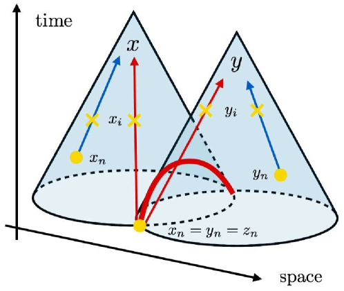
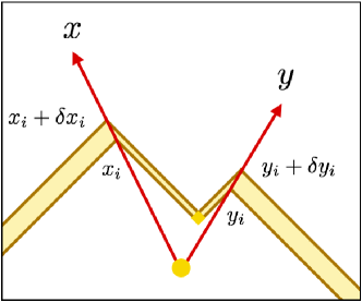
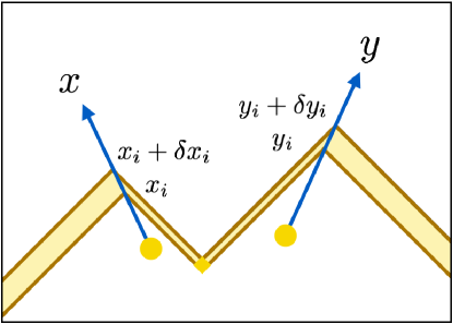
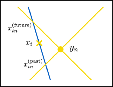
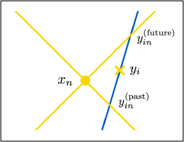
Now we give the explicit form of the energy-momentum tensor after collisions. Let us consider a bubble wall fragment which experiences the first collision at xi=(txi,xi)subscript𝑥𝑖subscript𝑡𝑥𝑖subscript𝑥𝑖x_{i}=(t_{xi},\vec{x}_{i}). In the following we often call this first collision “interception,” and label it by the subscript “i𝑖i.” Note that the interception point differs among each fragment. Assuming free propagation of the walls after the first collisions, we write ρB(x)subscript𝜌𝐵𝑥\rho_{B}(x) for this particular fragment after the first collision as

ρB(collided)(x)superscriptsubscript𝜌𝐵collided𝑥\displaystyle\rho_{B}^{({\rm collided})}(x) =[4π3rB(txi,txn)3κρ0/4πrB(txi,txn)2lB]×rB(txi,txn)2rB(tx,txn)2×D(tx,txi)absentdelimited-[]4𝜋3subscript𝑟𝐵superscriptsubscript𝑡𝑥𝑖subscript𝑡𝑥𝑛3𝜅subscript𝜌04𝜋subscript𝑟𝐵superscriptsubscript𝑡𝑥𝑖subscript𝑡𝑥𝑛2subscript𝑙𝐵subscript𝑟𝐵superscriptsubscript𝑡𝑥𝑖subscript𝑡𝑥𝑛2subscript𝑟𝐵superscriptsubscript𝑡𝑥subscript𝑡𝑥𝑛2𝐷subscript𝑡𝑥subscript𝑡𝑥𝑖\displaystyle=\displaystyle\left[\frac{4\pi}{3}r_{B}(t_{xi},t_{xn})^{3}\kappa\rho_{0}\Big{/}4\pi r_{B}(t_{xi},t_{xn})^{2}l_{B}\right]\times\frac{r_{B}(t_{xi},t_{xn})^{2}}{r_{B}(t_{x},t_{xn})^{2}}\times D(t_{x},t_{xi}) (2.21)
=ρB(uncollided)(x)×rB(txi,txn)3rB(tx,txn)3×D(tx,txi),absentsuperscriptsubscript𝜌𝐵uncollided𝑥subscript𝑟𝐵superscriptsubscript𝑡𝑥𝑖subscript𝑡𝑥𝑛3subscript𝑟𝐵superscriptsubscript𝑡𝑥subscript𝑡𝑥𝑛3𝐷subscript𝑡𝑥subscript𝑡𝑥𝑖\displaystyle=\rho_{B}^{({\rm uncollided})}(x)\times\frac{r_{B}(t_{xi},t_{xn})^{3}}{r_{B}(t_{x},t_{xn})^{3}}\times D(t_{x},t_{xi}), (2.22)

for rB(tx,txn)<|xxn|<rB(tx,txn)subscript𝑟𝐵subscript𝑡𝑥subscript𝑡𝑥𝑛𝑥subscript𝑥𝑛subscriptsuperscript𝑟𝐵subscript𝑡𝑥subscript𝑡𝑥𝑛r_{B}(t_{x},t_{xn})<|\vec{x}-\vec{x}_{n}|<r^{\prime}_{B}(t_{x},t_{xn}), while it vanishes otherwise. Note that we take only the first collisions into account and neglect the effect of subsequent collisions on the energy-momentum tensor. The second factor in the R.H.S. of Eq. (2.21) takes into account the increase in the wall area and the total energy conservation. Here we have introduced a “damping function” D𝐷D, which satisfies D(tx,txi=tx)=1𝐷subscript𝑡𝑥subscript𝑡𝑥𝑖subscript𝑡𝑥1D(t_{x},t_{xi}=t_{x})=1. This function accounts for how the collided walls lose their energy and momentum densities from txisubscript𝑡𝑥𝑖t_{xi} to txsubscript𝑡𝑥t_{x} in addition to the second factor in Eq. (2.21). For free propagation we have D=1𝐷1D=1 for an arbitrary combination of txsubscript𝑡𝑥t_{x} and txisubscript𝑡𝑥𝑖t_{xi}. Though our analytic expressions for the GW spectrum are applicable to any form of D𝐷D,♢♢\diamondsuit21♢♢\diamondsuit21\diamondsuit21 The dumping function D𝐷D depends on the underlying particle model which describes the strength of the coupling of the scalar field with light particles. As discussed in Sec. 2.1, in some cases we expect D1similar-to-or-equals𝐷1D\simeq 1 during one Hubble time. Though it may also depend on the nucleation time tnsubscript𝑡𝑛t_{n}, our final expressions for the GW spectrum can be applied to such cases as well. we adopt the following form for practical calculations:

D(t,ti)𝐷𝑡subscript𝑡𝑖\displaystyle D(t,t_{i}) =e(tti)/τ.absentsuperscript𝑒𝑡subscript𝑡𝑖𝜏\displaystyle=e^{-(t-t_{i})/\tau}. (2.23)

Here τ𝜏\tau denotes a typical damping timescale of the walls, which generally depends on the underlying particle model. The instant damping τ=0𝜏0\tau=0 corresponds to the envelope approximation (see Fig. 2), while τ=𝜏\tau=\infty corresponds to free propagation, i.e. no damping. The introduction of the damping function makes it possible to clarify when GWs are sourced for each wavenumber, as we see in Sec. 4.

Note that Eq. (2.21) reduces to Eq. (2.19) for txi=txsubscript𝑡𝑥𝑖subscript𝑡𝑥t_{xi}=t_{x}. Therefore, Eq. (2.16) with ρBsubscript𝜌𝐵\rho_{B} given by Eq. (2.21) (for uncollided walls we take txi=txsubscript𝑡𝑥𝑖subscript𝑡𝑥t_{xi}=t_{x}) is our assumption for the energy-momentum tensor.

2.3 Nucleation rate of bubbles

As mentioned in the beginning of this section, we need

  • (1)

    Spacetime distribution of bubbles (i.e., nucleation rate of bubbles),

in order to estimate the GW spectrum. In this paper we assume the following form for the bubble nucleation rate per unit time and volume:

Γ(t)Γ𝑡\displaystyle\Gamma(t) =Γeβ(tt),absentsubscriptΓsuperscript𝑒𝛽𝑡subscript𝑡\displaystyle=\Gamma_{*}e^{\beta(t-t_{*})}, (2.24)

where tsubscript𝑡t_{*} denotes some typical time for bubble nucleation, ΓsubscriptΓ\Gamma_{*} indicates the nucleation rate at t=t𝑡subscript𝑡t=t_{*}, and β𝛽\beta is assumed to be constant. The typical nucleation time tsubscript𝑡t_{*} is calculated from the condition H4Γ1similar-tosuperscriptsubscript𝐻4subscriptΓ1H_{*}^{4}\Gamma_{*}\sim 1 with Hsubscript𝐻H_{*} being the Hubble parameter at t=t𝑡subscript𝑡t=t_{*}, and this is equivalent to specifying the temperature Tsubscript𝑇T_{*} just before the nucleation time. The expression (2.24) applies to thermal phase transitions,♢♢\diamondsuit22♢♢\diamondsuit22\diamondsuit22 Those cases in which this expression does not hold have recently been studied by the authors of Ref. [92]. and the parameter β𝛽\beta is calculated with the instanton method from the underlying particle model [93, 94]. The inverse of β𝛽\beta gives a typical timescale from nucleation to collision, and the typical bubble size when bubbles collide (or the typical distance between two neighboring bubbles) is given by v/βsimilar-toabsent𝑣𝛽\sim v/\beta correspondingly.♢♢\diamondsuit23♢♢\diamondsuit23\diamondsuit23 This is understood as follows. The nucleation rate grows with a typical timescale 1/βsimilar-toabsent1𝛽\sim 1/\beta. This means that, after bubbles start to fill the Universe, they can expand only for a timescale 1/βsimilar-toabsent1𝛽\sim 1/\beta before they collide with others. Therefore this gives the typical timescale from nucleation to collision, while the typical bubble size at collisions is given by v/βsimilar-toabsent𝑣𝛽\sim v/\beta.

Before moving on, we comment on the cosmic expansion. In this paper we neglect the cosmic expansion during the phase transition, because the transition typically completes in a short period compared to the Hubble time: β/H𝒪(1015)1similar-to𝛽subscript𝐻𝒪superscript1015much-greater-than1\beta/H_{*}\sim\mathcal{O}(10^{1-5})\gg 1 [69].

2.4 GW power spectrum from the energy-momentum tensor

In this subsection we summarize a formalism to estimate the GW spectrum from the energy-momentum tensor of the system when the produced GWs are stochastic. The point is that the GW spectrum is determined by the two-point correlator of the energy-momentum tensor, which we symbolically denote by T(x)T(y)delimited-⟨⟩𝑇𝑥𝑇𝑦\left<T(x)T(y)\right>. Here the angular bracket denotes an ensemble average: the nucleation rate gives the probability of bubble nucleation, and in this respect the energy-momentum tensor can be regarded as a stochastic variable. This subsection closely follows Ref. [84].

2.4.1 GW power spectrum at the transition time

Equation of motion and its solution

As mentioned in Sec. 2.3, we neglect the effect of cosmic expansion during the transition. With this assumption the metric is well described by the Minkowski background with tensor perturbations:

ds2𝑑superscript𝑠2\displaystyle ds^{2} =dt2+(δij+2hij)dxidxj.absent𝑑superscript𝑡2subscript𝛿𝑖𝑗2subscript𝑖𝑗𝑑superscript𝑥𝑖𝑑superscript𝑥𝑗\displaystyle=-dt^{2}+(\delta_{ij}+2h_{ij})dx^{i}dx^{j}. (2.25)

The tensor perturbations, satisfying the transverse and traceless conditions hii=ihij=0subscript𝑖𝑖subscript𝑖subscript𝑖𝑗0h_{ii}=\partial_{i}h_{ij}=0, obey the following evolution equation

h¨ij(t,k)+k2hij(t,k)subscript¨𝑖𝑗𝑡𝑘superscript𝑘2subscript𝑖𝑗𝑡𝑘\displaystyle\ddot{h}_{ij}(t,\vec{k})+k^{2}h_{ij}(t,\vec{k}) =8πGΠij(t,k).absent8𝜋𝐺subscriptΠ𝑖𝑗𝑡𝑘\displaystyle={8\pi G}\Pi_{ij}(t,\vec{k}). (2.26)

Here the dot denotes the time derivative, and (t,k)absent𝑡𝑘\bullet(t,\vec{k}) indicates the Fourier mode of the corresponding quantity with k𝑘\vec{k} being the wave vector.♢♢\diamondsuit24♢♢\diamondsuit24\diamondsuit24 The convention for Fourier transformation is taken to be d3xeikxsuperscript𝑑3𝑥superscript𝑒𝑖𝑘𝑥\int d^{3}x\;e^{i\vec{k}\cdot\vec{x}} and d3k/(2π)3eikxsuperscript𝑑3𝑘superscript2𝜋3superscript𝑒𝑖𝑘𝑥\int d^{3}k/(2\pi)^{3}\;e^{-i\vec{k}\cdot\vec{x}}. The source term ΠijsubscriptΠ𝑖𝑗\Pi_{ij} denotes the projected energy-momentum tensor:

Πij(t,k)subscriptΠ𝑖𝑗𝑡𝑘\displaystyle\Pi_{ij}(t,\vec{k}) =Kijkl(k^)Tkl(t,k),absentsubscript𝐾𝑖𝑗𝑘𝑙^𝑘subscript𝑇𝑘𝑙𝑡𝑘\displaystyle=K_{ijkl}(\hat{k})T_{kl}(t,\vec{k}), (2.27)
Kijkl(k^)subscript𝐾𝑖𝑗𝑘𝑙^𝑘\displaystyle K_{ijkl}(\hat{k}) Pik(k^)Pjl(k^)12Pij(k^)Pkl(k^),Pij(k^)δijk^ik^j.formulae-sequenceabsentsubscript𝑃𝑖𝑘^𝑘subscript𝑃𝑗𝑙^𝑘12subscript𝑃𝑖𝑗^𝑘subscript𝑃𝑘𝑙^𝑘subscript𝑃𝑖𝑗^𝑘subscript𝛿𝑖𝑗subscript^𝑘𝑖subscript^𝑘𝑗\displaystyle\equiv P_{ik}(\hat{k})P_{jl}(\hat{k})-\frac{1}{2}P_{ij}(\hat{k})P_{kl}(\hat{k}),\;\;\;\;P_{ij}(\hat{k})\equiv\delta_{ij}-\hat{k}_{i}\hat{k}_{j}. (2.28)

We assume that the source is switched on from tstartsubscript𝑡startt_{\rm start} to tendsubscript𝑡endt_{\rm end}, which we take tstart/endsubscript𝑡startendminus-or-plust_{\rm start/end}\rightarrow\mp\infty in the following calculation.

Eq. (2.26) is formally solved by using the Green function Gksubscript𝐺𝑘G_{k} satisfying Gk(t,t)=0subscript𝐺𝑘𝑡𝑡0G_{k}(t,t)=0 and Gk(t,t)/t|t=t=1evaluated-atsubscript𝐺𝑘𝑡superscript𝑡𝑡𝑡superscript𝑡1\partial G_{k}(t,t^{\prime})/\partial t|_{t=t^{\prime}}=1 as

hij(t,k)subscript𝑖𝑗𝑡𝑘\displaystyle h_{ij}(t,\vec{k}) =8πGtstartt𝑑tGk(t,t)Πij(t,k),t<tend,formulae-sequenceabsent8𝜋𝐺superscriptsubscriptsubscript𝑡start𝑡differential-dsuperscript𝑡subscript𝐺𝑘𝑡superscript𝑡subscriptΠ𝑖𝑗superscript𝑡𝑘𝑡subscript𝑡end\displaystyle=8\pi G\int_{t_{\rm start}}^{t}dt^{\prime}\;G_{k}(t,t^{\prime})\Pi_{ij}(t^{\prime},\vec{k}),\;\;\;\;\;\;t<t_{\rm end}, (2.29)

where Gk(t,t)=sin(k(tt))/ksubscript𝐺𝑘𝑡superscript𝑡𝑘𝑡superscript𝑡𝑘G_{k}(t,t^{\prime})=\sin(k(t-t^{\prime}))/k. Matching conditions at t=tend𝑡subscript𝑡endt=t_{\rm end} give

hij(t,k)subscript𝑖𝑗𝑡𝑘\displaystyle h_{ij}(t,\vec{k}) =Aij(k)sin(k(ttend))+Bij(k)cos(k(ttend)),absentsubscript𝐴𝑖𝑗𝑘𝑘𝑡subscript𝑡endsubscript𝐵𝑖𝑗𝑘𝑘𝑡subscript𝑡end\displaystyle=A_{ij}(\vec{k})\sin(k(t-t_{\rm end}))+B_{ij}(\vec{k})\cos(k(t-t_{\rm end})), (2.30)

for t>tend𝑡subscript𝑡endt>t_{\rm end}. Here the coefficients are given by

Aij(k)subscript𝐴𝑖𝑗𝑘\displaystyle A_{ij}(\vec{k}) =8πGktstarttend𝑑tcos(k(tendt))Πij(t,k),absent8𝜋𝐺𝑘superscriptsubscriptsubscript𝑡startsubscript𝑡enddifferential-d𝑡𝑘subscript𝑡end𝑡subscriptΠ𝑖𝑗𝑡𝑘\displaystyle=\frac{8\pi G}{k}\int_{t_{\rm start}}^{t_{\rm end}}dt\;\cos(k(t_{\rm end}-t))\Pi_{ij}(t,\vec{k}), (2.31)
Bij(k)subscript𝐵𝑖𝑗𝑘\displaystyle B_{ij}(\vec{k}) =8πGktstarttend𝑑tsin(k(tendt))Πij(t,k).absent8𝜋𝐺𝑘superscriptsubscriptsubscript𝑡startsubscript𝑡enddifferential-d𝑡𝑘subscript𝑡end𝑡subscriptΠ𝑖𝑗𝑡𝑘\displaystyle=\frac{8\pi G}{k}\int_{t_{\rm start}}^{t_{\rm end}}dt\;\sin(k(t_{\rm end}-t))\Pi_{ij}(t,\vec{k}). (2.32)

Power spectrum

Now we give the expression for the GW spectrum using the formal solution (2.30). The energy density of GWs is given by

ρGW(t)subscript𝜌GW𝑡\displaystyle\rho_{\rm GW}(t) =h˙ij(t,x)h˙ij(t,x)8πG,absentdelimited-⟨⟩subscript˙𝑖𝑗𝑡𝑥subscript˙𝑖𝑗𝑡𝑥8𝜋𝐺\displaystyle=\frac{\langle\dot{h}_{ij}(t,\vec{x})\dot{h}_{ij}(t,\vec{x})\rangle}{8\pi G}, (2.33)

where the angular bracket denotes taking an oscillation average for several oscillation periods and also an ensemble average. The latter procedure is justified because of the stochasticity of GWs produced in phase transitions.♢♢\diamondsuit25♢♢\diamondsuit25\diamondsuit25 The effect of cosmic variance is extremely suppressed because we have a huge number of samples at the time of observations. The energy density of GWs per each logarithmic wavenumber normalized by the total energy density of the universe is given by

ΩGW(t,k)subscriptΩGW𝑡𝑘\displaystyle\Omega_{\rm GW}(t,k) 1ρtot(t)dρGWdlnk(t,k)=k316π3GPh˙(t,k).absent1subscript𝜌tot𝑡𝑑subscript𝜌GW𝑑𝑘𝑡𝑘superscript𝑘316superscript𝜋3𝐺subscript𝑃˙𝑡𝑘\displaystyle\equiv\frac{1}{\rho_{\rm tot}(t)}\frac{d\rho_{\rm GW}}{d\ln k}(t,k)=\frac{k^{3}}{16\pi^{3}G}P_{\dot{h}}(t,k). (2.34)

Here we have defined the power spectrum Ph˙subscript𝑃˙P_{\dot{h}} as

h˙ij(t,k)h˙ij(t,q)delimited-⟨⟩subscript˙𝑖𝑗𝑡𝑘superscriptsubscript˙𝑖𝑗𝑡𝑞\displaystyle\langle\dot{h}_{ij}(t,\vec{k})\dot{h}_{ij}^{*}(t,\vec{q})\rangle =(2π)3δ(3)(kq)Ph˙(t,k).absentsuperscript2𝜋3superscript𝛿3𝑘𝑞subscript𝑃˙𝑡𝑘\displaystyle=(2\pi)^{3}\delta^{(3)}(\vec{k}-\vec{q})P_{\dot{h}}(t,k). (2.35)

The power spectrum Ph˙subscript𝑃˙P_{\dot{h}} is related to the source term ΠijsubscriptΠ𝑖𝑗\Pi_{ij} in the following way. First we define the unequal-time correlator ΠΠ\Pi of the source term as

Πij(tx,k)Πij(ty,q)delimited-⟨⟩subscriptΠ𝑖𝑗subscript𝑡𝑥𝑘subscriptsuperscriptΠ𝑖𝑗subscript𝑡𝑦𝑞\displaystyle\langle\Pi_{ij}(t_{x},\vec{k})\Pi^{*}_{ij}(t_{y},\vec{q})\rangle =(2π)3δ(3)(kq)Π(tx,ty,k).absentsuperscript2𝜋3superscript𝛿3𝑘𝑞Πsubscript𝑡𝑥subscript𝑡𝑦𝑘\displaystyle=(2\pi)^{3}\delta^{(3)}(\vec{k}-\vec{q})\Pi(t_{x},t_{y},k). (2.36)

This correlator has the following relation to the original energy-momentum tensor

Π(tx,ty,k)Πsubscript𝑡𝑥subscript𝑡𝑦𝑘\displaystyle\Pi(t_{x},t_{y},k) =Kijkl(k^)Kijmn(k^)d3reikrTklTmn(tx,ty,r),absentsubscript𝐾𝑖𝑗𝑘𝑙^𝑘subscript𝐾𝑖𝑗𝑚𝑛^𝑘superscript𝑑3𝑟superscript𝑒𝑖𝑘𝑟delimited-⟨⟩subscript𝑇𝑘𝑙subscript𝑇𝑚𝑛subscript𝑡𝑥subscript𝑡𝑦𝑟\displaystyle=K_{ijkl}(\hat{k})K_{ijmn}(\hat{k})\int d^{3}r\;e^{i\vec{k}\cdot\vec{r}}\langle T_{kl}T_{mn}\rangle(t_{x},t_{y},\vec{r}), (2.37)

where

TijTkl(tx,ty,r)delimited-⟨⟩subscript𝑇𝑖𝑗subscript𝑇𝑘𝑙subscript𝑡𝑥subscript𝑡𝑦𝑟\displaystyle\langle T_{ij}T_{kl}\rangle(t_{x},t_{y},\vec{r}) Tij(tx,x)Tkl(ty,y),absentdelimited-⟨⟩subscript𝑇𝑖𝑗subscript𝑡𝑥𝑥subscript𝑇𝑘𝑙subscript𝑡𝑦𝑦\displaystyle\equiv\langle T_{ij}(t_{x},\vec{x})T_{kl}(t_{y},\vec{y})\rangle, (2.38)

with rxy𝑟𝑥𝑦\vec{r}\equiv\vec{x}-\vec{y}. This correlator depends on x𝑥\vec{x} and y𝑦\vec{y} only through the combination r𝑟\vec{r} because of the spacial homogeneity of the system. Then, since h˙˙\dot{h} is related to the source term through Eq. (2.30) for t>tend𝑡subscript𝑡endt>t_{\rm end}, we obtain the following relation by using Eqs. (2.30), (2.35) and (2.36):

Ph˙(t,k)subscript𝑃˙𝑡𝑘\displaystyle P_{\dot{h}}(t,k) =32π2G2tstarttend𝑑txtstarttend𝑑tycos(k(txty))Π(tx,ty,k),t>tend.formulae-sequenceabsent32superscript𝜋2superscript𝐺2superscriptsubscriptsubscript𝑡startsubscript𝑡enddifferential-dsubscript𝑡𝑥superscriptsubscriptsubscript𝑡startsubscript𝑡enddifferential-dsubscript𝑡𝑦𝑘subscript𝑡𝑥subscript𝑡𝑦Πsubscript𝑡𝑥subscript𝑡𝑦𝑘𝑡subscript𝑡end\displaystyle=32\pi^{2}G^{2}\int_{t_{\rm start}}^{t_{\rm end}}dt_{x}\int_{t_{\rm start}}^{t_{\rm end}}dt_{y}\;\cos(k(t_{x}-t_{y}))\Pi(t_{x},t_{y},k),\;\;\;\;t>t_{\rm end}. (2.39)

Though we put the argument t𝑡t in the L.H.S., the R.H.S. has no dependence on it because the source term is switched off for t>tend𝑡subscript𝑡endt>t_{\rm end} and because there is no dilution of GWs by the cosmic expansion in the present system. Substituting Eq. (2.39) into Eq. (2.34), one finds

ΩGW(t,k)subscriptΩGW𝑡𝑘\displaystyle\Omega_{\rm GW}(t,k) =2Gk3πρtottstarttend𝑑txtstarttend𝑑tycos(k(txty))Π(tx,ty,k),t>tend.formulae-sequenceabsent2𝐺superscript𝑘3𝜋subscript𝜌totsuperscriptsubscriptsubscript𝑡startsubscript𝑡enddifferential-dsubscript𝑡𝑥superscriptsubscriptsubscript𝑡startsubscript𝑡enddifferential-dsubscript𝑡𝑦𝑘subscript𝑡𝑥subscript𝑡𝑦Πsubscript𝑡𝑥subscript𝑡𝑦𝑘𝑡subscript𝑡end\displaystyle=\frac{2Gk^{3}}{\pi\rho_{\rm tot}}\int_{t_{\rm start}}^{t_{\rm end}}dt_{x}\int_{t_{\rm start}}^{t_{\rm end}}dt_{y}\;\cos(k(t_{x}-t_{y}))\Pi(t_{x},t_{y},k),\;\;\;\;t>t_{\rm end}. (2.40)

Eq. (2.40) means that the GW spectrum is obtained straightforwardly once one finds expressions for Π(tx,ty,k)Πsubscript𝑡𝑥subscript𝑡𝑦𝑘\Pi(t_{x},t_{y},k), or equivalently the two-point correlator of the energy-momentum tensor T(x)T(y)delimited-⟨⟩𝑇𝑥𝑇𝑦\langle T(x)T(y)\rangle with x(tx,x)𝑥subscript𝑡𝑥𝑥x\equiv(t_{x},\vec{x}) and y(ty,y)𝑦subscript𝑡𝑦𝑦y\equiv(t_{y},\vec{y}).

Here we rewrite the expression for the GW spectrum for later convenience. As mentioned in Eq. (2.2), we define the ratio of the released energy density to the background radiation energy density ρradsubscript𝜌rad\rho_{\rm rad} just before the transition:

α𝛼\displaystyle\alpha ρ0ρrad,ρtot=ρ0+ρrad,formulae-sequenceabsentsubscript𝜌0subscript𝜌radsubscript𝜌totsubscript𝜌0subscript𝜌rad\displaystyle\equiv\frac{\rho_{0}}{\rho_{\rm rad}},\;\;\;\;\;\;\rho_{\rm tot}=\rho_{0}+\rho_{\rm rad}, (2.41)

Then we may factor out some parameter dependences from the GW spectrum:

ΩGW(t,k)subscriptΩGW𝑡𝑘\displaystyle\Omega_{\rm GW}(t,k) κ2(Hβ)2(α1+α)2Δ(k/β),absentsuperscript𝜅2superscriptsubscript𝐻𝛽2superscript𝛼1𝛼2Δ𝑘𝛽\displaystyle\equiv\kappa^{2}\left(\frac{H_{*}}{\beta}\right)^{2}\left(\frac{\alpha}{1+\alpha}\right)^{2}\Delta(k/\beta), (2.42)

where ΔΔ\Delta is given by

Δ(k/β)Δ𝑘𝛽\displaystyle\Delta(k/\beta) =38πGβ2ρtotκ2ρ02ΩGW(t,k)absent38𝜋𝐺superscript𝛽2subscript𝜌totsuperscript𝜅2superscriptsubscript𝜌02subscriptΩGW𝑡𝑘\displaystyle=\frac{3}{8\pi G}\frac{\beta^{2}\rho_{\rm tot}}{\kappa^{2}\rho_{0}^{2}}\Omega_{\rm GW}(t,k)
=34π2β2k3κ2ρ02tstarttend𝑑txtstarttend𝑑tycos(k(txty))Π(tx,ty,k).absent34superscript𝜋2superscript𝛽2superscript𝑘3superscript𝜅2superscriptsubscript𝜌02superscriptsubscriptsubscript𝑡startsubscript𝑡enddifferential-dsubscript𝑡𝑥superscriptsubscriptsubscript𝑡startsubscript𝑡enddifferential-dsubscript𝑡𝑦𝑘subscript𝑡𝑥subscript𝑡𝑦Πsubscript𝑡𝑥subscript𝑡𝑦𝑘\displaystyle=\frac{3}{4\pi^{2}}\frac{\beta^{2}k^{3}}{\kappa^{2}\rho_{0}^{2}}\int_{t_{\rm start}}^{t_{\rm end}}dt_{x}\int_{t_{\rm start}}^{t_{\rm end}}dt_{y}\;\cos(k(t_{x}-t_{y}))\Pi(t_{x},t_{y},k). (2.43)

In deriving Eq. (2.43) we have used the Friedmann equation H2=(8πG/3)ρtotsuperscriptsubscript𝐻28𝜋𝐺3subscript𝜌totH_{*}^{2}=(8\pi G/3)\rho_{\rm tot}. The definition (2.42) factors out G𝐺G, κ𝜅\kappa, ρ0subscript𝜌0\rho_{0} and ρtotsubscript𝜌tot\rho_{\rm tot} dependences. The dimensionless GW spectrum ΔΔ\Delta depends on dimensionless quantities such as v𝑣v, τ𝜏\tau and k/β𝑘𝛽k/\beta, though we have kept only k/β𝑘𝛽k/\beta dependence explicitly in Eqs. (2.42)–(2.43).

2.4.2 GW power spectrum at present

Gravitational waves are redshifted after production until the present time. The relation between the scale factor just after the transition asubscript𝑎a_{*} and the one at present a0subscript𝑎0a_{0} is given by

aa0subscript𝑎subscript𝑎0\displaystyle\frac{a_{*}}{a_{0}} =8.0×10¹⁶(g100)1(T100GeV)1,absent8.0superscript1016superscriptsubscript𝑔1001superscriptsubscript𝑇100GeV1\displaystyle=8.0\times 10^{-16}\left(\frac{g_{*}}{100}\right)^{-1}\left(\frac{T_{*}}{100~{}{\rm GeV}}\right)^{-1}, (2.44)

where gsubscript𝑔g_{*} is the total number of relativistic degrees of freedom in the thermal bath at temperature Tsubscript𝑇T_{*}. The present frequency is obtained by redshifting:

f0subscript𝑓0\displaystyle f_{0} =(aa0)f=1.65×10⁵Hz(fβ)(βH)(T100GeV)(g100)16.absentsubscript𝑎subscript𝑎0subscript𝑓1.65superscript105Hzsubscript𝑓𝛽𝛽subscript𝐻subscript𝑇100GeVsuperscriptsubscript𝑔10016\displaystyle=\left(\frac{a_{*}}{a_{0}}\right)f_{*}=1.65\times 10^{-5}{\rm Hz}\left(\frac{f_{*}}{\beta}\right)\left(\frac{\beta}{H_{*}}\right)\left(\frac{T_{*}}{100~{}{\rm GeV}}\right)\left(\frac{g_{*}}{100}\right)^{\frac{1}{6}}. (2.45)

The present GW amplitude is obtained by taking into account that GWs are non-interacting radiation:

ΩGWh2|t=t0evaluated-atsubscriptΩGWsuperscript2𝑡subscript𝑡0\displaystyle\left.\Omega_{\rm GW}h^{2}\right|_{t=t_{0}} =1.67×10⁵(g100)13ΩGWh2|t=tendabsentevaluated-at1.67superscript105superscriptsubscript𝑔10013subscriptΩGWsuperscript2𝑡subscript𝑡end\displaystyle=1.67\times 10^{-5}\left(\frac{g_{*}}{100}\right)^{-\frac{1}{3}}\left.\Omega_{\rm GW}h^{2}\right|_{t=t_{\rm end}}
=1.67×10⁵κ2Δ(βH)2(α1+α)2(g100)13.absent1.67superscript105superscript𝜅2Δsuperscript𝛽subscript𝐻2superscript𝛼1𝛼2superscriptsubscript𝑔10013\displaystyle=1.67\times 10^{-5}\kappa^{2}\Delta\left(\frac{\beta}{H_{*}}\right)^{-2}\left(\frac{\alpha}{1+\alpha}\right)^{2}\left(\frac{g_{*}}{100}\right)^{-\frac{1}{3}}. (2.46)

Note that in Eq. (2.46) the argument in ΔΔ\Delta is redshifted: the present frequency f0subscript𝑓0f_{0} in the argument of ΩGWsubscriptΩGW\Omega_{\rm GW} is related to the argument k/β𝑘𝛽k/\beta in ΔΔ\Delta by f0=(a/a0)f=(a/a0)(k/2π)subscript𝑓0subscript𝑎subscript𝑎0subscript𝑓subscript𝑎subscript𝑎0𝑘2𝜋f_{0}=(a_{*}/a_{0})f_{*}=(a_{*}/a_{0})(k/2\pi).♢♢\diamondsuit26♢♢\diamondsuit26\diamondsuit26 In the present paper we regard k𝑘k as the physical wavenumber, not the comoving one. Also note that the shape of the GW spectrum is encoded in ΔΔ\Delta, which is obtained from the two-point correlator of the energy-momentum tensor T(x)T(y)delimited-⟨⟩𝑇𝑥𝑇𝑦\left<T(x)T(y)\right> by using Eq. (2.43).

2.5 Summary of the setup and its implications

Let us summarize this section. In order to estimate the GW spectrum from bubble dynamics in a cosmological first-order phase transition, we need to specify the behavior of the energy-momentum tensor of the system. More specifically, we need to know the three ingredients (1)–(3) listed in the beginning of this section. In this paper we approximate the system with the thin-wall approximation and free propagation after first collisions with a constant velocity (Eqs. (2.16) and (2.21)) for (2) and (3), while we assume an exponential form for the nucleation rate (Eq. (2.24)) for (1). With these ingredients, the GW spectrum is obtained from the two-point correlator of the energy-momentum tensor by using the stochastic property of GWs produced in first-order phase transitions (Eq. (2.43)).

The resulting GW spectrum is determined by six parameters:

α,β,T,κ,τ,v.𝛼𝛽subscript𝑇𝜅𝜏𝑣\displaystyle\alpha,\;\;\beta,\;\;T_{*},\;\;\kappa,\;\;\tau,\;\;v. (2.47)

The first three parameters α𝛼\alpha (Eq. (2.2)), β𝛽\beta (Eq. (2.24)) and Tsubscript𝑇T_{*} (below Eq. (2.24)) can be estimated by thermal field theory. The efficiency factor κ𝜅\kappa (Eqs. (2.19) or (2.21)), which parameterizes the fraction of the released energy localized around the bubble walls, is determined by the energy-momentum profile of a single bubble. For the runaway case with sufficiently large α𝛼\alpha we expect κ1similar-to-or-equals𝜅1\kappa\simeq 1, while for the terminal velocity case it depends on the setup. The typical damping timescale τ𝜏\tau of collided walls (Eq. (2.23)) depends on the underlying model and is expected to be much larger than the duration time of the phase transition τ1/βmuch-greater-than𝜏1𝛽\tau\gg 1/\beta in most cases of our interest.

Regarding the validity of our modeling, the GW spectrum for the runaway case can be estimated by setting v=1𝑣1v=1 and the result is expected to be rather precise as long as nontrivial scalar field trapping does not occur, as discussed in Sec. 2.1 (a). For the low terminal velocity case, we expect that our modeling captures the low-frequency structure (frequencies around or lower than the peak) of the GW spectrum by setting v=cs𝑣subscript𝑐𝑠v=c_{s}, as discussed in Sec. 2.1 (b). However, note that our modeling does not take into account the thickness of the energy localizations and hence the effect of their overlapping. Also, if vwsubscript𝑣𝑤v_{w} is much different from the speed of sound, e.g. vwcsmuch-less-thansubscript𝑣𝑤subscript𝑐𝑠v_{w}\ll c_{s}, the approximation v=cs𝑣subscript𝑐𝑠v=c_{s} may fail to capture the system. One possible remedy for this can be as follows. As we see in Sec. 4, GW production is dominated by the dynamics after collisions. Then, the main role of the bubble dynamics before collisions can be regarded as determining the typical bubble size, which gives one of the initial conditions for GW production at late times.♢♢\diamondsuit27♢♢\diamondsuit27\diamondsuit27 For vwcsmuch-less-thansubscript𝑣𝑤subscript𝑐𝑠v_{w}\ll c_{s}, the bubble shapes after collisions deviate from spherical ones. This can also affect the GW spectrum to some extent. The typical bubble size in our setup (v=cs𝑣subscript𝑐𝑠v=c_{s}) is adjusted to the one realized in such a system (vwcsmuch-less-thansubscript𝑣𝑤subscript𝑐𝑠v_{w}\ll c_{s}) by the following replacement:

β𝛽\displaystyle\beta βeffcsvwβ.absentsubscript𝛽effsubscript𝑐𝑠subscript𝑣𝑤𝛽\displaystyle\rightarrow\beta_{\rm eff}\equiv\frac{c_{s}}{v_{w}}\beta. (2.48)

Therefore, we expect that setting v=cs𝑣subscript𝑐𝑠v=c_{s} and replacing β𝛽\beta with βeffsubscript𝛽eff\beta_{\rm eff} give at least an order-of-magnitude estimate for the GW spectrum in the low terminal velocity case.

3 Analytic expressions

Now that we have defined the properties of the energy-momentum tensor of the system in Sec. 2.2 and 2.3, we can calculate T(x)T(y)delimited-⟨⟩𝑇𝑥𝑇𝑦\left<T(x)T(y)\right> and relate it with the GW spectrum by using the method explained in Sec. 2.4. In this section we summarize the basic strategy to calculate it and present the resulting analytic expressions for the GW spectrum. The derivation is explained in detail in Appendix AC.

3.1 Basic strategy

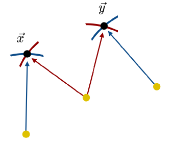
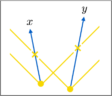
First we summarize the basic strategy to calculate the correlator of the energy-momentum tensor and the resulting GW spectrum. From Eq. (2.43) we see that the spectrum is essentially the unequal-time correlator of the energy-momentum tensor Π(tx,ty,k)Πsubscript𝑡𝑥subscript𝑡𝑦𝑘\Pi(t_{x},t_{y},k), which is the Fourier transform of Π(tx,ty,r)T(tx,x)T(ty,y)similar-toΠsubscript𝑡𝑥subscript𝑡𝑦𝑟delimited-⟨⟩𝑇subscript𝑡𝑥𝑥𝑇subscript𝑡𝑦𝑦\Pi(t_{x},t_{y},\vec{r})\sim\left<T(t_{x},\vec{x})T(t_{y},\vec{y})\right> with T𝑇T symbolically denoting the energy-momentum tensor. Calculating T(tx,x)T(ty,y)delimited-⟨⟩𝑇subscript𝑡𝑥𝑥𝑇subscript𝑡𝑦𝑦\left<T(t_{x},\vec{x})T(t_{y},\vec{y})\right> means

  • Fix the spacetime points x=(tx,x)𝑥subscript𝑡𝑥𝑥x=(t_{x},\vec{x}) and y=(ty,y)𝑦subscript𝑡𝑦𝑦y=(t_{y},\vec{y}).

  • Find those bubble configurations that give nonzero T(x)T(y)𝑇𝑥𝑇𝑦T(x)T(y), estimate the probability for such configurations to occur, and calculate the value of T(x)T(y)𝑇𝑥𝑇𝑦T(x)T(y) in each case.

  • Sum over all such configurations.

As detailed in Appendix A, we may classify the bubble configurations depending on whether the energy-momentum tensor at (tx,x)subscript𝑡𝑥𝑥(t_{x},\vec{x}) and (ty,y)subscript𝑡𝑦𝑦(t_{y},\vec{y}) comes from the same bubble or different bubbles (in other words, the same nucleation point or different nucleation points). We refer to each contribution as

  • Single-bubble,

  • Double-bubble.

Therefore, the resulting GW spectrum ΔΔ\Delta becomes the sum of these two contributions:

ΔΔ\displaystyle\Delta =Δ(s)+Δ(d),absentsuperscriptΔ𝑠superscriptΔ𝑑\displaystyle=\Delta^{(s)}+\Delta^{(d)}, (3.1)

where the superscripts denote “single” and “double,” respectively.♢♢\diamondsuit28♢♢\diamondsuit28\diamondsuit28 The spherical symmetry of a single bubble does not mean that the single-bubble contribution vanishes. See Appendix H on this point.

3.2 Analytic expressions

Now we present the analytic expressions for the GW spectrum. After a short calculation (see Appendix AC), we obtain the single-bubble spectrum

Δ(s)=superscriptΔ𝑠absent\displaystyle\Delta^{(s)}= 𝑑tx𝑑tyv|tx,y|𝑑rtmax𝑑tntntx𝑑txitnty𝑑tyisuperscriptsubscriptdifferential-dsubscript𝑡𝑥superscriptsubscriptdifferential-dsubscript𝑡𝑦superscriptsubscript𝑣subscript𝑡𝑥𝑦differential-d𝑟superscriptsubscriptsubscript𝑡maxdifferential-dsubscript𝑡𝑛superscriptsubscriptsubscript𝑡𝑛subscript𝑡𝑥differential-dsubscript𝑡𝑥𝑖superscriptsubscriptsubscript𝑡𝑛subscript𝑡𝑦differential-dsubscript𝑡𝑦𝑖\displaystyle\int_{-\infty}^{\infty}dt_{x}\int_{-\infty}^{\infty}dt_{y}\int_{v|t_{x,y}|}^{\infty}dr\int_{-\infty}^{t_{\rm max}}dt_{n}\int_{t_{n}}^{t_{x}}dt_{xi}\int_{t_{n}}^{t_{y}}dt_{yi}
k33superscript𝑘33\displaystyle\frac{k^{3}}{3} [eI(xi,yi)Γ(tn)rrxn(s)ryn(s)×[j0(kr)𝒦0(nxn×,nyn×)+j1(kr)kr𝒦1(nxn×,nyn×)+j2(kr)(kr)2𝒦2(nxn×,nyn×)]×txi[rB(txi,tn)3D(tx,txi)]tyi[rB(tyi,tn)3D(ty,tyi)]cos(ktx,y)],\displaystyle\left[\begin{matrix}[l]\displaystyle\;e^{-I(x_{i},y_{i})}\;\Gamma(t_{n})\;\frac{r}{r_{xn}^{(s)}r_{yn}^{(s)}}\\ \displaystyle\times\left[j_{0}(kr){\mathcal{K}}_{0}(n_{xn\times},n_{yn\times})+\frac{j_{1}(kr)}{kr}{\mathcal{K}}_{1}(n_{xn\times},n_{yn\times})+\frac{j_{2}(kr)}{(kr)^{2}}{\mathcal{K}}_{2}(n_{xn\times},n_{yn\times})\right]\\[10.76385pt] \displaystyle\times\;\partial_{txi}\left[r_{B}(t_{xi},t_{n})^{3}D(t_{x},t_{xi})\right]\partial_{tyi}\left[r_{B}(t_{yi},t_{n})^{3}D(t_{y},t_{yi})\right]\cos(kt_{x,y})\end{matrix}\right], (3.2)

and the double-bubble spectrum

Δ(d)=superscriptΔ𝑑absent\displaystyle\Delta^{(d)}= 𝑑tx𝑑tysuperscriptsubscriptdifferential-dsubscript𝑡𝑥superscriptsubscriptdifferential-dsubscript𝑡𝑦\displaystyle\int_{-\infty}^{\infty}dt_{x}\int_{-\infty}^{\infty}dt_{y}
0𝑑rtx𝑑txnty𝑑tyntxntx𝑑txitynty𝑑tyi11𝑑cxn11𝑑cyn02π𝑑ϕxn,ynsuperscriptsubscript0differential-d𝑟superscriptsubscriptsubscript𝑡𝑥differential-dsubscript𝑡𝑥𝑛superscriptsubscriptsubscript𝑡𝑦differential-dsubscript𝑡𝑦𝑛superscriptsubscriptsubscript𝑡𝑥𝑛subscript𝑡𝑥differential-dsubscript𝑡𝑥𝑖superscriptsubscriptsubscript𝑡𝑦𝑛subscript𝑡𝑦differential-dsubscript𝑡𝑦𝑖superscriptsubscript11differential-dsubscript𝑐𝑥𝑛superscriptsubscript11differential-dsubscript𝑐𝑦𝑛superscriptsubscript02𝜋differential-dsubscriptitalic-ϕ𝑥𝑛𝑦𝑛\displaystyle\int_{0}^{\infty}dr\int_{-\infty}^{t_{x}}dt_{xn}\int_{-\infty}^{t_{y}}dt_{yn}\int_{t_{xn}}^{t_{x}}dt_{xi}\int_{t_{yn}}^{t_{y}}dt_{yi}\int_{-1}^{1}dc_{xn}\int_{-1}^{1}dc_{yn}\int_{0}^{2\pi}d\phi_{xn,yn}
k33superscript𝑘33\displaystyle\frac{k^{3}}{3} [Θsp(xi,yn)Θsp(xn,yi)eI(xi,yi)Γ(txn)Γ(tyn)×r2[j0(kr)𝒦0(nxn,nyn)+j1(kr)kr𝒦1(nxn,nyn)+j2(kr)(kr)2𝒦2(nxn,nyn)]×txi[rB(txi,txn)3D(tx,txi)]tyi[rB(tyi,tyn)3D(ty,tyi)]cos(ktx,y)].\displaystyle\left[\begin{matrix}[l]\displaystyle\;\Theta_{\rm sp}(x_{i},y_{n})\Theta_{\rm sp}(x_{n},y_{i})e^{-I(x_{i},y_{i})}\Gamma(t_{xn})\Gamma(t_{yn})\\[4.30554pt] \displaystyle\times\;r^{2}\left[j_{0}(kr){\mathcal{K}}_{0}(n_{xn},n_{yn})+\frac{j_{1}(kr)}{kr}{\mathcal{K}}_{1}(n_{xn},n_{yn})+\frac{j_{2}(kr)}{(kr)^{2}}{\mathcal{K}}_{2}(n_{xn},n_{yn})\right]\\[8.61108pt] \displaystyle\times\;\partial_{txi}\left[r_{B}(t_{xi},t_{xn})^{3}D(t_{x},t_{xi})\right]\partial_{tyi}\left[r_{B}(t_{yi},t_{yn})^{3}D(t_{y},t_{yi})\right]\cos(kt_{x,y})\end{matrix}\right]. (3.3)

Here jnsubscript𝑗𝑛j_{n} are the spherical Bessel functions, and 𝒦nsubscript𝒦𝑛{\mathcal{K}}_{n} functions, expressed by elementary functions, are defined in Appendix F. See Appendix AC for the definition of the other quantities. These expressions apply to a general damping function D𝐷D and a general nucleation rate ΓΓ\Gamma.♢♢\diamondsuit29♢♢\diamondsuit29\diamondsuit29 In Appendix AC we keep the nucleation-time dependence of D𝐷D in order to make the discussion as general as possible. This dependence is omitted in Eqs. (3.2)–(3.3). In addition, though we have derived these expressions by assuming Eqs. (2.16) and (2.21) for the energy-momentum tensor, the derivation is basically the same for other forms.

Given the specific forms for the damping function (2.23) and the nucleation rate (2.24), we can simplify the expressions and obtain Eq. (B.11) for the single-bubble and Eq. (B.20) for the double-bubble, which have now been reduced to five- and nine-dimensional integrations, respectively. For the double-bubble spectrum, we further arrange the expression using a technique detailed in Appendix D to obtain the seven-dimensional integration (D.7).

In Sec. 4 we evaluate the spectrum numerically. However, it is possible to show directly that the spectrum behaves kproportional-toabsent𝑘\propto k for small k𝑘k in the long-lasting limit τ𝜏\tau\to\infty. See the discussion in the latter part of Sec. 5 and Appendix E on this point.

4 Numerical results

In this section we show the results for numerical evaluation of the spectrum (3.2) and (3.3). We show the total spectrum Δ=Δ(s)+Δ(d)ΔsuperscriptΔ𝑠superscriptΔ𝑑\Delta=\Delta^{(s)}+\Delta^{(d)}, changing the duration time of the collided walls τ𝜏\tau. This will tell us how GWs are sourced in time by the bubble dynamics after collisions.

For practical evaluations we use (B.11) and (D.7) for the single- and double-bubble spectrum, respectively. In this section we show the total spectrum Δ=Δ(s)+Δ(d)ΔsuperscriptΔ𝑠superscriptΔ𝑑\Delta=\Delta^{(s)}+\Delta^{(d)} only, and the numerical results for each contribution are shown in Appendix G. Also, all the dimensionful quantities are normalized by β𝛽\beta in the following. In evaluating the spectrum we use a multi-dimensional integration algorithm VEGAS in the CUBA library [95], and cut the calculation at a relative error of 5%percent55\%.

In the present paper we report only for k1less-than-or-similar-to𝑘1k\lesssim 1. This is because for larger k𝑘k the spectrum becomes highly oscillatory and numerical difficulties arise. We leave numerical evaluations for higher wavenumbers as future work.

4.1 Spectral shape

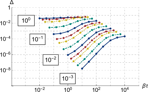
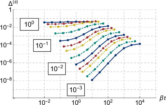
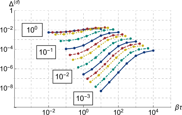
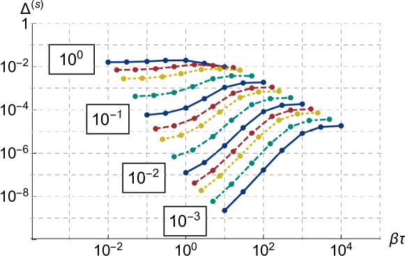
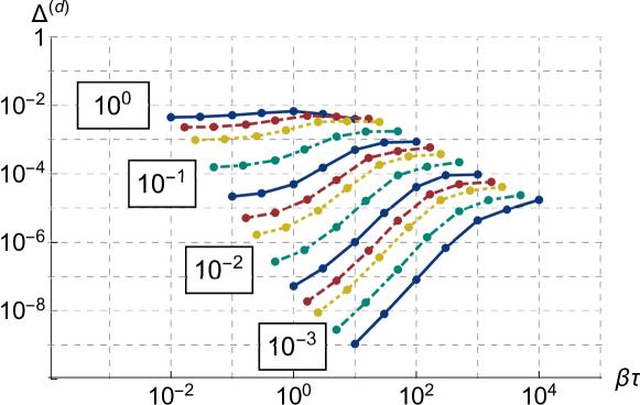
First, we show the spectrum for v=1𝑣1v=1 in Figs. 35. Fig. 3 shows the GW spectrum as a function of the duration time τ𝜏\tau for various wavenumbers from k=0.001𝑘0.001k=0.001 to 111. The blue, red, yellow and green lines denote k=(1,0.6,0.4,0.2)×10n𝑘10.60.40.2superscript10𝑛k=(1,0.6,0.4,0.2)\times 10^{-n} (n)𝑛(n\in\mathbb{Z}), respectively, and these wavenumbers are comparable or smaller than the inverse of the typical bubble size around the time of collisions (which corresponds to k1similar-to𝑘1k\sim 1). The sampling points for the duration time are τ=(0.01,0.03,0.1,0.3,1,3,10)×(1/k)𝜏0.010.030.10.313101𝑘\tau=(0.01,0.03,0.1,0.3,1,3,10)\times(1/k) for each wavenumber. The τ𝜏\tau dependence of the spectrum can be interpreted as denoting the typical sourcing time: for example, if the spectrum grows around τ10similar-to𝜏10\tau\sim 10 for some wavenumber, it means that in the long-lasting limit (τ𝜏\tau\to\infty) the growth typically occurs around time 101010 after the typical collision time. Important features in the spectrum are

  • For a wide range of wavenumbers (smaller than the inverse of the typical bubble size around the time of collisions), the spectrum grows significantly as τ𝜏\tau increases.

  • The growth occurs at τ1/vksimilar-to𝜏1𝑣𝑘\tau\sim 1/vk, and it stops after that.

There is a physical interpretation for the latter: for a fixed wavenumber, GW sourcing occurs when the typical bubble size grows to 1/ksimilar-toabsent1𝑘\sim 1/k. In addition, there is a reason for the termination of the sourcing at late times: see Sec. 5.

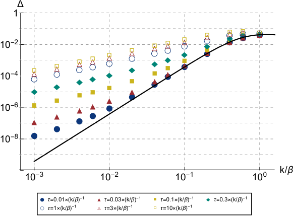
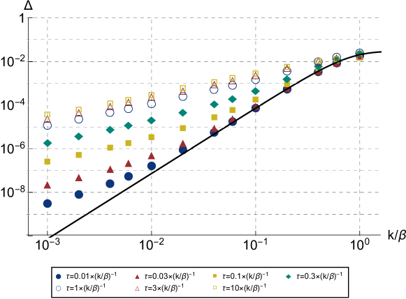
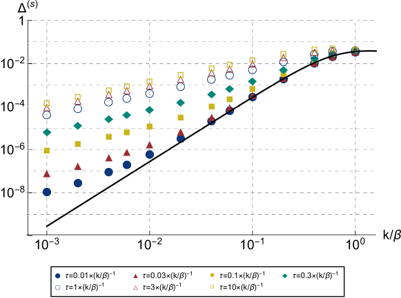
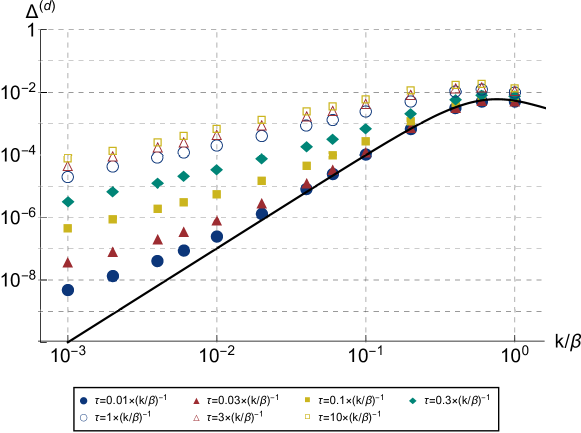
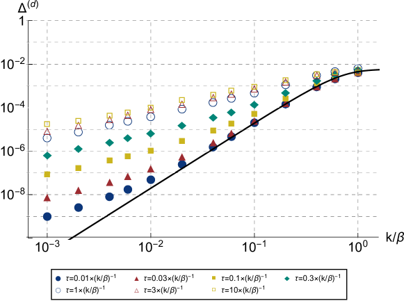
Fig. 4 is essentially the same as Fig. 3, except that the horizontal axis is the wavenumber k𝑘k. Different markers correspond to different values of τ𝜏\tau mentioned above, and the black line is the spectrum with the envelope approximation (instant damping τ=0𝜏0\tau=0) reported in Ref. [85]. It is seen that the spectrum approaches to the black line for small τ𝜏\tau, as expected.♢♢\diamondsuit30♢♢\diamondsuit30\diamondsuit30 For wavenumbers 0.001k0.01less-than-or-similar-to0.001𝑘less-than-or-similar-to0.010.001\lesssim k\lesssim 0.01, we have checked that smaller values for τ𝜏\tau than shown in this plot reproduce the black line. These data are also used in making constant-τ𝜏\tau slices in Fig. 5. An important feature is that

  • The spectrum for low frequencies grows from k3proportional-toabsentsuperscript𝑘3\propto k^{3} to kproportional-toabsent𝑘\propto k,

in the long-lasting limit. There is an explanation for this behavior (see the latter part of Sec. 5) and also an analytic proof on this linear behavior (see Appendix E).

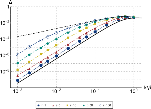
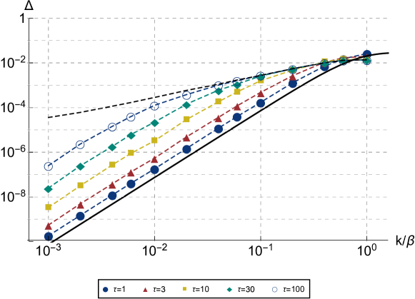
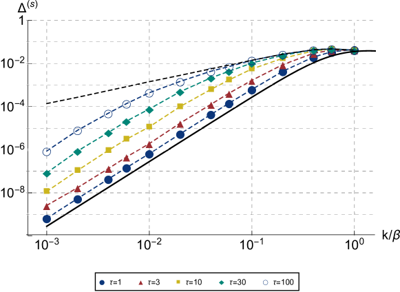
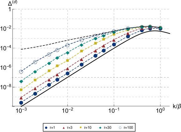
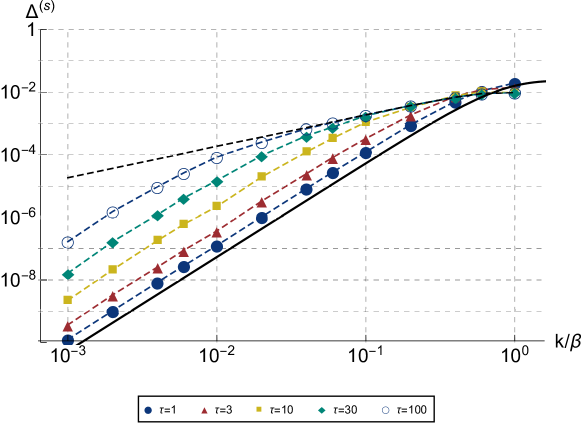
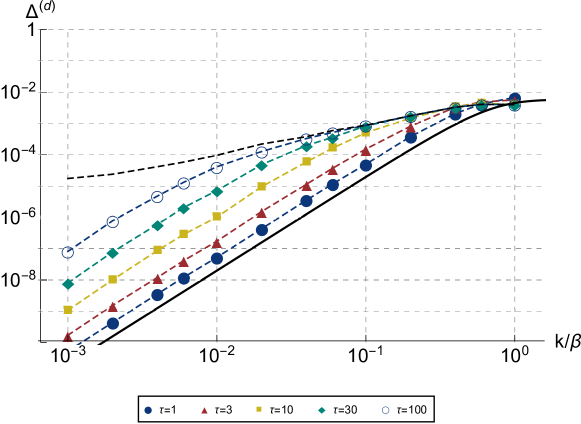
Fig. 5 shows the spectrum at fixed τ𝜏\tau. The colored lines correspond to τ=1,3,10,30,100𝜏131030100\tau=1,3,10,30,100 from bottom to top, while the black-dashed line corresponds to the maximal value of τ𝜏\tau in the data, i.e. τ=10×(1/k)𝜏101𝑘\tau=10\times(1/k). In making this figure we have interpolated the data points shown in Figs. 3 and 4 to make constant-τ𝜏\tau slices. Also, for large wavenumbers k>0.1𝑘0.1k>0.1 we have extrapolated the value at τ=10×(1/k)𝜏101𝑘\tau=10\times(1/k) to larger τ𝜏\tau by assuming that the spectrum is constant for τ>10×(1/k)𝜏101𝑘\tau>10\times(1/k). It is seen that the saturation of the GW spectrum starts from higher wavenumbers as τ𝜏\tau increases.

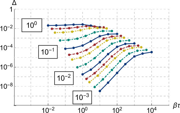
In Figs. 68 we show the spectrum for v=cs𝑣subscript𝑐𝑠v=c_{s}. As discussed in Sec. 2, these figures are considered to be relevant to (b) low terminal velocity. The basic features are the same as Figs. 35.

In Figs. 3 and 6, the low-frequency behavior in the long-lasting limit (black-dashed lines) is approximately given by

ΔΔ\displaystyle\Delta {0.202×(kβ)(v=1),0.0292×(kβ)(v=cs),\displaystyle\simeq\left\{\begin{matrix}0.202\times\displaystyle\left(\frac{k}{\beta}\right)&(v=1),\\[12.91663pt] 0.0292\times\displaystyle\left(\frac{k}{\beta}\right)&(v=c_{s}),\end{matrix}\right. (4.1)

for k/β1less-than-or-similar-to𝑘𝛽1k/\beta\lesssim 1.♢♢\diamondsuit31♢♢\diamondsuit31\diamondsuit31 For k/βH/βless-than-or-similar-to𝑘𝛽𝐻𝛽k/\beta\lesssim H/\beta the cosmic expansion will no longer be negligible, and the spectrum is expected to be suppressed.

4.2 Peak position

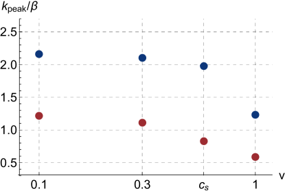
In Fig. 9 we show the peak wavenumber of the spectrum with the envelope approximation (blue) and without the envelope approximation (red). In calculating the latter we have used the data for τ=10×(1/k)𝜏101𝑘\tau=10\times(1/k), assuming that the spectrum is constant for larger values of τ𝜏\tau. It is seen that the peak position moves to lower k𝑘k in the long-lasting limit.


Refer to caption
Figure 3: The total spectrum ΔΔ\Delta as a function of the duration time τ𝜏\tau for v=1𝑣1v=1. The blue, red, yellow and green lines correspond to k=(1,0.6,0.4,0.2)×10n𝑘10.60.40.2superscript10𝑛k=(1,0.6,0.4,0.2)\times 10^{-n} (n𝑛n\in\mathbb{Z}), respectively.
Refer to caption
Figure 4: The total spectrum ΔΔ\Delta as a function of wavenumber k𝑘k for v=1𝑣1v=1. Each data point corresponds to τ=(0.01,0.03,0.1,0.3,1,3,10)×(1/k)𝜏0.010.030.10.313101𝑘\tau=(0.01,0.03,0.1,0.3,1,3,10)\times(1/k), while the black line shows the spectrum with the envelope approximation obtained in Ref. [85].
Refer to caption
Figure 5: The total spectrum ΔΔ\Delta as a function of wavenumber k𝑘k for v=1𝑣1v=1. Each colored line corresponds to τ=1,3,10,30,100𝜏131030100\tau=1,3,10,30,100 from bottom to top, while the black-dashed line corresponds to the data points for τ=10×(1/k)𝜏101𝑘\tau=10\times(1/k). The black-solid line is the same as Fig. 4.
Refer to caption
Figure 6: Same as Fig. 3 except that v=cs𝑣subscript𝑐𝑠v=c_{s}.
Refer to caption
Figure 7: Same as Fig. 4 except that v=cs𝑣subscript𝑐𝑠v=c_{s}.
Refer to caption
Figure 8: Same as Fig. 5 except that v=cs𝑣subscript𝑐𝑠v=c_{s}.
Refer to caption
Figure 9: Peak position of the spectrum with the envelope approximation (blue) and without the envelope approximation (red).

5 Discussion and conclusions

In this paper we have studied GW production from bubble dynamics in cosmic first-order phase transitions. We have used the method of relating the GW spectrum with the two-point correlator of the energy-momentum tensor T(x)T(y)delimited-⟨⟩𝑇𝑥𝑇𝑦\left<T(x)T(y)\right> by using the stochasticity of produced GWs. In calculating the correlator, the main approximations we have adopted in this paper are

  • (1)

    Exponential form for the nucleation rate (Eq. (2.24)),

  • (2)

    Thin-wall approximation (Eqs. (2.16) and (2.21)),

  • (3)

    Free propagation after bubble collisions (Eqs. (2.16) and (2.21)),

and thus we have generalized our previous result [85] by removing the envelope approximation. As explained in Sec. 2, the approximations we adopt in this paper are expected to give a reasonable modeling of the system for frequencies around or lower than the inverse of the typical bubble size around the time of collisions, as long as the phase transition proceeds with either (a) runaway or (b) low terminal velocity.♢♢\diamondsuit32♢♢\diamondsuit32\diamondsuit32 In Ref. [73] it has been reported that the peak of the spectrum is located at frequencies around the inverse of the bubble wall width. In fact, bubble wall width seems to be one of the characteristic scales in cosmological first-order phase transitions. However, our current formalism cannot take such a finite wall width into account, which will affect the spectrum at frequencies higher than the inverse of the bubble radius around the time of collisions. It would be one of the future directions to consider how to deal with the finite wall width in the present formalism. The remaining case, (c) high terminal velocity, would require the analysis of nonlinear dynamics, and beyond the scope of this paper.

Our main results are the analytic expressions in Sec. 3 (Eqs. (3.2) and (3.3)), and the numerical results presented in Sec. 4:

  • For the analytic expressions, they apply to a general damping function D𝐷D (see Sec. 2.2) and a general nucleation rate ΓΓ\Gamma (see Sec. 2.3). Also, it can be shown that the spectrum behaves as kproportional-toabsent𝑘\propto k for small k𝑘k in the long-lasting limit of bubble walls (see the discussion below and also Appendix E).

  • In Sec. 4, we have performed numerical evaluation of the spectrum obtained in Sec. 3. It is found that the spectrum shows a significant enhancement in the long-lasting limit of bubble walls, compared to the one with the envelope approximation. It is also found that the spectrum growth occurs as a transition from k3proportional-toabsentsuperscript𝑘3\propto k^{3} to kproportional-toabsent𝑘\propto k for small wavenumbers. For a fixed wavenumber k𝑘k, such a transition typically occurs time 1/vksimilar-toabsent1𝑣𝑘\sim 1/vk after collision, which has a physical interpretation that the sourcing occurs when the (collided) bubbles expand to size 1/ksimilar-toabsent1𝑘\sim 1/k. Also, the sourcing terminates after this typical sourcing time.

At this point we compare our results with the literature. The results we have obtained in Sec. 4 and the ones in the numerical simulation literature seems to have some discrepancies. It is commonly considered that GW sourcing from sound waves continues all the way until the Hubble time after bubble collisions because of the long-lasting nature of the source. This argument is based on the following ansatz on the correlator ΠΠ\Pi at late times:

Π(tx,ty,k)Πsubscript𝑡𝑥subscript𝑡𝑦𝑘\displaystyle\Pi(t_{x},t_{y},k) =?Π(txty,k).?Πsubscript𝑡𝑥subscript𝑡𝑦𝑘\displaystyle\overset{?}{=}\Pi(t_{x}-t_{y},k). (5.1)

However, if this argument holds true, the GW spectrum presented in this paper would show a linear enhancement in the duration time of the bubble walls τ𝜏\tau, as long as our modeling of the system correctly captures the dynamics at least for low frequencies (i.e. frequencies lower than the inverse of the typical bubble size around the time of collisions). Instead, what we have observed is the termination of the sourcing and the resulting saturation of the spectrum in the long-lasting limit. Within the modeling of the system we have presented in this paper, there is a clear reason why Eq. (5.1) does not hold at least for low frequencies:

  • GWs are sourced by the two-point correlator of the energy-momentum tensor T(x)T(y)delimited-⟨⟩𝑇𝑥𝑇𝑦\left<T(x)T(y)\right>, or more precisely, the projected correlator KKT(x)T(y)𝐾𝐾delimited-⟨⟩𝑇𝑥𝑇𝑦KK\left<T(x)T(y)\right> (see Sec. 2.4). On the other hand, the projected one-point correlator KT(x)𝐾delimited-⟨⟩𝑇𝑥K\left<T(x)\right> vanishes because of the spherical symmetry of the system makes T(x)δijproportional-todelimited-⟨⟩𝑇𝑥subscript𝛿𝑖𝑗\left<T(x)\right>\propto\delta_{ij}.

  • Therefore, in order to produce nonzero KKT(x)T(y)𝐾𝐾delimited-⟨⟩𝑇𝑥𝑇𝑦KK\left<T(x)T(y)\right>, the contribution to the energy-momentum tensor at the spacetime point x𝑥x must affect the energy-momentum tensor at y𝑦y in some way. Taking into account the fact that bubble nucleation finishes within the timescale of 1/βsimilar-toabsent1𝛽\sim 1/\beta, this means that the bubble which affects T(x)𝑇𝑥T(x) and the one which affects T(y)𝑇𝑦T(y) must nucleate within a distance of 𝒪(1/β)similar-toabsent𝒪1𝛽\sim{\mathcal{O}}(1/\beta)♢♢\diamondsuit33♢♢\diamondsuit33\diamondsuit33 In the single-bubble case this is automatically satisfied because the two bubbles are identical, while in the double-bubble case the two bubbles give a net contribution to KKT(x)T(y)𝐾𝐾delimited-⟨⟩𝑇𝑥𝑇𝑦KK\left<T(x)T(y)\right> only when the nucleation points are close with each other 𝒪(1/β)similar-toabsent𝒪1𝛽\sim{\mathcal{O}}(1/\beta). (Fig. 26 might be of some help).

  • Let us see this from a different viewpoint. In the system under consideration, we may divide the bubbles into some groups in which the nucleation points are within a radius of 𝒪(1/β)similar-toabsent𝒪1𝛽\sim{\mathcal{O}}(1/\beta), which we call “correlation groups” (see Fig. 10). These correlation groups just expand as time goes without affecting each other. Gravitational-wave production in this system can be modeled just by the sum of sourcing from these independent sources, because they have only suppressed correlations with each other even after they overlap. In this modeling, GW sourcing at wavenumber k𝑘k occurs only when the correlation groups expand to a size 1/ksimilar-toabsent1𝑘\sim 1/k, and there is no sourcing at later times.

  • In addition, one can show that this modeling reproduces the observed behavior of the spectrum Δkproportional-toΔ𝑘\Delta\propto k for low frequencies. First note that

    • Relativistic objects with energy density ρsourcesubscript𝜌source\rho_{\rm source} and size 1/ksimilar-toabsent1𝑘\sim 1/k which last for a period ΔtΔ𝑡\Delta t produces GWs with a typical amplitude ΩGW(ρtot/MP2)(ρsource/ρtot)2(Δt)2similar-tosubscriptΩGWsubscript𝜌totsuperscriptsubscript𝑀𝑃2superscriptsubscript𝜌sourcesubscript𝜌tot2superscriptΔ𝑡2\Omega_{\rm GW}\sim(\rho_{\rm tot}/M_{P}^{2})(\rho_{\rm source}/\rho_{\rm tot})^{2}(\Delta t)^{2} at wavenumber k𝑘k.♢♢\diamondsuit34♢♢\diamondsuit34\diamondsuit34 This can be derived for example from the equation of motion as h\displaystyle\Box h ρsourceMP2ρGWρsource2Δt2MP2ΩGWρtotMP2ρsource2ρtot2Δt2.formulae-sequencesimilar-toabsentsubscript𝜌sourcesuperscriptsubscript𝑀𝑃2formulae-sequencesimilar-tosubscript𝜌GWsuperscriptsubscript𝜌source2Δsuperscript𝑡2superscriptsubscript𝑀𝑃2similar-tosubscriptΩGWsubscript𝜌totsuperscriptsubscript𝑀𝑃2superscriptsubscript𝜌source2superscriptsubscript𝜌tot2Δsuperscript𝑡2\displaystyle\sim\frac{\rho_{\rm source}}{M_{P}^{2}}\;\;\;\;\to\;\;\;\;\rho_{\rm GW}\sim\frac{\rho_{\rm source}^{2}\Delta t^{2}}{M_{P}^{2}}\;\;\;\;\to\;\;\;\;\Omega_{\rm GW}\sim\frac{\rho_{\rm tot}}{M_{P}^{2}}\frac{\rho_{\rm source}^{2}}{\rho_{\rm tot}^{2}}\Delta t^{2}. (5.2) Also, with ρsourceκρ0similar-tosubscript𝜌source𝜅subscript𝜌0\rho_{\rm source}\sim\kappa\rho_{0}, this reproduces the well-known behavior of GWs from bubble collisions ΩGWκ2(Hβ)2(α1+α)2.similar-tosubscriptΩGWsuperscript𝜅2superscriptsubscript𝐻𝛽2superscript𝛼1𝛼2\displaystyle\Omega_{\rm GW}\sim\kappa^{2}\left(\frac{H_{*}}{\beta}\right)^{2}\left(\frac{\alpha}{1+\alpha}\right)^{2}. (5.3)

    Then also note that in the present setup there are (k/β)3similar-toabsentsuperscript𝑘𝛽3\sim(k/\beta)^{-3} overlapping independent sources at time 1/ksimilar-toabsent1𝑘\sim 1/k after collisions. Each source has energy density ρsourcek3proportional-tosubscript𝜌sourcesuperscript𝑘3\rho_{\rm source}\propto k^{3} and lasts for Δt1/ksimilar-toΔ𝑡1𝑘\Delta t\sim 1/k. Therefore one finds ΩGWk3(k3)2(k1)2kproportional-tosubscriptΩGWsuperscript𝑘3superscriptsuperscript𝑘32superscriptsuperscript𝑘12proportional-to𝑘\Omega_{\rm GW}\propto k^{-3}\cdot(k^{3})^{2}\cdot(k^{-1})^{2}\propto k,♢♢\diamondsuit35♢♢\diamondsuit35\diamondsuit35 More precisely, from ρsource(k/β)3κρ0similar-tosubscript𝜌sourcesuperscript𝑘𝛽3𝜅subscript𝜌0\rho_{\rm source}\sim(k/\beta)^{3}\kappa\rho_{0}, the GW spectrum becomes ΩGW(βk)3ρtotMP2((k/β)3κρ0ρtot)2(1k)2(kβ)κ2(Hβ)2(α1+α)2,similar-tosubscriptΩGWsuperscript𝛽𝑘3subscript𝜌totsuperscriptsubscript𝑀𝑃2superscriptsuperscript𝑘𝛽3𝜅subscript𝜌0subscript𝜌tot2superscript1𝑘2similar-to𝑘𝛽superscript𝜅2superscriptsubscript𝐻𝛽2superscript𝛼1𝛼2\displaystyle\Omega_{\rm GW}\sim\left(\frac{\beta}{k}\right)^{3}\cdot\frac{\rho_{\rm tot}}{M_{P}^{2}}\left(\frac{(k/\beta)^{3}\kappa\rho_{0}}{\rho_{\rm tot}}\right)^{2}\left(\frac{1}{k}\right)^{2}\sim\left(\frac{k}{\beta}\right)\cdot\kappa^{2}\left(\frac{H_{*}}{\beta}\right)^{2}\left(\frac{\alpha}{1+\alpha}\right)^{2}, (5.4) at low frequencies kβless-than-or-similar-to𝑘𝛽k\lesssim\beta. and hence our modeling of the system by independent expanding sources captures the late time GW sourcing quite well.

At the current stage we do not have any argument which reconciles above reasoning with the sound-wave enhancement of GWs in the literature.

Finally we discuss the effect of finite wall width in the low terminal velocity case. As mentioned in Sec. 2.1 (b), the region of energy concentration increases in volume after bubble collisions. Such wall regions eventually fill the whole Universe and start to overlap with each other.♢♢\diamondsuit36♢♢\diamondsuit36\diamondsuit36 Note that, as mentioned in Sec. 2.1 (b), the width of such wall regions remains to be constant while their area increases as bubbles expand. One might worry that the description of the present system by the thin-wall approximation would not be valid any longer after such overlaps start to develop. However, these overlaps do not necessarily mean the breakdown of the thin-wall approximation. This is because most overlaps are supposed to be irrelevant in GW production: as we have just seen, two bubbles with nucleation points more than 𝒪(1/β)𝒪1𝛽{\mathcal{O}}(1/\beta) distant from each other have only suppressed correlation, and their overlap is quite unlikely to affect GW production. In this sense, we only have to focus on each correlation group in discussing GW production. For each group the volume fraction of the wall regions does not increase even well after collisions (see Fig. 10). Therefore, the thin-wall approximation is still expected to be a good description of the system for GW frequencies lower than the inverse of the wall width.

Though much remains to be settled, the analytic approach to the dynamics of GW sourcing in first-order phase transitions as we have presented in this paper will work complementarily with numerical simulations. We believe that such a direction is worth further investigation in the future.
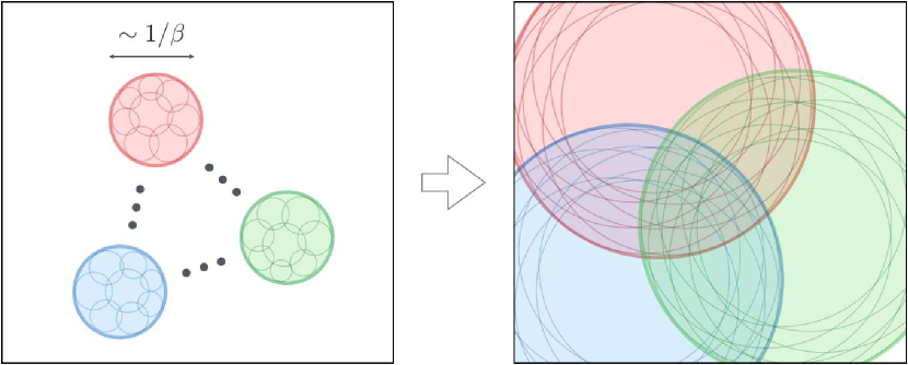
Refer to caption
Figure 10: Schematic picture of the “correlation groups.” Bubbles are divided into groups which typically have radius 1/βsimilar-toabsent1𝛽\sim 1/\beta around the time of phase transition (left). These bubbles have correlation with each other only within each group, and correlation across different groups are (exponentially) suppressed. As long as free propagation after bubble collisions makes a good approximation of the system, these groups have no correlation even after they expand and overlap with each other, and can be regarded as independent sources of GWs (right).

Acknowledgments

R.J. is grateful to M. Hindmarsh, S. Huber, T. Konstandin and J. M. No for helpful discussions. The work of R.J. was supported by IBS under the project code, IBS-R018-D1. The work of R.J. and M.T. was supported by JSPS Research Fellowships for Young Scientists.

Appendix A GW spectrum with the envelope approximation

In this appendix we derive the GW spectrum by evaluating the unequal-time power spectrum Π(tx,ty,k)Πsubscript𝑡𝑥subscript𝑡𝑦𝑘\Pi(t_{x},t_{y},k), or equivalently the correlator T(x)T(y)delimited-⟨⟩𝑇𝑥𝑇𝑦\langle T(x)T(y)\rangle. Though our main goal is to derive it without the envelope approximation, we first illustrate the calculation procedure with this approximation. This is because the full derivation of the correlator in Sec. B is somewhat complicated, and therefore it would be better to see a simpler example first. We use Eq. (2.16)–(2.19) for the energy-momentum tensor of uncollided bubble walls, while we assume that it vanishes instantly after collision. This appendix basically follows Ref. [85].

A.1 Basic strategy

We first explain the essence for the derivation of the GW spectrum. From the definition of the ensemble average, all we have to do to obtain T(x)T(y)delimited-⟨⟩𝑇𝑥𝑇𝑦\langle T(x)T(y)\rangle is

  • Fix the spacetime points x=(tx,x)𝑥subscript𝑡𝑥𝑥x=(t_{x},\vec{x}) and y=(ty,y)𝑦subscript𝑡𝑦𝑦y=(t_{y},\vec{y}).

  • Find bubble configurations giving nonzero T(x)T(y)𝑇𝑥𝑇𝑦T(x)T(y), estimate the probability for such configurations to occur, and calculate the value of T(x)T(y)𝑇𝑥𝑇𝑦T(x)T(y) in each case.

  • Sum over all possible configurations.

We call x𝑥x and y𝑦y in the arguments of T(x)T(y)delimited-⟨⟩𝑇𝑥𝑇𝑦\langle T(x)T(y)\rangle “(spacetime) evaluation point” in the following. Also, txsubscript𝑡𝑥t_{x} and tysubscript𝑡𝑦t_{y} are called “evaluation time”, while x𝑥\vec{x} and y𝑦\vec{y} are called “(spacial) evaluation point”.

Let us consider which bubble configurations give nonzero T(x)T(y)𝑇𝑥𝑇𝑦T(x)T(y). In order for this to occur, some bubble wall fragment(s) must be at x𝑥\vec{x} at time txsubscript𝑡𝑥t_{x}, and other(s) must be at y𝑦\vec{y} at time tysubscript𝑡𝑦t_{y}♢♢\diamondsuit37♢♢\diamondsuit37\diamondsuit37 If one takes radiation component and the false-vacuum energy into account, the energy-momentum tensor is nonzero even when there is no bubble wall at x𝑥x or y𝑦y. However, these contributions are isotropic and they vanish after multiplied to the projection operator (2.28). . We refer to such bubbles whose wall pass through x𝑥\vec{x} at txsubscript𝑡𝑥t_{x} or y𝑦\vec{y} at tysubscript𝑡𝑦t_{y} as x𝑥x-bubble or y𝑦y-bubble, respectively, and call the wall fragments which pass these spacetime evaluation points x𝑥x-fragment or y𝑦y-fragment, respectively. See Fig. 11 for illustration. In this figure, bubble nucleation points are denoted by the yellow circles. The red bubble is x𝑥x-bubble and y𝑦y-bubble (which we call xy𝑥𝑦xy-bubble), while the left and right blue ones are x𝑥x-bubble and y𝑦y-bubble, respectively.

Next we take the thin-wall limit lB0subscript𝑙𝐵0l_{B}\to 0 into account. In this limit we do not have to consider those cases where two different fragments exist at a single spacetime evaluation point, because such a probability is infinitely smaller than the probability for one fragment to exist at the point. Therefore we consider one wall fragment at x𝑥x, and another at y𝑦y. There are two possibilities for this: one is that these fragments originate from the same nucleation point (red lines in Fig. 11), while the other is that these come from different nucleation points (blue lines in Fig. 11). This leads to the following classification:♢♢\diamondsuit38♢♢\diamondsuit38\diamondsuit38 One may wonder why the single-bubble contribution has to be taken into account, because it is well known that a spherical object does not radiate GWs. The answer is that fixing the spacetime points x𝑥x and y𝑦y breaks the spherical symmetry of a single bubble. See Appendix H on this point.

  • Single-bubble:
    The wall fragments passing through x𝑥x and y𝑦y originate from a single nucleation point.

  • Double-bubble:
    The wall fragments passing through x𝑥x and y𝑦y originate from two different nucleation points.

In the rest of this appendix we calculate these contributions in turn, using the envelope approximation mentioned in Sec. 1 and Sec. 2.2. The final expressions are shown in Eqs. (A.23) and (A.31) for single- and double-bubble contributions, respectively.

Before going into calculation of the spectrum, we first fix our notations and then introduce the “false vacuum probability”. These are repeatedly used in the following calculations. Also we take β=1𝛽1\beta=1 unit without loss of generality.

Refer to caption
Figure 11: Rough sketch of the single- and double-bubble contributions. In single-bubble contribution (red), the bubble wall fragments passing through x𝑥\vec{x} and y𝑦\vec{y} come from the single nucleation point, while in double-bubble contribution (blue) they belong to different nucleation points. In this figure the evaluation times are taken to be tx=tysubscript𝑡𝑥subscript𝑡𝑦t_{x}=t_{y} for illustrative purpose.

A.2 Prerequisites

Notations

In this subsection we fix our notations and conventions. We denote the two spacetime points in the correlator as (see Fig. 12)

x𝑥\displaystyle x =(tx,x),y=(ty,y),formulae-sequenceabsentsubscript𝑡𝑥𝑥𝑦subscript𝑡𝑦𝑦\displaystyle=(t_{x},\vec{x}),\;\;\;y=(t_{y},\vec{y}), (A.1)

and write the average and difference of the time coordinates as

tx,ysubscript𝑡𝑥𝑦\displaystyle t_{\langle x,y\rangle} tx+ty2,tx,ytxty.formulae-sequenceabsentsubscript𝑡𝑥subscript𝑡𝑦2subscript𝑡𝑥𝑦subscript𝑡𝑥subscript𝑡𝑦\displaystyle\equiv\frac{t_{x}+t_{y}}{2},\;\;\;t_{x,y}\equiv t_{x}-t_{y}. (A.2)

We sometimes use these quantities in place of txsubscript𝑡𝑥t_{x} and tysubscript𝑡𝑦t_{y}. Also, the distance between x𝑥\vec{x} and y𝑦\vec{y} is denoted by

rxy,r𝑟𝑥𝑦𝑟\displaystyle\vec{r}\equiv\vec{x}-\vec{y},\;\;\;r |r|.absent𝑟\displaystyle\equiv|\vec{r}|. (A.3)

For later convenience, we define the spacial distance normalized by the wall velocity v𝑣v:

rvsubscript𝑟𝑣\displaystyle r_{v} rv.absent𝑟𝑣\displaystyle\equiv\frac{r}{v}. (A.4)

In what follows we often consider past cones with velocity v𝑣v originating from x𝑥x and y𝑦y (see Fig. 12 and 13), and we refer to these as past v𝑣v-cones. These coincide with past light cones for luminal wall case v=1𝑣1v=1. We label these by Sxsubscript𝑆𝑥S_{x} and Sysubscript𝑆𝑦S_{y}. The regions inside Sxsubscript𝑆𝑥S_{x} and Sysubscript𝑆𝑦S_{y} are called Vxsubscript𝑉𝑥V_{x} and Vysubscript𝑉𝑦V_{y}, respectively, and their union is written as VxyVxVysubscript𝑉𝑥𝑦subscript𝑉𝑥subscript𝑉𝑦V_{xy}\equiv V_{x}\cup V_{y}. Also, we define the following spacetime points

x+δ𝑥𝛿\displaystyle x+\delta (tx+lB/v,x),y+δ(ty+lB/v,y).formulae-sequenceabsentsubscript𝑡𝑥subscript𝑙𝐵𝑣𝑥𝑦𝛿subscript𝑡𝑦subscript𝑙𝐵𝑣𝑦\displaystyle\equiv(t_{x}+l_{B}/v,\vec{x}),\;\;\;y+\delta\equiv(t_{y}+l_{B}/v,\vec{y}). (A.5)

We denote their past v𝑣v-cones by Sx+δsubscript𝑆𝑥𝛿S_{x+\delta} and Sy+δsubscript𝑆𝑦𝛿S_{y+\delta}, and their inner regions by Vx+δsubscript𝑉𝑥𝛿V_{x+\delta} and Vy+δsubscript𝑉𝑦𝛿V_{y+\delta}. The thin regions on the surface of Vxsubscript𝑉𝑥V_{x} and Vysubscript𝑉𝑦V_{y} with width lB/vsubscript𝑙𝐵𝑣l_{B}/v are written as

δVx𝛿subscript𝑉𝑥\displaystyle\delta V_{x} Vx+δVx,δVyVy+δVy.formulae-sequenceabsentsubscript𝑉𝑥𝛿subscript𝑉𝑥𝛿subscript𝑉𝑦subscript𝑉𝑦𝛿subscript𝑉𝑦\displaystyle\equiv V_{x+\delta}-V_{x},\;\;\;\delta V_{y}\equiv V_{y+\delta}-V_{y}. (A.6)

The intersection of these regions is denoted by

δVxy𝛿subscript𝑉𝑥𝑦\displaystyle\delta V_{xy} δVxδVy.absent𝛿subscript𝑉𝑥𝛿subscript𝑉𝑦\displaystyle\equiv\delta V_{x}\cap\delta V_{y}. (A.7)

We also define the following region for later use

δVx(y)𝛿superscriptsubscript𝑉𝑥𝑦\displaystyle\delta V_{x}^{(y)} δVxVy+δ,δVy(x)δVyVx+δ.formulae-sequenceabsent𝛿subscript𝑉𝑥subscript𝑉𝑦𝛿𝛿superscriptsubscript𝑉𝑦𝑥𝛿subscript𝑉𝑦subscript𝑉𝑥𝛿\displaystyle\equiv\delta V_{x}-V_{y+\delta},\;\;\;\delta V_{y}^{(x)}\equiv\delta V_{y}-V_{x+\delta}. (A.8)

Fig. 12 summarizes these notations.

Next, let us consider a constant-time hypersurface ΣtsubscriptΣ𝑡\Sigma_{t} at time t𝑡t. The two past v𝑣v-cones Sxsubscript𝑆𝑥S_{x} and Sysubscript𝑆𝑦S_{y} form spheres on this hypersurface as shown in Fig. 14. We call these two spheres Cxsubscript𝐶𝑥C_{x} and Cysubscript𝐶𝑦C_{y}, and call their centers Oxsubscript𝑂𝑥O_{x} and Oysubscript𝑂𝑦O_{y}. The radii of Cxsubscript𝐶𝑥C_{x} and Cysubscript𝐶𝑦C_{y} are given by

rxsubscript𝑟𝑥\displaystyle r_{x} rB(tx,t),ryrB(ty,t),formulae-sequenceabsentsubscript𝑟𝐵subscript𝑡𝑥𝑡subscript𝑟𝑦subscript𝑟𝐵subscript𝑡𝑦𝑡\displaystyle\equiv r_{B}(t_{x},t),\;\;\;\;r_{y}\equiv r_{B}(t_{y},t), (A.9)

respectively. These spheres Cxsubscript𝐶𝑥C_{x} and Cysubscript𝐶𝑦C_{y} have intersection only for t<tmax𝑡subscript𝑡maxt<t_{\rm max} with

tmaxsubscript𝑡max\displaystyle t_{\rm max} tx+tyrv2.absentsubscript𝑡𝑥subscript𝑡𝑦subscript𝑟𝑣2\displaystyle\equiv\frac{t_{x}+t_{y}-r_{v}}{2}. (A.10)

Let Pxsubscript𝑃𝑥P_{x} and Pysubscript𝑃𝑦P_{y} be some arbitrary points on Cxsubscript𝐶𝑥C_{x} and Cysubscript𝐶𝑦C_{y}. These points are parametrized by nxOxPx/|OxPx|subscript𝑛𝑥subscript𝑂𝑥subscript𝑃𝑥subscript𝑂𝑥subscript𝑃𝑥n_{x}\equiv\overrightarrow{O_{x}P_{x}}/|\overrightarrow{O_{x}P_{x}}| and nyOyPy/|OyPy|subscript𝑛𝑦subscript𝑂𝑦subscript𝑃𝑦subscript𝑂𝑦subscript𝑃𝑦n_{y}\equiv\overrightarrow{O_{y}P_{y}}/|\overrightarrow{O_{y}P_{y}}|. We parametrize these unit vectors so that θxsubscript𝜃𝑥\theta_{x} and θysubscript𝜃𝑦\theta_{y} denote the polar angle and ϕxsubscriptitalic-ϕ𝑥\phi_{x} and ϕysubscriptitalic-ϕ𝑦\phi_{y} denote the azimuthal angle with respect to r𝑟\vec{r}:

nxsubscript𝑛𝑥\displaystyle n_{x} (sxcϕx,sxsϕx,cx),ny(sycϕy,sysϕy,cy),formulae-sequenceabsentsubscript𝑠𝑥subscript𝑐italic-ϕ𝑥subscript𝑠𝑥subscript𝑠italic-ϕ𝑥subscript𝑐𝑥subscript𝑛𝑦subscript𝑠𝑦subscript𝑐italic-ϕ𝑦subscript𝑠𝑦subscript𝑠italic-ϕ𝑦subscript𝑐𝑦\displaystyle\equiv(s_{x}c_{\phi x},s_{x}s_{\phi x},c_{x}),\;\;\;n_{y}\equiv(s_{y}c_{\phi y},s_{y}s_{\phi y},c_{y}), (A.11)

and often write cosθx(θy)subscript𝜃𝑥subscript𝜃𝑦\cos\theta_{x}(\theta_{y}) and sinθx(θy)subscript𝜃𝑥subscript𝜃𝑦\sin\theta_{x}(\theta_{y}) as cx(cy)subscript𝑐𝑥subscript𝑐𝑦c_{x}(c_{y}) and sx(sy)subscript𝑠𝑥subscript𝑠𝑦s_{x}(s_{y}), respectively, and cosϕx(ϕy)subscriptitalic-ϕ𝑥subscriptitalic-ϕ𝑦\cos\phi_{x}(\phi_{y}) and sinϕx(ϕy)subscriptitalic-ϕ𝑥subscriptitalic-ϕ𝑦\sin\phi_{x}(\phi_{y}) as cϕx(cϕy)subscript𝑐italic-ϕ𝑥subscript𝑐italic-ϕ𝑦c_{\phi x}(c_{\phi y}) and sϕx(sϕy)subscript𝑠italic-ϕ𝑥subscript𝑠italic-ϕ𝑦s_{\phi x}(s_{\phi y}), respectively. We also define the following product N𝑁N of the unit vectors for later convenience:

Nijklsubscript𝑁𝑖𝑗𝑘𝑙\displaystyle N_{ijkl} (nx)i(nx)j(ny)k(ny)l.absentsubscriptsubscript𝑛𝑥𝑖subscriptsubscript𝑛𝑥𝑗subscriptsubscript𝑛𝑦𝑘subscriptsubscript𝑛𝑦𝑙\displaystyle\equiv(n_{x})_{i}(n_{x})_{j}(n_{y})_{k}(n_{y})_{l}. (A.12)

In addition, we often consider those cases where Pxsubscript𝑃𝑥P_{x} and Pysubscript𝑃𝑦P_{y} are identical (i.e. they are an identical point on the intersection of Cxsubscript𝐶𝑥C_{x} and Cysubscript𝐶𝑦C_{y}). In such cases we write Px=Py=Psubscript𝑃𝑥subscript𝑃𝑦𝑃P_{x}=P_{y}=P, and label the quantities introduced above by “×\times”: nxsubscript𝑛𝑥n_{x} and nysubscript𝑛𝑦n_{y} as nx×subscript𝑛𝑥n_{x\times} and ny×subscript𝑛𝑦n_{y\times}, θxsubscript𝜃𝑥\theta_{x} and θysubscript𝜃𝑦\theta_{y} as θx×subscript𝜃𝑥\theta_{x\times} and θy×subscript𝜃𝑦\theta_{y\times}, and ϕxsubscriptitalic-ϕ𝑥\phi_{x} and ϕysubscriptitalic-ϕ𝑦\phi_{y} as ϕ×subscriptitalic-ϕ\phi_{\times}, respectively. In such cases, the cosines of the polar angles are related with the radii of Cxsubscript𝐶𝑥C_{x} and Cysubscript𝐶𝑦C_{y} as

cosθx×subscript𝜃𝑥\displaystyle\cos\theta_{x\times} =r2+rx2ry22rrx,cosθy×=r2+ry2rx22rry.formulae-sequenceabsentsuperscript𝑟2superscriptsubscript𝑟𝑥2superscriptsubscript𝑟𝑦22𝑟subscript𝑟𝑥subscript𝜃𝑦superscript𝑟2superscriptsubscript𝑟𝑦2superscriptsubscript𝑟𝑥22𝑟subscript𝑟𝑦\displaystyle=-\frac{r^{2}+r_{x}^{2}-r_{y}^{2}}{2rr_{x}},\;\;\;\;\cos\theta_{y\times}=\frac{r^{2}+r_{y}^{2}-r_{x}^{2}}{2rr_{y}}. (A.13)

Likewise, the product of the unit vectors N𝑁N is written as N×subscript𝑁N_{\times}:

N×,ijklsubscript𝑁𝑖𝑗𝑘𝑙\displaystyle N_{\times,ijkl} =(nx×)i(nx×)j(ny×)k(ny×)l.absentsubscriptsubscript𝑛𝑥𝑖subscriptsubscript𝑛𝑥𝑗subscriptsubscript𝑛𝑦𝑘subscriptsubscript𝑛𝑦𝑙\displaystyle=(n_{x\times})_{i}(n_{x\times})_{j}(n_{y\times})_{k}(n_{y\times})_{l}. (A.14)
Refer to caption
Figure 12: Definitions of various quantities. The horizontal axis denotes the spacial direction, while the vertical one denotes the time direction. Note that the spacial direction has three dimensions in reality, and therefore the region δVxy𝛿subscript𝑉𝑥𝑦\delta V_{xy} stretches in the time direction. See also Fig. 13. In addition, see Fig. 14 for the intersection of v𝑣v-cones with ΣtsubscriptΣ𝑡\Sigma_{t}. This figure is the same as in Ref. [85].
Refer to caption
Figure 13: How Fig. 12 looks in 1+2121+2 dimensions. The region δVxy𝛿subscript𝑉𝑥𝑦\delta V_{xy} is shown as the red region along the intersection of the two v𝑣v-cones. The single-bubble contribution refers to the wall fragments from bubbles which nucleate in the red region (denoted by the red arrows), while the double-bubble contribution refers to those from different nucleation points (denoted by the blue arrows). This figure is the same as in Ref. [85].
Refer to caption
Figure 14: Intersection of the past light cones of x𝑥x and y𝑦y with the constant time hypersurface ΣtsubscriptΣ𝑡\Sigma_{t}. In this figure, t𝑡t is taken to be before tmaxsubscript𝑡maxt_{\rm max}. When Px=Pysubscript𝑃𝑥subscript𝑃𝑦P_{x}=P_{y}, i.e. when both points are on CxCysubscript𝐶𝑥subscript𝐶𝑦C_{x}\cap C_{y} with ϕx=ϕysubscriptitalic-ϕ𝑥subscriptitalic-ϕ𝑦\phi_{x}=\phi_{y}, we call them P𝑃P. The width of the circles denotes lBsubscript𝑙𝐵l_{B}, which is taken to be +00+0 in the thin-wall limit. This figure is the same as in Ref. [85].

False vacuum probability

We define the false vacuum probability P(x,y,)𝑃𝑥𝑦P(x,y,\cdots) with x,y,𝑥𝑦x,y,\cdots being arbitrary spacetime points as the probability for these points to be in the false vacuum. This is equivalent to the probability for no bubbles to nucleate in the union VxyVxVysubscript𝑉𝑥𝑦subscript𝑉𝑥subscript𝑉𝑦V_{xy\cdots}\equiv V_{x}\cup V_{y}\cup\cdots. If we divide Vxysubscript𝑉𝑥𝑦V_{xy\cdots} into infinitesimal regions δVi𝛿subscript𝑉𝑖\delta V_{i} with i𝑖i being the label for these regions, the probability we need is the product of 1ΓiδVi1subscriptΓ𝑖𝛿subscript𝑉𝑖1-\Gamma_{i}\delta V_{i} over the whole region in Vxysubscript𝑉𝑥𝑦V_{xy\cdots}. Therefore [96],

P(x,y,)𝑃𝑥𝑦\displaystyle P(x,y,\cdots) =i(1ΓidVi)=eI(x,y,),I(x,y,)=Vxyd4zΓ(tz).formulae-sequenceabsentsubscriptproduct𝑖1subscriptΓ𝑖𝑑subscript𝑉𝑖superscript𝑒𝐼𝑥𝑦𝐼𝑥𝑦subscriptsubscript𝑉𝑥𝑦superscript𝑑4𝑧Γsubscript𝑡𝑧\displaystyle=\prod_{i}\left(1-\Gamma_{i}dV_{i}\right)=e^{-I(x,y,\cdots)},\;\;\;\;I(x,y,\cdots)=\int_{V_{xy\cdots}}d^{4}z\;\Gamma(t_{z}). (A.15)

Here z=(tz,z)𝑧subscript𝑡𝑧𝑧z=(t_{z},\vec{z}). Using Eq. (A.15), we can explicitly write down the probability for two spacetime points x𝑥x and y𝑦y to remain in the false vacuum. As seen from Fig. 12, the intersection of the union Vxysubscript𝑉𝑥𝑦V_{xy} with the hypersurface ΣtsubscriptΣ𝑡\Sigma_{t} consists of a union of two spheres for t<tmax𝑡subscript𝑡maxt<t_{\rm max}, while it consists of separate spheres for t>tmax𝑡subscript𝑡maxt>t_{\rm max}. Therefore, the I𝐼I function is written as

I(x,y)𝐼𝑥𝑦\displaystyle I(x,y) =tmax𝑑tΓ(t)[π3rx3(2+cx×)(1cx×)2+π3ry3(2cy×)(1+cy×)2]absentsuperscriptsubscriptsubscript𝑡maxdifferential-d𝑡Γ𝑡delimited-[]𝜋3superscriptsubscript𝑟𝑥32subscript𝑐𝑥superscript1subscript𝑐𝑥2𝜋3superscriptsubscript𝑟𝑦32subscript𝑐𝑦superscript1subscript𝑐𝑦2\displaystyle=\int_{-\infty}^{t_{\rm max}}dt\;\Gamma(t)\left[\frac{\pi}{3}r_{x}^{3}(2+c_{x\times})(1-c_{x\times})^{2}+\frac{\pi}{3}r_{y}^{3}(2-c_{y\times})(1+c_{y\times})^{2}\right]
+tmaxtx𝑑tΓ(t)[4π3rx3]+tmaxty𝑑tΓ(t)[4π3ry3].superscriptsubscriptsubscript𝑡maxsubscript𝑡𝑥differential-d𝑡Γ𝑡delimited-[]4𝜋3superscriptsubscript𝑟𝑥3superscriptsubscriptsubscript𝑡maxsubscript𝑡𝑦differential-d𝑡Γ𝑡delimited-[]4𝜋3superscriptsubscript𝑟𝑦3\displaystyle\;\;\;\;+\int_{t_{\rm max}}^{t_{x}}dt\;\Gamma(t)\left[\frac{4\pi}{3}r_{x}^{3}\right]+\int_{t_{\rm max}}^{t_{y}}dt\;\Gamma(t)\left[\frac{4\pi}{3}r_{y}^{3}\right]. (A.16)

Here the quantity in the square parenthesis in the first line is the three-dimensional volume of the intersection of Vxysubscript𝑉𝑥𝑦V_{xy} with ΣtsubscriptΣ𝑡\Sigma_{t}. Note that this expression does not assume any specific form for Γ(t)Γ𝑡\Gamma(t).

For the nucleation rate (2.24), it is straightforward to evaluate the time integration by using Eqs. (A.9), (A.10) and (A.13). We get♢♢\diamondsuit39♢♢\diamondsuit39\diamondsuit39 We have changed the definition of {\mathcal{I}} from Ref. [85].

I(x,y)𝐼𝑥𝑦\displaystyle I(x,y) v3Γetx,y(tx,y,rv),(tx,y,rv)=8π[etx,y/2+etx,y/2+tx,y2(rv2+4rv)4rverv/2].formulae-sequenceabsentsuperscript𝑣3subscriptΓsuperscript𝑒subscript𝑡𝑥𝑦subscript𝑡𝑥𝑦subscript𝑟𝑣subscript𝑡𝑥𝑦subscript𝑟𝑣8𝜋delimited-[]superscript𝑒subscript𝑡𝑥𝑦2superscript𝑒subscript𝑡𝑥𝑦2superscriptsubscript𝑡𝑥𝑦2superscriptsubscript𝑟𝑣24subscript𝑟𝑣4subscript𝑟𝑣superscript𝑒subscript𝑟𝑣2\displaystyle\equiv v^{3}\Gamma_{*}e^{t_{\left<x,y\right>}}\;{\mathcal{I}}(t_{x,y},r_{v}),\;\;\;\;{\mathcal{I}}(t_{x,y},r_{v})=8\pi\left[e^{t_{x,y}/2}+e^{-t_{x,y}/2}+\frac{t_{x,y}^{2}-(r_{v}^{2}+4r_{v})}{4r_{v}}e^{-r_{v}/2}\right]. (A.17)

Note that we adopt β=1𝛽1\beta=1 unit without loss of generality.

A.3 Single-bubble spectrum

Conditions for bubble configurations

We now calculate the single-bubble contribution to the GW spectrum (see the red arrows in Figs. 11 and 13). First let us make clear necessary and sufficient conditions for the wall of a single bubble to contribute to the energy-momentum tensor both at x𝑥x and y𝑦y. They are summarized as

  • No bubbles nucleate in Vxysubscript𝑉𝑥𝑦V_{xy}.

  • One bubble nucleates in δVxy𝛿subscript𝑉𝑥𝑦\delta V_{xy}.

The former condition is understood as follows. If this is not satisfied, some bubble(s) nucleate in Vxysubscript𝑉𝑥𝑦V_{xy}. Such bubbles expand, and the evaluation point x𝑥\vec{x} or y𝑦\vec{y} enters these bubbles before the evaluation time txsubscript𝑡𝑥t_{x} or tysubscript𝑡𝑦t_{y}. Here note that, in the envelope approximation, every spacial point is passed through by bubble walls only once (see Fig. 2). Therefore there cannot be any wall fragment at spacetime points x𝑥x or y𝑦y. The latter condition is understood as follows. As seen from Figs. 12 or 14, those bubbles which contribute to the energy-momentum tensor at x𝑥x and y𝑦y must have their nucleation points in δVxy𝛿subscript𝑉𝑥𝑦\delta V_{xy}. Though more than one bubbles can nucleate in this region, such a probability is infinitely smaller than the one for a single bubble to nucleate in the thin-wall limit lB0subscript𝑙𝐵0l_{B}\to 0. Therefore we have only to take one bubble nucleation into account.

Expression for GW spectrum

Now let us move on to the calculation of the correlator. First we calculate the probability part. Since the region δVxy𝛿subscript𝑉𝑥𝑦\delta V_{xy} exists only before tmaxsubscript𝑡maxt_{\rm max}, we limit ourselves to the nucleation time tn<tmaxsubscript𝑡𝑛subscript𝑡maxt_{n}<t_{\rm max}. Let us take a constant-time hypersurface ΣtnsubscriptΣsubscript𝑡𝑛\Sigma_{t_{n}} at time tnsubscript𝑡𝑛t_{n}. We label “n𝑛n” to all the quantities introduced around Eqs. (A.9)–(A.13) to denote that these quantities are on ΣtnsubscriptΣsubscript𝑡𝑛\Sigma_{t_{n}}, like nxnsubscript𝑛𝑥𝑛n_{xn}, θxnsubscript𝜃𝑥𝑛\theta_{xn}, ϕxnsubscriptitalic-ϕ𝑥𝑛\phi_{xn}, nynsubscript𝑛𝑦𝑛n_{yn}, θynsubscript𝜃𝑦𝑛\theta_{yn}, ϕynsubscriptitalic-ϕ𝑦𝑛\phi_{yn} and Nnsubscript𝑁𝑛N_{n}. Denoting by dP(s)𝑑superscript𝑃𝑠dP^{(s)} (“s𝑠s” denotes “single”) the probability for no bubbles to nucleate in Vxysubscript𝑉𝑥𝑦V_{xy} and for one bubble to nucleate in δVxy𝛿subscript𝑉𝑥𝑦\delta V_{xy} in the time interval [tn,tn+dtn]subscript𝑡𝑛subscript𝑡𝑛𝑑subscript𝑡𝑛[t_{n},t_{n}+dt_{n}] and in the azimuthal angle interval [ϕn,ϕn+dϕn]subscriptitalic-ϕ𝑛subscriptitalic-ϕ𝑛𝑑subscriptitalic-ϕ𝑛[\phi_{n},\phi_{n}+d\phi_{n}], we obtain

dP(s)𝑑superscript𝑃𝑠\displaystyle dP^{(s)} =P(x,y)×rlB2sin(θxn×θyn×)dϕn×Γ(tn)dtn=P(x,y)×lB2cyn×rxn(s)cxn×ryn(s)dϕn×Γ(tn)dtn,absent𝑃𝑥𝑦subscript𝑟perpendicular-tosuperscriptsubscript𝑙𝐵2subscript𝜃𝑥𝑛subscript𝜃𝑦𝑛𝑑subscriptitalic-ϕ𝑛Γsubscript𝑡𝑛𝑑subscript𝑡𝑛𝑃𝑥𝑦superscriptsubscript𝑙𝐵2subscript𝑐𝑦𝑛superscriptsubscript𝑟𝑥𝑛𝑠subscript𝑐𝑥𝑛superscriptsubscript𝑟𝑦𝑛𝑠𝑑subscriptitalic-ϕ𝑛Γsubscript𝑡𝑛𝑑subscript𝑡𝑛\displaystyle=P(x,y)\times\frac{r_{\perp}l_{B}^{2}}{\sin(\theta_{xn\times}-\theta_{yn\times})}d\phi_{n}\times\Gamma(t_{n})dt_{n}=P(x,y)\times\frac{l_{B}^{2}}{\displaystyle\frac{c_{yn\times}}{r_{xn}^{(s)}}-\frac{c_{xn\times}}{r_{yn}^{(s)}}}d\phi_{n}\times\Gamma(t_{n})dt_{n}, (A.18)

with rxn(s)rB(tx,tn)superscriptsubscript𝑟𝑥𝑛𝑠subscript𝑟𝐵subscript𝑡𝑥subscript𝑡𝑛r_{xn}^{(s)}\equiv r_{B}(t_{x},t_{n}) and ryn(s)rB(ty,tn)superscriptsubscript𝑟𝑦𝑛𝑠subscript𝑟𝐵subscript𝑡𝑦subscript𝑡𝑛r_{yn}^{(s)}\equiv r_{B}(t_{y},t_{n}), and r=rxn(s)sxn×=ryn(s)syn×subscript𝑟perpendicular-tosuperscriptsubscript𝑟𝑥𝑛𝑠subscript𝑠𝑥𝑛superscriptsubscript𝑟𝑦𝑛𝑠subscript𝑠𝑦𝑛r_{\perp}=r_{xn}^{(s)}s_{xn\times}=r_{yn}^{(s)}s_{yn\times} denotes the distance from P𝑃P to the line OxOysubscript𝑂𝑥subscript𝑂𝑦O_{x}O_{y}. See Fig. 14. Here the factor rlB2dϕn/sin(θxn×θyn×)subscript𝑟perpendicular-tosuperscriptsubscript𝑙𝐵2𝑑subscriptitalic-ϕ𝑛subscript𝜃𝑥𝑛subscript𝜃𝑦𝑛r_{\perp}l_{B}^{2}d\phi_{n}/\sin(\theta_{xn\times}-\theta_{yn\times}) comes from the infinitesimal three-dimensional volume of the intersection of δVxy𝛿subscript𝑉𝑥𝑦\delta V_{xy} with ΣtnsubscriptΣsubscript𝑡𝑛\Sigma_{t_{n}}, i.e. the volume of the red diamond in Fig. 14 rotated around r𝑟\vec{r} with an infinitesimal azimuthal angle dϕn𝑑subscriptitalic-ϕ𝑛d\phi_{n}. The next step is to calculate the value of Tij(x)Tkl(y)subscript𝑇𝑖𝑗𝑥subscript𝑇𝑘𝑙𝑦T_{ij}(x)T_{kl}(y) when such an event with probability dP(s)𝑑superscript𝑃𝑠dP^{(s)} occurs. From the expression for the energy-momentum tensor (2.16)–(2.19), it is given by

[Tij(x)Tkl(y)](s)superscriptdelimited-[]subscript𝑇𝑖𝑗𝑥subscript𝑇𝑘𝑙𝑦𝑠\displaystyle\left[T_{ij}(x)T_{kl}(y)\right]^{(s)} =(4π3rxn(s)3κρ014πrxn(s)2lB)(4π3ryn(s)3κρ014πryn(s)2lB)Nn×,ijkl,absent4𝜋3superscriptsubscript𝑟𝑥𝑛𝑠3𝜅subscript𝜌014𝜋superscriptsubscript𝑟𝑥𝑛𝑠2subscript𝑙𝐵4𝜋3superscriptsubscript𝑟𝑦𝑛𝑠3𝜅subscript𝜌014𝜋superscriptsubscript𝑟𝑦𝑛𝑠2subscript𝑙𝐵subscript𝑁𝑛𝑖𝑗𝑘𝑙\displaystyle=\left(\frac{4\pi}{3}r_{xn}^{(s)3}\kappa\rho_{0}\frac{1}{4\pi r_{xn}^{(s)2}l_{B}}\right)\left(\frac{4\pi}{3}r_{yn}^{(s)3}\kappa\rho_{0}\frac{1}{4\pi r_{yn}^{(s)2}l_{B}}\right)N_{n\times,ijkl}, (A.19)

with Nn×,ijklsubscript𝑁𝑛𝑖𝑗𝑘𝑙N_{n\times,ijkl} being Nn,ijklsubscript𝑁𝑛𝑖𝑗𝑘𝑙N_{n,ijkl} when Pxsubscript𝑃𝑥P_{x} and Pysubscript𝑃𝑦P_{y} are identical: see Eq. (A.14). From these expressions, the correlator is obtained by the summation over tnsubscript𝑡𝑛t_{n} as

TijTkl(s)(tx,ty,r)superscriptdelimited-⟨⟩subscript𝑇𝑖𝑗subscript𝑇𝑘𝑙𝑠subscript𝑡𝑥subscript𝑡𝑦𝑟\displaystyle\left<T_{ij}T_{kl}\right>^{(s)}(t_{x},t_{y},r) =tn=tn=tmax𝑑P(s)[Tij(x)Tkl(y)](s).absentsuperscriptsubscriptsubscript𝑡𝑛subscript𝑡𝑛subscript𝑡maxdifferential-dsuperscript𝑃𝑠superscriptdelimited-[]subscript𝑇𝑖𝑗𝑥subscript𝑇𝑘𝑙𝑦𝑠\displaystyle=\int_{t_{n}=-\infty}^{t_{n}=t_{\rm max}}dP^{(s)}\;\left[T_{ij}(x)T_{kl}(y)\right]^{(s)}. (A.20)

Now everything is straightforward. Let us first calculate the unequal-time power spectrum Π(s)superscriptΠ𝑠\Pi^{(s)} in Eq. (2.37), and then the GW spectrum Δ(s)superscriptΔ𝑠\Delta^{(s)} in Eq. (2.43). We can perform the angular integration in Eq. (2.37) with the formula (F.2). In the present case, we substitute the special value nx×subscript𝑛𝑥n_{x\times} and ny×subscript𝑛𝑦n_{y\times} into nxsubscript𝑛𝑥n_{x} and nysubscript𝑛𝑦n_{y}, and therefore the polar angles are given by Eq. (A.13) and ϕxϕy=ϕ×ϕ×=0subscriptitalic-ϕ𝑥subscriptitalic-ϕ𝑦subscriptitalic-ϕsubscriptitalic-ϕ0\phi_{x}-\phi_{y}=\phi_{\times}-\phi_{\times}=0. After integrating out the angular direction of r𝑟\vec{r}, we obtain

Π(s)(tx,ty,k)superscriptΠ𝑠subscript𝑡𝑥subscript𝑡𝑦𝑘\displaystyle\Pi^{(s)}(t_{x},t_{y},k)
=v|tx,y|𝑑rtmax𝑑tnabsentsuperscriptsubscript𝑣subscript𝑡𝑥𝑦differential-d𝑟superscriptsubscriptsubscript𝑡maxdifferential-dsubscript𝑡𝑛\displaystyle=\int_{v|t_{x,y}|}^{\infty}dr\int_{-\infty}^{t_{\rm max}}dt_{n}
4π29κ2ρ02[eI(x,y)Γ(tn)rrxn(s)2ryn(s)2×[j0(kr)𝒦0(nxn×,nyn×)+j1(kr)kr𝒦1(nxn×,nyn×)+j2(kr)(kr)2𝒦2(nxn×,nyn×)]],4superscript𝜋29superscript𝜅2superscriptsubscript𝜌02delimited-[]matrixsuperscript𝑒𝐼𝑥𝑦Γsubscript𝑡𝑛𝑟superscriptsubscript𝑟𝑥𝑛𝑠2superscriptsubscript𝑟𝑦𝑛𝑠2absentdelimited-[]subscript𝑗0𝑘𝑟subscript𝒦0subscript𝑛𝑥𝑛subscript𝑛𝑦𝑛subscript𝑗1𝑘𝑟𝑘𝑟subscript𝒦1subscript𝑛𝑥𝑛subscript𝑛𝑦𝑛subscript𝑗2𝑘𝑟superscript𝑘𝑟2subscript𝒦2subscript𝑛𝑥𝑛subscript𝑛𝑦𝑛\displaystyle\;\;\;\;\frac{4\pi^{2}}{9}\kappa^{2}\rho_{0}^{2}\left[\begin{matrix}[l]\displaystyle\;e^{-I(x,y)}\Gamma(t_{n})rr_{xn}^{(s)2}r_{yn}^{(s)2}\\[4.30554pt] \displaystyle\times\left[j_{0}(kr){\mathcal{K}}_{0}(n_{xn\times},n_{yn\times})+\frac{j_{1}(kr)}{kr}{\mathcal{K}}_{1}(n_{xn\times},n_{yn\times})+\frac{j_{2}(kr)}{(kr)^{2}}{\mathcal{K}}_{2}(n_{xn\times},n_{yn\times})\right]\end{matrix}\right], (A.21)

where jnsubscript𝑗𝑛j_{n} are the spherical Bessel functions given in Eqs. (F.6) and the explicit forms of 𝒦nsubscript𝒦𝑛\mathcal{K}_{n} are given in Appendix F. The lower bound of the integration region for r𝑟r is because the intersection δVxy𝛿subscript𝑉𝑥𝑦\delta V_{xy} does not exist for rvr/v<|tx,y|subscript𝑟𝑣𝑟𝑣subscript𝑡𝑥𝑦r_{v}\equiv r/v<|t_{x,y}|. Though at this stage we can perform the integration by tnsubscript𝑡𝑛t_{n} for the nucleation rate (2.24), we leave it general for a while. Substituting this into Eq. (2.43), we obtain the single-bubble spectrum for a general nucleation rate

Δ(s)=superscriptΔ𝑠absent\displaystyle\Delta^{(s)}= 𝑑tx𝑑tyv|tx,y|𝑑rtmax𝑑tnsuperscriptsubscriptdifferential-dsubscript𝑡𝑥superscriptsubscriptdifferential-dsubscript𝑡𝑦superscriptsubscript𝑣subscript𝑡𝑥𝑦differential-d𝑟superscriptsubscriptsubscript𝑡maxdifferential-dsubscript𝑡𝑛\displaystyle\int_{-\infty}^{\infty}dt_{x}\int_{-\infty}^{\infty}dt_{y}\int_{v|t_{x,y}|}^{\infty}dr\int_{-\infty}^{t_{\rm max}}dt_{n}
k33superscript𝑘33\displaystyle\frac{k^{3}}{3} [eI(x,y)Γ(tn)rrxn(s)2ryn(s)2×[j0(kr)𝒦0(nxn×,nyn×)+j1(kr)kr𝒦1(nxn×,nyn×)+j2(kr)(kr)2𝒦2(nxn×,nyn×)]cos(ktx,y)].delimited-[]matrixsuperscript𝑒𝐼𝑥𝑦Γsubscript𝑡𝑛𝑟superscriptsubscript𝑟𝑥𝑛𝑠2superscriptsubscript𝑟𝑦𝑛𝑠2absentdelimited-[]subscript𝑗0𝑘𝑟subscript𝒦0subscript𝑛𝑥𝑛subscript𝑛𝑦𝑛subscript𝑗1𝑘𝑟𝑘𝑟subscript𝒦1subscript𝑛𝑥𝑛subscript𝑛𝑦𝑛subscript𝑗2𝑘𝑟superscript𝑘𝑟2subscript𝒦2subscript𝑛𝑥𝑛subscript𝑛𝑦𝑛𝑘subscript𝑡𝑥𝑦\displaystyle\left[\begin{matrix}[l]\displaystyle\;e^{-I(x,y)}\Gamma(t_{n})rr_{xn}^{(s)2}r_{yn}^{(s)2}\\[4.30554pt] \displaystyle\times\left[j_{0}(kr){\mathcal{K}}_{0}(n_{xn\times},n_{yn\times})+\frac{j_{1}(kr)}{kr}{\mathcal{K}}_{1}(n_{xn\times},n_{yn\times})+\frac{j_{2}(kr)}{(kr)^{2}}{\mathcal{K}}_{2}(n_{xn\times},n_{yn\times})\right]\cos(kt_{x,y})\end{matrix}\right]. (A.22)

Here we have substituted tstart,tend=subscript𝑡startsubscript𝑡endminus-or-plust_{\rm start},t_{\rm end}=\mp\infty.

Finally let us consider the nucleation rate (2.24). Given this specific form, we can perform tx,ysubscript𝑡𝑥𝑦t_{\left<x,y\right>} and tnsubscript𝑡𝑛t_{n} integrations to obtain the GW spectrum as

Δ(s)superscriptΔ𝑠\displaystyle\Delta^{(s)} =𝑑tx,y|tx,y|𝑑rvv3k3erv2(tx,y,rv)[j0(vkrv)𝒮0+j1(vkrv)vkrv𝒮1+j2(vkrv)(vkrv)2𝒮2]cos(ktx,y).absentsuperscriptsubscriptdifferential-dsubscript𝑡𝑥𝑦superscriptsubscriptsubscript𝑡𝑥𝑦differential-dsubscript𝑟𝑣superscript𝑣3superscript𝑘3superscript𝑒subscript𝑟𝑣2subscript𝑡𝑥𝑦subscript𝑟𝑣delimited-[]subscript𝑗0𝑣𝑘subscript𝑟𝑣subscript𝒮0subscript𝑗1𝑣𝑘subscript𝑟𝑣𝑣𝑘subscript𝑟𝑣subscript𝒮1subscript𝑗2𝑣𝑘subscript𝑟𝑣superscript𝑣𝑘subscript𝑟𝑣2subscript𝒮2𝑘subscript𝑡𝑥𝑦\displaystyle=\int_{-\infty}^{\infty}dt_{x,y}\int_{|t_{x,y}|}^{\infty}dr_{v}\;v^{3}k^{3}\frac{e^{-\frac{r_{v}}{2}}}{{\mathcal{I}}(t_{x,y},r_{v})}\left[j_{0}(vkr_{v}){\mathcal{S}}_{0}+\frac{j_{1}(vkr_{v})}{vkr_{v}}{\mathcal{S}}_{1}+\frac{j_{2}(vkr_{v})}{(vkr_{v})^{2}}{\mathcal{S}}_{2}\right]\cos(kt_{x,y}). (A.23)

Here we have changed the integration variable from r𝑟r to rvr/vsubscript𝑟𝑣𝑟𝑣r_{v}\equiv r/v. Also, 𝒮nsubscript𝒮𝑛{\mathcal{S}}_{n} functions are

𝒮0subscript𝒮0\displaystyle{\mathcal{S}}_{0} =23(tx,y2rv2)2rv3(rv2+6rv+12),absent23superscriptsuperscriptsubscript𝑡𝑥𝑦2superscriptsubscript𝑟𝑣22superscriptsubscript𝑟𝑣3superscriptsubscript𝑟𝑣26subscript𝑟𝑣12\displaystyle=\frac{2}{3}\frac{(t_{x,y}^{2}-r_{v}^{2})^{2}}{r_{v}^{3}}(r_{v}^{2}+6r_{v}+12),
𝒮1subscript𝒮1\displaystyle{\mathcal{S}}_{1} =23tx,y2rv2rv3[tx,y2(rv3+12rv2+60rv+120)+rv2(rv3+4rv2+12rv+24)],absent23superscriptsubscript𝑡𝑥𝑦2superscriptsubscript𝑟𝑣2superscriptsubscript𝑟𝑣3delimited-[]superscriptsubscript𝑡𝑥𝑦2superscriptsubscript𝑟𝑣312superscriptsubscript𝑟𝑣260subscript𝑟𝑣120superscriptsubscript𝑟𝑣2superscriptsubscript𝑟𝑣34superscriptsubscript𝑟𝑣212subscript𝑟𝑣24\displaystyle=\frac{2}{3}\frac{t_{x,y}^{2}-r_{v}^{2}}{r_{v}^{3}}\left[-t_{x,y}^{2}(r_{v}^{3}+12r_{v}^{2}+60r_{v}+120)+r_{v}^{2}(r_{v}^{3}+4r_{v}^{2}+12r_{v}+24)\right],
𝒮2subscript𝒮2\displaystyle{\mathcal{S}}_{2} =161rv3[tx,y4(rv4+20rv3+180rv2+840rv+1680)\displaystyle=\frac{1}{6}\frac{1}{r_{v}^{3}}\left[t_{x,y}^{4}(r_{v}^{4}+20r_{v}^{3}+180r_{v}^{2}+840r_{v}+1680)\right.
2tx,y2rv2(rv4+12rv3+84rv2+360rv+720)absentabsent2superscriptsubscript𝑡𝑥𝑦2superscriptsubscript𝑟𝑣2superscriptsubscript𝑟𝑣412superscriptsubscript𝑟𝑣384superscriptsubscript𝑟𝑣2360subscript𝑟𝑣720\displaystyle\;\;\;\;\;\;\;\;\;\;\;\;\;\;\;\;\;\;\;\;\;\left.\frac{}{}-2t_{x,y}^{2}r_{v}^{2}(r_{v}^{4}+12r_{v}^{3}+84r_{v}^{2}+360r_{v}+720)\right.
+rv4(rv4+4rv3+20rv2+72rv+144)],\displaystyle\;\;\;\;\;\;\;\;\;\;\;\;\;\;\;\;\;\;\;\;\;\;\;\;\;\;\;\;\;\;\;\;\;\;\;\;\;\;\;\;\;\;\;\;\;\;\left.+r_{v}^{4}(r_{v}^{4}+4r_{v}^{3}+20r_{v}^{2}+72r_{v}+144)\right], (A.24)

and we have used 𝑑YeXeY+nY=(n1)!/Xnsuperscriptsubscriptdifferential-d𝑌superscript𝑒𝑋superscript𝑒𝑌𝑛𝑌𝑛1superscript𝑋𝑛\int_{-\infty}^{\infty}dYe^{-Xe^{Y}+nY}=(n-1)!/X^{n} for tx,ysubscript𝑡𝑥𝑦t_{\left<x,y\right>} integration.

The exponential factor erv2superscript𝑒subscript𝑟𝑣2e^{-\frac{r_{v}}{2}} in Eq. (A.23) has a physical origin. For the nucleation rate (2.24), there is a typical time when spacial points experience the transition from the false to true vacuum. Fig. 2 roughly corresponds to such a time. This typical transition time is also a typical time for bubble collisions, as seen from this figure. Let us set the evaluation times txsubscript𝑡𝑥t_{x} and tysubscript𝑡𝑦t_{y} around this typical collision time, because GWs are mainly sourced around this time in the envelope approximation. If we take spacial evaluation points x𝑥\vec{x} and y𝑦\vec{y} far separated with each other, the xy𝑥𝑦xy-bubble has to nucleate well before the typical collision time. Probabilities for bubble nucleation at such early times are suppressed by erv/2superscript𝑒subscript𝑟𝑣2e^{-r_{v}/2}, and this is the origin for the exponential factor in Eq. (A.23).

For the numerical evaluation of Eq. (A.23), see Ref. [85]. It is shown that Δ(s)superscriptΔ𝑠\Delta^{(s)} is proportional to k3superscript𝑘3k^{3} for k/β1/vless-than-or-similar-to𝑘𝛽1𝑣k/\beta\lesssim 1/v, while it behaves as k1proportional-toabsentsuperscript𝑘1\propto k^{-1} for k/β1/vgreater-than-or-equivalent-to𝑘𝛽1𝑣k/\beta\gtrsim 1/v.

A.4 Double-bubble spectrum

Conditions for bubble configurations

For the double-bubble spectrum, the procedure is basically the same as the single-bubble case. The necessary and sufficient conditions for the walls of two different bubbles to contribute to the energy-momentum tensor at x𝑥x and y𝑦y are summarized as

  • No bubbles nucleate in Vxysubscript𝑉𝑥𝑦V_{xy}.

  • One bubble nucleates in δVx(y)𝛿superscriptsubscript𝑉𝑥𝑦\delta V_{x}^{(y)}, and another nucleates in δVy(x)𝛿superscriptsubscript𝑉𝑦𝑥\delta V_{y}^{(x)}.

Note that the second condition is different from the single-bubble case. It means that one bubble nucleates in the left blue-shaded region in Fig. 12, and another nucleates in the right blue-shaded region. As mentioned in the beginning of this section, we call the former and latter bubbles x𝑥x- and y𝑦y-bubbles, respectively. Since they nucleate independently of each other, we denote the nucleation times for these bubbles by txnsubscript𝑡𝑥𝑛t_{xn} and tynsubscript𝑡𝑦𝑛t_{yn}, respectively, and consider constant-time hypersurfaces ΣtxnsubscriptΣsubscript𝑡𝑥𝑛\Sigma_{t_{xn}} and ΣtynsubscriptΣsubscript𝑡𝑦𝑛\Sigma_{t_{yn}} separately when we discuss the nucleation process. We again label all the quantities introduced around Eqs. (A.9)–(A.13) by “n𝑛n” to denote that these quantities are on these hypersurfaces.

Expression for GW spectrum

Let us consider the probability dP(d)𝑑superscript𝑃𝑑dP^{(d)} (“d𝑑d” denotes “double”) where no bubbles nucleate in δVxy𝛿subscript𝑉𝑥𝑦\delta V_{xy} and one bubble nucleates in each of δVx(y)𝛿superscriptsubscript𝑉𝑥𝑦\delta V_{x}^{(y)} and δVy(x)𝛿superscriptsubscript𝑉𝑦𝑥\delta V_{y}^{(x)} in time intervals dtxn𝑑subscript𝑡𝑥𝑛dt_{xn} and dtyn𝑑subscript𝑡𝑦𝑛dt_{yn} within infinitesimal angular intervals dcxndϕxn𝑑subscript𝑐𝑥𝑛𝑑subscriptitalic-ϕ𝑥𝑛dc_{xn}d\phi_{xn} and dcyndϕyn𝑑subscript𝑐𝑦𝑛𝑑subscriptitalic-ϕ𝑦𝑛dc_{yn}d\phi_{yn}, respectively. Such a probability is given by

dP(d)=P(x,y)𝑑superscript𝑃𝑑𝑃𝑥𝑦\displaystyle dP^{(d)}=P(x,y) ×rxn(d)2lBΓ(txn)dtxndcxndϕxn×ryn(d)2lBΓ(tyn)dtyndcyndϕyn.absentsuperscriptsubscript𝑟𝑥𝑛𝑑2subscript𝑙𝐵Γsubscript𝑡𝑥𝑛𝑑subscript𝑡𝑥𝑛𝑑subscript𝑐𝑥𝑛𝑑subscriptitalic-ϕ𝑥𝑛superscriptsubscript𝑟𝑦𝑛𝑑2subscript𝑙𝐵Γsubscript𝑡𝑦𝑛𝑑subscript𝑡𝑦𝑛𝑑subscript𝑐𝑦𝑛𝑑subscriptitalic-ϕ𝑦𝑛\displaystyle\times r_{xn}^{(d)2}l_{B}\Gamma(t_{xn})dt_{xn}dc_{xn}d\phi_{xn}\times r_{yn}^{(d)2}l_{B}\Gamma(t_{yn})dt_{yn}dc_{yn}d\phi_{yn}. (A.25)

Here we have defined rxn(d)rB(tx,txn)superscriptsubscript𝑟𝑥𝑛𝑑subscript𝑟𝐵subscript𝑡𝑥subscript𝑡𝑥𝑛r_{xn}^{(d)}\equiv r_{B}(t_{x},t_{xn}) and ryn(d)rB(ty,tyn)superscriptsubscript𝑟𝑦𝑛𝑑subscript𝑟𝐵subscript𝑡𝑦subscript𝑡𝑦𝑛r_{yn}^{(d)}\equiv r_{B}(t_{y},t_{yn}). The expression (A.25) holds only for txn<txsubscript𝑡𝑥𝑛subscript𝑡𝑥t_{xn}<t_{x} and tyn<tysubscript𝑡𝑦𝑛subscript𝑡𝑦t_{yn}<t_{y}, because otherwise there is no allowed region for bubble nucleation (i.e. the hypersurface ΣtxnsubscriptΣsubscript𝑡𝑥𝑛\Sigma_{t_{xn}} or ΣtynsubscriptΣsubscript𝑡𝑦𝑛\Sigma_{t_{yn}} does not intersect with Vxsubscript𝑉𝑥V_{x} or Vysubscript𝑉𝑦V_{y}). Also, the integration regions for cxnsubscript𝑐𝑥𝑛c_{xn} or cynsubscript𝑐𝑦𝑛c_{yn} depend on whether the nucleation time is before or after tmaxsubscript𝑡maxt_{\rm max}. For the former case, the allowed region (the blue-shaded region in Figs. 12 and 14) does not form a complete sphere, and therefore the cosines must satisfy cxn>cx×subscript𝑐𝑥𝑛subscript𝑐𝑥c_{xn}>c_{x\times} or cyn<cy×subscript𝑐𝑦𝑛subscript𝑐𝑦c_{yn}<c_{y\times}. For the latter case, such region forms a complete sphere and cxnsubscript𝑐𝑥𝑛c_{xn} or cynsubscript𝑐𝑦𝑛c_{yn} is allowed to take any value in [1,1]11[-1,1]. When such an event with probability dP(d)𝑑superscript𝑃𝑑dP^{(d)} occurs, the expression for the product of the energy-momentum tensor at the evaluation points x𝑥x and y𝑦y becomes

[Tij(x)Tkl(y)](d)superscriptdelimited-[]subscript𝑇𝑖𝑗𝑥subscript𝑇𝑘𝑙𝑦𝑑\displaystyle\left[T_{ij}(x)T_{kl}(y)\right]^{(d)} =(4π3rxn(d)3κρ014πrxn(d)2lB)(4π3ryn(d)3κρ014πryn(d)2lB)Nn,ijkl.absent4𝜋3superscriptsubscript𝑟𝑥𝑛𝑑3𝜅subscript𝜌014𝜋superscriptsubscript𝑟𝑥𝑛𝑑2subscript𝑙𝐵4𝜋3superscriptsubscript𝑟𝑦𝑛𝑑3𝜅subscript𝜌014𝜋superscriptsubscript𝑟𝑦𝑛𝑑2subscript𝑙𝐵subscript𝑁𝑛𝑖𝑗𝑘𝑙\displaystyle=\left(\frac{4\pi}{3}r_{xn}^{(d)3}\kappa\rho_{0}\frac{1}{4\pi r_{xn}^{(d)2}l_{B}}\right)\left(\frac{4\pi}{3}r_{yn}^{(d)3}\kappa\rho_{0}\frac{1}{4\pi r_{yn}^{(d)2}l_{B}}\right)N_{n,ijkl}. (A.26)

Here Nn,ijkl(nxn)i(nxn)j(nyn)k(nyn)lsubscript𝑁𝑛𝑖𝑗𝑘𝑙subscriptsubscript𝑛𝑥𝑛𝑖subscriptsubscript𝑛𝑥𝑛𝑗subscriptsubscript𝑛𝑦𝑛𝑘subscriptsubscript𝑛𝑦𝑛𝑙N_{n,ijkl}\equiv(n_{xn})_{i}(n_{xn})_{j}(n_{yn})_{k}(n_{yn})_{l} with nxnsubscript𝑛𝑥𝑛n_{xn} and nynsubscript𝑛𝑦𝑛n_{yn} being nxsubscript𝑛𝑥n_{x} and nysubscript𝑛𝑦n_{y} on the constant-time hypersurface ΣtxnsubscriptΣsubscript𝑡𝑥𝑛\Sigma_{t_{xn}} and ΣtynsubscriptΣsubscript𝑡𝑦𝑛\Sigma_{t_{yn}}, respectively. Then, by summing up all the contributions from various nucleation time, we get the following expression for the correlator of the energy-momentum tensor

TijTkl(d)(tx,ty,r)superscriptdelimited-⟨⟩subscript𝑇𝑖𝑗subscript𝑇𝑘𝑙𝑑subscript𝑡𝑥subscript𝑡𝑦𝑟\displaystyle\left<T_{ij}T_{kl}\right>^{(d)}(t_{x},t_{y},r) =txn=txn=txtyn=tyn=ty𝑑P(d)[Tij(x)Tkl(y)](d).absentsuperscriptsubscriptsubscript𝑡𝑥𝑛subscript𝑡𝑥𝑛subscript𝑡𝑥superscriptsubscriptsubscript𝑡𝑦𝑛subscript𝑡𝑦𝑛subscript𝑡𝑦differential-dsuperscript𝑃𝑑superscriptdelimited-[]subscript𝑇𝑖𝑗𝑥subscript𝑇𝑘𝑙𝑦𝑑\displaystyle=\int_{t_{xn}=-\infty}^{t_{xn}=t_{x}}\int_{t_{yn}=-\infty}^{t_{yn}=t_{y}}dP^{(d)}\;\left[T_{ij}(x)T_{kl}(y)\right]^{(d)}. (A.27)

Taking Eqs. (A.25) and (A.26) into account, one sees that the integrations with respect to the x𝑥x bubble and y𝑦y bubble factorize and therefore can be done separately. Substituting Eq. (A.27) into Eq. (2.37), and using Eq. (F.2), we have

Π(d)(tx,ty,k)=v|tx,y|𝑑rtmax𝑑txntmax𝑑tyncxn×1𝑑cxn1cyn×𝑑cyn02π𝑑ϕxn,ynsuperscriptΠ𝑑subscript𝑡𝑥subscript𝑡𝑦𝑘superscriptsubscript𝑣subscript𝑡𝑥𝑦differential-d𝑟superscriptsubscriptsubscript𝑡maxdifferential-dsubscript𝑡𝑥𝑛superscriptsubscriptsubscript𝑡maxdifferential-dsubscript𝑡𝑦𝑛superscriptsubscriptsubscript𝑐𝑥𝑛1differential-dsubscript𝑐𝑥𝑛superscriptsubscript1subscript𝑐𝑦𝑛differential-dsubscript𝑐𝑦𝑛superscriptsubscript02𝜋differential-dsubscriptitalic-ϕ𝑥𝑛𝑦𝑛\displaystyle\Pi^{(d)}(t_{x},t_{y},k)=\int_{v|t_{x,y}|}^{\infty}dr\int_{-\infty}^{t_{\rm max}}dt_{xn}\int_{-\infty}^{t_{\rm max}}dt_{yn}\int_{c_{xn\times}}^{1}dc_{xn}\int_{-1}^{c_{yn\times}}dc_{yn}\int_{0}^{2\pi}d\phi_{xn,yn}
4π29κ2ρ02[eI(x,y)Γ(txn)Γ(tyn)r2rxn(d)3ryn(d)3×[j0(kr)𝒦0(nxn,nyn)+j1(kr)kr𝒦1(nxn,nyn)+j2(kr)(kr)2𝒦2(nxn,nyn)]].4superscript𝜋29superscript𝜅2superscriptsubscript𝜌02delimited-[]matrixsuperscript𝑒𝐼𝑥𝑦Γsubscript𝑡𝑥𝑛Γsubscript𝑡𝑦𝑛superscript𝑟2superscriptsubscript𝑟𝑥𝑛𝑑3superscriptsubscript𝑟𝑦𝑛𝑑3absentdelimited-[]subscript𝑗0𝑘𝑟subscript𝒦0subscript𝑛𝑥𝑛subscript𝑛𝑦𝑛subscript𝑗1𝑘𝑟𝑘𝑟subscript𝒦1subscript𝑛𝑥𝑛subscript𝑛𝑦𝑛subscript𝑗2𝑘𝑟superscript𝑘𝑟2subscript𝒦2subscript𝑛𝑥𝑛subscript𝑛𝑦𝑛\displaystyle\;\;\;\;\;\;\;\;\;\;\;\;\;\;\;\;\;\;\;\;\frac{4\pi^{2}}{9}\kappa^{2}\rho_{0}^{2}\left[\begin{matrix}[l]\;\displaystyle e^{-I(x,y)}\Gamma(t_{xn})\Gamma(t_{yn})\;r^{2}r_{xn}^{(d)3}r_{yn}^{(d)3}\\[4.30554pt] \displaystyle\times\left[j_{0}(kr){\mathcal{K}}_{0}(n_{xn},n_{yn})+\frac{j_{1}(kr)}{kr}{\mathcal{K}}_{1}(n_{xn},n_{yn})+\frac{j_{2}(kr)}{(kr)^{2}}{\mathcal{K}}_{2}(n_{xn},n_{yn})\right]\end{matrix}\right]. (A.28)

Here ϕxn,ynϕxnϕynsubscriptitalic-ϕ𝑥𝑛𝑦𝑛subscriptitalic-ϕ𝑥𝑛subscriptitalic-ϕ𝑦𝑛\phi_{xn,yn}\equiv\phi_{xn}-\phi_{yn}, and we have integrated out ϕxn,yn(ϕxn+ϕyn)/2subscriptitalic-ϕ𝑥𝑛𝑦𝑛subscriptitalic-ϕ𝑥𝑛subscriptitalic-ϕ𝑦𝑛2\phi_{\left<xn,yn\right>}\equiv(\phi_{xn}+\phi_{yn})/2 direction by using Eq. (F.2). Below we explain the integration ranges in this expression. First, the lower bound for the integration region for r𝑟r comes from the following argument. Under the envelope approximation, there is no bubble configuration where bubble walls contribute to the energy-momentum tensor at both x𝑥x and y𝑦y if rv<tx,ysubscript𝑟𝑣subscript𝑡𝑥𝑦r_{v}<t_{x,y} is satisfied. We illustrate this point in Fig. 15. If y𝑦y is inside the past v𝑣v-cone of x𝑥x, the evaluation point x𝑥\vec{x} is already inside the y𝑦y-bubble before the evaluation time txsubscript𝑡𝑥t_{x}. In other words, some fragment of the y𝑦y-bubble has already passed through x𝑥\vec{x} before txsubscript𝑡𝑥t_{x}. Since any spacial point is passed through by bubble walls only once in the envelope approximation, there cannot be any wall fragment at x𝑥\vec{x} at time txsubscript𝑡𝑥t_{x}. The same argument holds when x𝑥x is inside the past v𝑣v-cone of y𝑦y, and therefore we can safely restrict the integration region to rv>tx,ysubscript𝑟𝑣subscript𝑡𝑥𝑦r_{v}>t_{x,y}. Second, we explain txnsubscript𝑡𝑥𝑛t_{xn} and tynsubscript𝑡𝑦𝑛t_{yn} integrations. We have removed [tmax,tx]subscript𝑡maxsubscript𝑡𝑥[t_{\rm max},t_{x}] and [tmax,ty]subscript𝑡maxsubscript𝑡𝑦[t_{\rm max},t_{y}] from their integration regions (note that tmaxsubscript𝑡maxt_{\rm max} exists because x𝑥x and y𝑦y are now taken to be spacelike from the first argument). This is because the contributions from [tmax,tx]subscript𝑡maxsubscript𝑡𝑥[t_{\rm max},t_{x}] and [tmax,ty]subscript𝑡maxsubscript𝑡𝑦[t_{\rm max},t_{y}] vanish because of the spherical symmetry. See Fig. 16 for illustration. The removed regions correspond to above the blue-dotted line. Bubbles which nucleate in these regions contribute to the energy-momentum tensor at the evaluation points from every direction, and such contributions vanish after summing over the whole solid angle. In contrast, for txnsubscript𝑡𝑥𝑛t_{xn} and tynsubscript𝑡𝑦𝑛t_{yn} in [,tmax]subscript𝑡max[-\infty,t_{\rm max}], only limited directions are allowed for nucleation for both x𝑥x- and y𝑦y-bubbles, as shown in the yellow lines. These allowed directions correspond to the blue-shaded regions in Fig. 14. This explains the lower (upper) bound cxn×subscript𝑐𝑥𝑛c_{xn\times} (cyn×subscript𝑐𝑦𝑛c_{yn\times}) for the cxnsubscript𝑐𝑥𝑛c_{xn} (cynsubscript𝑐𝑦𝑛c_{yn}) integration.

Refer to caption
Figure 15: Illustration for why we do not have to take the integration region rv<tx,ysubscript𝑟𝑣subscript𝑡𝑥𝑦r_{v}<t_{x,y} into account in the envelope approximation. The horizontal and vertical axes denote the space and time direction, respectively. For rv<tx,ysubscript𝑟𝑣subscript𝑡𝑥𝑦r_{v}<t_{x,y}, the wall of the bubble nucleated on the past v𝑣v-cone of y𝑦y passes through x𝑥\vec{x} before the evaluation time txsubscript𝑡𝑥t_{x}, and hence there can be no bubble wall at x𝑥\vec{x} at time txsubscript𝑡𝑥t_{x}.
Refer to caption
Figure 16: Illustration for the integration regions for txnsubscript𝑡𝑥𝑛t_{xn} and tynsubscript𝑡𝑦𝑛t_{yn}, and also for cxnsubscript𝑐𝑥𝑛c_{xn} and cynsubscript𝑐𝑦𝑛c_{yn}, in Eq. (A.28). Integration regions for txnsubscript𝑡𝑥𝑛t_{xn} and tynsubscript𝑡𝑦𝑛t_{yn} are restricted below the blue-dotted line because contributions from above this line vanish due to the spherical symmetry. For txnsubscript𝑡𝑥𝑛t_{xn} and tynsubscript𝑡𝑦𝑛t_{yn} below this line, the integration regions for cxnsubscript𝑐𝑥𝑛c_{xn} and cynsubscript𝑐𝑦𝑛c_{yn} are restricted only on the yellow arrows.

We can proceed further by integrating out the angular variables. First, note that ϕxn,ynsubscriptitalic-ϕ𝑥𝑛𝑦𝑛\phi_{xn,yn} appears only in 𝒦𝒦{\mathcal{K}} functions. After integrating them out, one sees that only the term proportional to the first term in Eq. (F.5) survives. It has a form like (3cxn21)(3cyn21)3superscriptsubscript𝑐𝑥𝑛213superscriptsubscript𝑐𝑦𝑛21(3c_{xn}^{2}-1)(3c_{yn}^{2}-1), and the variables cxnsubscript𝑐𝑥𝑛c_{xn} and cynsubscript𝑐𝑦𝑛c_{yn} appear only in this part. Therefore we can complete the angular integration and obtain

Π(d)(tx,ty,k)superscriptΠ𝑑subscript𝑡𝑥subscript𝑡𝑦𝑘\displaystyle\Pi^{(d)}(t_{x},t_{y},k)
=v|tx,y|𝑑rtmax𝑑txntmax𝑑tyn16π39κ2ρ02[eI(x,y)Γ(txn)Γ(tyn)r2rx(d)3ry(d)3×(cxn×3cxn×)(cyn×cyn×3)j2(kr)(kr)2].absentsuperscriptsubscript𝑣subscript𝑡𝑥𝑦differential-d𝑟superscriptsubscriptsubscript𝑡maxdifferential-dsubscript𝑡𝑥𝑛superscriptsubscriptsubscript𝑡maxdifferential-dsubscript𝑡𝑦𝑛16superscript𝜋39superscript𝜅2superscriptsubscript𝜌02delimited-[]matrixsuperscript𝑒𝐼𝑥𝑦Γsubscript𝑡𝑥𝑛Γsubscript𝑡𝑦𝑛superscript𝑟2superscriptsubscript𝑟𝑥𝑑3superscriptsubscript𝑟𝑦𝑑3absentsuperscriptsubscript𝑐𝑥𝑛3subscript𝑐𝑥𝑛subscript𝑐𝑦𝑛superscriptsubscript𝑐𝑦𝑛3subscript𝑗2𝑘𝑟superscript𝑘𝑟2\displaystyle=\int_{v|t_{x,y}|}^{\infty}dr\int_{-\infty}^{t_{\rm max}}dt_{xn}\int_{-\infty}^{t_{\rm max}}dt_{yn}\;\frac{16\pi^{3}}{9}\kappa^{2}\rho_{0}^{2}\left[\begin{matrix}[l]\displaystyle\;e^{-I(x,y)}\Gamma(t_{xn})\Gamma(t_{yn})\;r^{2}r_{x}^{(d)3}r_{y}^{(d)3}\\[4.30554pt] \displaystyle\times(c_{xn\times}^{3}-c_{xn\times})(c_{yn\times}-c_{yn\times}^{3})\;\frac{j_{2}(kr)}{(kr)^{2}}\end{matrix}\right]. (A.29)

Given this expression, it is straightforward to construct the spectrum Δ(d)superscriptΔ𝑑\Delta^{(d)} by using Eq. (2.43):

Δ(d)=superscriptΔ𝑑absent\displaystyle\Delta^{(d)}= 𝑑tx𝑑tyv|tx,y|𝑑rtmax𝑑txntmax𝑑tynsuperscriptsubscriptdifferential-dsubscript𝑡𝑥superscriptsubscriptdifferential-dsubscript𝑡𝑦superscriptsubscript𝑣subscript𝑡𝑥𝑦differential-d𝑟superscriptsubscriptsubscript𝑡maxdifferential-dsubscript𝑡𝑥𝑛superscriptsubscriptsubscript𝑡maxdifferential-dsubscript𝑡𝑦𝑛\displaystyle\int_{-\infty}^{\infty}dt_{x}\int_{-\infty}^{\infty}dt_{y}\int_{v|t_{x,y}|}^{\infty}dr\int_{-\infty}^{t_{\rm max}}dt_{xn}\int_{-\infty}^{t_{\rm max}}dt_{yn}
4π3k3[eI(x,y)Γ(txn)Γ(tyn)r2rx(d)3ry(d)3×(cxn×3cxn×)(cyn×cyn×3)j2(kr)(kr)2cos(ktx,y)].4𝜋3superscript𝑘3delimited-[]matrixsuperscript𝑒𝐼𝑥𝑦Γsubscript𝑡𝑥𝑛Γsubscript𝑡𝑦𝑛superscript𝑟2superscriptsubscript𝑟𝑥𝑑3superscriptsubscript𝑟𝑦𝑑3absentsuperscriptsubscript𝑐𝑥𝑛3subscript𝑐𝑥𝑛subscript𝑐𝑦𝑛superscriptsubscript𝑐𝑦𝑛3subscript𝑗2𝑘𝑟superscript𝑘𝑟2𝑘subscript𝑡𝑥𝑦\displaystyle\frac{4\pi}{3}k^{3}\left[\begin{matrix}[l]\displaystyle\;e^{-I(x,y)}\Gamma(t_{xn})\Gamma(t_{yn})\;r^{2}r_{x}^{(d)3}r_{y}^{(d)3}\\[4.30554pt] \displaystyle\times(c_{xn\times}^{3}-c_{xn\times})(c_{yn\times}-c_{yn\times}^{3})\;\frac{j_{2}(kr)}{(kr)^{2}}\cos(kt_{x,y})\end{matrix}\right]. (A.30)

These (A.29)–(A.30) are general expressions for the correlator and the GW spectrum with an arbitrary nucleation rate.

Finally let us take the nucleation rate (2.24) into account. We can perform txnsubscript𝑡𝑥𝑛t_{xn} and tynsubscript𝑡𝑦𝑛t_{yn} integrations in Π(d)superscriptΠ𝑑\Pi^{(d)}, and also tx,ysubscript𝑡𝑥𝑦t_{\left<x,y\right>} integration in Δ(d)superscriptΔ𝑑\Delta^{(d)} by using 𝑑YeXeY+nY=(n1)!/Xnsuperscriptsubscriptdifferential-d𝑌superscript𝑒𝑋superscript𝑒𝑌𝑛𝑌𝑛1superscript𝑋𝑛\int_{-\infty}^{\infty}dYe^{-Xe^{Y}+nY}=(n-1)!/X^{n}. As a result, we have

Δ(d)superscriptΔ𝑑\displaystyle\Delta^{(d)} =𝑑tx,y|tx,y|𝑑rvv3k3erv(tx,y,rv)2j2(vkrv)(vkrv)2𝒟(tx,y,rv)𝒟(tx,y,rv)cos(ktx,y).absentsuperscriptsubscriptdifferential-dsubscript𝑡𝑥𝑦superscriptsubscriptsubscript𝑡𝑥𝑦differential-dsubscript𝑟𝑣superscript𝑣3superscript𝑘3superscript𝑒subscript𝑟𝑣superscriptsubscript𝑡𝑥𝑦subscript𝑟𝑣2subscript𝑗2𝑣𝑘subscript𝑟𝑣superscript𝑣𝑘subscript𝑟𝑣2𝒟subscript𝑡𝑥𝑦subscript𝑟𝑣𝒟subscript𝑡𝑥𝑦subscript𝑟𝑣𝑘subscript𝑡𝑥𝑦\displaystyle=\int_{-\infty}^{\infty}dt_{x,y}\int_{|t_{x,y}|}^{\infty}dr_{v}\;v^{3}k^{3}\frac{e^{-r_{v}}}{{\mathcal{I}}(t_{x,y},r_{v})^{2}}\frac{j_{2}(vkr_{v})}{(vkr_{v})^{2}}\;{\mathcal{D}}(t_{x,y},r_{v}){\mathcal{D}}(-t_{x,y},r_{v})\cos(kt_{x,y}). (A.31)

Here 𝒟𝒟{\mathcal{D}} function is defined as

𝒟(tx,y,rv)𝒟subscript𝑡𝑥𝑦subscript𝑟𝑣\displaystyle{\mathcal{D}}(t_{x,y},r_{v}) =π3tx,y2rv2rv2[tx,y(rv2+6rv+12)+(rv3+2rv2)].absent𝜋3superscriptsubscript𝑡𝑥𝑦2superscriptsubscript𝑟𝑣2superscriptsubscript𝑟𝑣2delimited-[]subscript𝑡𝑥𝑦superscriptsubscript𝑟𝑣26subscript𝑟𝑣12superscriptsubscript𝑟𝑣32superscriptsubscript𝑟𝑣2\displaystyle=\sqrt{\frac{\pi}{3}}\frac{t_{x,y}^{2}-r_{v}^{2}}{r_{v}^{2}}\left[t_{x,y}(r_{v}^{2}+6r_{v}+12)+(r_{v}^{3}+2r_{v}^{2})\right]. (A.32)

The exponential factor ervsuperscript𝑒subscript𝑟𝑣e^{-r_{v}} in Eq. (A.31) has a physical origin. To see this, let us consider the evaluation times txsubscript𝑡𝑥t_{x} and tysubscript𝑡𝑦t_{y} around the typical collision time. In order for the x𝑥x- and y𝑦y-bubbles to contribute to the GW spectrum, they must nucleate before tmaxsubscript𝑡maxt_{\rm max}. See Fig. 16 and note that the past v𝑣v-cones of x𝑥x and y𝑦y have an overlap only before tmaxsubscript𝑡maxt_{\rm max}. For a large separation between the evaluation points x𝑥\vec{x} and y𝑦\vec{y}, these bubbles must nucleate well before the evaluation times, and such probabilities are exponentially suppressed. This is the origin of the exponential factor in Eq. (A.31).

For the numerical evaluation of Eq. (A.31), see Ref. [85]. It is shown that Δ(d)superscriptΔ𝑑\Delta^{(d)} is smaller than Δ(s)superscriptΔ𝑠\Delta^{(s)} for all k𝑘k. In particular, Δ(d)superscriptΔ𝑑\Delta^{(d)} shows a rapid decrease k2proportional-toabsentsuperscript𝑘2\propto k^{-2} for k/β1greater-than-or-equivalent-to𝑘𝛽1k/\beta\gtrsim 1 in the luminal case v=c𝑣𝑐v=c, while it decreases as k1proportional-toabsentsuperscript𝑘1\propto k^{-1} for other cases.

Appendix B GW spectrum beyond the envelope approximation

In this appendix we derive the GW spectrum without the envelope approximation. The difference from the envelope case is that the bubble walls now keep their energy and momentum after collision (see Fig. 2). This collision, which we refer to as “interception” in the following, makes the evaluation of T(x)T(y)delimited-⟨⟩𝑇𝑥𝑇𝑦\left<T(x)T(y)\right> much more complicated.

B.1 Basic strategy

Basic strategy is the same as in the envelope case. In the present case as well, there are two types of contributions:

  • Single-bubble

  • Double-bubble

The difference appears in the assumption on the functional form of the energy-momentum tensor. It is given by Eq. (2.16), but ρBsubscript𝜌𝐵\rho_{B} is now taken to be ρB(collided)superscriptsubscript𝜌𝐵collided\rho_{B}^{\rm(collided)}, where

ρB(collided)(x)superscriptsubscript𝜌𝐵collided𝑥\displaystyle\rho_{B}^{({\rm collided})}(x) =[4π3rB(txi,txn)3κρ0/4πrB(txi,txn)2lB]×rB(txi,txn)2rB(tx,txn)2×D(tx,txi,txn),absentdelimited-[]4𝜋3subscript𝑟𝐵superscriptsubscript𝑡𝑥𝑖subscript𝑡𝑥𝑛3𝜅subscript𝜌04𝜋subscript𝑟𝐵superscriptsubscript𝑡𝑥𝑖subscript𝑡𝑥𝑛2subscript𝑙𝐵subscript𝑟𝐵superscriptsubscript𝑡𝑥𝑖subscript𝑡𝑥𝑛2subscript𝑟𝐵superscriptsubscript𝑡𝑥subscript𝑡𝑥𝑛2𝐷subscript𝑡𝑥subscript𝑡𝑥𝑖subscript𝑡𝑥𝑛\displaystyle=\displaystyle\left[\frac{4\pi}{3}r_{B}(t_{xi},t_{xn})^{3}\kappa\rho_{0}\Big{/}4\pi r_{B}(t_{xi},t_{xn})^{2}l_{B}\right]\times\frac{r_{B}(t_{xi},t_{xn})^{2}}{r_{B}(t_{x},t_{xn})^{2}}\times D(t_{x},t_{xi},t_{xn}),
=ρB(uncollided)(x)×rB(txi,txn)3rB(tx,txn)3×D(tx,txi,txn),absentsuperscriptsubscript𝜌𝐵uncollided𝑥subscript𝑟𝐵superscriptsubscript𝑡𝑥𝑖subscript𝑡𝑥𝑛3subscript𝑟𝐵superscriptsubscript𝑡𝑥subscript𝑡𝑥𝑛3𝐷subscript𝑡𝑥subscript𝑡𝑥𝑖subscript𝑡𝑥𝑛\displaystyle=\rho_{B}^{({\rm uncollided})}(x)\times\frac{r_{B}(t_{xi},t_{xn})^{3}}{r_{B}(t_{x},t_{xn})^{3}}\times D(t_{x},t_{xi},t_{xn}), (B.1)

for rB(tx,txn)<|xxn|<rB(tx,txn)subscript𝑟𝐵subscript𝑡𝑥subscript𝑡𝑥𝑛𝑥subscript𝑥𝑛subscriptsuperscript𝑟𝐵subscript𝑡𝑥subscript𝑡𝑥𝑛r_{B}(t_{x},t_{xn})<|\vec{x}-\vec{x}_{n}|<r^{\prime}_{B}(t_{x},t_{xn}), and it vanishes otherwise. Here txisubscript𝑡𝑥𝑖t_{xi} denotes the time when the bubble wall fragment is intercepted by some other walls for the first time. Note that different wall fragments have different txisubscript𝑡𝑥𝑖t_{xi}. The second factor in the R.H.S. of the first line in Eq. (B.1) takes into account the increase of the bubble-wall area and the resulting loss of the energy and momentum densities after interception. Also, D𝐷D is a “damping function”, which accounts for how fast collided walls lose their energy and momentum on top of the loss coming from the increase in their area. It depends on the underlying particle model which describes the couplings between the scalar field and light species. Therefore we take D𝐷D to be arbitrary in the following, except for the condition D(tx,txi=tx,tn)=1D(t_{x},t_{xi}=t_{x},t_{n})=1. This is because there is no time for damping if the interception occurs at the evaluation time. Note that, in Eq. (B.1), we have assumed that the bubble walls are affected only by the first collision and not by the subsequent collisions. This is because the energy and momentum in bubble walls are sourced by the released energy (latent heat) until their first collisions, while there is no such energy sourcing after that. In Fig. 2, the collided walls, denoted by gray lines, propagate inside other bubbles without energy sourcing after their first collisions.

In the following, we first summarize our notation and then proceed to the calculation of T(x)T(y)delimited-⟨⟩𝑇𝑥𝑇𝑦\left<T(x)T(y)\right> from single- and double-bubble contributions in turn.

B.2 Prerequisites

Labels for spacetime points

As before, we use x=(tx,x)𝑥subscript𝑡𝑥𝑥x=(t_{x},\vec{x}) and y=(ty,y)𝑦subscript𝑡𝑦𝑦y=(t_{y},\vec{y}) for the arguments in T(x)T(y)delimited-⟨⟩𝑇𝑥𝑇𝑦\left<T(x)T(y)\right>. The bubble walls which pass through these evaluation points must nucleate somewhere before the evaluation times txsubscript𝑡𝑥t_{x} and tysubscript𝑡𝑦t_{y}. We denote these nucleation points as xn=(txn,xn)subscript𝑥𝑛subscript𝑡𝑥𝑛subscript𝑥𝑛x_{n}=(t_{xn},\vec{x}_{n}) and yn=(tyn,yn)subscript𝑦𝑛subscript𝑡𝑦𝑛subscript𝑦𝑛y_{n}=(t_{yn},\vec{y}_{n}), and call these bubbles x𝑥x- and y𝑦y-bubbles, respectively. The bubble wall fragments experience the interception (the first collision) before the evaluation time in some cases. In such cases we denote the interception points by xi=(txi,xi)subscript𝑥𝑖subscript𝑡𝑥𝑖subscript𝑥𝑖x_{i}=(t_{xi},\vec{x}_{i}) and yi=(tyi,yi)subscript𝑦𝑖subscript𝑡𝑦𝑖subscript𝑦𝑖y_{i}=(t_{yi},\vec{y}_{i}). Note that, as mentioned before, the interception times of two wall fragments are generally different even if they belong to the same bubble, and therefore xisubscript𝑥𝑖x_{i} and yisubscript𝑦𝑖y_{i} depend on the bubble itself and the direction in which the fragment is propagating. In summary, our notation is

  • n𝑛n : label for nucleation points

  • i𝑖i : label for interception points

Spacelike theta function

In the following discussion, we often require two spacetime points to be spacelike. We impose this condition by inserting the spacelike step function ΘspsubscriptΘsp\Theta_{\rm sp} defined by

Θsp(x,y)subscriptΘsp𝑥𝑦\displaystyle\Theta_{\rm sp}(x,y) Θ(|xy|2/v2(txty)2),absentΘsuperscript𝑥𝑦2superscript𝑣2superscriptsubscript𝑡𝑥subscript𝑡𝑦2\displaystyle\equiv\Theta(|\vec{x}-\vec{y}|^{2}/v^{2}-(t_{x}-t_{y})^{2}), (B.2)

to the integrands,♢♢\diamondsuit40♢♢\diamondsuit40\diamondsuit40 There are other ways to impose the spacelike condition, e.g. Θ((|xy|2/v2(txty)2)2)Θsuperscriptsuperscript𝑥𝑦2superscript𝑣2superscriptsubscript𝑡𝑥subscript𝑡𝑦22\Theta((|\vec{x}-\vec{y}|^{2}/v^{2}-(t_{x}-t_{y})^{2})^{2}). Our results do not depend on how we choose the functional form. where ΘΘ\Theta is the Heaviside theta function.

Shorthand notations

In the calculation below, we often encounter time differences and spacial distances between two spacetime points. Therefore, for brevity, we introduce

tx,ysubscript𝑡𝑥𝑦\displaystyle t_{x\bullet,y\circ} txty,rx,y|xy|.formulae-sequenceabsentsubscript𝑡𝑥subscript𝑡𝑦subscript𝑟𝑥𝑦subscript𝑥subscript𝑦\displaystyle\equiv t_{x\bullet}-t_{y\circ},\;\;\;\;r_{x\bullet,y\circ}\equiv|\vec{x}_{\bullet}-\vec{y}_{\circ}|. (B.3)

Also, we define the average as

tx,y\displaystyle t_{\left<x\bullet,y\circ\right>} tx+ty2.absentsubscript𝑡𝑥subscript𝑡𝑦2\displaystyle\equiv\frac{t_{x\bullet}+t_{y\circ}}{2}. (B.4)

In addition, we often take time derivatives along the propagation direction of the wall fragment. We write such a derivative of a quantity Q𝑄Q with respect to tsubscript𝑡t_{\bullet} and derivatives with respect to tsubscript𝑡t_{\bullet} and tsubscript𝑡t_{\circ} as

[Q]t,[Q]t,t,subscriptdelimited-[]𝑄𝑡subscriptdelimited-[]𝑄𝑡𝑡\displaystyle\left[Q\right]_{t\bullet},\;\;\;\;\left[Q\right]_{t\bullet,t\circ}, (B.5)

and so on. For example, the derivative with respect to txisubscript𝑡𝑥𝑖t_{xi} along the propagation of the x𝑥x-fragment is written as [Q]txisubscriptdelimited-[]𝑄𝑡𝑥𝑖\left[Q\right]_{txi}. The derivatives with respect to txisubscript𝑡𝑥𝑖t_{xi} (along the x𝑥x-fragment) and tyisubscript𝑡𝑦𝑖t_{yi} (along the y𝑦y-fragment) is written as [Q]txi,tyisubscriptdelimited-[]𝑄𝑡𝑥𝑖𝑡𝑦𝑖\left[Q\right]_{txi,tyi}. Note that the order of the derivatives with respect to tsubscript𝑡t_{\bullet} and tsubscript𝑡t_{\circ} is not important in all the following calculations. We comment on these derivatives below Eqs. (B.10) and (B.19) with concrete examples.
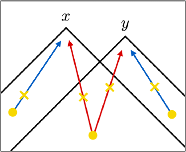
Refer to caption
Refer to caption
Figure 17: Past v𝑣v-cones relevant in the calculation beyond the envelope. Bubble wall fragments are now subject to the interception dynamics, which occurs at the points denoted by the yellow crosses. For the double-bubble contribution (blue) x𝑥x and y𝑦y are not necessarily spacelike, in contrast to the envelope case. On the other hand, for the single-bubble contribution (red), x𝑥x and y𝑦y must be spacelike because otherwise the nucleation region δVxy𝛿subscript𝑉𝑥𝑦\delta V_{xy} does not exist. See also Fig. 18 for how the left panel looks in 1+2121+2 dimensions.
Refer to caption
Figure 18: How the left panel of Fig. 17 looks in 1+2121+2 dimensions.

B.3 Single-bubble spectrum

Classification

Now we start the calculation of the single-bubble contribution. See Figs. 17 and 18. Note that x𝑥x- and y𝑦y-fragments come from the same nucleation point, and therefore, we can safely limit ourselves to the spacelike combinations of (x,y)𝑥𝑦(x,y). The single-bubble contribution can be classified into four classes, depending on whether the fragments have already been intercepted or not at the evaluation points:

  • CC𝐶𝐶CC : Both x𝑥x and y𝑦y-fragments have already collided with other bubbles at the evaluation points x𝑥x and y𝑦y.

  • CU𝐶𝑈CU : Only x𝑥x-fragment has already collided with other bubbles and y𝑦y-fragment remains uncollided at the evaluation points x𝑥x and y𝑦y.

  • UC𝑈𝐶UC : Only y𝑦y-fragment has already collided with other bubbles and x𝑥x-fragment remains uncollided at the evaluation points x𝑥x and y𝑦y.

  • UU𝑈𝑈UU : Both x𝑥x and y𝑦y-fragments remain uncollided at the evaluation points x𝑥x and y𝑦y.

In the following, we see that the single-bubble spectrum reduces to a simple expression after summing up all these classes.

Simplification formula

In this subsection we introduce a “simplification formula”, which makes the sum of the four contributions much simpler.

Let us suppose that the UU𝑈𝑈UU contribution to the correlator T(x)T(y)delimited-⟨⟩𝑇𝑥𝑇𝑦\left<T(x)T(y)\right> is written as

Tij(x)Tkl(y)(s,UU)superscriptdelimited-⟨⟩subscript𝑇𝑖𝑗𝑥subscript𝑇𝑘𝑙𝑦𝑠𝑈𝑈\displaystyle\left<T_{ij}(x)T_{kl}(y)\right>^{(s,UU)} =tmaxdtn02πdϕneI(x,y)(s)(x,y;xi=x,yi=y;zn),\displaystyle=\int_{-\infty}^{t_{\rm max}}dt_{n}\int_{0}^{2\pi}d\phi_{n}\;e^{-I(x,y)}{\mathcal{F}}^{(s)}(x,y;x_{i}=x,y_{i}=y;z_{n}), (B.6)

with some function (s)superscript𝑠{\mathcal{F}}^{(s)}. We denote the common nucleation point for x𝑥x and y𝑦y-fragments by zn=(tn,zn)subscript𝑧𝑛subscript𝑡𝑛subscript𝑧𝑛z_{n}=(t_{n},\vec{z}_{n}), which means xn=yn=znsubscript𝑥𝑛subscript𝑦𝑛subscript𝑧𝑛x_{n}=y_{n}=z_{n}. Also, ϕnsubscriptitalic-ϕ𝑛\phi_{n} is the azimuthal angle for the nucleation point znsubscript𝑧𝑛\vec{z}_{n} with respect to rxy𝑟𝑥𝑦\vec{r}\equiv\vec{x}-\vec{y}. Note that tnsubscript𝑡𝑛t_{n} and ϕnsubscriptitalic-ϕ𝑛\phi_{n} completely specify the nucleation point znsubscript𝑧𝑛z_{n} for given x𝑥x and y𝑦y. The explicit expression for (s)superscript𝑠{\mathcal{F}}^{(s)} is found in the same way as Appendix A, except that the energy-momentum tensor is now given by Eq. (2.16) with ρBsubscript𝜌𝐵\rho_{B} being Eq. (B.1):

(s)(x,y;xi,yi;zn)superscript𝑠𝑥𝑦subscript𝑥𝑖subscript𝑦𝑖subscript𝑧𝑛\displaystyle{\mathcal{F}}^{(s)}(x,y;x_{i},y_{i};z_{n})
=rlB2sin(θxn×θyn×)Γ(tn)(4π3rxn(s)3κρ014πrxn(s)2lB)(4π3ryn(s)3κρ014πryn(s)2lB)Nn×,ijklabsentsubscript𝑟perpendicular-tosuperscriptsubscript𝑙𝐵2subscript𝜃𝑥𝑛subscript𝜃𝑦𝑛Γsubscript𝑡𝑛4𝜋3superscriptsubscript𝑟𝑥𝑛𝑠3𝜅subscript𝜌014𝜋superscriptsubscript𝑟𝑥𝑛𝑠2subscript𝑙𝐵4𝜋3superscriptsubscript𝑟𝑦𝑛𝑠3𝜅subscript𝜌014𝜋superscriptsubscript𝑟𝑦𝑛𝑠2subscript𝑙𝐵subscript𝑁𝑛𝑖𝑗𝑘𝑙\displaystyle\;\;\;\;=\frac{r_{\perp}l_{B}^{2}}{\sin(\theta_{xn\times}-\theta_{yn\times})}\Gamma(t_{n})\left(\frac{4\pi}{3}r_{xn}^{(s)3}\kappa\rho_{0}\frac{1}{4\pi r_{xn}^{(s)2}l_{B}}\right)\left(\frac{4\pi}{3}r_{yn}^{(s)3}\kappa\rho_{0}\frac{1}{4\pi r_{yn}^{(s)2}l_{B}}\right)N_{n\times,ijkl}
×rB(txi,tn)3rxn(s)3rB(tyi,tn)3ryn(s)3D(tx,txi,tn)D(ty,tyi,tn).absentsubscript𝑟𝐵superscriptsubscript𝑡𝑥𝑖subscript𝑡𝑛3superscriptsubscript𝑟𝑥𝑛𝑠3subscript𝑟𝐵superscriptsubscript𝑡𝑦𝑖subscript𝑡𝑛3superscriptsubscript𝑟𝑦𝑛𝑠3𝐷subscript𝑡𝑥subscript𝑡𝑥𝑖subscript𝑡𝑛𝐷subscript𝑡𝑦subscript𝑡𝑦𝑖subscript𝑡𝑛\displaystyle\;\;\;\;\;\;\;\;\times\frac{r_{B}(t_{xi},t_{n})^{3}}{r_{xn}^{(s)3}}\frac{r_{B}(t_{yi},t_{n})^{3}}{r_{yn}^{(s)3}}D(t_{x},t_{xi},t_{n})D(t_{y},t_{yi},t_{n}). (B.7)

Here rxn(s)=rB(tx,tn)superscriptsubscript𝑟𝑥𝑛𝑠subscript𝑟𝐵subscript𝑡𝑥subscript𝑡𝑛r_{xn}^{(s)}=r_{B}(t_{x},t_{n}) and ryn(s)=rB(ty,tn)superscriptsubscript𝑟𝑦𝑛𝑠subscript𝑟𝐵subscript𝑡𝑦subscript𝑡𝑛r_{yn}^{(s)}=r_{B}(t_{y},t_{n}), and rsubscript𝑟perpendicular-tor_{\perp} and Nn×,ijklsubscript𝑁𝑛𝑖𝑗𝑘𝑙N_{n\times,ijkl} are defined in the same way as Appendix A.3. Note that substituting xi=xsubscript𝑥𝑖𝑥x_{i}=x and yi=ysubscript𝑦𝑖𝑦y_{i}=y reproduces the result with the envelope approximation (A.20). Then, interestingly, the sum of the four contributions reduces to

T(x)T(y)(s,UU+UC+CU+CC)superscriptdelimited-⟨⟩𝑇𝑥𝑇𝑦𝑠𝑈𝑈𝑈𝐶𝐶𝑈𝐶𝐶\displaystyle\left<T(x)T(y)\right>^{(s,UU+UC+CU+CC)}
=tmax𝑑tn02π𝑑ϕntxntx𝑑txitynty𝑑tyieI(xi,yi)[(s)(x,y;xi,yi,zn)]txi,tyi.absentsuperscriptsubscriptsubscript𝑡maxdifferential-dsubscript𝑡𝑛superscriptsubscript02𝜋differential-dsubscriptitalic-ϕ𝑛superscriptsubscriptsubscript𝑡𝑥𝑛subscript𝑡𝑥differential-dsubscript𝑡𝑥𝑖superscriptsubscriptsubscript𝑡𝑦𝑛subscript𝑡𝑦differential-dsubscript𝑡𝑦𝑖superscript𝑒𝐼subscript𝑥𝑖subscript𝑦𝑖subscriptdelimited-[]superscript𝑠𝑥𝑦subscript𝑥𝑖subscript𝑦𝑖subscript𝑧𝑛𝑡𝑥𝑖𝑡𝑦𝑖\displaystyle\;\;\;\;\;\;\;\;=\int_{-\infty}^{t_{\rm max}}dt_{n}\int_{0}^{2\pi}d\phi_{n}\int_{t_{xn}}^{t_{x}}dt_{xi}\int_{t_{yn}}^{t_{y}}dt_{yi}\;e^{-I(x_{i},y_{i})}\left[{\mathcal{F}}^{(s)}(x,y;x_{i},y_{i},z_{n})\right]_{txi,tyi}. (B.8)

We prove this formula in Appendix C. Here, the expression []txi,tyisubscriptdelimited-[]𝑡𝑥𝑖𝑡𝑦𝑖\left[{\mathcal{F}}\right]_{txi,tyi} denotes taking the derivatives with respect to txisubscript𝑡𝑥𝑖t_{xi} and tyisubscript𝑡𝑦𝑖t_{yi} along the propagation of the bubble wall fragments, as explained in the previous subsection. In the present case, (s)superscript𝑠{\mathcal{F}}^{(s)} in Eq. (B.8) contains the argument xi=(txi,xi)subscript𝑥𝑖subscript𝑡𝑥𝑖subscript𝑥𝑖x_{i}=(t_{xi},\vec{x}_{i}) and yi=(tyi,yi)subscript𝑦𝑖subscript𝑡𝑦𝑖subscript𝑦𝑖y_{i}=(t_{yi},\vec{y}_{i}). When taking derivatives with respect to txisubscript𝑡𝑥𝑖t_{xi} and tyisubscript𝑡𝑦𝑖t_{yi}, we regard xisubscript𝑥𝑖\vec{x}_{i} and yisubscript𝑦𝑖\vec{y}_{i} as functions of them. This is possible once the propagation directions of x𝑥x and y𝑦y-fragments are specified, and in fact they are specified by the variables tnsubscript𝑡𝑛t_{n} and ϕnsubscriptitalic-ϕ𝑛\phi_{n}.

Expressions for GW spectrum

Let us derive concrete expressions for Π(s)superscriptΠ𝑠\Pi^{(s)} and Δ(s)superscriptΔ𝑠\Delta^{(s)}. First, for a general nucleation rate ΓΓ\Gamma and the damping function D𝐷D, we obtain the following for Π(s)superscriptΠ𝑠\Pi^{(s)} by using the simplification formula (B.8):

Π(s)(tx,ty,k)=superscriptΠ𝑠subscript𝑡𝑥subscript𝑡𝑦𝑘absent\displaystyle\Pi^{(s)}(t_{x},t_{y},k)= v|tx,y|𝑑rtmax𝑑tntntx𝑑txitnty𝑑tyisuperscriptsubscript𝑣subscript𝑡𝑥𝑦differential-d𝑟superscriptsubscriptsubscript𝑡maxdifferential-dsubscript𝑡𝑛superscriptsubscriptsubscript𝑡𝑛subscript𝑡𝑥differential-dsubscript𝑡𝑥𝑖superscriptsubscriptsubscript𝑡𝑛subscript𝑡𝑦differential-dsubscript𝑡𝑦𝑖\displaystyle\int_{v|t_{x,y}|}^{\infty}dr\int_{-\infty}^{t_{\rm max}}dt_{n}\int_{t_{n}}^{t_{x}}dt_{xi}\int_{t_{n}}^{t_{y}}dt_{yi}
4π29κ2ρ024superscript𝜋29superscript𝜅2superscriptsubscript𝜌02\displaystyle\frac{4\pi^{2}}{9}\kappa^{2}\rho_{0}^{2} [eI(xi,yi)Γ(tn)rrxn(s)ryn(s)×[j0(kr)𝒦0(nxn×,nyn×)+j1(kr)kr𝒦1(nxn×,nyn×)+j2(kr)(kr)2𝒦2(nxn×,nyn×)]×txi[rB(txi,tn)3D(tx,txi,tn)]tyi[rB(tyi,tn)3D(ty,tyi,tn)]]\displaystyle\left[\begin{matrix}[l]\displaystyle\;e^{-I(x_{i},y_{i})}\;\Gamma(t_{n})\;\frac{r}{r_{xn}^{(s)}r_{yn}^{(s)}}\\ \displaystyle\times\left[j_{0}(kr){\mathcal{K}}_{0}(n_{xn\times},n_{yn\times})+\frac{j_{1}(kr)}{kr}{\mathcal{K}}_{1}(n_{xn\times},n_{yn\times})+\frac{j_{2}(kr)}{(kr)^{2}}{\mathcal{K}}_{2}(n_{xn\times},n_{yn\times})\right]\\[10.76385pt] \displaystyle\times\;\partial_{txi}\left[r_{B}(t_{xi},t_{n})^{3}D(t_{x},t_{xi},t_{n})\right]\partial_{tyi}\left[r_{B}(t_{yi},t_{n})^{3}D(t_{y},t_{yi},t_{n})\right]\end{matrix}\right] (B.9)

and the following for Δ(s)superscriptΔ𝑠\Delta^{(s)}:

Δ(s)=superscriptΔ𝑠absent\displaystyle\Delta^{(s)}= 𝑑tx𝑑tyv|tx,y|𝑑rtmax𝑑tntntx𝑑txitnty𝑑tyisuperscriptsubscriptdifferential-dsubscript𝑡𝑥superscriptsubscriptdifferential-dsubscript𝑡𝑦superscriptsubscript𝑣subscript𝑡𝑥𝑦differential-d𝑟superscriptsubscriptsubscript𝑡maxdifferential-dsubscript𝑡𝑛superscriptsubscriptsubscript𝑡𝑛subscript𝑡𝑥differential-dsubscript𝑡𝑥𝑖superscriptsubscriptsubscript𝑡𝑛subscript𝑡𝑦differential-dsubscript𝑡𝑦𝑖\displaystyle\int_{-\infty}^{\infty}dt_{x}\int_{-\infty}^{\infty}dt_{y}\int_{v|t_{x,y}|}^{\infty}dr\int_{-\infty}^{t_{\rm max}}dt_{n}\int_{t_{n}}^{t_{x}}dt_{xi}\int_{t_{n}}^{t_{y}}dt_{yi}
k33superscript𝑘33\displaystyle\frac{k^{3}}{3} [eI(xi,yi)Γ(tn)rrxn(s)ryn(s)×[j0(kr)𝒦0(nxn×,nyn×)+j1(kr)kr𝒦1(nxn×,nyn×)+j2(kr)(kr)2𝒦2(nxn×,nyn×)]×txi[rB(txi,tn)3D(tx,txi,tn)]tyi[rB(tyi,tn)3D(ty,tyi,tn)]cos(ktx,y)].\displaystyle\left[\begin{matrix}[l]\displaystyle\;e^{-I(x_{i},y_{i})}\;\Gamma(t_{n})\;\frac{r}{r_{xn}^{(s)}r_{yn}^{(s)}}\\ \displaystyle\times\left[j_{0}(kr){\mathcal{K}}_{0}(n_{xn\times},n_{yn\times})+\frac{j_{1}(kr)}{kr}{\mathcal{K}}_{1}(n_{xn\times},n_{yn\times})+\frac{j_{2}(kr)}{(kr)^{2}}{\mathcal{K}}_{2}(n_{xn\times},n_{yn\times})\right]\\[10.76385pt] \displaystyle\times\;\partial_{txi}\left[r_{B}(t_{xi},t_{n})^{3}D(t_{x},t_{xi},t_{n})\right]\partial_{tyi}\left[r_{B}(t_{yi},t_{n})^{3}D(t_{y},t_{yi},t_{n})\right]\cos(kt_{x,y})\end{matrix}\right]. (B.10)

Some comments are in order. First, the r/sin(θxn×θyn×)subscript𝑟perpendicular-tosubscript𝜃𝑥𝑛subscript𝜃𝑦𝑛r_{\perp}/\sin(\theta_{xn\times}-\theta_{yn\times}) term in Eq. (B.7) has been simplified by using the same transformations as around Eq. (A.18). Next, the derivatives with respect to the propagation directions in Eq. (B.8) are now reduced to partial derivatives. This is because txisubscript𝑡𝑥𝑖t_{xi} (tyisubscript𝑡𝑦𝑖t_{yi}) dependence of xisubscript𝑥𝑖\vec{x}_{i} (yisubscript𝑦𝑖\vec{y}_{i}) is encoded in Eq. (B.7) through rB(txi,tn)subscript𝑟𝐵subscript𝑡𝑥𝑖subscript𝑡𝑛r_{B}(t_{xi},t_{n}) (rB(tyi,tn)subscript𝑟𝐵subscript𝑡𝑦𝑖subscript𝑡𝑛r_{B}(t_{yi},t_{n})). After reducing the derivatives to partial derivatives, we can perform the integration with respect to ϕnsubscriptitalic-ϕ𝑛\phi_{n}. Finally, the integration regions are determined as follows. For r𝑟r, the lower limit is set because δVxy𝛿subscript𝑉𝑥𝑦\delta V_{xy} does not exist for r<v|txy|𝑟𝑣subscript𝑡𝑥𝑦r<v|t_{xy}|. See 17 and 18, and also the explanation at the beginning of Sec. B.3. The upper limit for tnsubscript𝑡𝑛t_{n} integration comes from the same reason. Also, the integration regions for txisubscript𝑡𝑥𝑖t_{xi} and tyisubscript𝑡𝑦𝑖t_{yi} come from the simplification formula (B.8).

Here it would be a good exercise to check that these expressions coincide with the expressions with the envelope approximation (A.21) and (A.22) if we assume an instant damping of the wall energy. Such a setup is realized by setting D(t,ti,tn)=Θ(tit+ϵ)𝐷𝑡subscript𝑡𝑖subscript𝑡𝑛Θsubscript𝑡𝑖𝑡italic-ϵD(t,t_{i},t_{n})=\Theta(t_{i}-t+\epsilon) with ϵitalic-ϵ\epsilon being infinitesimal and positive. With this form, D𝐷D is unity for time t𝑡t before ti+ϵsubscript𝑡𝑖italic-ϵt_{i}+\epsilon, while it vanishes after that. The txisubscript𝑡𝑥𝑖t_{xi} and tyisubscript𝑡𝑦𝑖t_{yi} derivatives in Eqs. (B.9) and (B.10) can act both on rBsubscript𝑟𝐵r_{B} and D𝐷D, but if either of them acts on rBsubscript𝑟𝐵r_{B} the integrand vanishes because D𝐷D is unity only for the integration range txϵ<txi<txsubscript𝑡𝑥italic-ϵsubscript𝑡𝑥𝑖subscript𝑡𝑥t_{x}-\epsilon<t_{xi}<t_{x} or tyϵ<tyi<tysubscript𝑡𝑦italic-ϵsubscript𝑡𝑦𝑖subscript𝑡𝑦t_{y}-\epsilon<t_{yi}<t_{y}. Therefore these derivatives have to act on D𝐷D, and this gives δ(txitx+ϵ)𝛿subscript𝑡𝑥𝑖subscript𝑡𝑥italic-ϵ\delta(t_{xi}-t_{x}+\epsilon) and δ(tyity+ϵ)𝛿subscript𝑡𝑦𝑖subscript𝑡𝑦italic-ϵ\delta(t_{yi}-t_{y}+\epsilon). Performing txisubscript𝑡𝑥𝑖t_{xi} and tyisubscript𝑡𝑦𝑖t_{yi} integrations, one sees that Eqs. (B.9) and (B.10) coincide with Eqs. (A.21) and (A.22), respectively.

Let us finally derive the expression for Δ(s)superscriptΔ𝑠\Delta^{(s)} with the damping function (2.23) and the nucleation rate (2.24). Given these specific forms we can perform one integration, because we can shift the whole system in the time direction without changing the geometry of bubbles. In fact, if we write all the time variables in Eq. (B.10) in terms of the difference from the nucleation time tnsubscript𝑡𝑛t_{n}, all the effects of time shift in the system appears in the exponent I(xi,yi)𝐼subscript𝑥𝑖subscript𝑦𝑖I(x_{i},y_{i}) and the nucleation rate Γ(tn)Γsubscript𝑡𝑛\Gamma(t_{n}).♢♢\diamondsuit41♢♢\diamondsuit41\diamondsuit41 In fact, in Eq. (B.10), rxn(s)=vtx,nsuperscriptsubscript𝑟𝑥𝑛𝑠𝑣subscript𝑡𝑥𝑛r_{xn}^{(s)}=vt_{x,n} and ryn(s)=vty,nsuperscriptsubscript𝑟𝑦𝑛𝑠𝑣subscript𝑡𝑦𝑛r_{yn}^{(s)}=vt_{y,n} contain time differences only, and 𝒦𝒦{\mathcal{K}} functions contain angular variables such as sxn×subscript𝑠𝑥𝑛s_{xn\times} and cxn×subscript𝑐𝑥𝑛c_{xn\times}, which can be written in terms of r𝑟r, tx,nsubscript𝑡𝑥𝑛t_{x,n} and ty,nsubscript𝑡𝑦𝑛t_{y,n}. Also, from rB(txi,tn)=vtxi,nsubscript𝑟𝐵subscript𝑡𝑥𝑖subscript𝑡𝑛𝑣subscript𝑡𝑥𝑖𝑛r_{B}(t_{xi},t_{n})=vt_{xi,n}, rB(tyi,tn)=vtyi,nsubscript𝑟𝐵subscript𝑡𝑦𝑖subscript𝑡𝑛𝑣subscript𝑡𝑦𝑖𝑛r_{B}(t_{yi},t_{n})=vt_{yi,n}, D(tx,txi,tn)=etx,xi/τ𝐷subscript𝑡𝑥subscript𝑡𝑥𝑖subscript𝑡𝑛superscript𝑒subscript𝑡𝑥𝑥𝑖𝜏D(t_{x},t_{xi},t_{n})=e^{-t_{x,xi}/\tau} and D(ty,tyi,tn)=ety,yi/τ𝐷subscript𝑡𝑦subscript𝑡𝑦𝑖subscript𝑡𝑛superscript𝑒subscript𝑡𝑦𝑦𝑖𝜏D(t_{y},t_{yi},t_{n})=e^{-t_{y,yi}/\tau}, one sees that the last line also has time differences only. Therefore we can integrate out the time shift direction and obtain

Δ(s)=superscriptΔ𝑠absent\displaystyle\Delta^{(s)}= 𝑑tx,y|tx,y|𝑑rvrv/2𝑑tx,y,n0tx,n𝑑txi,n0ty,n𝑑tyi,nsuperscriptsubscriptdifferential-dsubscript𝑡𝑥𝑦superscriptsubscriptsubscript𝑡𝑥𝑦differential-dsubscript𝑟𝑣superscriptsubscriptsubscript𝑟𝑣2differential-dsubscript𝑡𝑥𝑦𝑛superscriptsubscript0subscript𝑡𝑥𝑛differential-dsubscript𝑡𝑥𝑖𝑛superscriptsubscript0subscript𝑡𝑦𝑛differential-dsubscript𝑡𝑦𝑖𝑛\displaystyle\int_{-\infty}^{\infty}dt_{x,y}\int_{|t_{x,y}|}^{\infty}dr_{v}\int_{r_{v}/2}^{\infty}dt_{\left<x,y\right>,n}\int_{0}^{t_{x,n}}dt_{xi,n}\int_{0}^{t_{y,n}}dt_{yi,n}
v3k33superscript𝑣3superscript𝑘33\displaystyle\frac{v^{3}k^{3}}{3} [e(txi,n+tyi,n)/2e(tx,xi+ty,yi)/τ(txi,yi,rxi,yi/v)(3txi,n2+txi,n3/τ)(3tyi,n2+tyi,n3/τ)tx,nty,n×rv[j0(vkrv)𝒦0(nxn×,nyn×)+j1(vkrv)vkrv𝒦1(nxn×,nyn×)+j2(vkrv)(vkrv)2𝒦2(nxn×,nyn×)]×cos(k(tx,nty,n))].delimited-[]matrixsuperscript𝑒subscript𝑡𝑥𝑖𝑛subscript𝑡𝑦𝑖𝑛2superscript𝑒subscript𝑡𝑥𝑥𝑖subscript𝑡𝑦𝑦𝑖𝜏subscript𝑡𝑥𝑖𝑦𝑖subscript𝑟𝑥𝑖𝑦𝑖𝑣3superscriptsubscript𝑡𝑥𝑖𝑛2superscriptsubscript𝑡𝑥𝑖𝑛3𝜏3superscriptsubscript𝑡𝑦𝑖𝑛2superscriptsubscript𝑡𝑦𝑖𝑛3𝜏subscript𝑡𝑥𝑛subscript𝑡𝑦𝑛absentsubscript𝑟𝑣delimited-[]subscript𝑗0𝑣𝑘subscript𝑟𝑣subscript𝒦0subscript𝑛𝑥𝑛subscript𝑛𝑦𝑛subscript𝑗1𝑣𝑘subscript𝑟𝑣𝑣𝑘subscript𝑟𝑣subscript𝒦1subscript𝑛𝑥𝑛subscript𝑛𝑦𝑛subscript𝑗2𝑣𝑘subscript𝑟𝑣superscript𝑣𝑘subscript𝑟𝑣2subscript𝒦2subscript𝑛𝑥𝑛subscript𝑛𝑦𝑛absent𝑘subscript𝑡𝑥𝑛subscript𝑡𝑦𝑛\displaystyle\left[\begin{matrix}[l]\displaystyle\;\frac{e^{-(t_{xi,n}+t_{yi,n})/2}e^{-(t_{x,xi}+t_{y,yi})/\tau}}{{\mathcal{I}}(t_{xi,yi},r_{xi,yi}/v)}\frac{(3t_{xi,n}^{2}+t_{xi,n}^{3}/\tau)(3t_{yi,n}^{2}+t_{yi,n}^{3}/\tau)}{t_{x,n}t_{y,n}}\\[8.61108pt] \displaystyle\times\;r_{v}\left[j_{0}(vkr_{v}){\mathcal{K}}_{0}(n_{xn\times},n_{yn\times})+\frac{j_{1}(vkr_{v})}{vkr_{v}}{\mathcal{K}}_{1}(n_{xn\times},n_{yn\times})+\frac{j_{2}(vkr_{v})}{(vkr_{v})^{2}}{\mathcal{K}}_{2}(n_{xn\times},n_{yn\times})\right]\\[8.61108pt] \displaystyle\times\cos(k(t_{x,n}-t_{y,n}))\end{matrix}\right]. (B.11)

Note that tx,nsubscript𝑡𝑥𝑛t_{x,n}, ty,nsubscript𝑡𝑦𝑛t_{y,n}, tx,xisubscript𝑡𝑥𝑥𝑖t_{x,xi} and ty,yisubscript𝑡𝑦𝑦𝑖t_{y,yi} in this expression should be understood in terms of the integration variables as

tx,nsubscript𝑡𝑥𝑛\displaystyle t_{x,n} =tx,y2+tx,y,n,ty,n=tx,y2+tx,y,n,tx,xi=tx,ntxi,n,ty,yi=ty,ntyi,n,formulae-sequenceabsentsubscript𝑡𝑥𝑦2subscript𝑡𝑥𝑦𝑛formulae-sequencesubscript𝑡𝑦𝑛subscript𝑡𝑥𝑦2subscript𝑡𝑥𝑦𝑛formulae-sequencesubscript𝑡𝑥𝑥𝑖subscript𝑡𝑥𝑛subscript𝑡𝑥𝑖𝑛subscript𝑡𝑦𝑦𝑖subscript𝑡𝑦𝑛subscript𝑡𝑦𝑖𝑛\displaystyle=\frac{t_{x,y}}{2}+t_{\left<x,y\right>,n},\;\;\;\;t_{y,n}=-\frac{t_{x,y}}{2}+t_{\left<x,y\right>,n},\;\;\;\;t_{x,xi}=t_{x,n}-t_{xi,n},\;\;\;\;t_{y,yi}=t_{y,n}-t_{yi,n}, (B.12)

where tx,y,n=tx,ytnsubscript𝑡𝑥𝑦𝑛subscript𝑡𝑥𝑦subscript𝑡𝑛t_{\left<x,y\right>,n}=t_{\left<x,y\right>}-t_{n}. In addition, the arguments txi,yi=txi,ntyi,nsubscript𝑡𝑥𝑖𝑦𝑖subscript𝑡𝑥𝑖𝑛subscript𝑡𝑦𝑖𝑛t_{xi,yi}=t_{xi,n}-t_{yi,n} and rxi,yi=|xiyi|subscript𝑟𝑥𝑖𝑦𝑖subscript𝑥𝑖subscript𝑦𝑖r_{xi,yi}=|\vec{x}_{i}-\vec{y}_{i}| in the {\mathcal{I}} function are also functions of the integration variables. In fact, using the relation xiyi=r+v(tx,xinxn×ty,yinyn×)subscript𝑥𝑖subscript𝑦𝑖𝑟𝑣subscript𝑡𝑥𝑥𝑖subscript𝑛𝑥𝑛subscript𝑡𝑦𝑦𝑖subscript𝑛𝑦𝑛\vec{x}_{i}-\vec{y}_{i}=\vec{r}+v(t_{x,xi}n_{xn\times}-t_{y,yi}n_{yn\times}) (with the subscript n𝑛n indicating that the vectors nx×subscript𝑛𝑥n_{x\times} and ny×subscript𝑛𝑦n_{y\times} are on the constant-time hypersurface ΣtnsubscriptΣsubscript𝑡𝑛\Sigma_{t_{n}}), one can express rxi,yisubscript𝑟𝑥𝑖𝑦𝑖r_{xi,yi} as

rxi,yivsubscript𝑟𝑥𝑖𝑦𝑖𝑣\displaystyle\frac{r_{xi,yi}}{v} =rv2+tx,xi2+ty,yi2+2rvtx,xicxn×2rvty,yicyn×2tx,xity,yicxyn×,absentsuperscriptsubscript𝑟𝑣2superscriptsubscript𝑡𝑥𝑥𝑖2superscriptsubscript𝑡𝑦𝑦𝑖22subscript𝑟𝑣subscript𝑡𝑥𝑥𝑖subscript𝑐𝑥𝑛2subscript𝑟𝑣subscript𝑡𝑦𝑦𝑖subscript𝑐𝑦𝑛2subscript𝑡𝑥𝑥𝑖subscript𝑡𝑦𝑦𝑖subscript𝑐𝑥𝑦𝑛\displaystyle=\sqrt{r_{v}^{2}+t_{x,xi}^{2}+t_{y,yi}^{2}+2r_{v}t_{x,xi}c_{xn\times}-2r_{v}t_{y,yi}c_{yn\times}-2t_{x,xi}t_{y,yi}c_{xyn\times}}, (B.13)

where cxn×subscript𝑐𝑥𝑛c_{xn\times} and cyn×subscript𝑐𝑦𝑛c_{yn\times} are the cosines introduced around Eq. (A.13). In addition, cxyn×subscript𝑐𝑥𝑦𝑛c_{xyn\times} is the cosine of the angle between nxn×subscript𝑛𝑥𝑛n_{xn\times} and nyn×subscript𝑛𝑦𝑛n_{yn\times} given by cxyn×=cxn×cyn×+sxn×syn×subscript𝑐𝑥𝑦𝑛subscript𝑐𝑥𝑛subscript𝑐𝑦𝑛subscript𝑠𝑥𝑛subscript𝑠𝑦𝑛c_{xyn\times}=c_{xn\times}c_{yn\times}+s_{xn\times}s_{yn\times}. Alternatively, using xiyi=v(txi,nnxn×+tyi,nnyn×)subscript𝑥𝑖subscript𝑦𝑖𝑣subscript𝑡𝑥𝑖𝑛subscript𝑛𝑥𝑛subscript𝑡𝑦𝑖𝑛subscript𝑛𝑦𝑛\vec{x}_{i}-\vec{y}_{i}=v(-t_{xi,n}n_{xn\times}+t_{yi,n}n_{yn\times}), one has

rxi,yivsubscript𝑟𝑥𝑖𝑦𝑖𝑣\displaystyle\frac{r_{xi,yi}}{v} =txi,n2+tyi,n22txi,ntyi,ncxyn×,absentsuperscriptsubscript𝑡𝑥𝑖𝑛2superscriptsubscript𝑡𝑦𝑖𝑛22subscript𝑡𝑥𝑖𝑛subscript𝑡𝑦𝑖𝑛subscript𝑐𝑥𝑦𝑛\displaystyle=\sqrt{t_{xi,n}^{2}+t_{yi,n}^{2}-2t_{xi,n}t_{yi,n}c_{xyn\times}}, (B.14)

which also gives an expression of rxi,yisubscript𝑟𝑥𝑖𝑦𝑖r_{xi,yi} in terms of the integration variables.

B.4 Double-bubble spectrum

Classification

Next we move on to the calculation of the double-bubble contribution. We first classify bubble wall properties as in the single-bubble case. The bubble wall fragment reaching the evaluation point x𝑥x or y𝑦y is either already collided or still uncollided, as before. In the double-bubble case, however, we need further classification for the former depending on whether the bubble which intercepts the x𝑥x-(or y𝑦y-)fragment is the bubble which y𝑦y-(or x𝑥x-)fragment belongs to. We illustrate this point in Fig. 19. The horizontal (vertical) axis is the space (time) direction, and the blue arrows denote the propagation of the x𝑥x- and y𝑦y-fragments. Note that these blue arrows are propagating on the surface of v𝑣v-cones as in Fig. 18. In the upper-left panel, the interception (denoted by the crosses) occurs to the x𝑥x-(or y𝑦y-)fragment (denoted by blue arrows) before the wall of the y𝑦y-(or x𝑥x-)bubble (denoted by yellow lines) catches up with the x𝑥x-(or y𝑦y-)fragment. In such cases the intercepting bubble is different from the one which the other fragment belongs to, and we label such contribution by Ci×Cisubscript𝐶𝑖subscript𝐶𝑖C_{i}\times C_{i}. The opposite case is shown in the lower-right panel, where x𝑥x-(y𝑦y-)fragment is intercepted by the bubble wall which the other fragment belongs to. We label such contributions by Cin×Cinsubscript𝐶𝑖𝑛subscript𝐶𝑖𝑛C_{in}\times C_{in}. The meaning of the other two cases Ci×Cinsubscript𝐶𝑖subscript𝐶𝑖𝑛C_{i}\times C_{in} and Cin×Cisubscript𝐶𝑖𝑛subscript𝐶𝑖C_{in}\times C_{i} is now trivial. Note that whether contributions including Cinsubscript𝐶𝑖𝑛C_{in} exist or not depends on the choice of the spacetime points x𝑥x and y𝑦y and on the choice of the propagation directions.

In summary, we can classify the double-bubble contribution into (U,Ci,Cin)×(U,Ci,Cin)𝑈subscript𝐶𝑖subscript𝐶𝑖𝑛𝑈subscript𝐶𝑖subscript𝐶𝑖𝑛(U,C_{i},C_{in})\times(U,C_{i},C_{in}), where

  • U𝑈U : x𝑥x-(or y𝑦y-)fragment remains uncollided at the evaluation point.

  • Cisubscript𝐶𝑖C_{i} : x𝑥x-(or y𝑦y-)fragment has already been intercepted at the evaluation point, and the interception occurs with a collision with a bubble other than the y𝑦y-(or x𝑥x-)bubble.

  • Cinsubscript𝐶𝑖𝑛C_{in} : x𝑥x-(or y𝑦y-)fragment has already been intercepted at the evaluation point, and the interception occurs with a collision with the y𝑦y-(or x𝑥x-)bubble.

One may notice that Ci×Cisubscript𝐶𝑖subscript𝐶𝑖C_{i}\times C_{i} contribution can be classified into two classes: the intercepting bubbles for the x𝑥x- and y𝑦y-fragments are identical or not. Both of them can properly be taken into account by the simplification formula we explain below.
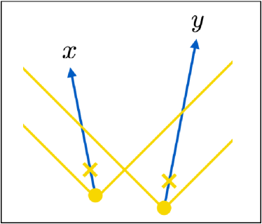
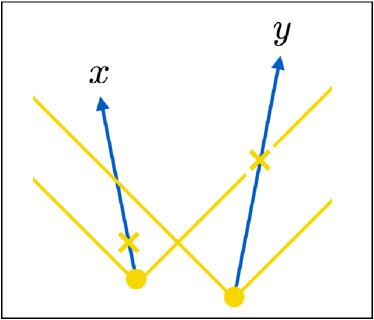
Refer to caption
Refer to caption
Refer to caption
Refer to caption
Figure 19: Illustration for (Ci,Cin)×(Ci,Cin)subscript𝐶𝑖subscript𝐶𝑖𝑛subscript𝐶𝑖subscript𝐶𝑖𝑛(C_{i},C_{in})\times(C_{i},C_{in}) in the double-bubble contribution. The circles denote the nucleation points for the x𝑥x- and y𝑦y-fragments, which are shown in blue arrows. The crosses on these arrows denote the interception points for these fragments. Note that some choices of x𝑥x and y𝑦y forbid the three types including Cinsubscript𝐶𝑖𝑛C_{in} (i.e. CiCinsubscript𝐶𝑖subscript𝐶𝑖𝑛C_{i}C_{in}, CinCisubscript𝐶𝑖𝑛subscript𝐶𝑖C_{in}C_{i} and CinCinsubscript𝐶𝑖𝑛subscript𝐶𝑖𝑛C_{in}C_{in}). (Top-left) CiCisubscript𝐶𝑖subscript𝐶𝑖C_{i}C_{i}: the intercepting bubbles for the x𝑥x- and y𝑦y-fragments are different from the y𝑦y- and x𝑥x-bubbles, respectively. (Top-right) CiCinsubscript𝐶𝑖subscript𝐶𝑖𝑛C_{i}C_{in}: the intercepting bubble for the y𝑦y-fragment is the x𝑥x-bubble. (Bottom-left) CinCisubscript𝐶𝑖𝑛subscript𝐶𝑖C_{in}C_{i}: the intercepting bubble for the y𝑦y-fragment is the y𝑦y-bubble. (Bottom-right) CinCinsubscript𝐶𝑖𝑛subscript𝐶𝑖𝑛C_{in}C_{in}: the intercepting bubbles for the x𝑥x- and y𝑦y-fragments are the y𝑦y- and x𝑥x bubbles, respectively.

Simplification formula

A simplification formula exists in the double-bubble case as well, which makes the sum of the nine classes (U,Ci,Cin)×(U,Ci,Cin)𝑈subscript𝐶𝑖subscript𝐶𝑖𝑛𝑈subscript𝐶𝑖subscript𝐶𝑖𝑛(U,C_{i},C_{in})\times(U,C_{i},C_{in}) much simpler. First, let us write the UU𝑈𝑈UU contribution in the following form:

Tij(x)Tkl(y)(d,UU)superscriptdelimited-⟨⟩subscript𝑇𝑖𝑗𝑥subscript𝑇𝑘𝑙𝑦𝑑𝑈𝑈\displaystyle\left<T_{ij}(x)T_{kl}(y)\right>^{(d,UU)} =tx𝑑txnty𝑑tyn𝑑Ωxn𝑑Ωynabsentsuperscriptsubscriptsubscript𝑡𝑥differential-dsubscript𝑡𝑥𝑛superscriptsubscriptsubscript𝑡𝑦differential-dsubscript𝑡𝑦𝑛differential-dsubscriptΩ𝑥𝑛differential-dsubscriptΩ𝑦𝑛\displaystyle=\int_{-\infty}^{t_{x}}dt_{xn}\int_{-\infty}^{t_{y}}dt_{yn}\int d\Omega_{xn}\int d\Omega_{yn}\;
Θsp(x,yn)Θsp(xn,y)eI(x,y)(d)(x,y;xi=x,yi=y;xn,yn).\displaystyle\;\;\;\;\;\;\Theta_{\rm sp}(x,y_{n})\Theta_{\rm sp}(x_{n},y)e^{-I(x,y)}{\mathcal{F}}^{(d)}(x,y;x_{i}=x,y_{i}=y;x_{n},y_{n}). (B.15)

Here ΩxnsubscriptΩ𝑥𝑛\Omega_{xn} and ΩynsubscriptΩ𝑦𝑛\Omega_{yn} denote the propagation directions (θxn,ϕxn)subscript𝜃𝑥𝑛subscriptitalic-ϕ𝑥𝑛(\theta_{xn},\phi_{xn}) and (θyn,ϕyn)subscript𝜃𝑦𝑛subscriptitalic-ϕ𝑦𝑛(\theta_{yn},\phi_{yn}) of the wall fragments, respectively. Note that the constant-time hypersurfaces at the nucleation times differ for x𝑥x- and y𝑦y-bubbles, since the nucleation of x𝑥x- and y𝑦y-bubbles occurs independently of each other. This argument is the same as Appendix A.4. On the other hand, the integration ranges for these directions are now over the whole solid angle in Eq. (B.15) in contrast to Appendix A.4. In Appendix A.4 we integrate the nucleation points over δVx(y)=δVxVy𝛿superscriptsubscript𝑉𝑥𝑦𝛿subscript𝑉𝑥subscript𝑉𝑦\delta V_{x}^{(y)}=\delta V_{x}-V_{y} and δVy(x)=δVyVx𝛿superscriptsubscript𝑉𝑦𝑥𝛿subscript𝑉𝑦subscript𝑉𝑥\delta V_{y}^{(x)}=\delta V_{y}-V_{x}, which do not form the whole solid angle. This might seem contradictory, but actually is not. The spacelike theta functions in Eq. (B.15) guarantee that the integration ranges are effectively the same. We illustrate this point in Fig. 20. The nucleation point xnsubscript𝑥𝑛x_{n} cannot enter the past v𝑣v-cone of y𝑦y because Θsp(xn,y)subscriptΘspsubscript𝑥𝑛𝑦\Theta_{\rm sp}(x_{n},y) gives zero in such cases, while Θsp(x,yn)subscriptΘsp𝑥subscript𝑦𝑛\Theta_{\rm sp}(x,y_{n}) guarantees that ynsubscript𝑦𝑛y_{n} is outside the v𝑣v-cone of x𝑥x. Also note that Eq. (B.15) forces (x,y)𝑥𝑦(x,y) to be spacelike, because if x𝑥x and y𝑦y are timelike the theta functions make the integrand to vanish for any solid angle. The explicit form of (d)superscript𝑑{\mathcal{F}}^{(d)} is read off from the derivation in Appendix A:

(d)(x,y;xi,yi;xn,yn)superscript𝑑𝑥𝑦subscript𝑥𝑖subscript𝑦𝑖subscript𝑥𝑛subscript𝑦𝑛\displaystyle{\mathcal{F}}^{(d)}(x,y;x_{i},y_{i};x_{n},y_{n})
=rxn(d)2lBΓ(txn)ryn(d)2lBΓ(tyn)(4π3rxn(d)3κρ014πrxn(d)2lB)(4π3ryn(d)3κρ014πryn(d)2lB)Nn,ijklabsentsuperscriptsubscript𝑟𝑥𝑛𝑑2subscript𝑙𝐵Γsubscript𝑡𝑥𝑛superscriptsubscript𝑟𝑦𝑛𝑑2subscript𝑙𝐵Γsubscript𝑡𝑦𝑛4𝜋3superscriptsubscript𝑟𝑥𝑛𝑑3𝜅subscript𝜌014𝜋superscriptsubscript𝑟𝑥𝑛𝑑2subscript𝑙𝐵4𝜋3superscriptsubscript𝑟𝑦𝑛𝑑3𝜅subscript𝜌014𝜋superscriptsubscript𝑟𝑦𝑛𝑑2subscript𝑙𝐵subscript𝑁𝑛𝑖𝑗𝑘𝑙\displaystyle\;\;\;\;=r_{xn}^{(d)2}l_{B}\Gamma(t_{xn})\;r_{yn}^{(d)2}l_{B}\Gamma(t_{yn})\left(\frac{4\pi}{3}r_{xn}^{(d)3}\kappa\rho_{0}\frac{1}{4\pi r_{xn}^{(d)2}l_{B}}\right)\left(\frac{4\pi}{3}r_{yn}^{(d)3}\kappa\rho_{0}\frac{1}{4\pi r_{yn}^{(d)2}l_{B}}\right)N_{n,ijkl}
×rB(txi,txn)3rxn(d)3rB(tyi,tyn)3ryn(d)3D(tx,txi,txn)D(ty,tyi,tyn).absentsubscript𝑟𝐵superscriptsubscript𝑡𝑥𝑖subscript𝑡𝑥𝑛3superscriptsubscript𝑟𝑥𝑛𝑑3subscript𝑟𝐵superscriptsubscript𝑡𝑦𝑖subscript𝑡𝑦𝑛3superscriptsubscript𝑟𝑦𝑛𝑑3𝐷subscript𝑡𝑥subscript𝑡𝑥𝑖subscript𝑡𝑥𝑛𝐷subscript𝑡𝑦subscript𝑡𝑦𝑖subscript𝑡𝑦𝑛\displaystyle\;\;\;\;\;\;\;\;\times\frac{r_{B}(t_{xi},t_{xn})^{3}}{r_{xn}^{(d)3}}\frac{r_{B}(t_{yi},t_{yn})^{3}}{r_{yn}^{(d)3}}D(t_{x},t_{xi},t_{xn})D(t_{y},t_{yi},t_{yn}). (B.16)

In fact, one sees that the substitution of xi=xsubscript𝑥𝑖𝑥x_{i}=x and yi=ysubscript𝑦𝑖𝑦y_{i}=y reproduces Eq. (A.27).

Now, the sum of the nine contributions (U,Ci,Cin)×(U,Ci,Cin)𝑈subscript𝐶𝑖subscript𝐶𝑖𝑛𝑈subscript𝐶𝑖subscript𝐶𝑖𝑛(U,C_{i},C_{in})\times(U,C_{i},C_{in}) gives a simple formula

Tij(x)Tkl(y)(d,(U,Ci,Cin)×(U,Ci,Cin))superscriptdelimited-⟨⟩subscript𝑇𝑖𝑗𝑥subscript𝑇𝑘𝑙𝑦𝑑𝑈subscript𝐶𝑖subscript𝐶𝑖𝑛𝑈subscript𝐶𝑖subscript𝐶𝑖𝑛\displaystyle\left<T_{ij}(x)T_{kl}(y)\right>^{(d,(U,C_{i},C_{in})\times(U,C_{i},C_{in}))}
=tx𝑑txnty𝑑tyntxntx𝑑txitynty𝑑tyi𝑑Ωxn𝑑Ωynabsentsuperscriptsubscriptsubscript𝑡𝑥differential-dsubscript𝑡𝑥𝑛superscriptsubscriptsubscript𝑡𝑦differential-dsubscript𝑡𝑦𝑛superscriptsubscriptsubscript𝑡𝑥𝑛subscript𝑡𝑥differential-dsubscript𝑡𝑥𝑖superscriptsubscriptsubscript𝑡𝑦𝑛subscript𝑡𝑦differential-dsubscript𝑡𝑦𝑖differential-dsubscriptΩ𝑥𝑛differential-dsubscriptΩ𝑦𝑛\displaystyle\;\;\;\;\;\;\;\;=\int_{-\infty}^{t_{x}}dt_{xn}\int_{-\infty}^{t_{y}}dt_{yn}\int_{t_{xn}}^{t_{x}}dt_{xi}\int_{t_{yn}}^{t_{y}}dt_{yi}\int d\Omega_{xn}\int d\Omega_{yn}\;
Θsp(xi,yn)Θsp(xn,yi)eI(xi,yi)[(d)(x,y;xi,yi;xn,yn)]txi,tyi.subscriptΘspsubscript𝑥𝑖subscript𝑦𝑛subscriptΘspsubscript𝑥𝑛subscript𝑦𝑖superscript𝑒𝐼subscript𝑥𝑖subscript𝑦𝑖subscriptdelimited-[]superscript𝑑𝑥𝑦subscript𝑥𝑖subscript𝑦𝑖subscript𝑥𝑛subscript𝑦𝑛𝑡𝑥𝑖𝑡𝑦𝑖\displaystyle\;\;\;\;\;\;\;\;\;\;\;\;\;\;\;\;\Theta_{\rm sp}(x_{i},y_{n})\Theta_{\rm sp}(x_{n},y_{i})e^{-I(x_{i},y_{i})}\left[{\mathcal{F}}^{(d)}(x,y;x_{i},y_{i};x_{n},y_{n})\right]_{txi,tyi}. (B.17)

Here the subscript on the squared parenthesis denotes the time derivatives along the propagation of the wall fragments defined in Appendix B.2. We prove this formula in Appendix C.
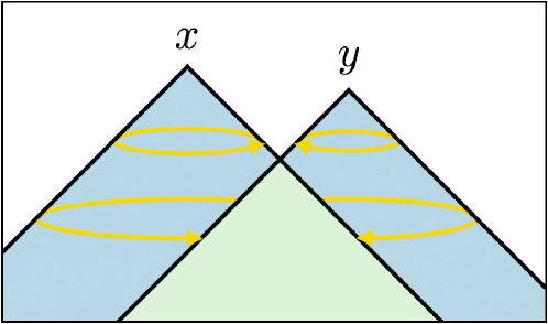
Refer to caption
Figure 20: Illustration for the integration ranges for the angular variables in Eq. (B.15). The yellow arrows show how the nucleation point changes as the propagation direction ΩxnsubscriptΩ𝑥𝑛\Omega_{xn} (ΩynsubscriptΩ𝑦𝑛\Omega_{yn}) changes on a constant-time hypersurface. For tx>tmaxsubscript𝑡𝑥subscript𝑡maxt_{x}>t_{\rm max} (ty>tmaxsubscript𝑡𝑦subscript𝑡maxt_{y}>t_{\rm max}) the spacelike theta functions in Eq. (B.15) always give unity (the upper two yellow lines), while for tx<tmaxsubscript𝑡𝑥subscript𝑡maxt_{x}<t_{\rm max} (ty<tmaxsubscript𝑡𝑦subscript𝑡maxt_{y}<t_{\rm max}) they make the integrand vanish if the nucleation point xnsubscript𝑥𝑛x_{n} (ynsubscript𝑦𝑛y_{n}) enters the past v𝑣v-cone of y𝑦y (x𝑥x) (the lower two yellow lines). Also, they always give zero for timelike combinations of x𝑥x and y𝑦y. Therefore the integration ranges are effectively constrained within δVx(y)𝛿superscriptsubscript𝑉𝑥𝑦\delta V_{x}^{(y)} and δVy(x)𝛿superscriptsubscript𝑉𝑦𝑥\delta V_{y}^{(x)} with spacelike combinations of x𝑥x and y𝑦y, and hence Eq. (B.15) is consistent with the calculation in Sec. A.4.

Expressions for GW spectrum

We now derive concrete expressions for Π(d)superscriptΠ𝑑\Pi^{(d)} and Δ(d)superscriptΔ𝑑\Delta^{(d)}. For a general nucleation rate ΓΓ\Gamma and the dumping function D𝐷D, the simplification formula (B.17) gives

Π(d)(tx,ty,k)=superscriptΠ𝑑subscript𝑡𝑥subscript𝑡𝑦𝑘absent\displaystyle\Pi^{(d)}(t_{x},t_{y},k)= 0𝑑rtx𝑑txnty𝑑tyntxntx𝑑txitynty𝑑tyi11𝑑cxn11𝑑cyn02π𝑑ϕxn,ynsuperscriptsubscript0differential-d𝑟superscriptsubscriptsubscript𝑡𝑥differential-dsubscript𝑡𝑥𝑛superscriptsubscriptsubscript𝑡𝑦differential-dsubscript𝑡𝑦𝑛superscriptsubscriptsubscript𝑡𝑥𝑛subscript𝑡𝑥differential-dsubscript𝑡𝑥𝑖superscriptsubscriptsubscript𝑡𝑦𝑛subscript𝑡𝑦differential-dsubscript𝑡𝑦𝑖superscriptsubscript11differential-dsubscript𝑐𝑥𝑛superscriptsubscript11differential-dsubscript𝑐𝑦𝑛superscriptsubscript02𝜋differential-dsubscriptitalic-ϕ𝑥𝑛𝑦𝑛\displaystyle\int_{0}^{\infty}dr\int_{-\infty}^{t_{x}}dt_{xn}\int_{-\infty}^{t_{y}}dt_{yn}\int_{t_{xn}}^{t_{x}}dt_{xi}\int_{t_{yn}}^{t_{y}}dt_{yi}\int_{-1}^{1}dc_{xn}\int_{-1}^{1}dc_{yn}\int_{0}^{2\pi}d\phi_{xn,yn}
4π29κ2ρ024superscript𝜋29superscript𝜅2superscriptsubscript𝜌02\displaystyle\frac{4\pi^{2}}{9}\kappa^{2}\rho_{0}^{2} [Θsp(xi,yn)Θsp(xn,yi)eI(xi,yi)Γ(txn)Γ(tyn)×r2[j0(kr)𝒦0(nxn,nyn)+j1(kr)kr𝒦1(nxn,nyn)+j2(kr)(kr)2𝒦2(nxn,nyn)]×txi[rB(txi,txn)3D(tx,txi,txn)]tyi[rB(tyi,tyn)3D(ty,tyi,tyn)]],\displaystyle\left[\begin{matrix}[l]\displaystyle\;\Theta_{\rm sp}(x_{i},y_{n})\Theta_{\rm sp}(x_{n},y_{i})e^{-I(x_{i},y_{i})}\Gamma(t_{xn})\Gamma(t_{yn})\\[4.30554pt] \displaystyle\times\;r^{2}\left[j_{0}(kr){\mathcal{K}}_{0}(n_{xn},n_{yn})+\frac{j_{1}(kr)}{kr}{\mathcal{K}}_{1}(n_{xn},n_{yn})+\frac{j_{2}(kr)}{(kr)^{2}}{\mathcal{K}}_{2}(n_{xn},n_{yn})\right]\\[8.61108pt] \displaystyle\times\;\partial_{txi}\left[r_{B}(t_{xi},t_{xn})^{3}D(t_{x},t_{xi},t_{xn})\right]\partial_{tyi}\left[r_{B}(t_{yi},t_{yn})^{3}D(t_{y},t_{yi},t_{yn})\right]\end{matrix}\right], (B.18)

for the correlator, and

Δ(d)=superscriptΔ𝑑absent\displaystyle\Delta^{(d)}= 𝑑tx𝑑tysuperscriptsubscriptdifferential-dsubscript𝑡𝑥superscriptsubscriptdifferential-dsubscript𝑡𝑦\displaystyle\int_{-\infty}^{\infty}dt_{x}\int_{-\infty}^{\infty}dt_{y}
0𝑑rtx𝑑txnty𝑑tyntxntx𝑑txitynty𝑑tyi11𝑑cxn11𝑑cyn02π𝑑ϕxn,ynsuperscriptsubscript0differential-d𝑟superscriptsubscriptsubscript𝑡𝑥differential-dsubscript𝑡𝑥𝑛superscriptsubscriptsubscript𝑡𝑦differential-dsubscript𝑡𝑦𝑛superscriptsubscriptsubscript𝑡𝑥𝑛subscript𝑡𝑥differential-dsubscript𝑡𝑥𝑖superscriptsubscriptsubscript𝑡𝑦𝑛subscript𝑡𝑦differential-dsubscript𝑡𝑦𝑖superscriptsubscript11differential-dsubscript𝑐𝑥𝑛superscriptsubscript11differential-dsubscript𝑐𝑦𝑛superscriptsubscript02𝜋differential-dsubscriptitalic-ϕ𝑥𝑛𝑦𝑛\displaystyle\int_{0}^{\infty}dr\int_{-\infty}^{t_{x}}dt_{xn}\int_{-\infty}^{t_{y}}dt_{yn}\int_{t_{xn}}^{t_{x}}dt_{xi}\int_{t_{yn}}^{t_{y}}dt_{yi}\int_{-1}^{1}dc_{xn}\int_{-1}^{1}dc_{yn}\int_{0}^{2\pi}d\phi_{xn,yn}
k33superscript𝑘33\displaystyle\frac{k^{3}}{3} [Θsp(xi,yn)Θsp(xn,yi)eI(xi,yi)Γ(txn)Γ(tyn)×r2[j0(kr)𝒦0(nxn,nyn)+j1(kr)kr𝒦1(nxn,nyn)+j2(kr)(kr)2𝒦2(nxn,nyn)]×txi[rB(txi,txn)3D(tx,txi,tyn)]tyi[rB(tyi,tyn)3D(ty,tyi,tyn)]cos(ktx,y)],\displaystyle\left[\begin{matrix}[l]\displaystyle\;\Theta_{\rm sp}(x_{i},y_{n})\Theta_{\rm sp}(x_{n},y_{i})e^{-I(x_{i},y_{i})}\Gamma(t_{xn})\Gamma(t_{yn})\\[4.30554pt] \displaystyle\times\;r^{2}\left[j_{0}(kr){\mathcal{K}}_{0}(n_{xn},n_{yn})+\frac{j_{1}(kr)}{kr}{\mathcal{K}}_{1}(n_{xn},n_{yn})+\frac{j_{2}(kr)}{(kr)^{2}}{\mathcal{K}}_{2}(n_{xn},n_{yn})\right]\\[8.61108pt] \displaystyle\times\;\partial_{txi}\left[r_{B}(t_{xi},t_{xn})^{3}D(t_{x},t_{xi},t_{yn})\right]\partial_{tyi}\left[r_{B}(t_{yi},t_{yn})^{3}D(t_{y},t_{yi},t_{yn})\right]\cos(kt_{x,y})\end{matrix}\right], (B.19)

for the GW spectrum. Note that the derivatives along the propagation of the wall fragments have now reduced to partial derivatives with respect to the interception times txisubscript𝑡𝑥𝑖t_{xi} and tyisubscript𝑡𝑦𝑖t_{yi}, because the dependence of xisubscript𝑥𝑖\vec{x}_{i} and yisubscript𝑦𝑖\vec{y}_{i} on txisubscript𝑡𝑥𝑖t_{xi} and tyisubscript𝑡𝑦𝑖t_{yi}, respectively, is now encoded in the functional form of (d)superscript𝑑{\mathcal{F}}^{(d)}. Also note that the integration range for r𝑟r is r>0𝑟0r>0 in contrast to Appendix A.4. As explained above, this is because the spacelike theta functions effectively guarantee that the nucleation point for the x𝑥x-(or y𝑦y-)bubble to be spacelike to the evaluation point y𝑦y (or x𝑥x). In addition, we have integrated out the azimuthal angle (ϕxn+ϕyn)/2subscriptitalic-ϕ𝑥𝑛subscriptitalic-ϕ𝑦𝑛2(\phi_{xn}+\phi_{yn})/2 because the geometry of the system is independent of this direction. This leaves ϕxn,yn=ϕxnϕynsubscriptitalic-ϕ𝑥𝑛𝑦𝑛subscriptitalic-ϕ𝑥𝑛subscriptitalic-ϕ𝑦𝑛\phi_{xn,yn}=\phi_{xn}-\phi_{yn} as the only remaining azimuthal angle.

Again it would be a good exercise to check that Eqs. (B.18) and (B.19) coincide with the expressions with the envelope approximation (A.29) and (A.30) if we assume an instant damping of the wall energy. As in Sec. B.3, we take the damping function to be D(t,ti,tn)=Θ(tit+ϵ)𝐷𝑡subscript𝑡𝑖subscript𝑡𝑛Θsubscript𝑡𝑖𝑡italic-ϵD(t,t_{i},t_{n})=\Theta(t_{i}-t+\epsilon) with ϵitalic-ϵ\epsilon being infinitesimal and positive. The txisubscript𝑡𝑥𝑖t_{xi} and tyisubscript𝑡𝑦𝑖t_{yi} derivatives have to act on the damping functions due to the same reason as the previous subsection, and we can complete txisubscript𝑡𝑥𝑖t_{xi} and tyisubscript𝑡𝑦𝑖t_{yi} integrations using the resulting delta functions. Now the spacelike theta functions are replaced by Θsp(x,yn)subscriptΘsp𝑥subscript𝑦𝑛\Theta_{\rm sp}(x,y_{n}) and Θsp(y,xn)subscriptΘsp𝑦subscript𝑥𝑛\Theta_{\rm sp}(y,x_{n}), and hence only spacelike combinations of (x,yn)𝑥subscript𝑦𝑛(x,y_{n}) and (y,xn)𝑦subscript𝑥𝑛(y,x_{n}) are allowed. Since the integration tx>tmaxsubscript𝑡𝑥subscript𝑡maxt_{x}>t_{\rm max} or ty>tmaxsubscript𝑡𝑦subscript𝑡maxt_{y}>t_{\rm max} gives vanishing contributions due to the spherical symmetry, one can safely restrict the integration range to tx<tmaxsubscript𝑡𝑥subscript𝑡maxt_{x}<t_{\rm max} and ty<tmaxsubscript𝑡𝑦subscript𝑡maxt_{y}<t_{\rm max} to obtain Eq. (A.28). The same arguments as Appendix A.4 lead to Eqs. (A.29) and (A.30).

Finally we derive the GW spectrum with the nucleation rate (2.24) and the damping function (2.23). Given these specific forms, we can perform the integration with respect to the overall time shift of the system. In fact, one can write all the time variables in Eq. (B.19) in terms of time differences except for the exponent I(xi,yi)𝐼subscript𝑥𝑖subscript𝑦𝑖I(x_{i},y_{i}) and the nucleation rate Γ(txn)Γ(tyn)Γsubscript𝑡𝑥𝑛Γsubscript𝑡𝑦𝑛\Gamma(t_{xn})\Gamma(t_{yn}). From the derivation in Appendix A.4 we know that such a time shift direction can be integrated out. As a result, we have ♢♢\diamondsuit42♢♢\diamondsuit42\diamondsuit42 In Eq. (B.19), the spacelike theta functions as well as the second and third lines in the square parenthesis contain time differences only. Therefore, overall time-shift dependence appears only in I(xi,yi)=v3Γetx,y/2e(tx,xi+ty,yirxi,yi/v)/2(txi,yi,rxi,yi)𝐼subscript𝑥𝑖subscript𝑦𝑖superscript𝑣3subscriptΓsuperscript𝑒subscript𝑡𝑥𝑦2superscript𝑒subscript𝑡𝑥𝑥𝑖subscript𝑡𝑦𝑦𝑖subscript𝑟𝑥𝑖𝑦𝑖𝑣2subscript𝑡𝑥𝑖𝑦𝑖subscript𝑟𝑥𝑖𝑦𝑖I(x_{i},y_{i})=v^{3}\Gamma_{*}e^{t_{\left<x,y\right>}/2}e^{-(t_{x,xi}+t_{y,yi}-r_{xi,yi}/v)/2}{\mathcal{I}}(t_{xi,yi},r_{xi,yi}) and the nucleation rate Γ(txn)Γ(tyn)=Γ2e2tx,ye(tx,xn+ty,yn)Γsubscript𝑡𝑥𝑛Γsubscript𝑡𝑦𝑛superscriptsubscriptΓ2superscript𝑒2subscript𝑡𝑥𝑦superscript𝑒subscript𝑡𝑥𝑥𝑛subscript𝑡𝑦𝑦𝑛\Gamma(t_{xn})\Gamma(t_{yn})=\Gamma_{*}^{2}e^{2t_{\left<x,y\right>}}e^{-(t_{x,xn}+t_{y,yn})}, in the form of etx,ysuperscript𝑒subscript𝑡𝑥𝑦e^{t_{\left<x,y\right>}}. After rewriting txsubscript𝑡𝑥t_{x} and tysubscript𝑡𝑦t_{y} integrations into tx,ysubscript𝑡𝑥𝑦t_{\left<x,y\right>} and tx,ysubscript𝑡𝑥𝑦t_{x,y} integrations, and expressing all the other time integration variables in terms of time differences like tx,xnsubscript𝑡𝑥𝑥𝑛t_{x,xn}, ty,ynsubscript𝑡𝑦𝑦𝑛t_{y,yn}, tx,xisubscript𝑡𝑥𝑥𝑖t_{x,xi} and ty,yisubscript𝑡𝑦𝑦𝑖t_{y,yi}, we can integrate out tx,ysubscript𝑡𝑥𝑦t_{\left<x,y\right>} direction to obtain Eq. (B.20).

Δ(d)=superscriptΔ𝑑absent\displaystyle\Delta^{(d)}= 𝑑tx,y0𝑑rvsuperscriptsubscriptdifferential-dsubscript𝑡𝑥𝑦superscriptsubscript0differential-dsubscript𝑟𝑣\displaystyle\int_{-\infty}^{\infty}dt_{x,y}\int_{0}^{\infty}dr_{v}
0𝑑tx,xn0𝑑ty,yn0tx,xn𝑑tx,xi0ty,yn𝑑ty,yi11𝑑cxn11𝑑cyn02π𝑑ϕxn,ynsuperscriptsubscript0differential-dsubscript𝑡𝑥𝑥𝑛superscriptsubscript0differential-dsubscript𝑡𝑦𝑦𝑛superscriptsubscript0subscript𝑡𝑥𝑥𝑛differential-dsubscript𝑡𝑥𝑥𝑖superscriptsubscript0subscript𝑡𝑦𝑦𝑛differential-dsubscript𝑡𝑦𝑦𝑖superscriptsubscript11differential-dsubscript𝑐𝑥𝑛superscriptsubscript11differential-dsubscript𝑐𝑦𝑛superscriptsubscript02𝜋differential-dsubscriptitalic-ϕ𝑥𝑛𝑦𝑛\displaystyle\int_{0}^{\infty}dt_{x,xn}\int_{0}^{\infty}dt_{y,yn}\int_{0}^{t_{x,xn}}dt_{x,xi}\int_{0}^{t_{y,yn}}dt_{y,yi}\int_{-1}^{1}dc_{xn}\int_{-1}^{1}dc_{yn}\int_{0}^{2\pi}d\phi_{xn,yn}
v3k33superscript𝑣3superscript𝑘33\displaystyle\frac{v^{3}k^{3}}{3} [Θsp(xi,yn)Θsp(xn,yi)×e(txi,xn+tyi,yn)e(tx,xi+ty,yi)/τ(txi,yi,rxi,yi/v)2(3txi,xn2+txi,xn3/τ)(3tyi,yn2+tyi,yn3/τ)×rv2[j0(vkrv)𝒦0(nxn,nyn)+j1(vkrv)vkrv𝒦1(nxn,nyn)+j2(vkrv)(vkrv)2𝒦2(nxn,nyn)]×cos(ktx,y)].delimited-[]matrixsubscriptΘspsubscript𝑥𝑖subscript𝑦𝑛subscriptΘspsubscript𝑥𝑛subscript𝑦𝑖absentsuperscript𝑒subscript𝑡𝑥𝑖𝑥𝑛subscript𝑡𝑦𝑖𝑦𝑛superscript𝑒subscript𝑡𝑥𝑥𝑖subscript𝑡𝑦𝑦𝑖𝜏superscriptsubscript𝑡𝑥𝑖𝑦𝑖subscript𝑟𝑥𝑖𝑦𝑖𝑣23superscriptsubscript𝑡𝑥𝑖𝑥𝑛2superscriptsubscript𝑡𝑥𝑖𝑥𝑛3𝜏3superscriptsubscript𝑡𝑦𝑖𝑦𝑛2superscriptsubscript𝑡𝑦𝑖𝑦𝑛3𝜏absentsuperscriptsubscript𝑟𝑣2delimited-[]subscript𝑗0𝑣𝑘subscript𝑟𝑣subscript𝒦0subscript𝑛𝑥𝑛subscript𝑛𝑦𝑛subscript𝑗1𝑣𝑘subscript𝑟𝑣𝑣𝑘subscript𝑟𝑣subscript𝒦1subscript𝑛𝑥𝑛subscript𝑛𝑦𝑛subscript𝑗2𝑣𝑘subscript𝑟𝑣superscript𝑣𝑘subscript𝑟𝑣2subscript𝒦2subscript𝑛𝑥𝑛subscript𝑛𝑦𝑛absent𝑘subscript𝑡𝑥𝑦\displaystyle\left[\begin{matrix}[l]\;\Theta_{\rm sp}(x_{i},y_{n})\Theta_{\rm sp}(x_{n},y_{i})\\[6.45831pt] \displaystyle\times\;\frac{e^{-(t_{xi,xn}+t_{yi,yn})}e^{-(t_{x,xi}+t_{y,yi})/\tau}}{{\mathcal{I}}(t_{xi,yi},r_{xi,yi}/v)^{2}}(3t_{xi,xn}^{2}+t_{xi,xn}^{3}/\tau)(3t_{yi,yn}^{2}+t_{yi,yn}^{3}/\tau)\\[8.61108pt] \displaystyle\times\;r_{v}^{2}\left[j_{0}(vkr_{v}){\mathcal{K}}_{0}(n_{xn},n_{yn})+\frac{j_{1}(vkr_{v})}{vkr_{v}}{\mathcal{K}}_{1}(n_{xn},n_{yn})+\frac{j_{2}(vkr_{v})}{(vkr_{v})^{2}}{\mathcal{K}}_{2}(n_{xn},n_{yn})\right]\\[8.61108pt] \times\cos(kt_{x,y})\end{matrix}\right]. (B.20)

Note that time differences such as txi,xnsubscript𝑡𝑥𝑖𝑥𝑛t_{xi,xn}, tyi,ynsubscript𝑡𝑦𝑖𝑦𝑛t_{yi,yn} and txi,yisubscript𝑡𝑥𝑖𝑦𝑖t_{xi,yi} are expressed in terms of the integration variables as txi,xn=tx,xntx,xisubscript𝑡𝑥𝑖𝑥𝑛subscript𝑡𝑥𝑥𝑛subscript𝑡𝑥𝑥𝑖t_{xi,xn}=t_{x,xn}-t_{x,xi}, tyi,yn=ty,ynty,yisubscript𝑡𝑦𝑖𝑦𝑛subscript𝑡𝑦𝑦𝑛subscript𝑡𝑦𝑦𝑖t_{yi,yn}=t_{y,yn}-t_{y,yi}, and txi,yi=tx,ytx,xi+ty,yisubscript𝑡𝑥𝑖𝑦𝑖subscript𝑡𝑥𝑦subscript𝑡𝑥𝑥𝑖subscript𝑡𝑦𝑦𝑖t_{xi,yi}=t_{x,y}-t_{x,xi}+t_{y,yi}. In addition, rxi,yi=|xiyi|subscript𝑟𝑥𝑖𝑦𝑖subscript𝑥𝑖subscript𝑦𝑖r_{xi,yi}=|\vec{x}_{i}-\vec{y}_{i}| can also be written in terms of the integration variables. In fact, the relation xiyi=r+v(tx,xinxnty,yinyn)subscript𝑥𝑖subscript𝑦𝑖𝑟𝑣subscript𝑡𝑥𝑥𝑖subscript𝑛𝑥𝑛subscript𝑡𝑦𝑦𝑖subscript𝑛𝑦𝑛\vec{x}_{i}-\vec{y}_{i}=\vec{r}+v(t_{x,xi}n_{xn}-t_{y,yi}n_{yn}) gives

rxi,yivsubscript𝑟𝑥𝑖𝑦𝑖𝑣\displaystyle\frac{r_{xi,yi}}{v} =rv2+tx,xi2+ty,yi2+2rvtx,xicxn2rvty,yicyn2tx,xity,yicxyn,absentsuperscriptsubscript𝑟𝑣2superscriptsubscript𝑡𝑥𝑥𝑖2superscriptsubscript𝑡𝑦𝑦𝑖22subscript𝑟𝑣subscript𝑡𝑥𝑥𝑖subscript𝑐𝑥𝑛2subscript𝑟𝑣subscript𝑡𝑦𝑦𝑖subscript𝑐𝑦𝑛2subscript𝑡𝑥𝑥𝑖subscript𝑡𝑦𝑦𝑖subscript𝑐𝑥𝑦𝑛\displaystyle=\sqrt{r_{v}^{2}+t_{x,xi}^{2}+t_{y,yi}^{2}+2r_{v}t_{x,xi}c_{xn}-2r_{v}t_{y,yi}c_{yn}-2t_{x,xi}t_{y,yi}c_{xyn}}, (B.21)

where cxynsubscript𝑐𝑥𝑦𝑛c_{xyn} is the cosine of the angle between nxnsubscript𝑛𝑥𝑛n_{xn} and nynsubscript𝑛𝑦𝑛n_{yn} given by cxyn=cxncyn+sxnsyncos(ϕxnϕyn)subscript𝑐𝑥𝑦𝑛subscript𝑐𝑥𝑛subscript𝑐𝑦𝑛subscript𝑠𝑥𝑛subscript𝑠𝑦𝑛subscriptitalic-ϕ𝑥𝑛subscriptitalic-ϕ𝑦𝑛c_{xyn}=c_{xn}c_{yn}+s_{xn}s_{yn}\cos(\phi_{xn}-\phi_{yn}).

Appendix C Derivation of the simplification formulas

In this appendix we derive the simplification formulas (B.8) and (B.17).

C.1 Single-bubble simplification formula

Let us start from Eq. (B.6), which is written here again for completeness

Tij(x)Tkl(y)(s,UU)superscriptdelimited-⟨⟩subscript𝑇𝑖𝑗𝑥subscript𝑇𝑘𝑙𝑦𝑠𝑈𝑈\displaystyle\left<T_{ij}(x)T_{kl}(y)\right>^{(s,UU)} =tmaxdtndϕneI(x,y)(s)(x,y;xi=x,yi=y;zn),\displaystyle=\int_{-\infty}^{t_{\rm max}}dt_{n}\int d\phi_{n}\;e^{-I(x,y)}{\mathcal{F}}^{(s)}(x,y;x_{i}=x,y_{i}=y;z_{n}), (C.1)

and show that other contributions are written as

T(x)T(y)(s,UC)superscriptdelimited-⟨⟩𝑇𝑥𝑇𝑦𝑠𝑈𝐶\displaystyle\left<T(x)T(y)\right>^{(s,UC)} =tmaxdtndϕntyntydtyi[I(x,yi)]tyieI(x,yi)(s)(x,y;xi=x,yi;zn),\displaystyle=\int_{-\infty}^{t_{\rm max}}dt_{n}\int d\phi_{n}\int_{t_{yn}}^{t_{y}}dt_{yi}\;\left[I(x,y_{i})\right]_{tyi}e^{-I(x,y_{i})}{\mathcal{F}}^{(s)}(x,y;x_{i}=x,y_{i};z_{n}),
T(x)T(y)(s,CU)superscriptdelimited-⟨⟩𝑇𝑥𝑇𝑦𝑠𝐶𝑈\displaystyle\left<T(x)T(y)\right>^{(s,CU)} =tmaxdtndϕntxntxdtxi[I(xi,y)]txieI(xi,y)(s)(x,y;xi,yi=y;zn),\displaystyle=\int_{-\infty}^{t_{\rm max}}dt_{n}\int d\phi_{n}\int_{t_{xn}}^{t_{x}}dt_{xi}\;\left[I(x_{i},y)\right]_{txi}e^{-I(x_{i},y)}{\mathcal{F}}^{(s)}(x,y;x_{i},y_{i}=y;z_{n}),
T(x)T(y)(s,CC)superscriptdelimited-⟨⟩𝑇𝑥𝑇𝑦𝑠𝐶𝐶\displaystyle\left<T(x)T(y)\right>^{(s,CC)} =tmax𝑑tn𝑑ϕntxntx𝑑txitynty𝑑tyiabsentsuperscriptsubscriptsubscript𝑡maxdifferential-dsubscript𝑡𝑛differential-dsubscriptitalic-ϕ𝑛superscriptsubscriptsubscript𝑡𝑥𝑛subscript𝑡𝑥differential-dsubscript𝑡𝑥𝑖superscriptsubscriptsubscript𝑡𝑦𝑛subscript𝑡𝑦differential-dsubscript𝑡𝑦𝑖\displaystyle=\int_{-\infty}^{t_{\rm max}}dt_{n}\int d\phi_{n}\int_{t_{xn}}^{t_{x}}dt_{xi}\int_{t_{yn}}^{t_{y}}dt_{yi}\;
[[I(xi,yi)]txi[I(xi,yi)]tyi[I(xi,yi)]txi,tyi]eI(xi,yi)(s)(x,y;xi,yi,zn),delimited-[]subscriptdelimited-[]𝐼subscript𝑥𝑖subscript𝑦𝑖𝑡𝑥𝑖subscriptdelimited-[]𝐼subscript𝑥𝑖subscript𝑦𝑖𝑡𝑦𝑖subscriptdelimited-[]𝐼subscript𝑥𝑖subscript𝑦𝑖𝑡𝑥𝑖𝑡𝑦𝑖superscript𝑒𝐼subscript𝑥𝑖subscript𝑦𝑖superscript𝑠𝑥𝑦subscript𝑥𝑖subscript𝑦𝑖subscript𝑧𝑛\displaystyle\;\;\;\;\;\;\left[\left[I(x_{i},y_{i})\right]_{txi}\left[I(x_{i},y_{i})\right]_{tyi}-\left[I(x_{i},y_{i})\right]_{txi,tyi}\right]e^{-I(x_{i},y_{i})}{\mathcal{F}}^{(s)}(x,y;x_{i},y_{i},z_{n}), (C.2)

where remember that the subscripts on the square bracket mean taking the derivative with respect to that quantity along the propagation of the bubble wall fragments.

In deriving the simplification formula, it would be instructive to see the structure of Eq. (C.1). It consists of two parts. One is P(x,y)=eI(x,y)𝑃𝑥𝑦superscript𝑒𝐼𝑥𝑦P(x,y)=e^{-I(x,y)}, which guarantees that no bubbles nucleate in VxVysubscript𝑉𝑥subscript𝑉𝑦V_{x}\cup V_{y}. This is necessary because otherwise at least one of the x𝑥x- and y𝑦y-fragments collides before the evaluation time with bubble(s) which nucleate in VxVysubscript𝑉𝑥subscript𝑉𝑦V_{x}\cup V_{y}. The other is (s)superscript𝑠{\mathcal{F}}^{(s)}, which takes into account the probability for nucleation of the xy𝑥𝑦xy-bubble (with the infinitesimal time intervals dtn𝑑subscript𝑡𝑛dt_{n} and angle dϕn𝑑subscriptitalic-ϕ𝑛d\phi_{n}) and the resulting values of the energy-momentum tensor at the evaluation points.

Let us see how these arguments change in other contributions, taking CU𝐶𝑈CU as an example. See the left panel of Fig. 21. We first consider the change in the false vacuum probability. Since now the x𝑥x-fragment is allowed to collide with other bubbles after it is intercepted at xisubscript𝑥𝑖x_{i} (i.e., in the left panel of Fig. 21, bubble walls are allowed to cross the left red arrow at anywhere from xisubscript𝑥𝑖x_{i} to x𝑥x), we do not require that no bubbles nucleate in VxVysubscript𝑉𝑥subscript𝑉𝑦V_{x}\cup V_{y}. Instead, we require that the x𝑥x-fragment remain uncollided until it reaches xisubscript𝑥𝑖x_{i}:

  • No bubbles nucleate in the union of past v𝑣v-cones of xisubscript𝑥𝑖x_{i} and y𝑦y.

However, this condition does not guarantee that the x𝑥x-fragment is intercepted at xisubscript𝑥𝑖x_{i}. Let us assume that the x𝑥x-fragment is intercepted between the infinitesimal time interval [txi,txi+dtxi]subscript𝑡𝑥𝑖subscript𝑡𝑥𝑖𝑑subscript𝑡𝑥𝑖[t_{xi},t_{xi}+dt_{xi}], and let us consider where such an intercepting bubble can nucleate. Since we are now focusing on C𝐶CU𝑈U” contribution, we require the following for such a bubble:

  • The bubble which intercepts the x𝑥x-fragment nucleates somewhere on the past v𝑣v-cone of xisubscript𝑥𝑖x_{i}, and it does not intercept the y𝑦y-fragment before the evaluation time tysubscript𝑡𝑦t_{y}.

The nucleation region satisfying this requirement is shown as the yellow band in the left panel of Fig. 21. Here xi+δxisubscript𝑥𝑖𝛿subscript𝑥𝑖x_{i}+\delta x_{i} is the spacetime point of the x𝑥x-fragment at time tx+dtxsubscript𝑡𝑥𝑑subscript𝑡𝑥t_{x}+dt_{x}.

The probability for both of the two events above to occur is given by P(xi+δxi,y)P(xi,y)=[I(xi,y)]txieI(xi,y)dtxi𝑃subscript𝑥𝑖𝛿subscript𝑥𝑖𝑦𝑃subscript𝑥𝑖𝑦subscriptdelimited-[]𝐼subscript𝑥𝑖𝑦𝑡𝑥𝑖superscript𝑒𝐼subscript𝑥𝑖𝑦𝑑subscript𝑡𝑥𝑖P(x_{i}+\delta x_{i},y)-P(x_{i},y)=\left[I(x_{i},y)\right]_{txi}e^{-I(x_{i},y)}dt_{xi}. The reason is simple: if there is any difference between the false vacuum probabilities P(xi+δxi,y)𝑃subscript𝑥𝑖𝛿subscript𝑥𝑖𝑦P(x_{i}+\delta x_{i},y) and P(xi,y)𝑃subscript𝑥𝑖𝑦P(x_{i},y), the difference corresponds to the probability for a transition from the false to the true vacuum occurs somewhere between xisubscript𝑥𝑖x_{i} and xi+δxisubscript𝑥𝑖𝛿subscript𝑥𝑖x_{i}+\delta x_{i}. This transition means that a fragment propagating from xisubscript𝑥𝑖x_{i} and xi+δxisubscript𝑥𝑖𝛿subscript𝑥𝑖x_{i}+\delta x_{i} is intercepted by a bubble which nucleates somewhere in the yellow band in the left panel of Fig. 21 (i.e. Vxi+δxi(VxiVy)subscript𝑉subscript𝑥𝑖𝛿subscript𝑥𝑖subscript𝑉subscript𝑥𝑖subscript𝑉𝑦V_{x_{i}+\delta x_{i}}-(V_{x_{i}}\cup V_{y})). Note that we do not have to care about how many intercepting bubbles nucleate, because in the thin-wall limit the number of such bubbles reduces to unity. Another way to understand this expression is to note that [I(xi,y)]txidtxi=I(xi+δxi,y)I(xi,y)subscriptdelimited-[]𝐼subscript𝑥𝑖𝑦𝑡𝑥𝑖𝑑subscript𝑡𝑥𝑖𝐼subscript𝑥𝑖𝛿subscript𝑥𝑖𝑦𝐼subscript𝑥𝑖𝑦\left[I(x_{i},y)\right]_{txi}dt_{xi}=I(x_{i}+\delta x_{i},y)-I(x_{i},y) gives the integration of the nucleation probability ΓΓ\Gamma over the yellow band, which gives the probability for a single bubble nucleation in this region in the thin-wall limit, while eI(xi,y)superscript𝑒𝐼subscript𝑥𝑖𝑦e^{-I(x_{i},y)} guarantees that no bubbles nucleate in VxiVysubscript𝑉subscript𝑥𝑖subscript𝑉𝑦V_{x_{i}}\cup V_{y}.

Now, the replacement for (s)superscript𝑠{\mathcal{F}}^{(s)} is easy to find. The only change is in the value of the energy-momentum tensor due to the fact that the x𝑥x-fragment cannot be sourced after the interception at xisubscript𝑥𝑖x_{i}. Therefore we use (s)(x,y;xi,yi=y;zn){\mathcal{F}}^{(s)}(x,y;x_{i},y_{i}=y;z_{n}) instead of (s)(x,y;xi=x,yif=y;zn){\mathcal{F}}^{(s)}(x,y;x_{i}=x,y_{i}f=y;z_{n}). Taking all the above into account, and integrating with the interception time, one has the CU𝐶𝑈CU contribution in Eq. (C.2). The UC𝑈𝐶UC contribution is given by the same argument with the roles of xsubscript𝑥x_{\bullet} and ysubscript𝑦y_{\bullet} interchanged.

Lastly, let us consider the CC𝐶𝐶CC contribution. See the lower panel of Fig. 21. Suppose that the interceptions occur in the time intervals [tx,tx+dtx]subscript𝑡𝑥subscript𝑡𝑥𝑑subscript𝑡𝑥[t_{x},t_{x}+dt_{x}] and [ty,ty+dty]subscript𝑡𝑦subscript𝑡𝑦𝑑subscript𝑡𝑦[t_{y},t_{y}+dt_{y}] for the x𝑥x- and y𝑦y-fragments, respectively. There are two cases for this:

  • One bubble nucleates in Vxi+δxi(VxiVyi+δyi)subscript𝑉subscript𝑥𝑖𝛿subscript𝑥𝑖subscript𝑉subscript𝑥𝑖subscript𝑉subscript𝑦𝑖𝛿subscript𝑦𝑖V_{x_{i}+\delta x_{i}}-(V_{x_{i}}\cup V_{y_{i}+\delta y_{i}}) (the left yellow band in the lower panel of Fig. 21), and another nucleates in Vyi+δyi(Vxi+δxiVyi)subscript𝑉subscript𝑦𝑖𝛿subscript𝑦𝑖subscript𝑉subscript𝑥𝑖𝛿subscript𝑥𝑖subscript𝑉subscript𝑦𝑖V_{y_{i}+\delta y_{i}}-(V_{x_{i}+\delta x_{i}}\cup V_{y_{i}}) (the right yellow band in the same figure).

  • One bubble nucleates in the small spacetime region (Vxi+δxiVyi+δyiVxiVyi)(Vxi+δxiVxi)(Vyi+δyiVyi)subscript𝑉subscript𝑥𝑖𝛿subscript𝑥𝑖subscript𝑉subscript𝑦𝑖𝛿subscript𝑦𝑖subscript𝑉subscript𝑥𝑖subscript𝑉subscript𝑦𝑖subscript𝑉subscript𝑥𝑖𝛿subscript𝑥𝑖subscript𝑉subscript𝑥𝑖subscript𝑉subscript𝑦𝑖𝛿subscript𝑦𝑖subscript𝑉subscript𝑦𝑖(V_{x_{i}+\delta x_{i}}\cup V_{y_{i}+\delta y_{i}}-V_{x_{i}}\cup V_{y_{i}})-(V_{x_{i}+\delta x_{i}}-V_{x_{i}})-(V_{y_{i}+\delta y_{i}}-V_{y_{i}}) (the small yellow diamond in the same figure).

The former means that the two intercepting bubbles are different, while in the latter a single bubble intercepts both the x𝑥x- and y𝑦y-fragments. Under the condition that no bubbles nucleate in VxiVyisubscript𝑉subscript𝑥𝑖subscript𝑉subscript𝑦𝑖V_{x_{i}}\cup V_{y_{i}} (which occurs with probability eI(xi,yi)superscript𝑒𝐼subscript𝑥𝑖subscript𝑦𝑖e^{-I(x_{i},y_{i})}), the probability for the former is given by [I(xi,yi)]txi[I(xi,yi)]tyidtxidtyisubscriptdelimited-[]𝐼subscript𝑥𝑖subscript𝑦𝑖𝑡𝑥𝑖subscriptdelimited-[]𝐼subscript𝑥𝑖subscript𝑦𝑖𝑡𝑦𝑖𝑑subscript𝑡𝑥𝑖𝑑subscript𝑡𝑦𝑖\left[I(x_{i},y_{i})\right]_{txi}\left[I(x_{i},y_{i})\right]_{tyi}dt_{xi}dt_{yi}, while that for the latter is given by [I(xi,yi)]txi,tyidtxidtyisubscriptdelimited-[]𝐼subscript𝑥𝑖subscript𝑦𝑖𝑡𝑥𝑖𝑡𝑦𝑖𝑑subscript𝑡𝑥𝑖𝑑subscript𝑡𝑦𝑖-\left[I(x_{i},y_{i})\right]_{txi,tyi}dt_{xi}dt_{yi}. For the (s)superscript𝑠{\mathcal{F}}^{(s)} function, we have only to use (s)(x,y;xi,yi;zn)superscript𝑠𝑥𝑦subscript𝑥𝑖subscript𝑦𝑖subscript𝑧𝑛{\mathcal{F}}^{(s)}(x,y;x_{i},y_{i};z_{n}). Therefore we obtain the expression in Eq. (C.2).

Once we have Eqs. (C.1) and (C.2), their sum becomes much simpler. Noting that (s)(x,y;xi=xn,yi;zn){\mathcal{F}}^{(s)}(x,y;x_{i}=x_{n},y_{i};z_{n}) and (s)(x,y;xi,yi=yn;zn){\mathcal{F}}^{(s)}(x,y;x_{i},y_{i}=y_{n};z_{n}) vanish because those bubbles intercepted just after nucleation have vanishing energy and momentum, we obtain

T(x)T(y)(s,UU+UC+CU+CC)superscriptdelimited-⟨⟩𝑇𝑥𝑇𝑦𝑠𝑈𝑈𝑈𝐶𝐶𝑈𝐶𝐶\displaystyle\left<T(x)T(y)\right>^{(s,UU+UC+CU+CC)}
=tmax𝑑tn𝑑ϕntxntx𝑑txitynty𝑑tyieI(xi,yi)[(s)(x,y;xi,yi,zn)]txi,tyi,absentsuperscriptsubscriptsubscript𝑡maxdifferential-dsubscript𝑡𝑛differential-dsubscriptitalic-ϕ𝑛superscriptsubscriptsubscript𝑡𝑥𝑛subscript𝑡𝑥differential-dsubscript𝑡𝑥𝑖superscriptsubscriptsubscript𝑡𝑦𝑛subscript𝑡𝑦differential-dsubscript𝑡𝑦𝑖superscript𝑒𝐼subscript𝑥𝑖subscript𝑦𝑖subscriptdelimited-[]superscript𝑠𝑥𝑦subscript𝑥𝑖subscript𝑦𝑖subscript𝑧𝑛𝑡𝑥𝑖𝑡𝑦𝑖\displaystyle\;\;\;\;\;\;\;\;=\int_{-\infty}^{t_{\rm max}}dt_{n}\int d\phi_{n}\int_{t_{xn}}^{t_{x}}dt_{xi}\int_{t_{yn}}^{t_{y}}dt_{yi}\;e^{-I(x_{i},y_{i})}\left[{\mathcal{F}}^{(s)}(x,y;x_{i},y_{i},z_{n})\right]_{txi,tyi}, (C.3)

after integration by parts. This is what we call the “simplification formula” for the single-bubble.
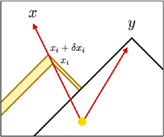
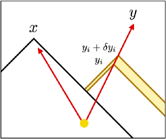
Refer to caption
Refer to caption
Refer to caption
Figure 21: (Top-left) CU𝐶𝑈CU contribution. The x𝑥x-fragment is intercepted in the time interval [tx,tx+dtx]subscript𝑡𝑥subscript𝑡𝑥𝑑subscript𝑡𝑥[t_{x},t_{x}+dt_{x}] by some bubble which does not intercept the y𝑦y-fragment before tysubscript𝑡𝑦t_{y}. Such a bubble nucleates in the thin yellow band. Note that the red arrows are on the past v𝑣v-cones of x𝑥x and y𝑦y, and their inclinations do not mean that bubble walls propagate slower than v𝑣v: see Fig. 13. (Top-right) UC𝑈𝐶UC contribution. Same as the top-left, except that the roles of x𝑥x and y𝑦y are interchanged. (Bottom) CC𝐶𝐶CC contribution. This contains two cases: one is that one bubble nucleates in each of the left and right thin yellow bands, and the other is that only one bubble nucleates in the small yellow diamond in the center.

C.2 Double-bubble simplification formula

(U,Ci)×(U,Ci)𝑈subscript𝐶𝑖𝑈subscript𝐶𝑖(U,C_{i})\times(U,C_{i}) contributions

Let us start from Eq. (B.6), which is written here again for completeness

Tij(x)Tkl(y)(d,UU)superscriptdelimited-⟨⟩subscript𝑇𝑖𝑗𝑥subscript𝑇𝑘𝑙𝑦𝑑𝑈𝑈\displaystyle\left<T_{ij}(x)T_{kl}(y)\right>^{(d,UU)} =tx𝑑txnty𝑑tyn𝑑Ωxn𝑑Ωynabsentsuperscriptsubscriptsubscript𝑡𝑥differential-dsubscript𝑡𝑥𝑛superscriptsubscriptsubscript𝑡𝑦differential-dsubscript𝑡𝑦𝑛differential-dsubscriptΩ𝑥𝑛differential-dsubscriptΩ𝑦𝑛\displaystyle=\int_{-\infty}^{t_{x}}dt_{xn}\int_{-\infty}^{t_{y}}dt_{yn}\int d\Omega_{xn}\int d\Omega_{yn}\;
Θsp(x,yn)Θsp(xn,y)eI(x,y)(d)(x,y;xi=x,yi=y;xn,yn).\displaystyle\;\;\;\;\Theta_{\rm sp}(x,y_{n})\Theta_{\rm sp}(x_{n},y)e^{-I(x,y)}{\mathcal{F}}^{(d)}(x,y;x_{i}=x,y_{i}=y;x_{n},y_{n}). (C.4)

Below we first show that the other contributions in (U,Ci)×(U,Ci)𝑈subscript𝐶𝑖𝑈subscript𝐶𝑖(U,C_{i})\times(U,C_{i}) are expressed as

Tij(x)Tkl(y)(d,UCi)superscriptdelimited-⟨⟩subscript𝑇𝑖𝑗𝑥subscript𝑇𝑘𝑙𝑦𝑑𝑈subscript𝐶𝑖\displaystyle\left<T_{ij}(x)T_{kl}(y)\right>^{(d,UC_{i})} =tx𝑑txnty𝑑tyntynty𝑑tyi𝑑Ωxn𝑑Ωynabsentsuperscriptsubscriptsubscript𝑡𝑥differential-dsubscript𝑡𝑥𝑛superscriptsubscriptsubscript𝑡𝑦differential-dsubscript𝑡𝑦𝑛superscriptsubscriptsubscript𝑡𝑦𝑛subscript𝑡𝑦differential-dsubscript𝑡𝑦𝑖differential-dsubscriptΩ𝑥𝑛differential-dsubscriptΩ𝑦𝑛\displaystyle=\int_{-\infty}^{t_{x}}dt_{xn}\int_{-\infty}^{t_{y}}dt_{yn}\int_{t_{yn}}^{t_{y}}dt_{yi}\int d\Omega_{xn}\int d\Omega_{yn}\;
Θsp(x,yn)Θsp(xn,yi)[I(x,yi)]tyieI(x,yi)(d)(x,y;xi=x,yi;xn,yn),\displaystyle\;\;\;\;\;\;\Theta_{\rm sp}(x,y_{n})\Theta_{\rm sp}(x_{n},y_{i})\left[I(x,y_{i})\right]_{tyi}e^{-I(x,y_{i})}{\mathcal{F}}^{(d)}(x,y;x_{i}=x,y_{i};x_{n},y_{n}),
Tij(x)Tkl(y)(d,CiU)superscriptdelimited-⟨⟩subscript𝑇𝑖𝑗𝑥subscript𝑇𝑘𝑙𝑦𝑑subscript𝐶𝑖𝑈\displaystyle\left<T_{ij}(x)T_{kl}(y)\right>^{(d,C_{i}U)} =tx𝑑txnty𝑑tyntxntx𝑑txi𝑑Ωxn𝑑Ωynabsentsuperscriptsubscriptsubscript𝑡𝑥differential-dsubscript𝑡𝑥𝑛superscriptsubscriptsubscript𝑡𝑦differential-dsubscript𝑡𝑦𝑛superscriptsubscriptsubscript𝑡𝑥𝑛subscript𝑡𝑥differential-dsubscript𝑡𝑥𝑖differential-dsubscriptΩ𝑥𝑛differential-dsubscriptΩ𝑦𝑛\displaystyle=\int_{-\infty}^{t_{x}}dt_{xn}\int_{-\infty}^{t_{y}}dt_{yn}\int_{t_{xn}}^{t_{x}}dt_{xi}\int d\Omega_{xn}\int d\Omega_{yn}\;
Θsp(xi,yn)Θsp(xn,y)[I(xi,y)]txieI(xi,y)(d)(x,y;xi,yi=y;xn,yn),\displaystyle\;\;\;\;\;\;\Theta_{\rm sp}(x_{i},y_{n})\Theta_{\rm sp}(x_{n},y)\left[I(x_{i},y)\right]_{txi}e^{-I(x_{i},y)}{\mathcal{F}}^{(d)}(x,y;x_{i},y_{i}=y;x_{n},y_{n}),
Tij(x)Tkl(y)(d,CiCi)superscriptdelimited-⟨⟩subscript𝑇𝑖𝑗𝑥subscript𝑇𝑘𝑙𝑦𝑑subscript𝐶𝑖subscript𝐶𝑖\displaystyle\left<T_{ij}(x)T_{kl}(y)\right>^{(d,C_{i}C_{i})} =tx𝑑txnty𝑑tyntxntx𝑑txitynty𝑑tyi𝑑Ωxn𝑑Ωynabsentsuperscriptsubscriptsubscript𝑡𝑥differential-dsubscript𝑡𝑥𝑛superscriptsubscriptsubscript𝑡𝑦differential-dsubscript𝑡𝑦𝑛superscriptsubscriptsubscript𝑡𝑥𝑛subscript𝑡𝑥differential-dsubscript𝑡𝑥𝑖superscriptsubscriptsubscript𝑡𝑦𝑛subscript𝑡𝑦differential-dsubscript𝑡𝑦𝑖differential-dsubscriptΩ𝑥𝑛differential-dsubscriptΩ𝑦𝑛\displaystyle=\int_{-\infty}^{t_{x}}dt_{xn}\int_{-\infty}^{t_{y}}dt_{yn}\int_{t_{xn}}^{t_{x}}dt_{xi}\int_{t_{yn}}^{t_{y}}dt_{yi}\int d\Omega_{xn}\int d\Omega_{yn}\;
Θsp(xi,yn)Θsp(xn,yi)[[I(xi,yi)]txi[I(xi,yi)]tyi[I(xi,yi)]txi,tyi]subscriptΘspsubscript𝑥𝑖subscript𝑦𝑛subscriptΘspsubscript𝑥𝑛subscript𝑦𝑖delimited-[]subscriptdelimited-[]𝐼subscript𝑥𝑖subscript𝑦𝑖𝑡𝑥𝑖subscriptdelimited-[]𝐼subscript𝑥𝑖subscript𝑦𝑖𝑡𝑦𝑖subscriptdelimited-[]𝐼subscript𝑥𝑖subscript𝑦𝑖𝑡𝑥𝑖𝑡𝑦𝑖\displaystyle\;\;\;\;\;\;\Theta_{\rm sp}(x_{i},y_{n})\Theta_{\rm sp}(x_{n},y_{i})\left[\left[I(x_{i},y_{i})\right]_{txi}\left[I(x_{i},y_{i})\right]_{tyi}-\left[I(x_{i},y_{i})\right]_{txi,tyi}\right]
eI(xi,yi)(d)(x,y;xi,yi;xn,yn).superscript𝑒𝐼subscript𝑥𝑖subscript𝑦𝑖superscript𝑑𝑥𝑦subscript𝑥𝑖subscript𝑦𝑖subscript𝑥𝑛subscript𝑦𝑛\displaystyle\;\;\;\;\;\;e^{-I(x_{i},y_{i})}{\mathcal{F}}^{(d)}(x,y;x_{i},y_{i};x_{n},y_{n}). (C.5)

Let us remember the arguments in Appendix B when we derive Eq. (C.4). The spacelike theta functions require (x,yn)𝑥subscript𝑦𝑛(x,y_{n}) and (xn,y)subscript𝑥𝑛𝑦(x_{n},y) to be spacelike. This is because, for timelike (x,yn)𝑥subscript𝑦𝑛(x,y_{n}) for example, either of the following two occurs:

  • For tx<tynsubscript𝑡𝑥subscript𝑡𝑦𝑛t_{x}<t_{yn}, ynsubscript𝑦𝑛y_{n} is in the future v𝑣v-cone of x𝑥x and therefore ynsubscript𝑦𝑛\vec{y}_{n} is already inside the x𝑥x-bubble at the nucleation time tynsubscript𝑡𝑦𝑛t_{yn}. This makes the nucleation of the y𝑦y-bubble impossible.

  • For tx>tynsubscript𝑡𝑥subscript𝑡𝑦𝑛t_{x}>t_{yn}, x𝑥x is in the future v𝑣v-cone of ynsubscript𝑦𝑛y_{n} and therefore x𝑥\vec{x} is already inside the y𝑦y-bubble at the evaluation time txsubscript𝑡𝑥t_{x}. This is not “U𝑈U” type contribution.

Therefore, the spacelike theta functions select out proper combinations of the nucleation points xnsubscript𝑥𝑛x_{n} and ynsubscript𝑦𝑛y_{n} for given x𝑥x and y𝑦y. Also, the false vacuum probability P(x,y)=eI(x,y)𝑃𝑥𝑦superscript𝑒𝐼𝑥𝑦P(x,y)=e^{-I(x,y)} guarantees that no bubbles nucleate in VxVysubscript𝑉𝑥subscript𝑉𝑦V_{x}\cup V_{y}, while the probability for bubble nucleation at proper spacetime points and the value of the energy-momentum tensor at the evaluation points are encoded in (d)superscript𝑑{\mathcal{F}}^{(d)}.

These arguments are modified in the other contributions in (U,Ci)×(U,Ci)𝑈subscript𝐶𝑖𝑈subscript𝐶𝑖(U,C_{i})\times(U,C_{i}). Let us take CiUsubscript𝐶𝑖𝑈C_{i}U as an example. See the left panel of Fig. 22. Now the x𝑥x-fragment has already been intercepted at the evaluation point txsubscript𝑡𝑥t_{x}, and therefore, in contrast to UU𝑈𝑈UU contribution, aaa we do not have to guarantee the “U𝑈U”(uncollided)-ness of the x𝑥x-fragment by Θsp(x,yn)subscriptΘsp𝑥subscript𝑦𝑛\Theta_{\rm sp}(x,y_{n}). Instead, Θsp(x,yn)subscriptΘsp𝑥subscript𝑦𝑛\Theta_{\rm sp}(x,y_{n}) must be replaced with Θsp(xi,yn)subscriptΘspsubscript𝑥𝑖subscript𝑦𝑛\Theta_{\rm sp}(x_{i},y_{n}). The reason is as follows. Even though the x𝑥x-fragment is allowed to collide with other bubbles before the evaluation time txsubscript𝑡𝑥t_{x}, it is not allowed before txisubscript𝑡𝑥𝑖t_{xi} because xisubscript𝑥𝑖x_{i} is the interception point, or the first collision point, by definition. Therefore we have to guarantee the “U𝑈U”-ness of the x𝑥x-fragment until the interception point xisubscript𝑥𝑖x_{i}, and that is why we replace Θsp(x,yn)subscriptΘsp𝑥subscript𝑦𝑛\Theta_{\rm sp}(x,y_{n}) with Θsp(xi,yn)subscriptΘspsubscript𝑥𝑖subscript𝑦𝑛\Theta_{\rm sp}(x_{i},y_{n}).♢♢\diamondsuit43♢♢\diamondsuit43\diamondsuit43 After this replacement, x𝑥x and ynsubscript𝑦𝑛y_{n} are no longer spacelike. One might worry that, if x𝑥x and ynsubscript𝑦𝑛y_{n} are timelike with tx<tynsubscript𝑡𝑥subscript𝑡𝑦𝑛t_{x}<t_{yn}, nucleation of the y𝑦y-bubble is not guaranteed because ynsubscript𝑦𝑛y_{n} is inside the future v𝑣v-cone of x𝑥x, which is inside the future v𝑣v-cone of xnsubscript𝑥𝑛x_{n} (that is, ynsubscript𝑦𝑛\vec{y}_{n} has already been past by the x𝑥x-bubble at the nucleation time tynsubscript𝑡𝑦𝑛t_{yn}). However, this never occurs. If ynsubscript𝑦𝑛y_{n} is inside the future v𝑣v-cone of x𝑥x, it means that ynsubscript𝑦𝑛y_{n} is also inside the future v𝑣v-cone of xisubscript𝑥𝑖x_{i} because the latter v𝑣v-cone contains the former. Such a combination of xisubscript𝑥𝑖x_{i} and ynsubscript𝑦𝑛y_{n} is forbidden by Θsp(xi,yn)subscriptΘspsubscript𝑥𝑖subscript𝑦𝑛\Theta_{\rm sp}(x_{i},y_{n}). On the other hand, the other spacelike theta function Θsp(xn,y)subscriptΘspsubscript𝑥𝑛𝑦\Theta_{\rm sp}(x_{n},y) remains the same, because otherwise the “U𝑈U”-ness of the y𝑦y-fragment is not guaranteed. The derivation of the remaining part (i.e. [I(x,yi)]tyieI(x,yi)subscriptdelimited-[]𝐼𝑥subscript𝑦𝑖𝑡𝑦𝑖superscript𝑒𝐼𝑥subscript𝑦𝑖\left[I(x,y_{i})\right]_{tyi}e^{-I(x,y_{i})} and (d)superscript𝑑{\mathcal{F}}^{(d)}) is basically the same as the single-bubble simplification formula. Since the spacelike theta functions themselves do not guarantee that proper bubble configurations are realized, we have to impose the following in order to realize such bubble configurations:

  • No bubbles nucleate in the union of the past v𝑣v-cones of xisubscript𝑥𝑖x_{i} and y𝑦y.

  • The bubble which intercepts the x𝑥x-fragment nucleates somewhere on the past v𝑣v-cone of xisubscript𝑥𝑖x_{i}, and it does not intercept the y𝑦y-fragment before the evaluation time tysubscript𝑡𝑦t_{y}.

Just as the single-bubble simplification formula, these are simultaneously taken into account by considering P(xi+δxi,y)P(xi,y)=[I(xi,y)]txieI(xi,y)𝑃subscript𝑥𝑖𝛿subscript𝑥𝑖𝑦𝑃subscript𝑥𝑖𝑦subscriptdelimited-[]𝐼subscript𝑥𝑖𝑦𝑡𝑥𝑖superscript𝑒𝐼subscript𝑥𝑖𝑦P(x_{i}+\delta x_{i},y)-P(x_{i},y)=\left[I(x_{i},y)\right]_{txi}e^{-I(x_{i},y)} for the interception of the x𝑥x-fragment in the time interval [txi,txi+dtxi]subscript𝑡𝑥𝑖subscript𝑡𝑥𝑖𝑑subscript𝑡𝑥𝑖[t_{xi},t_{xi}+dt_{xi}]. For the (d)superscript𝑑{\mathcal{F}}^{(d)} function, we have only to use (d)(x,y;xi=x,yi;xn,yn){\mathcal{F}}^{(d)}(x,y;x_{i}=x,y_{i};x_{n},y_{n}) to replace the value of the energy-momentum tensor at the evaluation points. These considerations give the expression for CiUsubscript𝐶𝑖𝑈C_{i}U in Eq. (C.5). For the UCi𝑈subscript𝐶𝑖UC_{i} contribution, the same argument holds with the roles of xsubscript𝑥x_{\bullet} and ysubscript𝑦y_{\bullet} interchanged.

For the CiCisubscript𝐶𝑖subscript𝐶𝑖C_{i}C_{i} contributions there are two possibilities, just like CC𝐶𝐶CC in the single-bubble contribution (see the bottom panel of Fig. 22):

  • One bubble nucleates in Vxi+δxi(VxiVyi+δyi)subscript𝑉subscript𝑥𝑖𝛿subscript𝑥𝑖subscript𝑉subscript𝑥𝑖subscript𝑉subscript𝑦𝑖𝛿subscript𝑦𝑖V_{x_{i}+\delta x_{i}}-(V_{x_{i}}\cup V_{y_{i}+\delta y_{i}}), and another nucleates in Vyi+δyi(Vxi+xi+δxiVyi)subscript𝑉subscript𝑦𝑖𝛿subscript𝑦𝑖subscript𝑉subscript𝑥𝑖subscript𝑥𝑖𝛿subscript𝑥𝑖subscript𝑉subscript𝑦𝑖V_{y_{i}+\delta y_{i}}-(V_{x_{i}+x_{i}+\delta x_{i}}\cup V_{y_{i}}).

  • One bubble nucleates in the small spacetime region (Vxi+δxiVyi+δyiVxiVyi)(Vxi+δxiVxi)(Vyi+δyiVyi)subscript𝑉subscript𝑥𝑖𝛿subscript𝑥𝑖subscript𝑉subscript𝑦𝑖𝛿subscript𝑦𝑖subscript𝑉subscript𝑥𝑖subscript𝑉subscript𝑦𝑖subscript𝑉subscript𝑥𝑖𝛿subscript𝑥𝑖subscript𝑉subscript𝑥𝑖subscript𝑉subscript𝑦𝑖𝛿subscript𝑦𝑖subscript𝑉subscript𝑦𝑖(V_{x_{i}+\delta x_{i}}\cup V_{y_{i}+\delta y_{i}}-V_{x_{i}}\cup V_{y_{i}})-(V_{x_{i}+\delta x_{i}}-V_{x_{i}})-(V_{y_{i}+\delta y_{i}}-V_{y_{i}}).

The sum of these two probabilities gives [[I(xi,yi)]txi[I(xi,yi)]tyi[I(xi,yi)]txi,tyi]dtxidtyidelimited-[]subscriptdelimited-[]𝐼subscript𝑥𝑖subscript𝑦𝑖𝑡𝑥𝑖subscriptdelimited-[]𝐼subscript𝑥𝑖subscript𝑦𝑖𝑡𝑦𝑖subscriptdelimited-[]𝐼subscript𝑥𝑖subscript𝑦𝑖𝑡𝑥𝑖𝑡𝑦𝑖𝑑subscript𝑡𝑥𝑖𝑑subscript𝑡𝑦𝑖\left[\left[I(x_{i},y_{i})\right]_{txi}\left[I(x_{i},y_{i})\right]_{tyi}-\left[I(x_{i},y_{i})\right]_{txi,tyi}\right]dt_{xi}dt_{yi}. For the (d)superscript𝑑{\mathcal{F}}^{(d)} function, we use (d)(x,y;xi,yi;xn,yn)superscript𝑑𝑥𝑦subscript𝑥𝑖subscript𝑦𝑖subscript𝑥𝑛subscript𝑦𝑛{\mathcal{F}}^{(d)}(x,y;x_{i},y_{i};x_{n},y_{n}) to take both interceptions into account. This completes the proof of Eq. (C.5). Now, using integration by parts as in deriving Eq. (C.3), we have

Tij(x)Tkl(y)(d,UU+UCi+CiU+CiCi)superscriptdelimited-⟨⟩subscript𝑇𝑖𝑗𝑥subscript𝑇𝑘𝑙𝑦𝑑𝑈𝑈𝑈subscript𝐶𝑖subscript𝐶𝑖𝑈subscript𝐶𝑖subscript𝐶𝑖\displaystyle\left<T_{ij}(x)T_{kl}(y)\right>^{(d,UU+UC_{i}+C_{i}U+C_{i}C_{i})}
=tx𝑑txnty𝑑tyntxntx𝑑txitynty𝑑tyi𝑑Ωxn𝑑Ωynabsentsuperscriptsubscriptsubscript𝑡𝑥differential-dsubscript𝑡𝑥𝑛superscriptsubscriptsubscript𝑡𝑦differential-dsubscript𝑡𝑦𝑛superscriptsubscriptsubscript𝑡𝑥𝑛subscript𝑡𝑥differential-dsubscript𝑡𝑥𝑖superscriptsubscriptsubscript𝑡𝑦𝑛subscript𝑡𝑦differential-dsubscript𝑡𝑦𝑖differential-dsubscriptΩ𝑥𝑛differential-dsubscriptΩ𝑦𝑛\displaystyle\;\;\;\;\;\;=\int_{-\infty}^{t_{x}}dt_{xn}\int_{-\infty}^{t_{y}}dt_{yn}\int_{t_{xn}}^{t_{x}}dt_{xi}\int_{t_{yn}}^{t_{y}}dt_{yi}\int d\Omega_{xn}\int d\Omega_{yn}\;
eI(xi,yi)[Θsp(xi,yn)Θsp(xn,yi)(d)(x,y;xi,yi;xn,yn)]txi,tyi,superscript𝑒𝐼subscript𝑥𝑖subscript𝑦𝑖subscriptdelimited-[]subscriptΘspsubscript𝑥𝑖subscript𝑦𝑛subscriptΘspsubscript𝑥𝑛subscript𝑦𝑖superscript𝑑𝑥𝑦subscript𝑥𝑖subscript𝑦𝑖subscript𝑥𝑛subscript𝑦𝑛𝑡𝑥𝑖𝑡𝑦𝑖\displaystyle\;\;\;\;\;\;\;\;\;\;\;\;e^{-I(x_{i},y_{i})}\left[\Theta_{\rm sp}(x_{i},y_{n})\Theta_{\rm sp}(x_{n},y_{i}){\mathcal{F}}^{(d)}(x,y;x_{i},y_{i};x_{n},y_{n})\right]_{txi,tyi}, (C.6)

as the sum of the four contributions.

Below we see the behavior of the time derivatives acting on the spacelike theta functions in Eq. (C.6), because such terms partly cancel out with the other five contributions in (U,Ci,Cin)×(U,Ci,Cin)𝑈subscript𝐶𝑖subscript𝐶𝑖𝑛𝑈subscript𝐶𝑖subscript𝐶𝑖𝑛(U,C_{i},C_{in})\times(U,C_{i},C_{in}). In the following, for given x𝑥x and y𝑦y, we regard Eq. (C.6) as first fixing (txn,tyn)subscript𝑡𝑥𝑛subscript𝑡𝑦𝑛(t_{xn},t_{yn}) and (Ωxn,Ωyn)subscriptΩ𝑥𝑛subscriptΩ𝑦𝑛(\Omega_{xn},\Omega_{yn}) and then scanning (txi,tyi)subscript𝑡𝑥𝑖subscript𝑡𝑦𝑖(t_{xi},t_{yi}), which means that we scan (xi,yi)subscript𝑥𝑖subscript𝑦𝑖(x_{i},y_{i}) along the propagation lines of x𝑥x- and y𝑦y-fragments. Now, let us consider [Θsp(xi,yn)]txisubscriptdelimited-[]subscriptΘspsubscript𝑥𝑖subscript𝑦𝑛𝑡𝑥𝑖\left[\Theta_{\rm sp}(x_{i},y_{n})\right]_{txi} for example. From the definition of the subscript on the square bracket, we take the derivative by changing txisubscript𝑡𝑥𝑖t_{xi} in Θsp(xi,yn)subscriptΘspsubscript𝑥𝑖subscript𝑦𝑛\Theta_{\rm sp}(x_{i},y_{n}) along the propagation of the x𝑥x-fragment. This derivative is nonzero only when the spacetime relation between (xi,yn)subscript𝑥𝑖subscript𝑦𝑛(x_{i},y_{n}) changes from timelike to spacelike (ΘspsubscriptΘsp\Theta_{\rm sp} changes from 00 to 111) or spacelike to timelike (ΘspsubscriptΘsp\Theta_{\rm sp} changes from 111 to 00). Such a spacetime point is either

  • On the past v𝑣v-cone of ynsubscript𝑦𝑛y_{n}.

  • On the future v𝑣v-cone of ynsubscript𝑦𝑛y_{n}.

We denote these points by xin(past)superscriptsubscript𝑥𝑖𝑛pastx_{in}^{\rm(past)} and xin(future)superscriptsubscript𝑥𝑖𝑛futurex_{in}^{\rm(future)}, respectively. See Fig. 23 for illustration. Though in this figure both xin(past)superscriptsubscript𝑥𝑖𝑛pastx_{in}^{\rm(past)} and xin(future)superscriptsubscript𝑥𝑖𝑛futurex_{in}^{\rm(future)} seem to exist, this is an artifact arising from plotting in two-dimensions. In fact, after some consideration, one sees that there is only one such point along the propagation line of the x𝑥x-fragment for given evaluation points (x,y)𝑥𝑦(x,y) and propagation directions (Ωxn,Ωyn).subscriptΩ𝑥𝑛subscriptΩ𝑦𝑛(\Omega_{xn},\Omega_{yn}).♢♢\diamondsuit44♢♢\diamondsuit44\diamondsuit44 In fact, the spacetime crossing point between the propagation line of the x𝑥x-fragment and both the past and future v𝑣v-cones of ynsubscript𝑦𝑛y_{n} can be calculated by squaring the identity xinyn=(xinx)(ynx)subscript𝑥𝑖𝑛subscript𝑦𝑛subscript𝑥𝑖𝑛𝑥subscript𝑦𝑛𝑥\vec{x}_{in}-\vec{y}_{n}=(\vec{x}_{in}-\vec{x})-(\vec{y}_{n}-\vec{x}) with |xinyn|=v|txin,yn|subscript𝑥𝑖𝑛subscript𝑦𝑛𝑣subscript𝑡𝑥𝑖𝑛𝑦𝑛|\vec{x}_{in}-\vec{y}_{n}|=v|t_{xin,yn}|, xinx=vtx,xinnxsubscript𝑥𝑖𝑛𝑥𝑣subscript𝑡𝑥𝑥𝑖𝑛subscript𝑛𝑥\vec{x}_{in}-\vec{x}=-vt_{x,xin}n_{x} and ynx=r+vty,ynnysubscript𝑦𝑛𝑥𝑟𝑣subscript𝑡𝑦𝑦𝑛subscript𝑛𝑦\vec{y}_{n}-\vec{x}=-\vec{r}+vt_{y,yn}n_{y}. Also, the crossing point between the propagation line of the y𝑦y-fragment and the past and future v𝑣v-cones of xnsubscript𝑥𝑛x_{n} is obtained by squaring yinxn=(yiny)(xny)subscript𝑦𝑖𝑛subscript𝑥𝑛subscript𝑦𝑖𝑛𝑦subscript𝑥𝑛𝑦\vec{y}_{in}-\vec{x}_{n}=(\vec{y}_{in}-\vec{y})-(\vec{x}_{n}-\vec{y}) with |yinxn|=v|tyin,xn|subscript𝑦𝑖𝑛subscript𝑥𝑛𝑣subscript𝑡𝑦𝑖𝑛𝑥𝑛|\vec{y}_{in}-\vec{x}_{n}|=v|t_{yin,xn}|, yiny=vty,yinnysubscript𝑦𝑖𝑛𝑦𝑣subscript𝑡𝑦𝑦𝑖𝑛subscript𝑛𝑦\vec{y}_{in}-\vec{y}=-vt_{y,yin}n_{y} and xny=r+vtxn,xnxsubscript𝑥𝑛𝑦𝑟𝑣subscript𝑡𝑥𝑛𝑥subscript𝑛𝑥\vec{x}_{n}-\vec{y}=\vec{r}+vt_{xn,x}n_{x}. The resulting expressions are txin,xsubscript𝑡𝑥𝑖𝑛𝑥\displaystyle t_{xin,x} =tx,yn2+ty,yn2+r22ty,ynrcy2(tx,yn+rcxty,yncxy),tyin,y=ty,xn2+tx,xn2+r2+2tx,xnrcx2(ty,xnrcytx,xncxy).formulae-sequenceabsentsuperscriptsubscript𝑡𝑥𝑦𝑛2superscriptsubscript𝑡𝑦𝑦𝑛2superscript𝑟22subscript𝑡𝑦𝑦𝑛𝑟subscript𝑐𝑦2subscript𝑡𝑥𝑦𝑛𝑟subscript𝑐𝑥subscript𝑡𝑦𝑦𝑛subscript𝑐𝑥𝑦subscript𝑡𝑦𝑖𝑛𝑦superscriptsubscript𝑡𝑦𝑥𝑛2superscriptsubscript𝑡𝑥𝑥𝑛2superscript𝑟22subscript𝑡𝑥𝑥𝑛𝑟subscript𝑐𝑥2subscript𝑡𝑦𝑥𝑛𝑟subscript𝑐𝑦subscript𝑡𝑥𝑥𝑛subscript𝑐𝑥𝑦\displaystyle=\frac{-t_{x,yn}^{2}+t_{y,yn}^{2}+r^{2}-2t_{y,yn}rc_{y}}{2(t_{x,yn}+rc_{x}-t_{y,yn}c_{xy})},\;\;\;\;t_{yin,y}=\frac{-t_{y,xn}^{2}+t_{x,xn}^{2}+r^{2}+2t_{x,xn}rc_{x}}{2(t_{y,xn}-rc_{y}-t_{x,xn}c_{xy})}. (C.7) Here cxy=nxnysubscript𝑐𝑥𝑦subscript𝑛𝑥subscript𝑛𝑦c_{xy}=n_{x}\cdot n_{y} is the cosine between the propagation angles of x𝑥x- and y𝑦y-fragments, and also we have presented these crossing points in terms of time differences txin,x=txintxsubscript𝑡𝑥𝑖𝑛𝑥subscript𝑡𝑥𝑖𝑛subscript𝑡𝑥t_{xin,x}=t_{xin}-t_{x} and tyin,y=tyintysubscript𝑡𝑦𝑖𝑛𝑦subscript𝑡𝑦𝑖𝑛subscript𝑡𝑦t_{yin,y}=t_{yin}-t_{y}. This means that there is a unique spacetime crossing point between the propagation line and the v𝑣v-cones. ♢♢\diamondsuit45♢♢\diamondsuit45\diamondsuit45 For special propagation directions with which the denominator of txin,xsubscript𝑡𝑥𝑖𝑛𝑥t_{xin,x} or tyin,ysubscript𝑡𝑦𝑖𝑛𝑦t_{yin,y} in Eq. (C.7) vanishes, there is no spacetime crossing between the propagation line and the v𝑣v-cone. Also, if the numerator vanishes in addition, there are infinite number of the crossing points. However, since such contributions occupy a vanishing measure in the integration, we can safely neglect them. After further consideration, one sees that only the future crossing point can appear in the integration region for txisubscript𝑡𝑥𝑖t_{xi}, and the past crossing point never appears in the integration.♢♢\diamondsuit46♢♢\diamondsuit46\diamondsuit46 The past crossing point does not appear in the integration region for the following reason. Suppose that it appears. Then, denoting the past crossing point by xinsubscript𝑥𝑖𝑛x_{in} for brevity, one finds that (xn,xin)subscript𝑥𝑛subscript𝑥𝑖𝑛(x_{n},x_{in}) is null with txn<txinsubscript𝑡𝑥𝑛subscript𝑡𝑥𝑖𝑛t_{xn}<t_{xin}. Also one finds that (xin,yn)subscript𝑥𝑖𝑛subscript𝑦𝑛(x_{in},y_{n}) is null with txin<tynsubscript𝑡𝑥𝑖𝑛subscript𝑡𝑦𝑛t_{xin}<t_{yn},      (yn,yi)subscript𝑦𝑛subscript𝑦𝑖(y_{n},y_{i}) is null with tyn<tyisubscript𝑡𝑦𝑛subscript𝑡𝑦𝑖t_{yn}<t_{yi}. Spacetime points xnsubscript𝑥𝑛x_{n} and yisubscript𝑦𝑖y_{i} satisfying these three conditions are timelike (except for limited cases with vanishing integration measure). Therefore the other spacelike theta function Θsp(xn,yi)subscriptΘspsubscript𝑥𝑛subscript𝑦𝑖\Theta_{\rm sp}(x_{n},y_{i}) in Eq. (C.6) vanishes. Therefore we write xin(future)superscriptsubscript𝑥𝑖𝑛futurex_{in}^{\rm(future)} simply as xinsubscript𝑥𝑖𝑛x_{in}, and take only this into account. The future crossing point between the propagation line of the y𝑦y-fragment and the v𝑣v-cones of xnsubscript𝑥𝑛x_{n} is defined in the same way, and we call it yinsubscript𝑦𝑖𝑛y_{in}. Now the time derivatives give

[Θsp(xi,yn)]txisubscriptdelimited-[]subscriptΘspsubscript𝑥𝑖subscript𝑦𝑛𝑡𝑥𝑖\displaystyle\left[\Theta_{\rm sp}(x_{i},y_{n})\right]_{txi} =δ(txitxin),[Θsp(xn,yi)]tyi=δ(tyityin),formulae-sequenceabsent𝛿subscript𝑡𝑥𝑖subscript𝑡𝑥𝑖𝑛subscriptdelimited-[]subscriptΘspsubscript𝑥𝑛subscript𝑦𝑖𝑡𝑦𝑖𝛿subscript𝑡𝑦𝑖subscript𝑡𝑦𝑖𝑛\displaystyle=-\delta(t_{xi}-t_{xin}),\;\;\;\;\left[\Theta_{\rm sp}(x_{n},y_{i})\right]_{tyi}=-\delta(t_{yi}-t_{yin}), (C.8)

where the minus signs arise because ΘspsubscriptΘsp\Theta_{\rm sp} changes from 111 to 00 at the future crossing points. Therefore, we can rewrite Eq. (C.6) as

Tij(x)Tkl(y)(d,UU+UCi+CiU+CiCi)superscriptdelimited-⟨⟩subscript𝑇𝑖𝑗𝑥subscript𝑇𝑘𝑙𝑦𝑑𝑈𝑈𝑈subscript𝐶𝑖subscript𝐶𝑖𝑈subscript𝐶𝑖subscript𝐶𝑖\displaystyle\left<T_{ij}(x)T_{kl}(y)\right>^{(d,UU+UC_{i}+C_{i}U+C_{i}C_{i})}
=tx𝑑txnty𝑑tyntxntx𝑑txitynty𝑑tyi𝑑Ωxn𝑑Ωynabsentsuperscriptsubscriptsubscript𝑡𝑥differential-dsubscript𝑡𝑥𝑛superscriptsubscriptsubscript𝑡𝑦differential-dsubscript𝑡𝑦𝑛superscriptsubscriptsubscript𝑡𝑥𝑛subscript𝑡𝑥differential-dsubscript𝑡𝑥𝑖superscriptsubscriptsubscript𝑡𝑦𝑛subscript𝑡𝑦differential-dsubscript𝑡𝑦𝑖differential-dsubscriptΩ𝑥𝑛differential-dsubscriptΩ𝑦𝑛\displaystyle\;\;\;\;\;\;=\int_{-\infty}^{t_{x}}dt_{xn}\int_{-\infty}^{t_{y}}dt_{yn}\int_{t_{xn}}^{t_{x}}dt_{xi}\int_{t_{yn}}^{t_{y}}dt_{yi}\int d\Omega_{xn}\int d\Omega_{yn}\;
eI(xi,yi)[δ(txitxin)δ(tyityin)(d)(x,y;xi,yi,xn,yn)δ(txitxin)Θsp(xn,yi)[(d)(x,y;xi,yi,xn,yn)]tyiΘsp(xi,yn)δ(tyityin)[(d)(x,y;xi,yi,xn,yn)]txi+Θsp(xi,yn)Θsp(xn,yi)[(d)(x,y;xi,yi,xn,yn)]txi,tyi].superscript𝑒𝐼subscript𝑥𝑖subscript𝑦𝑖delimited-[]matrix𝛿subscript𝑡𝑥𝑖subscript𝑡𝑥𝑖𝑛𝛿subscript𝑡𝑦𝑖subscript𝑡𝑦𝑖𝑛superscript𝑑𝑥𝑦subscript𝑥𝑖subscript𝑦𝑖subscript𝑥𝑛subscript𝑦𝑛𝛿subscript𝑡𝑥𝑖subscript𝑡𝑥𝑖𝑛subscriptΘspsubscript𝑥𝑛subscript𝑦𝑖subscriptdelimited-[]superscript𝑑𝑥𝑦subscript𝑥𝑖subscript𝑦𝑖subscript𝑥𝑛subscript𝑦𝑛𝑡𝑦𝑖subscriptΘspsubscript𝑥𝑖subscript𝑦𝑛𝛿subscript𝑡𝑦𝑖subscript𝑡𝑦𝑖𝑛subscriptdelimited-[]superscript𝑑𝑥𝑦subscript𝑥𝑖subscript𝑦𝑖subscript𝑥𝑛subscript𝑦𝑛𝑡𝑥𝑖subscriptΘspsubscript𝑥𝑖subscript𝑦𝑛subscriptΘspsubscript𝑥𝑛subscript𝑦𝑖subscriptdelimited-[]superscript𝑑𝑥𝑦subscript𝑥𝑖subscript𝑦𝑖subscript𝑥𝑛subscript𝑦𝑛𝑡𝑥𝑖𝑡𝑦𝑖\displaystyle\;\;\;\;\;\;\;\;\;\;\;\;e^{-I(x_{i},y_{i})}\left[\begin{matrix}[l]\;\delta(t_{xi}-t_{xin})\delta(t_{yi}-t_{yin}){\mathcal{F}}^{(d)}(x,y;x_{i},y_{i},x_{n},y_{n})\\[6.45831pt] -\;\delta(t_{xi}-t_{xin})\Theta_{\rm sp}(x_{n},y_{i})\left[{\mathcal{F}}^{(d)}(x,y;x_{i},y_{i},x_{n},y_{n})\right]_{tyi}\\[6.45831pt] -\;\Theta_{\rm sp}(x_{i},y_{n})\delta(t_{yi}-t_{yin})\left[{\mathcal{F}}^{(d)}(x,y;x_{i},y_{i},x_{n},y_{n})\right]_{txi}\\[6.45831pt] +\;\Theta_{\rm sp}(x_{i},y_{n})\Theta_{\rm sp}(x_{n},y_{i})\left[{\mathcal{F}}^{(d)}(x,y;x_{i},y_{i},x_{n},y_{n})\right]_{txi,tyi}\end{matrix}\right]. (C.9)

Below we see some of these terms cancel out with the other five contributions to give a simple formula.
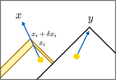
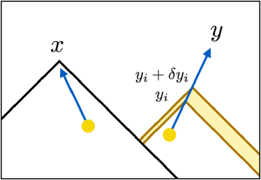
Refer to caption
Refer to caption
Refer to caption
Figure 22: (Top-left) CiUsubscript𝐶𝑖𝑈C_{i}U contribution. The x𝑥x-fragment is intercepted in the time interval [tx,tx+dtx]subscript𝑡𝑥subscript𝑡𝑥𝑑subscript𝑡𝑥[t_{x},t_{x}+dt_{x}] by some bubble which do not intercept the y𝑦y-fragment before tysubscript𝑡𝑦t_{y}. (Top-right) UCi𝑈subscript𝐶𝑖UC_{i} contribution. Same as the left panel, except that the role of x𝑥x and y𝑦y are interchanged. (Bottom) CiCisubscript𝐶𝑖subscript𝐶𝑖C_{i}C_{i} contribution. One possibility is that one bubble nucleates in each of the left and right thin yellow region, and the other possibility is that only one bubble nucleates in the small diamond-shaped region.
Refer to caption
Refer to caption
Figure 23: Definition of xin(past)superscriptsubscript𝑥𝑖𝑛pastx_{in}^{\rm(past)}, xin(future)superscriptsubscript𝑥𝑖𝑛futurex_{in}^{\rm(future)} (left) and yin(past)superscriptsubscript𝑦𝑖𝑛pasty_{in}^{\rm(past)}, yin(future)superscriptsubscript𝑦𝑖𝑛futurey_{in}^{\rm(future)} (right). They are the spacetime crossing points of the propagation line of the x𝑥x-(y𝑦y-)fragment and the v𝑣v-cones of ynsubscript𝑦𝑛y_{n} (xnsubscript𝑥𝑛x_{n}). If the crossing point is on the past (future) v𝑣v-cone, we label it with past (future). The derivative of the spacelike theta function [Θsp(xi,yn)]txisubscriptdelimited-[]subscriptΘspsubscript𝑥𝑖subscript𝑦𝑛𝑡𝑥𝑖\left[\Theta_{\rm sp}(x_{i},y_{n})\right]_{txi} or [Θsp(xn,yi)]tyisubscriptdelimited-[]subscriptΘspsubscript𝑥𝑛subscript𝑦𝑖𝑡𝑦𝑖\left[\Theta_{\rm sp}(x_{n},y_{i})\right]_{tyi} is nonzero only at these points. Note that there is only either of xin(past)superscriptsubscript𝑥𝑖𝑛pastx_{in}^{\rm(past)} or xin(future)superscriptsubscript𝑥𝑖𝑛futurex_{in}^{\rm(future)} (yin(past)superscriptsubscript𝑦𝑖𝑛pasty_{in}^{\rm(past)} or yin(future)superscriptsubscript𝑦𝑖𝑛futurey_{in}^{\rm(future)}). See the main text on this point.

(U,Ci,Cin)×(U,Ci,Cin)𝑈subscript𝐶𝑖subscript𝐶𝑖𝑛𝑈subscript𝐶𝑖subscript𝐶𝑖𝑛(U,C_{i},C_{in})\times(U,C_{i},C_{in}) contributions

Let us see the other five contributions, UCin𝑈subscript𝐶𝑖𝑛UC_{in}, CinUsubscript𝐶𝑖𝑛𝑈C_{in}U, CiCinsubscript𝐶𝑖subscript𝐶𝑖𝑛C_{i}C_{in}, CinCisubscript𝐶𝑖𝑛subscript𝐶𝑖C_{in}C_{i} and CinCinsubscript𝐶𝑖𝑛subscript𝐶𝑖𝑛C_{in}C_{in}. Remember that Cinsubscript𝐶𝑖𝑛C_{in} refers to those contributions where the x𝑥x-(or y𝑦y-)fragment is intercepted by the y𝑦y-(or x𝑥x-)bubble. Therefore, whether such a contribution exists or not depends on whether the future crossing point txinsubscript𝑡𝑥𝑖𝑛t_{xin} or tyinsubscript𝑡𝑦𝑖𝑛t_{yin} lies in the integration region [txn,tx]subscript𝑡𝑥𝑛subscript𝑡𝑥[t_{xn},t_{x}] or [tyn,ty]subscript𝑡𝑦𝑛subscript𝑡𝑦[t_{yn},t_{y}], respectively. However, in any cases, the five contributions can be written as follows:

Tij(x)Tkl(y)(d,UCin)=superscriptdelimited-⟨⟩subscript𝑇𝑖𝑗𝑥subscript𝑇𝑘𝑙𝑦𝑑𝑈subscript𝐶𝑖𝑛absent\displaystyle\left<T_{ij}(x)T_{kl}(y)\right>^{(d,UC_{in})}= tx𝑑txnty𝑑tyntynty𝑑tyi𝑑Ωxn𝑑Ωynsuperscriptsubscriptsubscript𝑡𝑥differential-dsubscript𝑡𝑥𝑛superscriptsubscriptsubscript𝑡𝑦differential-dsubscript𝑡𝑦𝑛superscriptsubscriptsubscript𝑡𝑦𝑛subscript𝑡𝑦differential-dsubscript𝑡𝑦𝑖differential-dsubscriptΩ𝑥𝑛differential-dsubscriptΩ𝑦𝑛\displaystyle\int_{-\infty}^{t_{x}}dt_{xn}\int_{-\infty}^{t_{y}}dt_{yn}\int_{t_{yn}}^{t_{y}}dt_{yi}\int d\Omega_{xn}\int d\Omega_{yn}\;
Θsp(x,yn)δ(tyityin)eI(x,yi)(d)(x,y;x,yi;xn,yn),subscriptΘsp𝑥subscript𝑦𝑛𝛿subscript𝑡𝑦𝑖subscript𝑡𝑦𝑖𝑛superscript𝑒𝐼𝑥subscript𝑦𝑖superscript𝑑𝑥𝑦𝑥subscript𝑦𝑖subscript𝑥𝑛subscript𝑦𝑛\displaystyle\Theta_{\rm sp}(x,y_{n})\delta(t_{yi}-t_{yin})e^{-I(x,y_{i})}{\mathcal{F}}^{(d)}(x,y;x,y_{i};x_{n},y_{n}), (C.10)
Tij(x)Tkl(y)(d,CinU)=superscriptdelimited-⟨⟩subscript𝑇𝑖𝑗𝑥subscript𝑇𝑘𝑙𝑦𝑑subscript𝐶𝑖𝑛𝑈absent\displaystyle\left<T_{ij}(x)T_{kl}(y)\right>^{(d,C_{in}U)}= tx𝑑txnty𝑑tyntxntx𝑑txi𝑑Ωxn𝑑Ωynsuperscriptsubscriptsubscript𝑡𝑥differential-dsubscript𝑡𝑥𝑛superscriptsubscriptsubscript𝑡𝑦differential-dsubscript𝑡𝑦𝑛superscriptsubscriptsubscript𝑡𝑥𝑛subscript𝑡𝑥differential-dsubscript𝑡𝑥𝑖differential-dsubscriptΩ𝑥𝑛differential-dsubscriptΩ𝑦𝑛\displaystyle\int_{-\infty}^{t_{x}}dt_{xn}\int_{-\infty}^{t_{y}}dt_{yn}\int_{t_{xn}}^{t_{x}}dt_{xi}\int d\Omega_{xn}\int d\Omega_{yn}\;
δ(txitxin)Θsp(xn,y)eI(xi,y)(d)(x,y;xi,y;xn,yn),𝛿subscript𝑡𝑥𝑖subscript𝑡𝑥𝑖𝑛subscriptΘspsubscript𝑥𝑛𝑦superscript𝑒𝐼subscript𝑥𝑖𝑦superscript𝑑𝑥𝑦subscript𝑥𝑖𝑦subscript𝑥𝑛subscript𝑦𝑛\displaystyle\delta(t_{xi}-t_{xin})\Theta_{\rm sp}(x_{n},y)e^{-I(x_{i},y)}{\mathcal{F}}^{(d)}(x,y;x_{i},y;x_{n},y_{n}), (C.11)
Tij(x)Tkl(y)(d,CiCin)=superscriptdelimited-⟨⟩subscript𝑇𝑖𝑗𝑥subscript𝑇𝑘𝑙𝑦𝑑subscript𝐶𝑖subscript𝐶𝑖𝑛absent\displaystyle\left<T_{ij}(x)T_{kl}(y)\right>^{(d,C_{i}C_{in})}= tx𝑑txnty𝑑tyntxntx𝑑txitynty𝑑tyi𝑑Ωxn𝑑Ωynsuperscriptsubscriptsubscript𝑡𝑥differential-dsubscript𝑡𝑥𝑛superscriptsubscriptsubscript𝑡𝑦differential-dsubscript𝑡𝑦𝑛superscriptsubscriptsubscript𝑡𝑥𝑛subscript𝑡𝑥differential-dsubscript𝑡𝑥𝑖superscriptsubscriptsubscript𝑡𝑦𝑛subscript𝑡𝑦differential-dsubscript𝑡𝑦𝑖differential-dsubscriptΩ𝑥𝑛differential-dsubscriptΩ𝑦𝑛\displaystyle\int_{-\infty}^{t_{x}}dt_{xn}\int_{-\infty}^{t_{y}}dt_{yn}\int_{t_{xn}}^{t_{x}}dt_{xi}\int_{t_{yn}}^{t_{y}}dt_{yi}\int d\Omega_{xn}\int d\Omega_{yn}\;
Θsp(xi,yn)δ(tyityin)[I(xi,yi)]txieI(xi,yi)(d)(x,y;xi,yi;xn,yn),subscriptΘspsubscript𝑥𝑖subscript𝑦𝑛𝛿subscript𝑡𝑦𝑖subscript𝑡𝑦𝑖𝑛subscriptdelimited-[]𝐼subscript𝑥𝑖subscript𝑦𝑖𝑡𝑥𝑖superscript𝑒𝐼subscript𝑥𝑖subscript𝑦𝑖superscript𝑑𝑥𝑦subscript𝑥𝑖subscript𝑦𝑖subscript𝑥𝑛subscript𝑦𝑛\displaystyle\Theta_{\rm sp}(x_{i},y_{n})\delta(t_{yi}-t_{yin})\left[I(x_{i},y_{i})\right]_{txi}e^{-I(x_{i},y_{i})}{\mathcal{F}}^{(d)}(x,y;x_{i},y_{i};x_{n},y_{n}), (C.12)
Tij(x)Tkl(y)(d,CinCi)=superscriptdelimited-⟨⟩subscript𝑇𝑖𝑗𝑥subscript𝑇𝑘𝑙𝑦𝑑subscript𝐶𝑖𝑛subscript𝐶𝑖absent\displaystyle\left<T_{ij}(x)T_{kl}(y)\right>^{(d,C_{in}C_{i})}= tx𝑑txnty𝑑tyntxntx𝑑txitynty𝑑tyi𝑑Ωxn𝑑Ωynsuperscriptsubscriptsubscript𝑡𝑥differential-dsubscript𝑡𝑥𝑛superscriptsubscriptsubscript𝑡𝑦differential-dsubscript𝑡𝑦𝑛superscriptsubscriptsubscript𝑡𝑥𝑛subscript𝑡𝑥differential-dsubscript𝑡𝑥𝑖superscriptsubscriptsubscript𝑡𝑦𝑛subscript𝑡𝑦differential-dsubscript𝑡𝑦𝑖differential-dsubscriptΩ𝑥𝑛differential-dsubscriptΩ𝑦𝑛\displaystyle\int_{-\infty}^{t_{x}}dt_{xn}\int_{-\infty}^{t_{y}}dt_{yn}\int_{t_{xn}}^{t_{x}}dt_{xi}\int_{t_{yn}}^{t_{y}}dt_{yi}\int d\Omega_{xn}\int d\Omega_{yn}\;
δ(txitxin)Θsp(xn,yi)[I(xi,yi)]tyieI(xi,yi)(d)(x,y;xi,yi;xn,yn),𝛿subscript𝑡𝑥𝑖subscript𝑡𝑥𝑖𝑛subscriptΘspsubscript𝑥𝑛subscript𝑦𝑖subscriptdelimited-[]𝐼subscript𝑥𝑖subscript𝑦𝑖𝑡𝑦𝑖superscript𝑒𝐼subscript𝑥𝑖subscript𝑦𝑖superscript𝑑𝑥𝑦subscript𝑥𝑖subscript𝑦𝑖subscript𝑥𝑛subscript𝑦𝑛\displaystyle\delta(t_{xi}-t_{xin})\Theta_{\rm sp}(x_{n},y_{i})\left[I(x_{i},y_{i})\right]_{tyi}e^{-I(x_{i},y_{i})}{\mathcal{F}}^{(d)}(x,y;x_{i},y_{i};x_{n},y_{n}), (C.13)
Tij(x)Tkl(y)(d,CinCin)=superscriptdelimited-⟨⟩subscript𝑇𝑖𝑗𝑥subscript𝑇𝑘𝑙𝑦𝑑subscript𝐶𝑖𝑛subscript𝐶𝑖𝑛absent\displaystyle\left<T_{ij}(x)T_{kl}(y)\right>^{(d,C_{in}C_{in})}= tx𝑑txnty𝑑tyntxntx𝑑txitynty𝑑tyi𝑑Ωxn𝑑Ωynsuperscriptsubscriptsubscript𝑡𝑥differential-dsubscript𝑡𝑥𝑛superscriptsubscriptsubscript𝑡𝑦differential-dsubscript𝑡𝑦𝑛superscriptsubscriptsubscript𝑡𝑥𝑛subscript𝑡𝑥differential-dsubscript𝑡𝑥𝑖superscriptsubscriptsubscript𝑡𝑦𝑛subscript𝑡𝑦differential-dsubscript𝑡𝑦𝑖differential-dsubscriptΩ𝑥𝑛differential-dsubscriptΩ𝑦𝑛\displaystyle\int_{-\infty}^{t_{x}}dt_{xn}\int_{-\infty}^{t_{y}}dt_{yn}\int_{t_{xn}}^{t_{x}}dt_{xi}\int_{t_{yn}}^{t_{y}}dt_{yi}\int d\Omega_{xn}\int d\Omega_{yn}\;
δ(txitxin)δ(tyityin)eI(xi,yi)(d)(x,y;xi,yi;xn,yn).𝛿subscript𝑡𝑥𝑖subscript𝑡𝑥𝑖𝑛𝛿subscript𝑡𝑦𝑖subscript𝑡𝑦𝑖𝑛superscript𝑒𝐼subscript𝑥𝑖subscript𝑦𝑖superscript𝑑𝑥𝑦subscript𝑥𝑖subscript𝑦𝑖subscript𝑥𝑛subscript𝑦𝑛\displaystyle\delta(t_{xi}-t_{xin})\delta(t_{yi}-t_{yin})e^{-I(x_{i},y_{i})}{\mathcal{F}}^{(d)}(x,y;x_{i},y_{i};x_{n},y_{n}). (C.14)

First let us see the CinUsubscript𝐶𝑖𝑛𝑈C_{in}U contribution (C.11). When the future crossing point txinsubscript𝑡𝑥𝑖𝑛t_{xin} does not lie in the integration region [txn,tx]subscript𝑡𝑥𝑛subscript𝑡𝑥[t_{xn},t_{x}], this expression trivially holds since it vanishes. On the other hand, when txinsubscript𝑡𝑥𝑖𝑛t_{xin} lies in the integration region [txn,tx]subscript𝑡𝑥𝑛subscript𝑡𝑥[t_{xn},t_{x}], one can perform the txisubscript𝑡𝑥𝑖t_{xi} integration. This replaces all the xisubscript𝑥𝑖x_{i} in the integrand with xinsubscript𝑥𝑖𝑛x_{in}. Now the meanings of the factors in the integrand are clear: Θsp(xn,y)subscriptΘspsubscript𝑥𝑛𝑦\Theta_{\rm sp}(x_{n},y) guarantees the “U𝑈U”-ness of the y𝑦y-fragment. P(xin,y)=eI(xin,y)𝑃subscript𝑥𝑖𝑛𝑦superscript𝑒𝐼subscript𝑥𝑖𝑛𝑦P(x_{in},y)=e^{-I(x_{in},y)} guarantees that no bubbles nucleate in the union of the past v𝑣v-cones of xinsubscript𝑥𝑖𝑛x_{in} and y𝑦y, which is necessary for xinsubscript𝑥𝑖𝑛x_{in} to be the interception (first collision) point and for y𝑦y to remain uncollided until the evaluation time. (d)superscript𝑑{\mathcal{F}}^{(d)} with xisubscript𝑥𝑖x_{i} replaced by xinsubscript𝑥𝑖𝑛x_{in} represents the proper value of the energy-momentum tensor. Note that no spacelike theta function appears for xisubscript𝑥𝑖x_{i} and ynsubscript𝑦𝑛y_{n} because they are null with each other in the present case. The same arguments apply to UCin𝑈subscript𝐶𝑖𝑛UC_{in} contribution (C.10).

Next let us see the CinCisubscript𝐶𝑖𝑛subscript𝐶𝑖C_{in}C_{i} contribution (C.13). This trivially holds when txinsubscript𝑡𝑥𝑖𝑛t_{xin} does not lie in the integration region [txn,tx]subscript𝑡𝑥𝑛subscript𝑡𝑥[t_{xn},t_{x}]. In the opposite case, one can perform txisubscript𝑡𝑥𝑖t_{xi} integration to replace all the xisubscript𝑥𝑖x_{i} in the integrand with xinsubscript𝑥𝑖𝑛x_{in}. Now the meanings of the factors in the integrand are as follows: Θsp(xn,yi)subscriptΘspsubscript𝑥𝑛subscript𝑦𝑖\Theta_{\rm sp}(x_{n},y_{i}) guarantees that yisubscript𝑦𝑖y_{i} is the interception (first collision) point. [I(xin,yi)]tyieI(xin,yi)subscriptdelimited-[]𝐼subscript𝑥𝑖𝑛subscript𝑦𝑖𝑡𝑦𝑖superscript𝑒𝐼subscript𝑥𝑖𝑛subscript𝑦𝑖\left[I(x_{in},y_{i})\right]_{tyi}e^{-I(x_{in},y_{i})} guarantees that no bubbles nucleate in the union of the past v𝑣v-cones of xinsubscript𝑥𝑖𝑛x_{in} and yisubscript𝑦𝑖y_{i}, and also that the intercepting bubble for the y𝑦y-fragment nucleate somewhere on the past v𝑣v-cone of yisubscript𝑦𝑖y_{i} so that the interception occurs in the time interval [tyi,tyi+dtyi]subscript𝑡𝑦𝑖subscript𝑡𝑦𝑖𝑑subscript𝑡𝑦𝑖[t_{yi},t_{yi}+dt_{yi}]. (d)superscript𝑑{\mathcal{F}}^{(d)} with xisubscript𝑥𝑖x_{i} replaced by xinsubscript𝑥𝑖𝑛x_{in} represents the proper value of the energy-momentum tensor. The same arguments apply to CiCinsubscript𝐶𝑖subscript𝐶𝑖𝑛C_{i}C_{in} contribution (C.12).

The last is the CinCinsubscript𝐶𝑖𝑛subscript𝐶𝑖𝑛C_{in}C_{in} contribution (C.14). We consider those cases where both txinsubscript𝑡𝑥𝑖𝑛t_{xin} and tyinsubscript𝑡𝑦𝑖𝑛t_{yin} are in the integration regions since otherwise trivial. We can perform txisubscript𝑡𝑥𝑖t_{xi} and tyisubscript𝑡𝑦𝑖t_{yi} integrations, and the resulting false vacuum probability P(xin,yin)=eI(xin,yin)𝑃subscript𝑥𝑖𝑛subscript𝑦𝑖𝑛superscript𝑒𝐼subscript𝑥𝑖𝑛subscript𝑦𝑖𝑛P(x_{in},y_{in})=e^{-I(x_{in},y_{in})} guarantees that no bubbles nucleate in the union of the past v𝑣v-cones of xinsubscript𝑥𝑖𝑛x_{in} and yinsubscript𝑦𝑖𝑛y_{in}, while (d)superscript𝑑{\mathcal{F}}^{(d)} with (xi,yi)subscript𝑥𝑖subscript𝑦𝑖(x_{i},y_{i}) replaced by (xin,yin)subscript𝑥𝑖𝑛subscript𝑦𝑖𝑛(x_{in},y_{in}) properly represents the value of the energy-momentum tensor in the CinCinsubscript𝐶𝑖𝑛subscript𝐶𝑖𝑛C_{in}C_{in} contribution.

Finally, we sum up all the contributions (C.9)–(C.14). All the terms except for the last one in Eq. (C.9) cancel out to give♢♢\diamondsuit47♢♢\diamondsuit47\diamondsuit47 The procedure is as follows. Eq. (C.12) and the third line in the square bracket in Eq. (C.9) give a term like [eI(xi,yi)(d)]txisubscriptdelimited-[]superscript𝑒𝐼subscript𝑥𝑖subscript𝑦𝑖superscript𝑑𝑡𝑥𝑖\left[-e^{-I(x_{i},y_{i})}{\mathcal{F}}^{(d)}\right]_{txi}. Integration by parts with respect to txisubscript𝑡𝑥𝑖t_{xi} gives a surface term at txi=txsubscript𝑡𝑥𝑖subscript𝑡𝑥t_{xi}=t_{x} and a term with two δ𝛿\delta-functions. The former cancels out with Eq. (C.10). Similar procedure on Eq. (C.13) and the second line in Eq. (C.9) gives a surface term at tyi=tysubscript𝑡𝑦𝑖subscript𝑡𝑦t_{yi}=t_{y} and a term with two δ𝛿\delta-functions. The former cancels out with Eq. (C.11). The remaining term cancels out with the first line in Eq. (C.9) and Eq. (C.14). This leaves only the last line in Eq. (C.9).

Tij(x)Tkl(y)(d,(U,Ci,Cin)×(U,Ci,Cin))superscriptdelimited-⟨⟩subscript𝑇𝑖𝑗𝑥subscript𝑇𝑘𝑙𝑦𝑑𝑈subscript𝐶𝑖subscript𝐶𝑖𝑛𝑈subscript𝐶𝑖subscript𝐶𝑖𝑛\displaystyle\left<T_{ij}(x)T_{kl}(y)\right>^{(d,(U,C_{i},C_{in})\times(U,C_{i},C_{in}))}
=tx𝑑txnty𝑑tyntxntx𝑑txitynty𝑑tyi𝑑Ωxn𝑑Ωynabsentsuperscriptsubscriptsubscript𝑡𝑥differential-dsubscript𝑡𝑥𝑛superscriptsubscriptsubscript𝑡𝑦differential-dsubscript𝑡𝑦𝑛superscriptsubscriptsubscript𝑡𝑥𝑛subscript𝑡𝑥differential-dsubscript𝑡𝑥𝑖superscriptsubscriptsubscript𝑡𝑦𝑛subscript𝑡𝑦differential-dsubscript𝑡𝑦𝑖differential-dsubscriptΩ𝑥𝑛differential-dsubscriptΩ𝑦𝑛\displaystyle\;\;\;\;\;\;\;\;=\int_{-\infty}^{t_{x}}dt_{xn}\int_{-\infty}^{t_{y}}dt_{yn}\int_{t_{xn}}^{t_{x}}dt_{xi}\int_{t_{yn}}^{t_{y}}dt_{yi}\int d\Omega_{xn}\int d\Omega_{yn}\;
Θsp(xi,yn)Θsp(xn,yi)eI(xi,yi)[(d)(x,y;xi,yi;xn,yn)]txi,tyi.subscriptΘspsubscript𝑥𝑖subscript𝑦𝑛subscriptΘspsubscript𝑥𝑛subscript𝑦𝑖superscript𝑒𝐼subscript𝑥𝑖subscript𝑦𝑖subscriptdelimited-[]superscript𝑑𝑥𝑦subscript𝑥𝑖subscript𝑦𝑖subscript𝑥𝑛subscript𝑦𝑛𝑡𝑥𝑖𝑡𝑦𝑖\displaystyle\;\;\;\;\;\;\;\;\;\;\;\;\;\;\;\;\Theta_{\rm sp}(x_{i},y_{n})\Theta_{\rm sp}(x_{n},y_{i})e^{-I(x_{i},y_{i})}\left[{\mathcal{F}}^{(d)}(x,y;x_{i},y_{i};x_{n},y_{n})\right]_{txi,tyi}. (C.15)

This is what we call the “simplification formula” for the double-bubble.

Appendix D Techniques for numerical evaluation

In this appendix we explain several techniques used for numerical evaluation of the GW spectrum.

D.1 Equivalent ways to impose the spacelike conditions

In the double-bubble contribution (B.20), we encounter two spacelike theta functions. In this subsection, we show that they can be replaced by one spacelike theta function. This replacement makes it possible to integrate out tx,xnsubscript𝑡𝑥𝑥𝑛t_{x,xn} and ty,ynsubscript𝑡𝑦𝑦𝑛t_{y,yn} directions, and as a result leaves seven-dimensional integration.

First, we write Eq. (B.20) here again for completeness:

Δ(d)=superscriptΔ𝑑absent\displaystyle\Delta^{(d)}= 𝑑tx,y0𝑑rvsuperscriptsubscriptdifferential-dsubscript𝑡𝑥𝑦superscriptsubscript0differential-dsubscript𝑟𝑣\displaystyle\int_{-\infty}^{\infty}dt_{x,y}\int_{0}^{\infty}dr_{v}
0𝑑tx,xn0𝑑ty,yn0tx,xn𝑑tx,xi0ty,yn𝑑ty,yi11𝑑cxn11𝑑cyn02π𝑑ϕxn,ynsuperscriptsubscript0differential-dsubscript𝑡𝑥𝑥𝑛superscriptsubscript0differential-dsubscript𝑡𝑦𝑦𝑛superscriptsubscript0subscript𝑡𝑥𝑥𝑛differential-dsubscript𝑡𝑥𝑥𝑖superscriptsubscript0subscript𝑡𝑦𝑦𝑛differential-dsubscript𝑡𝑦𝑦𝑖superscriptsubscript11differential-dsubscript𝑐𝑥𝑛superscriptsubscript11differential-dsubscript𝑐𝑦𝑛superscriptsubscript02𝜋differential-dsubscriptitalic-ϕ𝑥𝑛𝑦𝑛\displaystyle\int_{0}^{\infty}dt_{x,xn}\int_{0}^{\infty}dt_{y,yn}\int_{0}^{t_{x,xn}}dt_{x,xi}\int_{0}^{t_{y,yn}}dt_{y,yi}\int_{-1}^{1}dc_{xn}\int_{-1}^{1}dc_{yn}\int_{0}^{2\pi}d\phi_{xn,yn}
v3k33superscript𝑣3superscript𝑘33\displaystyle\frac{v^{3}k^{3}}{3} [Θsp(xi,yn)Θsp(xn,yi)×e(txi,xn+tyi,yn)e(tx,xi+ty,yi)/τ(txi,yi,rxi,yi/v)2(3txi,xn2+txi,xn3/τ)(3tyi,yn2+tyi,yn3/τ)×rv2[j0(vkrv)𝒦0(nxn,nyn)+j1(vkrv)vkrv𝒦1(nxn,nyn)+j2(vkrv)(vkrv)2𝒦2(nxn,nyn)]×cos(ktx,y)].delimited-[]matrixsubscriptΘspsubscript𝑥𝑖subscript𝑦𝑛subscriptΘspsubscript𝑥𝑛subscript𝑦𝑖absentsuperscript𝑒subscript𝑡𝑥𝑖𝑥𝑛subscript𝑡𝑦𝑖𝑦𝑛superscript𝑒subscript𝑡𝑥𝑥𝑖subscript𝑡𝑦𝑦𝑖𝜏superscriptsubscript𝑡𝑥𝑖𝑦𝑖subscript𝑟𝑥𝑖𝑦𝑖𝑣23superscriptsubscript𝑡𝑥𝑖𝑥𝑛2superscriptsubscript𝑡𝑥𝑖𝑥𝑛3𝜏3superscriptsubscript𝑡𝑦𝑖𝑦𝑛2superscriptsubscript𝑡𝑦𝑖𝑦𝑛3𝜏absentsuperscriptsubscript𝑟𝑣2delimited-[]subscript𝑗0𝑣𝑘subscript𝑟𝑣subscript𝒦0subscript𝑛𝑥𝑛subscript𝑛𝑦𝑛subscript𝑗1𝑣𝑘subscript𝑟𝑣𝑣𝑘subscript𝑟𝑣subscript𝒦1subscript𝑛𝑥𝑛subscript𝑛𝑦𝑛subscript𝑗2𝑣𝑘subscript𝑟𝑣superscript𝑣𝑘subscript𝑟𝑣2subscript𝒦2subscript𝑛𝑥𝑛subscript𝑛𝑦𝑛absent𝑘subscript𝑡𝑥𝑦\displaystyle\left[\begin{matrix}[l]\;\Theta_{\rm sp}(x_{i},y_{n})\Theta_{\rm sp}(x_{n},y_{i})\\[6.45831pt] \displaystyle\times\;\frac{e^{-(t_{xi,xn}+t_{yi,yn})}e^{-(t_{x,xi}+t_{y,yi})/\tau}}{{\mathcal{I}}(t_{xi,yi},r_{xi,yi}/v)^{2}}(3t_{xi,xn}^{2}+t_{xi,xn}^{3}/\tau)(3t_{yi,yn}^{2}+t_{yi,yn}^{3}/\tau)\\[8.61108pt] \displaystyle\times\;r_{v}^{2}\left[j_{0}(vkr_{v}){\mathcal{K}}_{0}(n_{xn},n_{yn})+\frac{j_{1}(vkr_{v})}{vkr_{v}}{\mathcal{K}}_{1}(n_{xn},n_{yn})+\frac{j_{2}(vkr_{v})}{(vkr_{v})^{2}}{\mathcal{K}}_{2}(n_{xn},n_{yn})\right]\\[8.61108pt] \times\cos(kt_{x,y})\end{matrix}\right]. (D.1)

Suppose that we first fix the evaluation points (x,y)𝑥𝑦(x,y) and the propagation directions of the wall fragments (Ωxn,Ωyn)subscriptΩ𝑥𝑛subscriptΩ𝑦𝑛(\Omega_{xn},\Omega_{yn}). Then, the spacelike theta functions in this expression require two nucleation points (xn,yn)subscript𝑥𝑛subscript𝑦𝑛(x_{n},y_{n}) and two interception points (xi,yi)subscript𝑥𝑖subscript𝑦𝑖(x_{i},y_{i}) to satisfy

  • (xi,yn)subscript𝑥𝑖subscript𝑦𝑛(x_{i},y_{n}) are spacelike.

  • (xn,yi)subscript𝑥𝑛subscript𝑦𝑖(x_{n},y_{i}) are spacelike.

We illustrate this procedure in the left panel of Fig. 24. Fixing (x,y)𝑥𝑦(x,y) and (Ωxn,Ωyn)subscriptΩ𝑥𝑛subscriptΩ𝑦𝑛(\Omega_{xn},\Omega_{yn}) corresponds to fixing the separation and directions of the two blue lines in this figure. Then finding (xn,yn)subscript𝑥𝑛subscript𝑦𝑛(x_{n},y_{n}) and (xi,yi)subscript𝑥𝑖subscript𝑦𝑖(x_{i},y_{i}) satisfying the above conditions means finding four points on these lines so that (xi,yn)subscript𝑥𝑖subscript𝑦𝑛(x_{i},y_{n}) and (xn,yi)subscript𝑥𝑛subscript𝑦𝑖(x_{n},y_{i}) are spacelike (denoted by the green solid lines). Now we argue that this procedure is equivalent to the following

  • Find spacelike (xi,yi)subscript𝑥𝑖subscript𝑦𝑖(x_{i},y_{i}).

  • Fix (xn,yn)subscript𝑥𝑛subscript𝑦𝑛(x_{n},y_{n}) so that xnsubscript𝑥𝑛x_{n} lies between xnisubscript𝑥𝑛𝑖x_{ni} and xisubscript𝑥𝑖x_{i} and ynsubscript𝑦𝑛y_{n} lies between ynisubscript𝑦𝑛𝑖y_{ni} and yisubscript𝑦𝑖y_{i}.

Here xnisubscript𝑥𝑛𝑖x_{ni} and ynisubscript𝑦𝑛𝑖y_{ni} are defined as the spacetime crossing points between the propagation lines of the x𝑥x- and y𝑦y-fragments and the past v𝑣v-cone of yisubscript𝑦𝑖y_{i} and xisubscript𝑥𝑖x_{i}, respectively. We illustrate this procedure in the right panel of Fig. 24.

The equivalence is proven as follows. First, suppose that we have spacelike combinations of (xi,yn)subscript𝑥𝑖subscript𝑦𝑛(x_{i},y_{n}) and (xn,yi)subscript𝑥𝑛subscript𝑦𝑖(x_{n},y_{i}). Then (xi,yi)subscript𝑥𝑖subscript𝑦𝑖(x_{i},y_{i}) are spacelike because otherwise either of (xi,yn)subscript𝑥𝑖subscript𝑦𝑛(x_{i},y_{n}) or (xn,yi)subscript𝑥𝑛subscript𝑦𝑖(x_{n},y_{i}) becomes timelike (note that txn<txisubscript𝑡𝑥𝑛subscript𝑡𝑥𝑖t_{xn}<t_{xi} and tyn<tyisubscript𝑡𝑦𝑛subscript𝑡𝑦𝑖t_{yn}<t_{yi}). Also xnsubscript𝑥𝑛x_{n} (ynsubscript𝑦𝑛y_{n}) lies between xnisubscript𝑥𝑛𝑖x_{ni} and xisubscript𝑥𝑖x_{i} (ynisubscript𝑦𝑛𝑖y_{ni} and yisubscript𝑦𝑖y_{i}) because otherwise it enters the past v𝑣v-cone of yisubscript𝑦𝑖y_{i} (xisubscript𝑥𝑖x_{i}) and becomes timelike to yisubscript𝑦𝑖y_{i} (xisubscript𝑥𝑖x_{i}). Second, suppose that (xi,yi)subscript𝑥𝑖subscript𝑦𝑖(x_{i},y_{i}) are spacelike and that xnsubscript𝑥𝑛x_{n} (ynsubscript𝑦𝑛y_{n}) is chosen so that it is between xnisubscript𝑥𝑛𝑖x_{ni} and xnsubscript𝑥𝑛x_{n} (ynisubscript𝑦𝑛𝑖y_{ni} and ynsubscript𝑦𝑛y_{n}). Then (xi,yn)subscript𝑥𝑖subscript𝑦𝑛(x_{i},y_{n}) and (xn,yi)subscript𝑥𝑛subscript𝑦𝑖(x_{n},y_{i}) are spacelike combinations because xnsubscript𝑥𝑛x_{n} and ynsubscript𝑦𝑛y_{n} are outside the past v𝑣v-cone of yisubscript𝑦𝑖y_{i} and xisubscript𝑥𝑖x_{i}, respectively. This proves the equivalence.

Here one may notice that xnisubscript𝑥𝑛𝑖x_{ni} and ynisubscript𝑦𝑛𝑖y_{ni} do not necessarily exist, just as xinsubscript𝑥𝑖𝑛x_{in} and yinsubscript𝑦𝑖𝑛y_{in} do not necessarily exist in Appendix B.4. In fact, there is only one spacetime crossing point between the propagation line of the x𝑥x-(or y𝑦y-)fragment and the past and future v𝑣v-cones of yisubscript𝑦𝑖y_{i} (or xisubscript𝑥𝑖x_{i}). They are given by♢♢\diamondsuit48♢♢\diamondsuit48\diamondsuit48 These are obtained by squaring the identity xniyi=(xnix)(yix)subscript𝑥𝑛𝑖subscript𝑦𝑖subscript𝑥𝑛𝑖𝑥subscript𝑦𝑖𝑥\vec{x}_{ni}-\vec{y}_{i}=(\vec{x}_{ni}-\vec{x})-(\vec{y}_{i}-\vec{x}) with |xniyi|=v|txni,yi|subscript𝑥𝑛𝑖subscript𝑦𝑖𝑣subscript𝑡𝑥𝑛𝑖𝑦𝑖|\vec{x}_{ni}-\vec{y}_{i}|=v|t_{xni,yi}|, xnix=vtx,xninxsubscript𝑥𝑛𝑖𝑥𝑣subscript𝑡𝑥𝑥𝑛𝑖subscript𝑛𝑥\vec{x}_{ni}-\vec{x}=vt_{x,xni}n_{x} and yix=r+vty,yinysubscript𝑦𝑖𝑥𝑟𝑣subscript𝑡𝑦𝑦𝑖subscript𝑛𝑦\vec{y}_{i}-\vec{x}=-\vec{r}+vt_{y,yi}n_{y}, and the identity ynixi=(yniy)(xiy)subscript𝑦𝑛𝑖subscript𝑥𝑖subscript𝑦𝑛𝑖𝑦subscript𝑥𝑖𝑦\vec{y}_{ni}-\vec{x}_{i}=(\vec{y}_{ni}-\vec{y})-(\vec{x}_{i}-\vec{y}) with |ynixi|=v|tyni,xi|subscript𝑦𝑛𝑖subscript𝑥𝑖𝑣subscript𝑡𝑦𝑛𝑖𝑥𝑖|\vec{y}_{ni}-\vec{x}_{i}|=v|t_{yni,xi}|, yniy=vty,yninysubscript𝑦𝑛𝑖𝑦𝑣subscript𝑡𝑦𝑦𝑛𝑖subscript𝑛𝑦\vec{y}_{ni}-\vec{y}=vt_{y,yni}n_{y} and xiy=r+vtx,xinxsubscript𝑥𝑖𝑦𝑟𝑣subscript𝑡𝑥𝑥𝑖subscript𝑛𝑥\vec{x}_{i}-\vec{y}=\vec{r}+vt_{x,xi}n_{x}, respectively.

txni,xsubscript𝑡𝑥𝑛𝑖𝑥\displaystyle t_{xni,x} =tx,yi2+ty,yi2+r22ty,yircy2(tx,yi+rcxty,yicxy),tyni,y=ty,xi2+tx,xi2+r2+2tx,xircx2(ty,xircytx,xicxy).formulae-sequenceabsentsuperscriptsubscript𝑡𝑥𝑦𝑖2superscriptsubscript𝑡𝑦𝑦𝑖2superscript𝑟22subscript𝑡𝑦𝑦𝑖𝑟subscript𝑐𝑦2subscript𝑡𝑥𝑦𝑖𝑟subscript𝑐𝑥subscript𝑡𝑦𝑦𝑖subscript𝑐𝑥𝑦subscript𝑡𝑦𝑛𝑖𝑦superscriptsubscript𝑡𝑦𝑥𝑖2superscriptsubscript𝑡𝑥𝑥𝑖2superscript𝑟22subscript𝑡𝑥𝑥𝑖𝑟subscript𝑐𝑥2subscript𝑡𝑦𝑥𝑖𝑟subscript𝑐𝑦subscript𝑡𝑥𝑥𝑖subscript𝑐𝑥𝑦\displaystyle=\frac{-t_{x,yi}^{2}+t_{y,yi}^{2}+r^{2}-2t_{y,yi}rc_{y}}{2(t_{x,yi}+rc_{x}-t_{y,yi}c_{xy})},\;\;\;\;t_{yni,y}=\frac{-t_{y,xi}^{2}+t_{x,xi}^{2}+r^{2}+2t_{x,xi}rc_{x}}{2(t_{y,xi}-rc_{y}-t_{x,xi}c_{xy})}. (D.2)

Therefore the past crossing point xnisubscript𝑥𝑛𝑖x_{ni} or ynisubscript𝑦𝑛𝑖y_{ni} does not exist if the solution (D.2) indicates the crossing point on the future v𝑣v-cone. Even in such cases, the equivalence holds if one uses txni=subscript𝑡𝑥𝑛𝑖t_{xni}=-\infty or tyni=subscript𝑡𝑦𝑛𝑖t_{yni}=-\infty, because the absence of xnisubscript𝑥𝑛𝑖x_{ni} or ynisubscript𝑦𝑛𝑖y_{ni} just means that the nucleation point xnsubscript𝑥𝑛x_{n} or ynsubscript𝑦𝑛y_{n} can be chosen to be infinitely past without violating the spacelikeness of (xi,yn)subscript𝑥𝑖subscript𝑦𝑛(x_{i},y_{n}) or (xn,yi)subscript𝑥𝑛subscript𝑦𝑖(x_{n},y_{i}).

Refer to caption
Refer to caption
Figure 24: Two equivalent ways of imposing the spacelike conditions. Spacelike points are connected with green lines. (Left) Fix the four points so that (xi,yn)subscript𝑥𝑖subscript𝑦𝑛(x_{i},y_{n}) and (xn,yi)subscript𝑥𝑛subscript𝑦𝑖(x_{n},y_{i}) are spacelike. (Right) Fix xisubscript𝑥𝑖x_{i} and yisubscript𝑦𝑖y_{i} so that they are spacelike, and then choose xnsubscript𝑥𝑛x_{n} and ynsubscript𝑦𝑛y_{n} so that they do not enter the past v𝑣v-cones of yisubscript𝑦𝑖y_{i} and xisubscript𝑥𝑖x_{i}, respectively. By adopting the way shown in the right panel, txnsubscript𝑡𝑥𝑛t_{xn} and tynsubscript𝑡𝑦𝑛t_{yn} can be integrated from txnisubscript𝑡𝑥𝑛𝑖t_{xni} to txisubscript𝑡𝑥𝑖t_{xi} and from tynisubscript𝑡𝑦𝑛𝑖t_{yni} to tyisubscript𝑡𝑦𝑖t_{yi}, respectively.

Using this equivalence, one can integrate tx,xnsubscript𝑡𝑥𝑥𝑛t_{x,xn} and ty,ynsubscript𝑡𝑦𝑦𝑛t_{y,yn} in Eq. (D.1). Rewriting the integration with tx,xnsubscript𝑡𝑥𝑥𝑛t_{x,xn}, ty,ynsubscript𝑡𝑦𝑦𝑛t_{y,yn}, tx,xisubscript𝑡𝑥𝑥𝑖t_{x,xi} and ty,yisubscript𝑡𝑦𝑦𝑖t_{y,yi} as

0𝑑tx,xn0𝑑ty,yn0tx,xn𝑑tx,xi0ty,yn𝑑ty,yi0𝑑tx,xi0𝑑ty,yi0𝑑txi,xn0𝑑tyi,yn,superscriptsubscript0differential-dsubscript𝑡𝑥𝑥𝑛superscriptsubscript0differential-dsubscript𝑡𝑦𝑦𝑛superscriptsubscript0subscript𝑡𝑥𝑥𝑛differential-dsubscript𝑡𝑥𝑥𝑖superscriptsubscript0subscript𝑡𝑦𝑦𝑛differential-dsubscript𝑡𝑦𝑦𝑖superscriptsubscript0differential-dsubscript𝑡𝑥𝑥𝑖superscriptsubscript0differential-dsubscript𝑡𝑦𝑦𝑖superscriptsubscript0differential-dsubscript𝑡𝑥𝑖𝑥𝑛superscriptsubscript0differential-dsubscript𝑡𝑦𝑖𝑦𝑛\displaystyle\int_{0}^{\infty}dt_{x,xn}\int_{0}^{\infty}dt_{y,yn}\int_{0}^{t_{x,xn}}dt_{x,xi}\int_{0}^{t_{y,yn}}dt_{y,yi}\;\to\;\int_{0}^{\infty}dt_{x,xi}\int_{0}^{\infty}dt_{y,yi}\int_{0}^{\infty}dt_{xi,xn}\int_{0}^{\infty}dt_{yi,yn}, (D.3)

one sees that the integrand vanishes for txi,xnsubscript𝑡𝑥𝑖𝑥𝑛t_{xi,xn} and tyi,ynsubscript𝑡𝑦𝑖𝑦𝑛t_{yi,yn} larger than txi,xnisubscript𝑡𝑥𝑖𝑥𝑛𝑖t_{xi,xni} and tyi,ynisubscript𝑡𝑦𝑖𝑦𝑛𝑖t_{yi,yni}, respectively, because of the above arguments. Then one can perform txi,xnsubscript𝑡𝑥𝑖𝑥𝑛t_{xi,xn} and tyi,ynsubscript𝑡𝑦𝑖𝑦𝑛t_{yi,yn} integration on [0,txi,xni]0subscript𝑡𝑥𝑖𝑥𝑛𝑖[0,t_{xi,xni}] and [0,tyi,yni]0subscript𝑡𝑦𝑖𝑦𝑛𝑖[0,t_{yi,yni}], respectively. Note that txi,xnisubscript𝑡𝑥𝑖𝑥𝑛𝑖t_{xi,xni} or tyi,ynisubscript𝑡𝑦𝑖𝑦𝑛𝑖t_{yi,yni} must be taken to be ++\infty if xnisubscript𝑥𝑛𝑖x_{ni} or ynisubscript𝑦𝑛𝑖y_{ni} does not exist. As a result, one obtains

Δ(d)=superscriptΔ𝑑absent\displaystyle\Delta^{(d)}= 𝑑tx,y0𝑑rv0𝑑tx,xi0𝑑ty,yi11𝑑cxn11𝑑cyn02π𝑑ϕxn,ynsuperscriptsubscriptdifferential-dsubscript𝑡𝑥𝑦superscriptsubscript0differential-dsubscript𝑟𝑣superscriptsubscript0differential-dsubscript𝑡𝑥𝑥𝑖superscriptsubscript0differential-dsubscript𝑡𝑦𝑦𝑖superscriptsubscript11differential-dsubscript𝑐𝑥𝑛superscriptsubscript11differential-dsubscript𝑐𝑦𝑛superscriptsubscript02𝜋differential-dsubscriptitalic-ϕ𝑥𝑛𝑦𝑛\displaystyle\int_{-\infty}^{\infty}dt_{x,y}\int_{0}^{\infty}dr_{v}\int_{0}^{\infty}dt_{x,xi}\int_{0}^{\infty}dt_{y,yi}\int_{-1}^{1}dc_{xn}\int_{-1}^{1}dc_{yn}\int_{0}^{2\pi}d\phi_{xn,yn}
12v3k312superscript𝑣3superscript𝑘3\displaystyle 12v^{3}k^{3} [Θsp(xi,yi)×(1+1τ)2[1(τ;txi,xni)][1(τ;tyi,yni)]e(tx,xi+ty,yi)/τ(txi,yi,rxi,yi/v)2×rv2[j0(vkrv)𝒦0(nxn,nyn)+j1(vkrv)vkrv𝒦1(nxn,nyn)+j2(vkrv)(vkrv)2𝒦2(nxn,nyn)]×cos(ktx,y)],delimited-[]matrixsubscriptΘspsubscript𝑥𝑖subscript𝑦𝑖absentsuperscript11𝜏2delimited-[]1𝜏subscript𝑡𝑥𝑖𝑥𝑛𝑖delimited-[]1𝜏subscript𝑡𝑦𝑖𝑦𝑛𝑖superscript𝑒subscript𝑡𝑥𝑥𝑖subscript𝑡𝑦𝑦𝑖𝜏superscriptsubscript𝑡𝑥𝑖𝑦𝑖subscript𝑟𝑥𝑖𝑦𝑖𝑣2absentsuperscriptsubscript𝑟𝑣2delimited-[]subscript𝑗0𝑣𝑘subscript𝑟𝑣subscript𝒦0subscript𝑛𝑥𝑛subscript𝑛𝑦𝑛subscript𝑗1𝑣𝑘subscript𝑟𝑣𝑣𝑘subscript𝑟𝑣subscript𝒦1subscript𝑛𝑥𝑛subscript𝑛𝑦𝑛subscript𝑗2𝑣𝑘subscript𝑟𝑣superscript𝑣𝑘subscript𝑟𝑣2subscript𝒦2subscript𝑛𝑥𝑛subscript𝑛𝑦𝑛absent𝑘subscript𝑡𝑥𝑦\displaystyle\left[\begin{matrix}[l]\displaystyle\;\Theta_{\rm sp}(x_{i},y_{i})\\[6.45831pt] \displaystyle\times\left(1+\frac{1}{\tau}\right)^{2}\left[1-{\mathcal{E}}(\tau;t_{xi,xni})\right]\left[1-{\mathcal{E}}(\tau;t_{yi,yni})\right]\frac{e^{-(t_{x,xi}+t_{y,yi})/\tau}}{{\mathcal{I}}(t_{xi,yi},r_{xi,yi}/v)^{2}}\\[8.61108pt] \displaystyle\times\;r_{v}^{2}\left[j_{0}(vkr_{v}){\mathcal{K}}_{0}(n_{xn},n_{yn})+\frac{j_{1}(vkr_{v})}{vkr_{v}}{\mathcal{K}}_{1}(n_{xn},n_{yn})+\frac{j_{2}(vkr_{v})}{(vkr_{v})^{2}}{\mathcal{K}}_{2}(n_{xn},n_{yn})\right]\\[8.61108pt] \times\cos(kt_{x,y})\end{matrix}\right], (D.4)

where the {\mathcal{E}} function is defined as

(τ;ti,ni)𝜏subscript𝑡𝑖𝑛𝑖\displaystyle{\mathcal{E}}(\tau;t_{i,ni}) eti,ni[16(1+τ)ti,ni3+12ti,ni2+ti,ni+1].absentsuperscript𝑒subscript𝑡𝑖𝑛𝑖delimited-[]161𝜏superscriptsubscript𝑡𝑖𝑛𝑖312superscriptsubscript𝑡𝑖𝑛𝑖2subscript𝑡𝑖𝑛𝑖1\displaystyle\equiv e^{-t_{i,ni}}\left[\frac{1}{6(1+\tau)}t_{i,ni}^{3}+\frac{1}{2}t_{i,ni}^{2}+t_{i,ni}+1\right]. (D.5)

Note that the two {\mathcal{E}}’s in the second line vanish for txi,xni=subscript𝑡𝑥𝑖𝑥𝑛𝑖t_{xi,xni}=\infty and tyi,yni=subscript𝑡𝑦𝑖𝑦𝑛𝑖t_{yi,yni}=\infty, respectively. Therefore, one sees that nonzero {\mathcal{E}}’s arise when we cannot take the nucleation points infinitely past for given evaluation points and propagation directions. Also note that the behavior in τ0𝜏0\tau\to 0 limit (envelope limit) is safely taken, because (1+1/τ)2superscript11𝜏2(1+1/\tau)^{2} and e(tx,xi+ty,yi)/τsuperscript𝑒subscript𝑡𝑥𝑥𝑖subscript𝑡𝑦𝑦𝑖𝜏e^{-(t_{x,xi}+t_{y,yi})/\tau} in the second line in the square parenthesis work as δ𝛿\delta-functions in this limit: etx,xi/τ/τδ(tx,xiϵ)superscript𝑒subscript𝑡𝑥𝑥𝑖𝜏𝜏𝛿subscript𝑡𝑥𝑥𝑖italic-ϵe^{-t_{x,xi}/\tau}/\tau\to\delta(t_{x,xi}-\epsilon) and ety,yi/τ/τδ(ty,yiϵ)superscript𝑒subscript𝑡𝑦𝑦𝑖𝜏𝜏𝛿subscript𝑡𝑦𝑦𝑖italic-ϵe^{-t_{y,yi}/\tau}/\tau\to\delta(t_{y,yi}-\epsilon) with ϵitalic-ϵ\epsilon being infinitesimal and positive. Therefore tx,xisubscript𝑡𝑥𝑥𝑖t_{x,xi} and ty,yisubscript𝑡𝑦𝑦𝑖t_{y,yi} integrations can be completed in that limit, and all txisubscript𝑡𝑥𝑖t_{xi} and tyisubscript𝑡𝑦𝑖t_{yi} in the integrand are substituted by txsubscript𝑡𝑥t_{x} and tysubscript𝑡𝑦t_{y}, respectively. Numerically, it is confirmed in Sec. 4 that Eq. (D.4) gives the same value as the envelope case for small values of τ𝜏\tau.♢♢\diamondsuit49♢♢\diamondsuit49\diamondsuit49 Though Eq. (D.4) numerically gives the same value as the envelope case in τ0𝜏0\tau\to 0 limit, it is difficult to directly compare this expression with the one we obtain in Appendix A.4. This is because parametrization of the integration is different in these expressions. The difference is understood from Figs. 16, 20 and 25. After taking the envelope limit in Eq. (D.4), the resulting expression parametrizes the integral as shown in Fig. 25. Fixing the propagation directions, i.e. fixing cxnsubscript𝑐𝑥𝑛c_{xn}, cynsubscript𝑐𝑦𝑛c_{yn} and ϕxn,ynsubscriptitalic-ϕ𝑥𝑛𝑦𝑛\phi_{xn,yn}, determines the yellow lines for x𝑥x- and y𝑦y-fragments in this figure. In Eq. (D.4), the time integrations along these yellow lines are already performed. The lower endpoints of these yellow lines are encoded as the direction-dependent txnisubscript𝑡𝑥𝑛𝑖t_{xni} and tynisubscript𝑡𝑦𝑛𝑖t_{yni} in this equation. Therefore, the parametrization of the integral is different from the envelope calculation (A.30) or Fig. 16, and also from the original parametrization of the UU𝑈𝑈UU contribution (B.15) or Fig. 20. However, these are just difference in parametrization and the physics is the same.
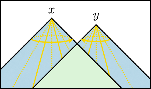
Refer to caption
Figure 25: Illustration for the envelope limit τ0𝜏0\tau\to 0 in Eq. (D.4). For each yellow line (which corresponds to the propagation line of a wall fragment), the time integration from the upper endpoint to the lower endpoint is performed in the first place. The dependence on the lower endpoint appear in Eq. (D.4) as txnisubscript𝑡𝑥𝑛𝑖t_{xni} or tynisubscript𝑡𝑦𝑛𝑖t_{yni} through the {\mathcal{E}} function.

D.2 T(x)T(y)delimited-⟨⟩𝑇𝑥delimited-⟨⟩𝑇𝑦\left<T(x)\right>\left<T(y)\right> subtraction

Numerically, the double-bubble spectrum (D.4) shows a poor convergence especially when τ𝜏\tau is much larger than 1/β1𝛽1/\beta. There is a physical reason for this behavior. Below we first explain the reason, and then provide a remedy for it.

First remember that 1/β1𝛽1/\beta determines the typical timescale from bubble nucleation to collisions (see the arguments around Eq. (2.24)). Then suppose that τ𝜏\tau is much larger than 1/β1𝛽1/\beta. The energy and momentum of the bubble walls decrease only with power-law after collisions for time τsimilar-toabsent𝜏\sim\tau, and then vanishes rapidly. What makes the poor convergence is such long-lasting walls. In order to explain how such walls cause a problem, we fix the evaluation points x𝑥x and y𝑦y so that both time and spacial separations of them are much smaller than τ𝜏\tau (but not necessarily smaller than 1/β1𝛽1/\beta). These evaluation points can be either timelike or spacelike, because both contributions exist in the double-bubble beyond the envelope. Then, as shown in Fig. 26 with the yellow circles numbered from 111 to 444, the energy-momentum tensor at these evaluation points is contributed by bubble walls from every direction which nucleated far from the evaluation points.

Let us consider the evaluation point x𝑥x for the moment, and see how these wall fragments contribute to the energy-momentum tensor at x𝑥x. If they come from every direction with exactly the same condition, the resulting ensemble average of the energy-momentum tensor at x𝑥x is isotropic and it does not contribute to the GW spectrum. We used similar arguments in Appendix A.4: we restricted the integration regions for txnsubscript𝑡𝑥𝑛t_{xn} and tynsubscript𝑡𝑦𝑛t_{yn} before tmaxsubscript𝑡maxt_{\rm max}, because those bubbles which nucleate after tmaxsubscript𝑡maxt_{\rm max} give an isotropic contribution after taking the ensemble average. However, in the present case, the wall fragments do not necessarily come from every direction in the same way. Given that the y𝑦y-bubble has nucleated somewhere, x𝑥x-fragment tend not to come from the direction where y𝑦y-bubble has nucleated. Fig. 26 illustrates this. If the y𝑦y-bubble has already nucleated at point 111, the x𝑥x-bubble cannot nucleate around that point (because spacial regions around the y𝑦y-bubble soon experience the transition from the false to true vacuum) or tends to be weaker even if it nucleates (because such a bubble soon collides with the y𝑦y-bubble). If the y𝑦y-bubble has nucleated at point 222, the x𝑥x-bubble tends not to nucleate or tends to be weaker around that point. In this sense, what breaks the isotropy is the correlation between the two bubbles.

The above arguments give us two different viewpoints on the double-bubble contribution:

  • All the nucleation patterns of the x𝑥x- and y𝑦y-bubbles such as pattern 111 to 444 in Fig. 26 sum up to give the GW spectrum.

  • Most of the nucleation patterns, like pattern 333 or 444 in Fig. 26, do not contribute to the GW spectrum because they give only isotropic contributions. Only when the two nucleation points have correlation, like pattern 111 or 222, is the isotropy broken and contributions to the GW spectrum arise.

These two viewpoints give the same GW spectrum, but require different numerics. The first one gives the spectrum only after summing up the contributions from all directions. Eq. (D.4) is based on this viewpoint, and therefore shows a poor convergence. Hence, it would be natural to look for an expression based on the second viewpoint. It is provided by subtracting T(x)T(y)delimited-⟨⟩𝑇𝑥delimited-⟨⟩𝑇𝑦\left<T(x)\right>\left<T(y)\right>. We explain this below.

The system we consider in this paper is isotropic, and therefore Eq. (2.37) with T(x)T(y)delimited-⟨⟩𝑇𝑥𝑇𝑦\left<T(x)T(y)\right> replaced by T(x)T(y)delimited-⟨⟩𝑇𝑥delimited-⟨⟩𝑇𝑦\left<T(x)\right>\left<T(y)\right> vanishes due to the projection operator. We denote the unequal-time correlator ΠΠ\Pi with such a replacement by ΠsubscriptΠ\Pi_{\infty}, where the meaning of the subscript will be made clear soon. Correspondingly, we obtain ΔsubscriptΔ\Delta_{\infty} by substituting ΠsubscriptΠ\Pi_{\infty} instead of ΠΠ\Pi into Eq. (2.43). These ΠsubscriptΠ\Pi_{\infty} and ΔsubscriptΔ\Delta_{\infty} are strictly zero, but we calculate them anyway. They can be calculated by following a similar procedure to Appendix B.4. However, there is a straightforward way to derive the resulting expression: taking rxi,yisubscript𝑟𝑥𝑖𝑦𝑖r_{xi,yi}\to\infty in Eq. (D.4). This is because considering T(x)T(y)delimited-⟨⟩𝑇𝑥delimited-⟨⟩𝑇𝑦\left<T(x)\right>\left<T(y)\right> corresponds to considering two copies of the system which are unrelated with each other, and calculate T(x)delimited-⟨⟩𝑇𝑥\left<T(x)\right> and T(y)delimited-⟨⟩𝑇𝑦\left<T(y)\right> in each of the two, respectively. Such two uncorrelated systems are effectively realized by taking rxi,yisubscript𝑟𝑥𝑖𝑦𝑖r_{xi,yi}\to\infty limit. In this limit, the spacelike theta function always gives unity and can be eliminated from the expression. Also, {\mathcal{E}} functions vanish because txnisubscript𝑡𝑥𝑛𝑖t_{xni} and tynisubscript𝑡𝑦𝑛𝑖t_{yni} go to -\infty. In addition, the {\mathcal{I}} function is replaced by subscript{\mathcal{I}}_{\infty}, where

(tx,y)subscriptsubscript𝑡𝑥𝑦\displaystyle{\mathcal{I}}_{\infty}(t_{x,y}) =8π[etx,y/2+etx,y/2].absent8𝜋delimited-[]superscript𝑒subscript𝑡𝑥𝑦2superscript𝑒subscript𝑡𝑥𝑦2\displaystyle=8\pi\left[e^{t_{x,y}/2}+e^{-t_{x,y}/2}\right]. (D.6)

As a result, we obtain the following expression for the double-bubble spectrum

Δ(d)=superscriptΔ𝑑absent\displaystyle\Delta^{(d)}= Δ(d)ΔsuperscriptΔ𝑑subscriptΔ\displaystyle\;\Delta^{(d)}-\Delta_{\infty}
=\displaystyle= 𝑑tx,y0𝑑rv0𝑑tx,xi0𝑑ty,yi11𝑑cxn11𝑑cyn02π𝑑ϕxn,ynsuperscriptsubscriptdifferential-dsubscript𝑡𝑥𝑦superscriptsubscript0differential-dsubscript𝑟𝑣superscriptsubscript0differential-dsubscript𝑡𝑥𝑥𝑖superscriptsubscript0differential-dsubscript𝑡𝑦𝑦𝑖superscriptsubscript11differential-dsubscript𝑐𝑥𝑛superscriptsubscript11differential-dsubscript𝑐𝑦𝑛superscriptsubscript02𝜋differential-dsubscriptitalic-ϕ𝑥𝑛𝑦𝑛\displaystyle\int_{-\infty}^{\infty}dt_{x,y}\int_{0}^{\infty}dr_{v}\int_{0}^{\infty}dt_{x,xi}\int_{0}^{\infty}dt_{y,yi}\int_{-1}^{1}dc_{xn}\int_{-1}^{1}dc_{yn}\int_{0}^{2\pi}d\phi_{xn,yn}
12v3k312superscript𝑣3superscript𝑘3\displaystyle 12v^{3}k^{3} [(1+1τ)2e(tx,xi+ty,yi)/τ×[Θsp(xi,yi)[1(τ;txi,xni)][1(τ;tyi,yni)](txi,yi,rxi,yi/v)21(txi,yi)2]×rv2[j0(vkrv)𝒦0(nxn,nyn)+j1(vkrv)vkrv𝒦1(nxn,nyn)+j2(vkrv)(vkrv)2𝒦2(nxn,nyn)]×cos(ktx,y)].delimited-[]matrixsuperscript11𝜏2superscript𝑒subscript𝑡𝑥𝑥𝑖subscript𝑡𝑦𝑦𝑖𝜏absentdelimited-[]subscriptΘspsubscript𝑥𝑖subscript𝑦𝑖delimited-[]1𝜏subscript𝑡𝑥𝑖𝑥𝑛𝑖delimited-[]1𝜏subscript𝑡𝑦𝑖𝑦𝑛𝑖superscriptsubscript𝑡𝑥𝑖𝑦𝑖subscript𝑟𝑥𝑖𝑦𝑖𝑣21subscriptsuperscriptsubscript𝑡𝑥𝑖𝑦𝑖2absentsuperscriptsubscript𝑟𝑣2delimited-[]subscript𝑗0𝑣𝑘subscript𝑟𝑣subscript𝒦0subscript𝑛𝑥𝑛subscript𝑛𝑦𝑛subscript𝑗1𝑣𝑘subscript𝑟𝑣𝑣𝑘subscript𝑟𝑣subscript𝒦1subscript𝑛𝑥𝑛subscript𝑛𝑦𝑛subscript𝑗2𝑣𝑘subscript𝑟𝑣superscript𝑣𝑘subscript𝑟𝑣2subscript𝒦2subscript𝑛𝑥𝑛subscript𝑛𝑦𝑛absent𝑘subscript𝑡𝑥𝑦\displaystyle\left[\begin{matrix}[l]\displaystyle\;\left(1+\frac{1}{\tau}\right)^{2}e^{-(t_{x,xi}+t_{y,yi})/\tau}\\[6.45831pt] \displaystyle\times\left[\Theta_{\rm sp}(x_{i},y_{i})\frac{\left[1-{\mathcal{E}}(\tau;t_{xi,xni})\right]\left[1-{\mathcal{E}}(\tau;t_{yi,yni})\right]}{{\mathcal{I}}(t_{xi,yi},r_{xi,yi}/v)^{2}}-\frac{1}{{\mathcal{I}}_{\infty}(t_{xi,yi})^{2}}\right]\\[8.61108pt] \displaystyle\times\;r_{v}^{2}\left[j_{0}(vkr_{v}){\mathcal{K}}_{0}(n_{xn},n_{yn})+\frac{j_{1}(vkr_{v})}{vkr_{v}}{\mathcal{K}}_{1}(n_{xn},n_{yn})+\frac{j_{2}(vkr_{v})}{(vkr_{v})^{2}}{\mathcal{K}}_{2}(n_{xn},n_{yn})\right]\\[8.61108pt] \times\cos(kt_{x,y})\end{matrix}\right]. (D.7)

This expression properly realizes the second viewpoint explained above: for bubble nucleation patterns like 333 or 444 in Fig. 26, the second line in the square parenthesis almost vanishes (note that for a large separation 1/βmuch-greater-thanabsent1𝛽\gg 1/\beta between the nucleation points like pattern 333 or 444, the separation between the interception points tend to be also large). Also, one can check that ΔsubscriptΔ\Delta_{\infty} vanishes: the dependence on the propagation directions appears only in the 𝒦𝒦{\mathcal{K}} functions, which vanish after cxnsubscript𝑐𝑥𝑛c_{xn}, cynsubscript𝑐𝑦𝑛c_{yn} and ϕxn,ynsubscriptitalic-ϕ𝑥𝑛𝑦𝑛\phi_{xn,yn} integrations. We use Eq. (D.7) in the numerical evaluation in Sec. 4.
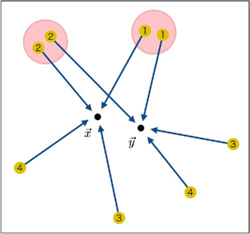
Refer to caption
Figure 26: Illustration for how correlation between the x𝑥x- and y𝑦y-bubbles arises. If the y𝑦y-bubble nucleates at point 111, the x𝑥x-bubble tend not to nucleate around the y𝑦y-bubble nucleation point, or tend to have a weak bubble wall even if it nucleates around there, due to the existence of the y𝑦y-bubble. Such a realization pattern is denoted by label 111. The pink circles denote the correlation region, which typically have size 1/βsimilar-toabsent1𝛽\sim 1/\beta. The same applies to the nucleation pattern 222. For the nucleation patterns 333 or 444, the x𝑥x- and y𝑦y-bubbles nucleate and experience subsequent collisions with other bubbles almost independently of each other. For long-lasting walls (i.e. τ1/βmuch-greater-than𝜏1𝛽\tau\gg 1/\beta), there are much more cases like 333 or 444 than like 111 or 222.

In the following, we derive the expression for ΔsubscriptΔ\Delta_{\infty} one by one for completeness. The procedure is almost the same as Sec. B.4. First note that there are two types of contributions to T(x)delimited-⟨⟩𝑇𝑥\left<T(x)\right>:

  • U𝑈U : x𝑥x-fragment remains uncollided at the evaluation point.

  • C𝐶C : x𝑥x-fragment has already been intercepted at the evaluation point.

They are written as

T(x)(U)superscriptdelimited-⟨⟩𝑇𝑥𝑈\displaystyle\left<T(x)\right>^{(U)} =txdtxndΩxneI(x)(x;xi=x;xn),\displaystyle=\int_{-\infty}^{t_{x}}dt_{xn}\int d\Omega_{xn}\;e^{-I(x)}{\mathcal{F}}_{\infty}(x;x_{i}=x;x_{n}), (D.8)
T(x)(C)superscriptdelimited-⟨⟩𝑇𝑥𝐶\displaystyle\left<T(x)\right>^{(C)} =tx𝑑txntxntx𝑑txi𝑑Ωxn[I(xi)eI(xi)]txi(x;xi;xn),absentsuperscriptsubscriptsubscript𝑡𝑥differential-dsubscript𝑡𝑥𝑛superscriptsubscriptsubscript𝑡𝑥𝑛subscript𝑡𝑥differential-dsubscript𝑡𝑥𝑖differential-dsubscriptΩ𝑥𝑛subscriptdelimited-[]𝐼subscript𝑥𝑖superscript𝑒𝐼subscript𝑥𝑖𝑡𝑥𝑖subscript𝑥subscript𝑥𝑖subscript𝑥𝑛\displaystyle=\int_{-\infty}^{t_{x}}dt_{xn}\int_{t_{xn}}^{t_{x}}dt_{xi}\int d\Omega_{xn}\left[I(x_{i})e^{-I(x_{i})}\right]_{txi}{\mathcal{F}}_{\infty}(x;x_{i};x_{n}), (D.9)

where subscript{\mathcal{F}}_{\infty} is given by

(x,xi,xn)subscript𝑥subscript𝑥𝑖subscript𝑥𝑛\displaystyle{\mathcal{F}}_{\infty}(x,x_{i},x_{n}) =rxn(d)2lBΓ(txn)(4π3rxn(d)3κρ014πrxn(d)2lB)rB(txi,txn)3rxn(d)3D(tx,txi,txn).absentsuperscriptsubscript𝑟𝑥𝑛𝑑2subscript𝑙𝐵Γsubscript𝑡𝑥𝑛4𝜋3superscriptsubscript𝑟𝑥𝑛𝑑3𝜅subscript𝜌014𝜋superscriptsubscript𝑟𝑥𝑛𝑑2subscript𝑙𝐵subscript𝑟𝐵superscriptsubscript𝑡𝑥𝑖subscript𝑡𝑥𝑛3superscriptsubscript𝑟𝑥𝑛𝑑3𝐷subscript𝑡𝑥subscript𝑡𝑥𝑖subscript𝑡𝑥𝑛\displaystyle=r_{xn}^{(d)2}l_{B}\Gamma(t_{xn})\;\left(\frac{4\pi}{3}r_{xn}^{(d)3}\kappa\rho_{0}\frac{1}{4\pi r_{xn}^{(d)2}l_{B}}\right)\frac{r_{B}(t_{xi},t_{xn})^{3}}{r_{xn}^{(d)3}}D(t_{x},t_{xi},t_{xn}). (D.10)

Note that now the false vacuum probability has only one argument. These two are combined to give

T(x)(U+C)superscriptdelimited-⟨⟩𝑇𝑥𝑈𝐶\displaystyle\left<T(x)\right>^{(U+C)} =tx𝑑txntxntx𝑑txi𝑑ΩxneI(xi)[(x;xi;xn)]txi,absentsuperscriptsubscriptsubscript𝑡𝑥differential-dsubscript𝑡𝑥𝑛superscriptsubscriptsubscript𝑡𝑥𝑛subscript𝑡𝑥differential-dsubscript𝑡𝑥𝑖differential-dsubscriptΩ𝑥𝑛superscript𝑒𝐼subscript𝑥𝑖subscriptdelimited-[]subscript𝑥subscript𝑥𝑖subscript𝑥𝑛𝑡𝑥𝑖\displaystyle=\int_{-\infty}^{t_{x}}dt_{xn}\int_{t_{xn}}^{t_{x}}dt_{xi}\int d\Omega_{xn}\;e^{-I(x_{i})}\left[{\mathcal{F}}_{\infty}(x;x_{i};x_{n})\right]_{txi}, (D.11)

where we used (x;xi=xn;xn)=0{\mathcal{F}}_{\infty}(x;x_{i}=x_{n};x_{n})=0. A similar expression is obtained for T(y)(U+C)superscriptdelimited-⟨⟩𝑇𝑦𝑈𝐶\left<T(y)\right>^{(U+C)}, and we obtain the following expression for ΔsubscriptΔ\Delta_{\infty} for a general nucleation rate and the damping function

Δ=subscriptΔabsent\displaystyle\Delta_{\infty}= 𝑑tx𝑑tysuperscriptsubscriptdifferential-dsubscript𝑡𝑥superscriptsubscriptdifferential-dsubscript𝑡𝑦\displaystyle\int_{-\infty}^{\infty}dt_{x}\int_{-\infty}^{\infty}dt_{y}
0𝑑rtx𝑑txnty𝑑tyntxntx𝑑txitynty𝑑tyi11𝑑cxn11𝑑cyn02π𝑑ϕxn,ynsuperscriptsubscript0differential-d𝑟superscriptsubscriptsubscript𝑡𝑥differential-dsubscript𝑡𝑥𝑛superscriptsubscriptsubscript𝑡𝑦differential-dsubscript𝑡𝑦𝑛superscriptsubscriptsubscript𝑡𝑥𝑛subscript𝑡𝑥differential-dsubscript𝑡𝑥𝑖superscriptsubscriptsubscript𝑡𝑦𝑛subscript𝑡𝑦differential-dsubscript𝑡𝑦𝑖superscriptsubscript11differential-dsubscript𝑐𝑥𝑛superscriptsubscript11differential-dsubscript𝑐𝑦𝑛superscriptsubscript02𝜋differential-dsubscriptitalic-ϕ𝑥𝑛𝑦𝑛\displaystyle\int_{0}^{\infty}dr\int_{-\infty}^{t_{x}}dt_{xn}\int_{-\infty}^{t_{y}}dt_{yn}\int_{t_{xn}}^{t_{x}}dt_{xi}\int_{t_{yn}}^{t_{y}}dt_{yi}\int_{-1}^{1}dc_{xn}\int_{-1}^{1}dc_{yn}\int_{0}^{2\pi}d\phi_{xn,yn}
k33superscript𝑘33\displaystyle\frac{k^{3}}{3} [eI(xi)eI(yi)Γ(txn)Γ(tyn)×r2[j0(kr)𝒦0(nxn,nyn)+j1(kr)kr𝒦1(nxn,nyn)+j2(kr)(kr)2𝒦2(nxn,nyn)]×txi[rB(txi,txn)3D(tx,txi,tyn)]tyi[rB(tyi,tyn)3D(ty,tyi,tyn)]cos(ktx,y)],\displaystyle\left[\begin{matrix}[l]\displaystyle\;e^{-I(x_{i})}e^{-I(y_{i})}\Gamma(t_{xn})\Gamma(t_{yn})\\[4.30554pt] \displaystyle\times\;r^{2}\left[j_{0}(kr){\mathcal{K}}_{0}(n_{xn},n_{yn})+\frac{j_{1}(kr)}{kr}{\mathcal{K}}_{1}(n_{xn},n_{yn})+\frac{j_{2}(kr)}{(kr)^{2}}{\mathcal{K}}_{2}(n_{xn},n_{yn})\right]\\[8.61108pt] \displaystyle\times\;\partial_{txi}\left[r_{B}(t_{xi},t_{xn})^{3}D(t_{x},t_{xi},t_{yn})\right]\partial_{tyi}\left[r_{B}(t_{yi},t_{yn})^{3}D(t_{y},t_{yi},t_{yn})\right]\cos(kt_{x,y})\end{matrix}\right], (D.12)

Following the same procedure as Appendix D.1, we obtain the following expression for the nucleation rate (2.24) and the damping function (2.23):

Δ=subscriptΔabsent\displaystyle\Delta_{\infty}= 𝑑tx,y0𝑑rv0𝑑tx,xi0𝑑ty,yi11𝑑cxn11𝑑cyn02π𝑑ϕxn,ynsuperscriptsubscriptdifferential-dsubscript𝑡𝑥𝑦superscriptsubscript0differential-dsubscript𝑟𝑣superscriptsubscript0differential-dsubscript𝑡𝑥𝑥𝑖superscriptsubscript0differential-dsubscript𝑡𝑦𝑦𝑖superscriptsubscript11differential-dsubscript𝑐𝑥𝑛superscriptsubscript11differential-dsubscript𝑐𝑦𝑛superscriptsubscript02𝜋differential-dsubscriptitalic-ϕ𝑥𝑛𝑦𝑛\displaystyle\int_{-\infty}^{\infty}dt_{x,y}\int_{0}^{\infty}dr_{v}\int_{0}^{\infty}dt_{x,xi}\int_{0}^{\infty}dt_{y,yi}\int_{-1}^{1}dc_{xn}\int_{-1}^{1}dc_{yn}\int_{0}^{2\pi}d\phi_{xn,yn}
12v3k312superscript𝑣3superscript𝑘3\displaystyle 12v^{3}k^{3} [(1+1τ)2e(tx,xi+ty,yi)/τ(txi,yi)2×rv2[j0(vkrv)𝒦0(nxn,nyn)+j1(vkrv)vkrv𝒦1(nxn,nyn)+j2(vkrv)(vkrv)2𝒦2(nxn,nyn)]×cos(ktx,y)].delimited-[]matrixsuperscript11𝜏2superscript𝑒subscript𝑡𝑥𝑥𝑖subscript𝑡𝑦𝑦𝑖𝜏subscriptsuperscriptsubscript𝑡𝑥𝑖𝑦𝑖2absentsuperscriptsubscript𝑟𝑣2delimited-[]subscript𝑗0𝑣𝑘subscript𝑟𝑣subscript𝒦0subscript𝑛𝑥𝑛subscript𝑛𝑦𝑛subscript𝑗1𝑣𝑘subscript𝑟𝑣𝑣𝑘subscript𝑟𝑣subscript𝒦1subscript𝑛𝑥𝑛subscript𝑛𝑦𝑛subscript𝑗2𝑣𝑘subscript𝑟𝑣superscript𝑣𝑘subscript𝑟𝑣2subscript𝒦2subscript𝑛𝑥𝑛subscript𝑛𝑦𝑛absent𝑘subscript𝑡𝑥𝑦\displaystyle\left[\begin{matrix}[l]\displaystyle\;\left(1+\frac{1}{\tau}\right)^{2}\frac{e^{-(t_{x,xi}+t_{y,yi})/\tau}}{{\mathcal{I}}_{\infty}(t_{xi,yi})^{2}}\\[8.61108pt] \displaystyle\times\;r_{v}^{2}\left[j_{0}(vkr_{v}){\mathcal{K}}_{0}(n_{xn},n_{yn})+\frac{j_{1}(vkr_{v})}{vkr_{v}}{\mathcal{K}}_{1}(n_{xn},n_{yn})+\frac{j_{2}(vkr_{v})}{(vkr_{v})^{2}}{\mathcal{K}}_{2}(n_{xn},n_{yn})\right]\\[8.61108pt] \times\cos(kt_{x,y})\end{matrix}\right]. (D.13)

Appendix E Analytic proof on the spectrum behavior

In this appendix we give proofs on the behavior of the GW spectrum for small k𝑘k region in τ𝜏\tau\to\infty limit. In Sec. 4 and Appendix G we have numerically seen that the spectrum behaves linear in k𝑘k in τ𝜏\tau\to\infty limit. The aim of this appendix is to justify this behavior by analytic arguments. In the following, note that we adopt β=1𝛽1\beta=1 unit.

E.1 Single-bubble spectrum

Let us start with Eq. (B.10) with D=1𝐷1D=1 (long-lasting limit τ𝜏\tau\to\infty) and rxi,yisubscript𝑟𝑥𝑖𝑦𝑖r_{xi,yi} given by Eq. (B.14). The key to observe the behavior of the spectrum for small k𝑘k is to classify the integration variables depending on the values they typically take:

  • Variable r𝑟r takes 1/ksimilar-toabsent1𝑘\sim 1/k, because GWs with wavenumber k𝑘k are mostly sourced by objects with distance 1/ksimilar-toabsent1𝑘\sim 1/k away from each other.

  • Variables tx,nsubscript𝑡𝑥𝑛t_{x,n} and ty,nsubscript𝑡𝑦𝑛t_{y,n} take 1/vksimilar-toabsent1𝑣𝑘\sim 1/vk, because x𝑥x- and y𝑦y-fragments propagate distances r1/ksimilar-toabsent𝑟similar-to1𝑘\sim r\sim 1/k after nucleation to the evaluation times.

  • Variables txi,nsubscript𝑡𝑥𝑖𝑛t_{xi,n} and tyi,nsubscript𝑡𝑦𝑖𝑛t_{yi,n} take 1similar-toabsent1\sim 1, because the whole space is covered by bubbles typically with timescale 1similar-toabsent1\sim 1.

Based on these observations, we first rewrite the integration variable in Eq. (B.10) as

𝑑tx𝑑tyv|tx,y|𝑑rtmax𝑑tntntx𝑑txitnty𝑑tyisuperscriptsubscriptdifferential-dsubscript𝑡𝑥superscriptsubscriptdifferential-dsubscript𝑡𝑦superscriptsubscript𝑣subscript𝑡𝑥𝑦differential-d𝑟superscriptsubscriptsubscript𝑡maxdifferential-dsubscript𝑡𝑛superscriptsubscriptsubscript𝑡𝑛subscript𝑡𝑥differential-dsubscript𝑡𝑥𝑖superscriptsubscriptsubscript𝑡𝑛subscript𝑡𝑦differential-dsubscript𝑡𝑦𝑖\displaystyle\int_{-\infty}^{\infty}dt_{x}\int_{-\infty}^{\infty}dt_{y}\int_{v|t_{x,y}|}^{\infty}dr\int_{-\infty}^{t_{\rm max}}dt_{n}\int_{t_{n}}^{t_{x}}dt_{xi}\int_{t_{n}}^{t_{y}}dt_{yi}
=0𝑑tx,n0𝑑ty,nv|tx,nty,n|v(tx,n+ty,n)𝑑r𝑑tn0tx,n𝑑txi,n0ty,n𝑑tyi,n.superscriptsubscript0differential-dsubscript𝑡𝑥𝑛superscriptsubscript0differential-dsubscript𝑡𝑦𝑛superscriptsubscript𝑣subscript𝑡𝑥𝑛subscript𝑡𝑦𝑛𝑣subscript𝑡𝑥𝑛subscript𝑡𝑦𝑛differential-d𝑟superscriptsubscriptdifferential-dsubscript𝑡𝑛superscriptsubscript0subscript𝑡𝑥𝑛differential-dsubscript𝑡𝑥𝑖𝑛superscriptsubscript0subscript𝑡𝑦𝑛differential-dsubscript𝑡𝑦𝑖𝑛\displaystyle\;\;\;\;=\;\;\;\;\int_{0}^{\infty}dt_{x,n}\int_{0}^{\infty}dt_{y,n}\int_{v|t_{x,n}-t_{y,n}|}^{v(t_{x,n}+t_{y,n})}dr\int_{-\infty}^{\infty}dt_{n}\int_{0}^{t_{x,n}}dt_{xi,n}\int_{0}^{t_{y,n}}dt_{yi,n}. (E.1)

Note that time variables txnsubscript𝑡𝑥𝑛t_{xn}, tynsubscript𝑡𝑦𝑛t_{yn}, txisubscript𝑡𝑥𝑖t_{xi} and tyisubscript𝑡𝑦𝑖t_{yi} are now expressed in terms of differences from tnsubscript𝑡𝑛t_{n}. Then we rescale those variables which typically take 1/ksimilar-toabsent1𝑘\sim 1/k or 1/vksimilar-toabsent1𝑣𝑘\sim 1/vk by multiplying k𝑘k:

Δ(s)=superscriptΔ𝑠absent\displaystyle\Delta^{(s)}= 0𝑑tx,n0𝑑ty,nv|tx,nty,n|v(tx,n+ty,n)𝑑r𝑑tn0tx,n/k𝑑txi,n0ty,n/k𝑑tyi,nsuperscriptsubscript0differential-dsubscriptsuperscript𝑡𝑥𝑛superscriptsubscript0differential-dsubscriptsuperscript𝑡𝑦𝑛superscriptsubscript𝑣subscriptsuperscript𝑡𝑥𝑛subscriptsuperscript𝑡𝑦𝑛𝑣subscriptsuperscript𝑡𝑥𝑛subscriptsuperscript𝑡𝑦𝑛differential-dsuperscript𝑟superscriptsubscriptdifferential-dsubscript𝑡𝑛superscriptsubscript0subscriptsuperscript𝑡𝑥𝑛𝑘differential-dsubscript𝑡𝑥𝑖𝑛superscriptsubscript0subscriptsuperscript𝑡𝑦𝑛𝑘differential-dsubscript𝑡𝑦𝑖𝑛\displaystyle\int_{0}^{\infty}dt^{\prime}_{x,n}\int_{0}^{\infty}dt^{\prime}_{y,n}\int_{v|t^{\prime}_{x,n}-t^{\prime}_{y,n}|}^{v(t^{\prime}_{x,n}+t^{\prime}_{y,n})}dr^{\prime}\int_{-\infty}^{\infty}dt_{n}\int_{0}^{t^{\prime}_{x,n}/k}dt_{xi,n}\int_{0}^{t^{\prime}_{y,n}/k}dt_{yi,n}
k3𝑘3\displaystyle\frac{k}{3} [eI(xi,yi)Γ(tn)rrxn(s)ryn(s)×[j0(r)𝒦0(nxn×,nyn×)+j1(r)r𝒦1(nxn×,nyn×)+j2(r)r2𝒦2(nxn×,nyn×)]×txi[rB(txi,tn)3]tyi[rB(tyi,tn)3]cos(k(tx,nty,n))],\displaystyle\left[\begin{matrix}[l]\displaystyle\;e^{-I(x_{i},y_{i})}\;\Gamma(t_{n})\;\frac{r^{\prime}}{r_{xn}^{{}^{\prime}(s)}r_{yn}^{{}^{\prime}(s)}}\\ \displaystyle\times\left[j_{0}(r^{\prime}){\mathcal{K}}_{0}(n_{xn\times},n_{yn\times})+\frac{j_{1}(r^{\prime})}{r^{\prime}}{\mathcal{K}}_{1}(n_{xn\times},n_{yn\times})+\frac{j_{2}(r^{\prime})}{r^{{}^{\prime}2}}{\mathcal{K}}_{2}(n_{xn\times},n_{yn\times})\right]\\[10.76385pt] \displaystyle\times\;\partial_{txi}\left[r_{B}(t_{xi},t_{n})^{3}\right]\partial_{tyi}\left[r_{B}(t_{yi},t_{n})^{3}\right]\cos(k(t^{\prime}_{x,n}-t^{\prime}_{y,n}))\end{matrix}\right], (E.2)

where variables with primes mean k\bullet^{\prime}\equiv k\bullet. Now we argue that this expression does not depend on k𝑘k except for the overall k𝑘k in the small k𝑘k limit:

  • The upper limits for txi,nsubscript𝑡𝑥𝑖𝑛t_{xi,n} and tyi,nsubscript𝑡𝑦𝑖𝑛t_{yi,n} go to infinity and thus become independent of k𝑘k.

  • The variables rxn(s)=vtx,nr^{{}^{\prime}(s)}_{xn}=vt^{\prime}_{x,n} and ryn(s)=vty,nr^{{}^{\prime}(s)}_{yn}=vt^{\prime}_{y,n} do not depend on k𝑘k.

  • I(xi,yi)=v3Γetn+(txi,n+tyi,n)/2(txi,ntyi,n,rxi,yi)𝐼subscript𝑥𝑖subscript𝑦𝑖superscript𝑣3subscriptΓsuperscript𝑒subscript𝑡𝑛subscript𝑡𝑥𝑖𝑛subscript𝑡𝑦𝑖𝑛2subscript𝑡𝑥𝑖𝑛subscript𝑡𝑦𝑖𝑛subscript𝑟𝑥𝑖𝑦𝑖I(x_{i},y_{i})=v^{3}\Gamma_{*}e^{t_{n}+(t_{xi,n}+t_{yi,n})/2}{\mathcal{I}}(t_{xi,n}-t_{yi,n},r_{xi,yi}) does not depend on k𝑘k. Note that rxi,yisubscript𝑟𝑥𝑖𝑦𝑖r_{xi,yi} is independent of k𝑘k. This is because, in Eq. (B.14), cxyn×subscript𝑐𝑥𝑦𝑛c_{xyn\times} is written in terms of cxn×subscript𝑐𝑥𝑛c_{xn\times}, cyn×subscript𝑐𝑦𝑛c_{yn\times}, sxn×subscript𝑠𝑥𝑛s_{xn\times} and syn×subscript𝑠𝑦𝑛s_{yn\times}, which can be expressed without k𝑘k dependence:

    cxn×subscript𝑐𝑥𝑛\displaystyle c_{xn\times} =r2+rxn(s)2ryn(s)22rrxn(s),cyn×=r2+ryn(s)2rxn(s)22rryn(s).\displaystyle=-\frac{r^{{}^{\prime}2}+r_{xn}^{{}^{\prime}(s)2}-r_{yn}^{{}^{\prime}(s)2}}{2r^{\prime}r_{xn}^{{}^{\prime}(s)}},\;\;\;\;c_{yn\times}=\frac{r^{{}^{\prime}2}+r_{yn}^{{}^{\prime}(s)2}-r_{xn}^{{}^{\prime}(s)2}}{2r^{\prime}r_{yn}^{{}^{\prime}(s)}}. (E.3)
  • The angular variables nxn×subscript𝑛𝑥𝑛n_{xn\times} and nyn×subscript𝑛𝑦𝑛n_{yn\times} do not depend on k𝑘k because of the same reason as above.

Therefore Δ(s)superscriptΔ𝑠\Delta^{(s)} behaves linearly in k𝑘k for small k𝑘k in the long-lasting limit of the bubble walls.

E.2 Double-bubble spectrum

In the double-bubble case the procedure is basically the same as the single-bubble case. However, in contrast to the single-bubble case, it might be nontrivial that rxi,yisubscript𝑟𝑥𝑖𝑦𝑖r_{xi,yi} takes 1similar-toabsent1\sim 1, not 1/ksimilar-toabsent1𝑘\sim 1/k, at first sight (see Eq. (B.21)). First let us check by a rough argument that rxi,yisubscript𝑟𝑥𝑖𝑦𝑖r_{xi,yi} typically does not take 1/ksimilar-toabsent1𝑘\sim 1/k. We consider Eq. (B.19) with the subtraction of Eq. (D.12). It contains a factor

Θsp(xi,yn)Θsp(xn,yi)eI(xi,yi)eI(xi)eI(yi).subscriptΘspsubscript𝑥𝑖subscript𝑦𝑛subscriptΘspsubscript𝑥𝑛subscript𝑦𝑖superscript𝑒𝐼subscript𝑥𝑖subscript𝑦𝑖superscript𝑒𝐼subscript𝑥𝑖superscript𝑒𝐼subscript𝑦𝑖\displaystyle\Theta_{\rm sp}(x_{i},y_{n})\Theta_{\rm sp}(x_{n},y_{i})e^{-I(x_{i},y_{i})}-e^{-I(x_{i})}e^{-I(y_{i})}. (E.4)

Suppose that rxi,yi1/ksimilar-tosubscript𝑟𝑥𝑖𝑦𝑖1𝑘r_{xi,yi}\sim 1/k. We can safely assume that txisubscript𝑡𝑥𝑖t_{xi} and tyisubscript𝑡𝑦𝑖t_{yi} are different by only 1similar-toabsent1\sim 1 or smaller, because otherwise at least either of the nucleation times txnsubscript𝑡𝑥𝑛t_{xn} and tynsubscript𝑡𝑦𝑛t_{yn} (which are typically only 1similar-toabsent1\sim 1 away from txisubscript𝑡𝑥𝑖t_{xi} and tyisubscript𝑡𝑦𝑖t_{yi}) is away from the typical nucleation times by more than 1similar-toabsent1\sim 1, and the probability for such a bubble configuration to occur is exponentially suppressed. Then we can set Θsp(xi,yn)Θsp(xn,yi)subscriptΘspsubscript𝑥𝑖subscript𝑦𝑛subscriptΘspsubscript𝑥𝑛subscript𝑦𝑖\Theta_{\rm sp}(x_{i},y_{n})\Theta_{\rm sp}(x_{n},y_{i}) to unity. Now we see that eI(xi,yi)superscript𝑒𝐼subscript𝑥𝑖subscript𝑦𝑖e^{-I(x_{i},y_{i})} and eI(xi)eI(yi)superscript𝑒𝐼subscript𝑥𝑖superscript𝑒𝐼subscript𝑦𝑖e^{-I(x_{i})}e^{-I(y_{i})} almost cancels out (eI(xi,yi)eI(xi)eI(yi)e𝒪(1)/k×eI(xi,yi)similar-tosuperscript𝑒𝐼subscript𝑥𝑖subscript𝑦𝑖superscript𝑒𝐼subscript𝑥𝑖superscript𝑒𝐼subscript𝑦𝑖superscript𝑒𝒪1𝑘superscript𝑒𝐼subscript𝑥𝑖subscript𝑦𝑖e^{-I(x_{i},y_{i})}-e^{-I(x_{i})}e^{-I(y_{i})}\sim e^{-{\mathcal{O}}(1)/k}\times e^{-I(x_{i},y_{i})}) for such a large separation rxi,yisubscript𝑟𝑥𝑖𝑦𝑖r_{xi,yi} between the interception points, and therefore such configurations give only suppressed contributions to the GW spectrum. Hence we can take rxi,yivsimilar-tosubscript𝑟𝑥𝑖𝑦𝑖𝑣r_{xi,yi}\sim v, not 1/ksimilar-toabsent1𝑘\sim 1/k, in Δ(d)ΔsuperscriptΔ𝑑subscriptΔ\Delta^{(d)}-\Delta_{\infty}, and by the same procedure as the single-bubble case, we obtain kproportional-toabsent𝑘\propto k behavior. Below we see these arguments more rigorously.

We start with Eq. (B.19) subtracted by Eq. (D.12):

Δ(d)=superscriptΔ𝑑absent\displaystyle\Delta^{(d)}= Δ(d)ΔsuperscriptΔ𝑑subscriptΔ\displaystyle\;\Delta^{(d)}-\Delta_{\infty}
=\displaystyle= 𝑑tx𝑑tysuperscriptsubscriptdifferential-dsubscript𝑡𝑥superscriptsubscriptdifferential-dsubscript𝑡𝑦\displaystyle\int_{-\infty}^{\infty}dt_{x}\int_{-\infty}^{\infty}dt_{y}
0𝑑rtx𝑑txnty𝑑tyntxntx𝑑txitynty𝑑tyi11𝑑cxn11𝑑cyn02π𝑑ϕxn,ynsuperscriptsubscript0differential-d𝑟superscriptsubscriptsubscript𝑡𝑥differential-dsubscript𝑡𝑥𝑛superscriptsubscriptsubscript𝑡𝑦differential-dsubscript𝑡𝑦𝑛superscriptsubscriptsubscript𝑡𝑥𝑛subscript𝑡𝑥differential-dsubscript𝑡𝑥𝑖superscriptsubscriptsubscript𝑡𝑦𝑛subscript𝑡𝑦differential-dsubscript𝑡𝑦𝑖superscriptsubscript11differential-dsubscript𝑐𝑥𝑛superscriptsubscript11differential-dsubscript𝑐𝑦𝑛superscriptsubscript02𝜋differential-dsubscriptitalic-ϕ𝑥𝑛𝑦𝑛\displaystyle\int_{0}^{\infty}dr\int_{-\infty}^{t_{x}}dt_{xn}\int_{-\infty}^{t_{y}}dt_{yn}\int_{t_{xn}}^{t_{x}}dt_{xi}\int_{t_{yn}}^{t_{y}}dt_{yi}\int_{-1}^{1}dc_{xn}\int_{-1}^{1}dc_{yn}\int_{0}^{2\pi}d\phi_{xn,yn}
k33superscript𝑘33\displaystyle\frac{k^{3}}{3} [[Θsp(xi,yn)Θsp(xn,yi)eI(xi,yi)eI(xi)eI(yi)]Γ(txn)Γ(tyn)×r2[j0(kr)𝒦0(nxn,nyn)+j1(kr)kr𝒦1(nxn,nyn)+j2(kr)(kr)2𝒦2(nxn,nyn)]×txi[rB(txi,txn)3]tyi[rB(tyi,tyn)3]cos(ktx,y)],\displaystyle\left[\begin{matrix}[l]\displaystyle\;\left[\Theta_{\rm sp}(x_{i},y_{n})\Theta_{\rm sp}(x_{n},y_{i})e^{-I(x_{i},y_{i})}-e^{-I(x_{i})}e^{-I(y_{i})}\right]\Gamma(t_{xn})\Gamma(t_{yn})\\[4.30554pt] \displaystyle\times\;r^{2}\left[j_{0}(kr){\mathcal{K}}_{0}(n_{xn},n_{yn})+\frac{j_{1}(kr)}{kr}{\mathcal{K}}_{1}(n_{xn},n_{yn})+\frac{j_{2}(kr)}{(kr)^{2}}{\mathcal{K}}_{2}(n_{xn},n_{yn})\right]\\[8.61108pt] \displaystyle\times\;\partial_{txi}\left[r_{B}(t_{xi},t_{xn})^{3}\right]\partial_{tyi}\left[r_{B}(t_{yi},t_{yn})^{3}\right]\cos(kt_{x,y})\end{matrix}\right], (E.5)

where we have taken D=1𝐷1D=1 (long-lasting limit τ𝜏\tau\to\infty). We rewrite the integration variable r𝑟r in terms of rirxi,yisubscript𝑟𝑖subscript𝑟𝑥𝑖𝑦𝑖r_{i}\equiv r_{xi,yi} through the relation (B.21). However, before that procedure, we replace the integration range for r𝑟r to (,)(-\infty,\infty) and compensate it by multiplying an overall factor 1/2121/2:

Δ(d)=superscriptΔ𝑑absent\displaystyle\Delta^{(d)}= 𝑑tx𝑑tysuperscriptsubscriptdifferential-dsubscript𝑡𝑥superscriptsubscriptdifferential-dsubscript𝑡𝑦\displaystyle\int_{-\infty}^{\infty}dt_{x}\int_{-\infty}^{\infty}dt_{y}
𝑑rtx𝑑txnty𝑑tyntxntx𝑑txitynty𝑑tyi11𝑑cxn11𝑑cyn02π𝑑ϕxn,ynsuperscriptsubscriptdifferential-d𝑟superscriptsubscriptsubscript𝑡𝑥differential-dsubscript𝑡𝑥𝑛superscriptsubscriptsubscript𝑡𝑦differential-dsubscript𝑡𝑦𝑛superscriptsubscriptsubscript𝑡𝑥𝑛subscript𝑡𝑥differential-dsubscript𝑡𝑥𝑖superscriptsubscriptsubscript𝑡𝑦𝑛subscript𝑡𝑦differential-dsubscript𝑡𝑦𝑖superscriptsubscript11differential-dsubscript𝑐𝑥𝑛superscriptsubscript11differential-dsubscript𝑐𝑦𝑛superscriptsubscript02𝜋differential-dsubscriptitalic-ϕ𝑥𝑛𝑦𝑛\displaystyle\int_{-\infty}^{\infty}dr\int_{-\infty}^{t_{x}}dt_{xn}\int_{-\infty}^{t_{y}}dt_{yn}\int_{t_{xn}}^{t_{x}}dt_{xi}\int_{t_{yn}}^{t_{y}}dt_{yi}\int_{-1}^{1}dc_{xn}\int_{-1}^{1}dc_{yn}\int_{0}^{2\pi}d\phi_{xn,yn}
k36superscript𝑘36\displaystyle\frac{k^{3}}{6} [[Θsp(xi,yn)Θsp(xn,yi)eI(xi,yi)eI(xi)eI(yi)]Γ(txn)Γ(tyn)×|r|2[j0(k|r|)𝒦0(nxn,nyn)+j1(k|r|)k|r|𝒦1(nxn,nyn)+j2(k|r|)(k|r|)2𝒦2(nxn,nyn)]×txi[rB(txi,txn)3]tyi[rB(tyi,tyn)3]cos(ktx,y)],\displaystyle\left[\begin{matrix}[l]\displaystyle\;\left[\Theta_{\rm sp}(x_{i},y_{n})\Theta_{\rm sp}(x_{n},y_{i})e^{-I(x_{i},y_{i})}-e^{-I(x_{i})}e^{-I(y_{i})}\right]\Gamma(t_{xn})\Gamma(t_{yn})\\[4.30554pt] \displaystyle\times\;|r|^{2}\left[j_{0}(k|r|){\mathcal{K}}_{0}(n_{xn},n_{yn})+\frac{j_{1}(k|r|)}{k|r|}{\mathcal{K}}_{1}(n_{xn},n_{yn})+\frac{j_{2}(k|r|)}{(k|r|)^{2}}{\mathcal{K}}_{2}(n_{xn},n_{yn})\right]\\[8.61108pt] \displaystyle\times\;\partial_{txi}\left[r_{B}(t_{xi},t_{xn})^{3}\right]\partial_{tyi}\left[r_{B}(t_{yi},t_{yn})^{3}\right]\cos(kt_{x,y})\end{matrix}\right], (E.6)

where we give the distance between the interception points rxi,yisubscript𝑟𝑥𝑖𝑦𝑖r_{xi,yi} as a function of r𝑟r by (B.21) for both positive and negative r𝑟r. It can be shown that r<0𝑟0r<0 gives an identical contribution to r>0𝑟0r>0. Then we rewrite r𝑟r in terms of risubscript𝑟𝑖r_{i} through Eq. (B.21), and also write the time variables in terms of differences:

Δ(d)=superscriptΔ𝑑absent\displaystyle\Delta^{(d)}= 0𝑑tx,xi0𝑑ty,yisuperscriptsubscript0differential-dsubscript𝑡𝑥𝑥𝑖superscriptsubscript0differential-dsubscript𝑡𝑦𝑦𝑖\displaystyle\int_{0}^{\infty}dt_{x,xi}\int_{0}^{\infty}dt_{y,yi}
ri,min𝑑ri0𝑑txn,xi0𝑑tyn,yi𝑑txi𝑑tyi11𝑑cxn11𝑑cyn02π𝑑ϕxn,ynsuperscriptsubscriptsubscript𝑟𝑖mindifferential-dsubscript𝑟𝑖superscriptsubscript0differential-dsubscript𝑡𝑥𝑛𝑥𝑖superscriptsubscript0differential-dsubscript𝑡𝑦𝑛𝑦𝑖superscriptsubscriptdifferential-dsubscript𝑡𝑥𝑖superscriptsubscriptdifferential-dsubscript𝑡𝑦𝑖superscriptsubscript11differential-dsubscript𝑐𝑥𝑛superscriptsubscript11differential-dsubscript𝑐𝑦𝑛superscriptsubscript02𝜋differential-dsubscriptitalic-ϕ𝑥𝑛𝑦𝑛\displaystyle\int_{r_{i,{\rm min}}}^{\infty}dr_{i}\int_{-\infty}^{0}dt_{xn,xi}\int_{-\infty}^{0}dt_{yn,yi}\int_{-\infty}^{\infty}dt_{xi}\int_{-\infty}^{\infty}dt_{yi}\int_{-1}^{1}dc_{xn}\int_{-1}^{1}dc_{yn}\int_{0}^{2\pi}d\phi_{xn,yn}
k36superscript𝑘36\displaystyle\frac{k^{3}}{6} [[Θsp(xi,yn)Θsp(xn,yi)eI(xi,yi)eI(xi)eI(yi)]Γ(txn)Γ(tyn)×riri2ri,min2[|r+|2j𝒦(k|r+|,nxn,nyn)+|r|2j𝒦(k|r|,nxn,nyn)]×txi[rB(txi,txn)3]tyi[rB(tyi,tyn)3]cos(ktx,y)],\displaystyle\left[\begin{matrix}[l]\displaystyle\;\left[\Theta_{\rm sp}(x_{i},y_{n})\Theta_{\rm sp}(x_{n},y_{i})e^{-I(x_{i},y_{i})}-e^{-I(x_{i})}e^{-I(y_{i})}\right]\Gamma(t_{xn})\Gamma(t_{yn})\\[4.30554pt] \displaystyle\times\;\frac{r_{i}}{\sqrt{r_{i}^{2}-r_{i,{\rm min}}^{2}}}\left[|r_{+}|^{2}j{\mathcal{K}}(k|r_{+}|,n_{xn},n_{yn})+|r_{-}|^{2}j{\mathcal{K}}(k|r_{-}|,n_{xn},n_{yn})\right]\\[8.61108pt] \displaystyle\times\;\partial_{txi}\left[r_{B}(t_{xi},t_{xn})^{3}\right]\partial_{tyi}\left[r_{B}(t_{yi},t_{yn})^{3}\right]\cos(kt_{x,y})\end{matrix}\right], (E.7)

with

ri,minvsubscript𝑟𝑖min𝑣\displaystyle\frac{r_{i,{\rm min}}}{v} (tx,xisxnty,yisxn)2+2tx,xity,yi(1cϕxn,yn),absentsuperscriptsubscript𝑡𝑥𝑥𝑖subscript𝑠𝑥𝑛subscript𝑡𝑦𝑦𝑖subscript𝑠𝑥𝑛22subscript𝑡𝑥𝑥𝑖subscript𝑡𝑦𝑦𝑖1subscript𝑐subscriptitalic-ϕ𝑥𝑛𝑦𝑛\displaystyle\equiv\sqrt{(t_{x,xi}s_{xn}-t_{y,yi}s_{xn})^{2}+2t_{x,xi}t_{y,yi}(1-c_{\phi_{xn,yn}})}, (E.8)

and

j𝒦(kr,nxn,nyn)𝑗𝒦𝑘𝑟subscript𝑛𝑥𝑛subscript𝑛𝑦𝑛\displaystyle j{\mathcal{K}}(kr,n_{xn},n_{yn}) j0(kr)𝒦0(nxn,nyn)+j1(kr)kr𝒦1(nxn,nyn)+j2(kr)(kr)2𝒦2(nxn,nyn).absentsubscript𝑗0𝑘𝑟subscript𝒦0subscript𝑛𝑥𝑛subscript𝑛𝑦𝑛subscript𝑗1𝑘𝑟𝑘𝑟subscript𝒦1subscript𝑛𝑥𝑛subscript𝑛𝑦𝑛subscript𝑗2𝑘𝑟superscript𝑘𝑟2subscript𝒦2subscript𝑛𝑥𝑛subscript𝑛𝑦𝑛\displaystyle\equiv j_{0}(kr){\mathcal{K}}_{0}(n_{xn},n_{yn})+\frac{j_{1}(kr)}{kr}{\mathcal{K}}_{1}(n_{xn},n_{yn})+\frac{j_{2}(kr)}{(kr)^{2}}{\mathcal{K}}_{2}(n_{xn},n_{yn}). (E.9)

Also, the function r±subscript𝑟plus-or-minusr_{\pm} is given by

r±vsubscript𝑟plus-or-minus𝑣\displaystyle\frac{r_{\pm}}{v} tx,xicxn+ty,yicyn±ri2v2ri,min2v2.absentplus-or-minussubscript𝑡𝑥𝑥𝑖subscript𝑐𝑥𝑛subscript𝑡𝑦𝑦𝑖subscript𝑐𝑦𝑛superscriptsubscript𝑟𝑖2superscript𝑣2superscriptsubscript𝑟𝑖min2superscript𝑣2\displaystyle\equiv-t_{x,xi}c_{xn}+t_{y,yi}c_{yn}\pm\sqrt{\frac{r_{i}^{2}}{v^{2}}-\frac{r_{i,{\rm min}}^{2}}{v^{2}}}. (E.10)

Now we rescale those variables which typically take 1/kproportional-toabsent1𝑘\propto 1/k as in the single-bubble case:

Δ(d)=superscriptΔ𝑑absent\displaystyle\Delta^{(d)}= 0𝑑tx,xi0𝑑ty,yisuperscriptsubscript0differential-dsubscriptsuperscript𝑡𝑥𝑥𝑖superscriptsubscript0differential-dsubscriptsuperscript𝑡𝑦𝑦𝑖\displaystyle\int_{0}^{\infty}dt^{\prime}_{x,xi}\int_{0}^{\infty}dt^{\prime}_{y,yi}
ri,min𝑑ri0𝑑txn,xi0𝑑tyn,yi𝑑txi𝑑tyi11𝑑cxn11𝑑cyn02π𝑑ϕxn,ynsuperscriptsubscriptsubscript𝑟𝑖mindifferential-dsubscript𝑟𝑖superscriptsubscript0differential-dsubscript𝑡𝑥𝑛𝑥𝑖superscriptsubscript0differential-dsubscript𝑡𝑦𝑛𝑦𝑖superscriptsubscriptdifferential-dsubscript𝑡𝑥𝑖superscriptsubscriptdifferential-dsubscript𝑡𝑦𝑖superscriptsubscript11differential-dsubscript𝑐𝑥𝑛superscriptsubscript11differential-dsubscript𝑐𝑦𝑛superscriptsubscript02𝜋differential-dsubscriptitalic-ϕ𝑥𝑛𝑦𝑛\displaystyle\int_{r_{i,{\rm min}}}^{\infty}dr_{i}\int_{-\infty}^{0}dt_{xn,xi}\int_{-\infty}^{0}dt_{yn,yi}\int_{-\infty}^{\infty}dt_{xi}\int_{-\infty}^{\infty}dt_{yi}\int_{-1}^{1}dc_{xn}\int_{-1}^{1}dc_{yn}\int_{0}^{2\pi}d\phi_{xn,yn}
16k16𝑘\displaystyle\frac{1}{6k} [[Θsp(xi,yn)Θsp(xn,yi)eI(xi,yi)eI(xi)eI(yi)]Γ(txn)Γ(tyn)×riri2ri,min2[|r+|2j𝒦(|r+|,nxn,nyn)+|r|2j𝒦(|r|,nxn,nyn)]×txi[rB(txi,txn)3]tyi[rB(tyi,tyn)3]cos(ktx,y)],\displaystyle\left[\begin{matrix}[l]\displaystyle\;\left[\Theta_{\rm sp}(x_{i},y_{n})\Theta_{\rm sp}(x_{n},y_{i})e^{-I(x_{i},y_{i})}-e^{-I(x_{i})}e^{-I(y_{i})}\right]\Gamma(t_{xn})\Gamma(t_{yn})\\[4.30554pt] \displaystyle\times\;\frac{r_{i}}{\sqrt{r_{i}^{2}-r_{i,{\rm min}}^{2}}}\left[|r^{\prime}_{+}|^{2}j{\mathcal{K}}(|r^{\prime}_{+}|,n_{xn},n_{yn})+|r^{\prime}_{-}|^{2}j{\mathcal{K}}(|r^{\prime}_{-}|,n_{xn},n_{yn})\right]\\[8.61108pt] \displaystyle\times\;\partial_{txi}\left[r_{B}(t_{xi},t_{xn})^{3}\right]\partial_{tyi}\left[r_{B}(t_{yi},t_{yn})^{3}\right]\cos(kt_{x,y})\end{matrix}\right], (E.11)

where the prime denotes k\bullet^{\prime}\equiv k\bullet. One sees that this expression does not depend on k𝑘k except for

ri,minvsubscript𝑟𝑖min𝑣\displaystyle\frac{r_{i,{\rm min}}}{v} =1k(tx,xisxnty,yisxn)2+2tx,xity,yi(1cϕxn,yn),absent1𝑘superscriptsubscriptsuperscript𝑡𝑥𝑥𝑖subscript𝑠𝑥𝑛subscriptsuperscript𝑡𝑦𝑦𝑖subscript𝑠𝑥𝑛22subscriptsuperscript𝑡𝑥𝑥𝑖subscriptsuperscript𝑡𝑦𝑦𝑖1subscript𝑐subscriptitalic-ϕ𝑥𝑛𝑦𝑛\displaystyle=\frac{1}{k}\sqrt{(t^{\prime}_{x,xi}s_{xn}-t^{\prime}_{y,yi}s_{xn})^{2}+2t^{\prime}_{x,xi}t^{\prime}_{y,yi}(1-c_{\phi_{xn,yn}})}, (E.12)

and

r±vsubscriptsuperscript𝑟plus-or-minus𝑣\displaystyle\frac{r^{\prime}_{\pm}}{v} =tx,xicxn+ty,yicyn±kri2v2ri,min2v2.absentplus-or-minussubscriptsuperscript𝑡𝑥𝑥𝑖subscript𝑐𝑥𝑛subscriptsuperscript𝑡𝑦𝑦𝑖subscript𝑐𝑦𝑛𝑘superscriptsubscript𝑟𝑖2superscript𝑣2superscriptsubscript𝑟𝑖min2superscript𝑣2\displaystyle=-t^{\prime}_{x,xi}c_{xn}+t^{\prime}_{y,yi}c_{yn}\pm k\sqrt{\frac{r_{i}^{2}}{v^{2}}-\frac{r_{i,{\rm min}}^{2}}{v^{2}}}. (E.13)

Let us consider the implications of these k𝑘k dependences. In Eq. (E.12), the quantities in the square root are naively expected to take values 1similar-toabsent1\sim 1. However, if the square root takes 1similar-toabsent1\sim 1, the 1/k1𝑘1/k factor makes ri,minsubscript𝑟𝑖minr_{i,{\rm min}} much larger than unity. We have seen in the beginning of this subsection that such a large risubscript𝑟𝑖r_{i} (>ri,min)absentsubscript𝑟𝑖min(>r_{i,{\rm min}}) makes the exponentials of the I𝐼I function cancel out with each other. Therefore, we see that Eq. (E.12) with the integration region ri>ri,minsubscript𝑟𝑖subscript𝑟𝑖minr_{i}>r_{i,{\rm min}} works as δ𝛿\delta-functions for (tx,xisxnty,yisxn)subscriptsuperscript𝑡𝑥𝑥𝑖subscript𝑠𝑥𝑛subscriptsuperscript𝑡𝑦𝑦𝑖subscript𝑠𝑥𝑛(t^{\prime}_{x,xi}s_{xn}-t^{\prime}_{y,yi}s_{xn}) and 2tx,xity,yi(1cϕxn,yn)2subscriptsuperscript𝑡𝑥𝑥𝑖subscriptsuperscript𝑡𝑦𝑦𝑖1subscript𝑐subscriptitalic-ϕ𝑥𝑛𝑦𝑛2t^{\prime}_{x,xi}t^{\prime}_{y,yi}(1-c_{\phi_{xn,yn}}) in small k𝑘k limit. After properly taking proportionality factors into account, we find that the following replacement

1ri2ri,min21superscriptsubscript𝑟𝑖2superscriptsubscript𝑟𝑖min2\displaystyle\frac{1}{\sqrt{r_{i}^{2}-r_{i,{\rm min}}^{2}}} 2πrik2v2δ(tx,xisxnty,yisxn)δ(2tx,xity,yi(1cϕxn,yn)),absent2𝜋subscript𝑟𝑖superscript𝑘2superscript𝑣2𝛿subscriptsuperscript𝑡𝑥𝑥𝑖subscript𝑠𝑥𝑛subscriptsuperscript𝑡𝑦𝑦𝑖subscript𝑠𝑥𝑛𝛿2subscriptsuperscript𝑡𝑥𝑥𝑖subscriptsuperscript𝑡𝑦𝑦𝑖1subscript𝑐subscriptitalic-ϕ𝑥𝑛𝑦𝑛\displaystyle\to 2\pi r_{i}\frac{k^{2}}{v^{2}}\delta\left(t^{\prime}_{x,xi}s_{xn}-t^{\prime}_{y,yi}s_{xn}\right)\delta\left(\sqrt{2t^{\prime}_{x,xi}t^{\prime}_{y,yi}(1-c_{\phi_{xn,yn}})}\right), (E.14)

is justified for small k𝑘k limit.♢♢\diamondsuit50♢♢\diamondsuit50\diamondsuit50 Discussion here can be illustrated with the following example: ΔΔ\displaystyle\Delta =xmin𝑑x0𝑑yf(x)x2xmin2,absentsuperscriptsubscriptsubscript𝑥mindifferential-d𝑥superscriptsubscript0differential-d𝑦𝑓𝑥superscript𝑥2superscriptsubscript𝑥min2\displaystyle=\int_{x_{\rm min}}^{\infty}dx\int_{0}^{\infty}dy\;\frac{f(x)}{\sqrt{x^{2}-x_{\rm min}^{2}}}, (E.15) with xmin=y/ksubscript𝑥min𝑦𝑘x_{\rm min}=y/k and f𝑓f denoting some function which drops rapidly for x1much-greater-than𝑥1x\gg 1. Here x𝑥x corresponds to risubscript𝑟𝑖r_{i}, while y𝑦y corresponds to the other time and angular variables in Eq. (E.11). We can explicitly calculate y𝑦y integration to obtain ΔΔ\displaystyle\Delta =0𝑑x0x>xmin𝑑yf(x)x2xmin2=0𝑑xπ2kf(x).absentsuperscriptsubscript0differential-d𝑥superscriptsubscript0𝑥subscript𝑥mindifferential-d𝑦𝑓𝑥superscript𝑥2superscriptsubscript𝑥min2superscriptsubscript0differential-d𝑥𝜋2𝑘𝑓𝑥\displaystyle=\int_{0}^{\infty}dx\int_{0}^{x>x_{\rm min}}dy\;\frac{f(x)}{\sqrt{x^{2}-x_{\rm min}^{2}}}=\int_{0}^{\infty}dx\;\frac{\pi}{2}kf(x). (E.16) In the original expression, this corresponds to the replacement 1x2xmin21superscript𝑥2superscriptsubscript𝑥min2\displaystyle\frac{1}{\sqrt{x^{2}-x_{\rm min}^{2}}} πδ(xmin),absent𝜋𝛿subscript𝑥min\displaystyle\to\pi\delta(x_{\rm min}), (E.17) in small k𝑘k limit. Similar arguments lead to Eq. (E.14). Also, r±/vtx,xicxn+ty,yncynsubscriptsuperscript𝑟plus-or-minus𝑣subscriptsuperscript𝑡𝑥𝑥𝑖subscript𝑐𝑥𝑛subscriptsuperscript𝑡𝑦𝑦𝑛subscript𝑐𝑦𝑛r^{\prime}_{\pm}/v\to-t^{\prime}_{x,xi}c_{xn}+t^{\prime}_{y,yn}c_{yn} holds in the same limit. As a result, we obtain

Δ(d)superscriptΔ𝑑absent\displaystyle\Delta^{(d)}\to 0𝑑tx,xi0𝑑ty,yisuperscriptsubscript0differential-dsubscriptsuperscript𝑡𝑥𝑥𝑖superscriptsubscript0differential-dsubscriptsuperscript𝑡𝑦𝑦𝑖\displaystyle\int_{0}^{\infty}dt^{\prime}_{x,xi}\int_{0}^{\infty}dt^{\prime}_{y,yi}
0𝑑ri0𝑑txn,xi0𝑑tyn,yi𝑑txi𝑑tyi11𝑑cxn11𝑑cyn02π𝑑ϕxn,ynsuperscriptsubscript0differential-dsubscript𝑟𝑖superscriptsubscript0differential-dsubscript𝑡𝑥𝑛𝑥𝑖superscriptsubscript0differential-dsubscript𝑡𝑦𝑛𝑦𝑖superscriptsubscriptdifferential-dsubscript𝑡𝑥𝑖superscriptsubscriptdifferential-dsubscript𝑡𝑦𝑖superscriptsubscript11differential-dsubscript𝑐𝑥𝑛superscriptsubscript11differential-dsubscript𝑐𝑦𝑛superscriptsubscript02𝜋differential-dsubscriptitalic-ϕ𝑥𝑛𝑦𝑛\displaystyle\int_{0}^{\infty}dr_{i}\int_{-\infty}^{0}dt_{xn,xi}\int_{-\infty}^{0}dt_{yn,yi}\int_{-\infty}^{\infty}dt_{xi}\int_{-\infty}^{\infty}dt_{yi}\int_{-1}^{1}dc_{xn}\int_{-1}^{1}dc_{yn}\int_{0}^{2\pi}d\phi_{xn,yn}
π3k𝜋3𝑘\displaystyle\frac{\pi}{3}k [[Θsp(xi,yn)Θsp(xn,yi)eI(xi,yi)eI(xi)eI(yi)]Γ(txn)Γ(tyn)×ri2v2δ(tx,xisxnty,yisxn)δ(2tx,xity,yi(1cϕxn,yn))×[|r+|2j𝒦(|r+|,nxn,nyn)+|r|2j𝒦(|r|,nxn,nyn)]×txi[rB(txi,txn)3]tyi[rB(tyi,tyn)3]cos(ktx,y)],\displaystyle\left[\begin{matrix}[l]\displaystyle\;\left[\Theta_{\rm sp}(x_{i},y_{n})\Theta_{\rm sp}(x_{n},y_{i})e^{-I(x_{i},y_{i})}-e^{-I(x_{i})}e^{-I(y_{i})}\right]\Gamma(t_{xn})\Gamma(t_{yn})\\[4.30554pt] \displaystyle\times\;\frac{r_{i}^{2}}{v^{2}}\;\delta\left(t^{\prime}_{x,xi}s_{xn}-t^{\prime}_{y,yi}s_{xn}\right)\delta\left(\sqrt{2t^{\prime}_{x,xi}t^{\prime}_{y,yi}(1-c_{\phi_{xn,yn}})}\right)\\[8.61108pt] \times\left[|r^{\prime}_{+}|^{2}j{\mathcal{K}}(|r^{\prime}_{+}|,n_{xn},n_{yn})+|r^{\prime}_{-}|^{2}j{\mathcal{K}}(|r^{\prime}_{-}|,n_{xn},n_{yn})\right]\\[8.61108pt] \displaystyle\times\;\partial_{txi}\left[r_{B}(t_{xi},t_{xn})^{3}\right]\partial_{tyi}\left[r_{B}(t_{yi},t_{yn})^{3}\right]\cos(kt_{x,y})\end{matrix}\right], (E.18)

in small k𝑘k limit. Therefore Δ(d)superscriptΔ𝑑\Delta^{(d)} behaves linearly in k𝑘k for small k𝑘k in the long-lasting limit of the bubble walls.

Appendix F Useful equations

In this appendix we summarize useful formulas. In performing the angular part of the Fourier transformation with respect to r𝑟\vec{r}, the following formula holds for arbitrary unit vectors nxsubscript𝑛𝑥n_{x} and nysubscript𝑛𝑦n_{y}, which are defined through their angles measured from r𝑟\vec{r} (see Fig. 14):♢♢\diamondsuit51♢♢\diamondsuit51\diamondsuit51 The formula (F.2) can easily be derived by noting that 𝑑Ωr02π𝑑ϕx,yKijkl(k^)eikrNijkldifferential-dsubscriptΩ𝑟superscriptsubscript02𝜋differential-dsubscriptitalic-ϕ𝑥𝑦subscript𝐾𝑖𝑗𝑘𝑙^𝑘superscript𝑒𝑖𝑘𝑟subscript𝑁𝑖𝑗𝑘𝑙\displaystyle\int d\Omega_{r}\int_{0}^{2\pi}d\phi_{\left<x,y\right>}\;K_{ijkl}(\hat{k})e^{i\vec{k}\cdot\vec{r}}N_{ijkl} =𝑑Ωk02π𝑑ϕx,yKijkl(k^)eikrNijkl.absentdifferential-dsubscriptΩ𝑘superscriptsubscript02𝜋differential-dsubscriptitalic-ϕ𝑥𝑦subscript𝐾𝑖𝑗𝑘𝑙^𝑘superscript𝑒𝑖𝑘𝑟subscript𝑁𝑖𝑗𝑘𝑙\displaystyle=\int d\Omega_{k}\int_{0}^{2\pi}d\phi_{\left<x,y\right>}\;K_{ijkl}(\hat{k})e^{i\vec{k}\cdot\vec{r}}N_{ijkl}. (F.1)

𝑑Ωr02π𝑑ϕx,yKijkl(k^)eikrNijkldifferential-dsubscriptΩ𝑟superscriptsubscript02𝜋differential-dsubscriptitalic-ϕ𝑥𝑦subscript𝐾𝑖𝑗𝑘𝑙^𝑘superscript𝑒𝑖𝑘𝑟subscript𝑁𝑖𝑗𝑘𝑙\displaystyle\int d\Omega_{r}\int_{0}^{2\pi}d\phi_{\left<x,y\right>}\;K_{ijkl}(\hat{k})e^{i\vec{k}\cdot\vec{r}}N_{ijkl}
=4π2[j0(kr)𝒦0(nx,ny)+j1(kr)kr𝒦1(nx,ny)+j2(kr)(kr)2𝒦2(nx,ny)].absent4superscript𝜋2delimited-[]subscript𝑗0𝑘𝑟subscript𝒦0subscript𝑛𝑥subscript𝑛𝑦subscript𝑗1𝑘𝑟𝑘𝑟subscript𝒦1subscript𝑛𝑥subscript𝑛𝑦subscript𝑗2𝑘𝑟superscript𝑘𝑟2subscript𝒦2subscript𝑛𝑥subscript𝑛𝑦\displaystyle\;\;\;\;\;\;=4\pi^{2}\left[j_{0}(kr){\mathcal{K}}_{0}(n_{x},n_{y})+\frac{j_{1}(kr)}{kr}{\mathcal{K}}_{1}(n_{x},n_{y})+\frac{j_{2}(kr)}{(kr)^{2}}{\mathcal{K}}_{2}(n_{x},n_{y})\right]. (F.2)

Here ϕx,y(ϕx+ϕy)/2subscriptitalic-ϕ𝑥𝑦subscriptitalic-ϕ𝑥subscriptitalic-ϕ𝑦2\phi_{\left<x,y\right>}\equiv(\phi_{x}+\phi_{y})/2, and 𝒦nsubscript𝒦𝑛{\mathcal{K}}_{n} are

𝒦0(nx,ny)subscript𝒦0subscript𝑛𝑥subscript𝑛𝑦\displaystyle{\mathcal{K}}_{0}(n_{x},n_{y}) =sx2sy2cos(2(ϕxϕy)),absentsuperscriptsubscript𝑠𝑥2superscriptsubscript𝑠𝑦22subscriptitalic-ϕ𝑥subscriptitalic-ϕ𝑦\displaystyle=s_{x}^{2}s_{y}^{2}\cos(2(\phi_{x}-\phi_{y})), (F.3)
𝒦1(nx,ny)subscript𝒦1subscript𝑛𝑥subscript𝑛𝑦\displaystyle{\mathcal{K}}_{1}(n_{x},n_{y}) =8sxcxsycycos(ϕxϕy)2sx2sy2cos(2(ϕxϕy)),absent8subscript𝑠𝑥subscript𝑐𝑥subscript𝑠𝑦subscript𝑐𝑦subscriptitalic-ϕ𝑥subscriptitalic-ϕ𝑦2superscriptsubscript𝑠𝑥2superscriptsubscript𝑠𝑦22subscriptitalic-ϕ𝑥subscriptitalic-ϕ𝑦\displaystyle=8s_{x}c_{x}s_{y}c_{y}\cos(\phi_{x}-\phi_{y})-2s_{x}^{2}s_{y}^{2}\cos(2(\phi_{x}-\phi_{y})), (F.4)
𝒦2(nx,ny)subscript𝒦2subscript𝑛𝑥subscript𝑛𝑦\displaystyle{\mathcal{K}}_{2}(n_{x},n_{y}) =2(3cx21)(3cy21)16sxcxsycycos(ϕxϕy)+sx2sy2cos(2(ϕxϕy)),absent23superscriptsubscript𝑐𝑥213superscriptsubscript𝑐𝑦2116subscript𝑠𝑥subscript𝑐𝑥subscript𝑠𝑦subscript𝑐𝑦subscriptitalic-ϕ𝑥subscriptitalic-ϕ𝑦superscriptsubscript𝑠𝑥2superscriptsubscript𝑠𝑦22subscriptitalic-ϕ𝑥subscriptitalic-ϕ𝑦\displaystyle=2(3c_{x}^{2}-1)(3c_{y}^{2}-1)-16s_{x}c_{x}s_{y}c_{y}\cos(\phi_{x}-\phi_{y})+s_{x}^{2}s_{y}^{2}\cos(2(\phi_{x}-\phi_{y})), (F.5)

with cxsubscript𝑐𝑥c_{x} and sxsubscript𝑠𝑥s_{x} (cysubscript𝑐𝑦c_{y} and sysubscript𝑠𝑦s_{y}) denoting cosθxsubscript𝜃𝑥\cos\theta_{x} and sinθxsubscript𝜃𝑥\sin\theta_{x} (cosθysubscript𝜃𝑦\cos\theta_{y} and sinθysubscript𝜃𝑦\sin\theta_{y}), Also, jnsubscript𝑗𝑛j_{n} are the spherical Bessel functions

j0(x)subscript𝑗0𝑥\displaystyle j_{0}(x) =sinxx,j1(x)=sinxxcosxx2,j2(x)=(3x2)sinx3xcosxx3.formulae-sequenceabsent𝑥𝑥formulae-sequencesubscript𝑗1𝑥𝑥𝑥𝑥superscript𝑥2subscript𝑗2𝑥3superscript𝑥2𝑥3𝑥𝑥superscript𝑥3\displaystyle=\frac{\sin x}{x},\;\;\;\;j_{1}(x)=\frac{\sin x-x\cos x}{x^{2}},\;\;\;\;j_{2}(x)=\frac{(3-x^{2})\sin x-3x\cos x}{x^{3}}. (F.6)

Note that the vectors nxsubscript𝑛𝑥n_{x} and nysubscript𝑛𝑦n_{y} change their directions as r𝑟\vec{r} changes its direction because they are defined through their angles measured from r𝑟\vec{r}. The arguments θxsubscript𝜃𝑥\theta_{x}, θysubscript𝜃𝑦\theta_{y}, ϕxsubscriptitalic-ϕ𝑥\phi_{x} and ϕysubscriptitalic-ϕ𝑦\phi_{y} in Eqs. (F.3)–(F.5) denote such angles.

Appendix G Other numerical results

In this appendix we show the results presented in Sec. 4 in terms of single- and double-bubble contributions.

First, Figs. 28, 28 and 32 are the behavior of the single-bubble spectrum for v=1𝑣1v=1. Fig. 28 shows the single-bubble spectrum as a function of the duration time τ𝜏\tau for various wavenumbers from k=0.001𝑘0.001k=0.001 to 111. The blue, red, yellow and green lines denote k=(1,0.6,0.4,0.2)×10n𝑘10.60.40.2superscript10𝑛k=(1,0.6,0.4,0.2)\times 10^{-n} (n)𝑛(n\in\mathbb{Z}), respectively. Fig. 28 is essentially the same as Fig. 28, except that the horizontal axis is the wavenumber k𝑘k. Different markers correspond to different τ𝜏\tau, and the black line is the single-bubble spectrum with the envelope approximation in Ref. [85]. Fig. 32 shows the spectrum at fixed τ𝜏\tau. The colored lines correspond to τ=1,3,10,30,100𝜏131030100\tau=1,3,10,30,100 from bottom to top, while the black-dashed line corresponds to τ=10×(1/k)𝜏101𝑘\tau=10\times(1/k). In making this figure we have interpolated the data points shown in Figs. 28 and 28 to make constant-τ𝜏\tau slices. Also, for large wavenumbers k>0.1𝑘0.1k>0.1, we have extrapolated the value at τ=10×(1/k)𝜏101𝑘\tau=10\times(1/k) to larger τ𝜏\tau by assuming that the spectrum is constant after this time.

Next, Figs. 30, 30 and 32 are the same as Figs. 28, 28 and 32, respectively, except that they show the double-bubble spectrum. It is seen that the single-bubble dominates the double-bubble for the wavenumbers shown in the plot.

Finally, Figs. 34, 34 and 38 are the behavior of the single-bubble spectrum for v=cs𝑣subscript𝑐𝑠v=c_{s}, which correspond to Figs. 28, 28 and 32, respectively. The basic features are the same as v=1𝑣1v=1 case. Also, Figs. 36, 36 and 38 show the double-bubble spectrum for v=cs𝑣subscript𝑐𝑠v=c_{s}.

Refer to caption
Figure 27: The single-bubble spectrum Δ(s)superscriptΔ𝑠\Delta^{(s)} as a function of the duration time τ𝜏\tau for v=1𝑣1v=1. The blue, red, yellow and green lines correspond to k=(1,0.6,0.4,0.2)×10n𝑘10.60.40.2superscript10𝑛k=(1,0.6,0.4,0.2)\times 10^{-n} (n𝑛n\in\mathbb{Z}), respectively.
Refer to caption
Figure 28: The single-bubble spectrum Δ(s)superscriptΔ𝑠\Delta^{(s)} as a function of wavenumber k𝑘k for v=1𝑣1v=1. Each data point corresponds to τ=(0.01,0.03,0.1,0.3,1,3,10)×(1/k)𝜏0.010.030.10.313101𝑘\tau=(0.01,0.03,0.1,0.3,1,3,10)\times(1/k), while the black line shows the single-bubble spectrum with the envelope approximation in Ref. [85].
Refer to caption
Figure 29: The double-bubble spectrum Δ(d)superscriptΔ𝑑\Delta^{(d)} as a function of the duration time τ𝜏\tau for v=1𝑣1v=1. The blue, red, yellow and green lines correspond to k=(1,0.6,0.4,0.2)×10n𝑘10.60.40.2superscript10𝑛k=(1,0.6,0.4,0.2)\times 10^{-n} (n𝑛n\in\mathbb{Z}), respectively.
Refer to caption
Figure 30: The double-bubble spectrum Δ(d)superscriptΔ𝑑\Delta^{(d)} as a function of wavenumber k𝑘k for v=1𝑣1v=1. Each data point corresponds to τ=(0.01,0.03,0.1,0.3,1,3,10)×(1/k)𝜏0.010.030.10.313101𝑘\tau=(0.01,0.03,0.1,0.3,1,3,10)\times(1/k), while the black line shows the double-bubble spectrum with the envelope approximation in Ref. [85].
Refer to caption
Figure 31: The single-bubble spectrum Δ(s)superscriptΔ𝑠\Delta^{(s)} as a function of wavenumber k𝑘k for v=1𝑣1v=1. Each colored line corresponds to τ=1,3,10,30,100𝜏131030100\tau=1,3,10,30,100 from bottom to top, while the black-dashed line corresponds to the data points at τ=10×(1/k)𝜏101𝑘\tau=10\times(1/k). The black-solid line is the same as in Fig. 28.
Refer to caption
Figure 32: The double-bubble spectrum Δ(d)superscriptΔ𝑑\Delta^{(d)} as a function of wavenumber k𝑘k for v=1𝑣1v=1. Each colored line corresponds to τ=1,3,10,30,100𝜏131030100\tau=1,3,10,30,100 from bottom to top, while the black-dashed line corresponds to the data points at τ=10×(1/k)𝜏101𝑘\tau=10\times(1/k). The black-solid line is the same as in Fig. 30.
Refer to caption
Figure 33: Same as Fig. 28 except that v=cs𝑣subscript𝑐𝑠v=c_{s}.
Refer to caption
Figure 34: Same as Fig. 28 except that v=cs𝑣subscript𝑐𝑠v=c_{s}.
Refer to caption
Figure 35: Same as Fig. 30 except that v=cs𝑣subscript𝑐𝑠v=c_{s}.
Refer to caption
Figure 36: Same as Fig. 30 except that v=cs𝑣subscript𝑐𝑠v=c_{s}.
Refer to caption
Figure 37: Same as Fig. 32 except that v=cs𝑣subscript𝑐𝑠v=c_{s}.
Refer to caption
Figure 38: Same as Fig. 32 except that v=cs𝑣subscript𝑐𝑠v=c_{s}.

Appendix H Comment on “spherical symmetry”

In this appendix we explain why the single-bubble contribution arises in spite of the fact that spherically symmetric objects do not radiate GWs.

Let us take the single-bubble contribution in the envelope case as an example. See Fig. 39. In this figure we take the evaluation times to satisfy tx=tysubscript𝑡𝑥subscript𝑡𝑦t_{x}=t_{y} for an illustrative purpose. The point is that, in the formalism illustrated in Sec. 3 and used in Appendix AC, we do not scan the spacetime points x𝑥x and y𝑦y over the surface of a single bubble but rather first fix them and then sum up all the bubble configurations which gives nonzero T(x)T(y)𝑇𝑥𝑇𝑦T(x)T(y). One sees that the spherical symmetry of a single bubble is in fact broken by the process of fixing x𝑥x and y𝑦y: the bubble wall fragments propagating towards x𝑥\vec{x} and y𝑦\vec{y} cannot collide with other walls until the evaluation time (note that walls instantly disappear when they collide with each other within the envelope approximation), while other parts of the wall can collide before that time, as shown in Fig. 39. Therefore, our formalism automatically takes into account the breaking of the spherical symmetry of each bubble caused by collisions with other bubbles.
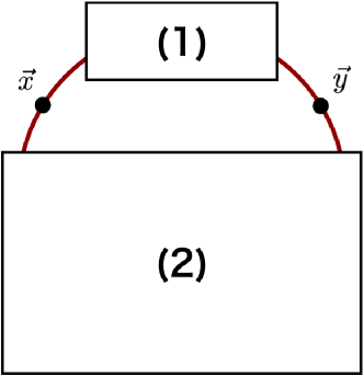
Refer to caption
Refer to caption
Figure 39: Illustration for why the single-bubble contribution arises in spite of the spherical symmetry of a single bubble. In this figure we show the envelope case and set tx=tysubscript𝑡𝑥subscript𝑡𝑦t_{x}=t_{y}. Same figure as in Ref. [85].

References