Localization in random bipartite graphs: numerical and empirical study

Abstract

We investigate adjacency matrices of bipartite graphs with power-law degree distribution. Motivation for this study is twofold. First, vibrational states in granular matter and jammed sphere packings; second, graphs encoding social interaction, especially electronic commerce. We establish the position of the mobility edge, and show that it strongly depends on the power in the degree distribution and on the ratio of the sizes of the two parts of the bipartite graph. At the jamming threshold, where the two parts have the same size, localization vanishes. We found that the multifractal spectrum is non-trivial in the delocalized phase, but still near the mobility edge. We also study an empirical bipartite graph, namely the Amazon reviewer-item network. We found that in this specific graph mobility edge disappears and we draw a conclusion from this fact regarding earlier empirical studies of the Amazon network.

I Introduction

Localization of eigenvectors is a phenomenon common to disordered systems. Since the pioneering work of P. W. Anderson anderson_58 , very large amount of knowledge was accumulated abrahams_10 ; lee_ram_85 ; kra_mcki_93 ; eve_mir_08 , yet rigorous answers are scarce ku_sou_83 ; stollmann_01 . Mostly we must rely on qualitative approaches abr_and_lic_ram_79 , analytical approximations based on diagrammatic methods vol_wol_80 ; suslov_95 ; jan_kol_05 , replica trick wegner_79a or supersymmetry efetov_83 , often using Bethe lattice as simplified geometry ab_an_tho_73 ; ab_tho_74 ; log_wol_85 ; ant_eco_77 ; gir_jon_80 ; efetov_90 ; mi_fyo_91 . Often the “brute force” numerical approaches lead to most reliable answers markos_06 ; mon_gar_10 .

Here we look at localization on random graphs bollobas_85 . We investigate the eigenvalues and eigenvectors of the adjacency matrix, which encodes the structure of the graph. Therefore, the disorder is purely off-diagonal, in contrast with e. g. the model of a quantum particle in random potential.

There are numerous motivations for studying spectra and localization in random graphs. Obviously, topologically disordered materials, like glasses, are common and investigation of their electronic and vibrational spectra has high practical relevance. Random graphs are a natural choice for modeling these structures. In the tight-binding approximation, the Hamiltonian of an electron in such structure composed of atoms of the same type (like a metallic glass) is proportional to the adjacency matrix of the graph. Hence the motivation for the study of spectral properties of adjacency matrices of random graphs.

As another example, granular materials ja_na_be_96a exhibit highly complex distribution of internal stress, often described in terms of force chains (see e. g. maj_beh_05 ). Sound propagates mainly along these chains ji_ca_ve_99 ; owe_dan_11 ; bas_owe_dan_por_12 , so we can make an abstract model of a granular matter in terms of a (random) graph representing the force chains. Vibrational states of the granular material then correspond to eigenstates of the Laplacian defined on the graph. Unusual behavior of low-energy vibrations in non-crystalline solids leads to anomalous thermal conductivity in such materials zel_poh_71 , which founds close analogy also in granular materials xu_vit_wya_liu_nag_09 .

Interestingly, the physics of glasses and granulars found recently a common ground in terms of the jamming transition ca_wi_bou_cla_98b ; liu_nag_10 ; liu_nag_saa_wya_11 ; tor_sti_10 . Packing of hard spheres is an extremely complex problem with ramifications in various disciplines ast_wea_08 ; con_slo_99 . Jamming transition occurs when average number of contacts is just sufficient for mechanical stability. Recently a model was proposed parisi_14 ; fra_par_16 ; fra_par_urb_zam_16 which relates sphere packing to combinatorial optimization nishimori_01 . In a typical setting, $N$ objects must satisfy $M$ constraints. This may be formulated as minimization problem for a Hamiltonian of $N$ variables, composed from $M$ additive terms. In a graph-theoretic language, the problem can be formulated in terms of a bipartite graph, with a set of $N$ variables on one side and set of $M$ constraints on the other side. When the Hamiltonian is expanded to harmonic approximation, its eigenmodes are related to the eigenvectors of the underlying bipartite graph. Hence the importance of studying bipartite graphs for the jamming problem.

Of course, the approach of Refs. parisi_14 ; fra_par_16 ; fra_par_urb_zam_16 is distant from real systems in the sense that they construct a kind of mean-field jamming transition, in which the number of contacts between spheres goes to infinity. However, such methodology proved already useful many times, especially in the theory of spin glasses nishimori_01 , which justifies its use also for the jamming problem. Formally it is manifested by replacing the real graph of contacts, which is embedded into three-dimensional Euclidean space, by a random graph which is effectively infinite-dimensional. We believe this also justifies the use of jamming terminology in the case of the random graphs used in this work. At the same time, we should keep in mind that graphs pertaining to realistic models of jamming should have quite narrow degree distribution. Therefore, in the context of our scale-free graphs we should rather speak of “abstract” of “generalized” jamming problem. In this sense we can speak of jamming transition in any bipartite graph.

However, our immediate motivation comes from the study of bipartite random graphs that naturally occur in electronic commerce. They belong to a broader class of scale-free graphs (i. e. those with power-law degree distribution) alb_bar_01 . At this point let us make just brief remark that related problems were also investigated in the field of correlation matrices la_ci_bou_po_99 ; ple_gop_ros_am_sta_99 ; ciz_bou_94 ; bur_jur_now_04 .

We already studied several electronic-commerce networks in the past sla_kon_10 ; slanina_12a ; slanina_14 . Here we shall reexamine the Amazon network sla_kon_10 . It is a bipartite graph of reviewers on one side and items offered for sale on the other side. We found that the degree distribution follows a power law on both sides. Moreover, we found by diagonalization of the corresponding matrix that the localized eigenvectors carry non-trivial semantic information on the network. Indeed, we were able to clearly identify several groups of agents sharing the same interests. Therefore, we found a practical application of the study of localization in empirical networks. However, it would be highly desirable to have a model of such network, at least to provide certain benchmark as to density of eigenvalues and dependence of the inverse participation ration on eigenvalue. We propose a random bipartite graph with power-law degree distribution as a model of these empirical networks. Here we want to study how much the model reproduces the empirical data as to spectrum and localization properties.

For completeness we should also mention that localization was already used in extracting information from scale-free graphs, e. g. in Refs. sad_kal_hav_ber_05 ; zhu_yan_yin_li_08 ; jal_sol_vat_li_10 ; gir_geo_she_09 ; odor_14 .

So, the aim of this work is investigation of spectra and especially the localization in bipartite random graphs with power-law degree distribution (usually called scale-free graphs, although this term is somewhat misleading). A good deal of information was already obtained on the spectra of scale-free graphs. To cite just a few articles, see far_der_bar_vic_01 ; goh_kah_kim_01b ; dor_gol_men_sam_03 . The most important finding is that the power-law degree distribution induces a power-law tail in the density of eigenvalues. This is found generally, irrespective of the specific model used for the scale-free graph.

From the mathematical point of view, spectra of random graphs are just spectra of a special type of random sparse matrices. Analytical approaches exist for the density of eigenvalues, using the replica trick rod_bra_88 ; sem_cug_02 ; rod_aus_kah_kim_05 ; nag_rod_08 or cavity approach ciz_bou_94 ; cav_gia_par_99 ; kuhn_08 (we proved that these two methods are strictly equivalent in slanina_11 ), or, alternatively, by mapping on a supersymmetric Hamiltonian rod_ded_90 ; fyo_mir_91 ; fyo_mir_91a .

Both replica trick and cavity method provide a ground for systematic analytic approximations, like effective-medium and single-defect approximations, which grasp essential features of the spectrum, like in Refs. rod_bra_88 ; bi_mo_99 ; sem_cug_02 ; slanina_11 . Of course, the cavity equations can be also solved by brute force using numerical population algorithms ciz_bou_94 ; cav_gia_par_99 ; cil_gri_mar_par_ver_05 ; kuhn_08 ; rod_cas_kuh_tak_08 ; met_ner_bol_10 ; bir_sem_tar_10 ; mon_gar_11 ; kuh_mou_11 ; kuhn_16 .

On the contrary, it is much harder to find similar analytical approximations to describe localization. Some of the difficulties encountered in attempts to find analytical approximations were investigated by us earlier slanina_12b . Therefore, numerical solution of the cavity equations is usually used as a reliable method ab_an_tho_73 ; ab_tho_74 ; cav_gia_par_99 ; cil_gri_mar_par_ver_05 ; met_ner_bol_10 . Of course, it is always possible to pursue the study by direct numerical diagonalization of sample random graphs evangelou_83 ; evangelou_92 ; eva_eco_92 ; ciz_bou_94 ; bi_mo_99 ; bir_sem_tar_10 ; mon_gar_11 ; slanina_12b ; bir_tei_tar_12 ; tik_mir_skv_16 . We shall resort to the latter approach here.

In our previous work we investigated localization on Erdős-Rényi random graphs and on random regular graphs slanina_12b . As we already hinted above, here we turn to localization on bipartite graphs. Spectra of such graphs, maybe under various disguises, were already studied earlier nag_tan_07 ; kho_rod_97 ; slanina_11 . We took inspiration from the work nagao_13 , where the spectrum of a scale-free bipartite graph was studied by replica approach within the effective-medium approximation. The structure of the graphs we shall construct will follow the algorithm of Goh et al. goh_kah_kim_01a . This is a natural generalization of the Erdős-Rényi graph ensemble to the case of non-uniform probabilities of placing edges between vertices. Spectra of these graphs were studied in Ref. rod_aus_kah_kim_05 and the generalization to bipartite graphs was investigated in the already mentioned Ref. nagao_13 . Our immediate aim is to add the aspect of localization to these studies.

II Scale-free bipartite graph

II.1 Relevance of the adjacency matrix

We shall deal with localization due to topological disorder, rather than random on-site potential. In the language of an electron moving in a random lattice represented by a graph $G$, we start with a general tight-binding Hamiltonian

$$H=\sum_{i}\epsilon_{i}|i\rangle\langle i|+\sum_{i<j}t_{ij}(|i\rangle\langle j|+|j\rangle\langle i|)$$ (1)

with on-site energies $\epsilon_{i}$ and hopping terms $t_{ij}$ connecting vertices $i$ and $j$ of the graph. Then we make a special choice relevant to our case, namely all diagonal elements equal (and without loss of generality they may be all zero) and hopping terms having value $t_{ij}=t$ if $(i,j)$ is an edge in the graph $G$ and $t_{ij}=0$ otherwise. Such situation occurs e. g. in metallic glasses. Indeed, all atoms are equal but the local structure may change from one site to another. Then, the Hamiltonian of the particle is proportional to the adjacency matrix of the graph $G$. Again, setting the proportionality constant $t=1$ just fixes the energy scale. Therefore, all essential information is obtained in the spectrum and eigenvectors of the adjacency matrix of the graph.

On the other hand, in the study of vibration states of glasses and granular matter we need to diagonalize the matrix representing the Laplacian on the graph. However, when we study the localization on random graphs, there is a disadvantage in using the Laplacian. Indeed, we want to separate the effect of on-site disorder (random atomic energy in tight-binding electronic Hamiltonian or random atomic mass in a model of vibrations) from the effect of random graph topology. In the Laplacian, this two effects are mixed, because diagonal element is related to the degree of the node in the graph. This aspect makes the analysis less transparent. Therefore, we prefer to study the spectrum of adjacency matrix, where on-site disorder is totally absent.

The third reason for studying adjacency matrix lies in our previous empirical study of Amazon network sla_kon_10 , which was done using adjacency matrix. Small communities in the network were successfully found by studying localization. To make comparison with a model random graph, adjacency matrix is studied also here.

II.2 Algorithm for graph creation

Now let us turn to our specific type of bipartite graph. The algorithm for creating instances of our random graph follows the original idea of Goh et al. goh_kah_kim_01a , further adapted by Nagao nagao_13 . We have two sets of vertices, the set A containing $N$, the set B containing $M$ vertices. We shall assume $N\leq M$. Among these vertices, $L$ edges are distributed, connecting always a vertex from A to a vertex from B. This way, a bipartite graph is created. The vertices are not statistically equivalent. The vertex $i$ from A is given an a priori probability $P_{Ai}$, similarly the vertices from $B$ will have probabilities $P_{Bj}$. To construct a scale-free graph, the probabilities will have the following power-law form

$$\begin{split}P_{Ai}&=\frac{i^{-\alpha_{A}}}{\sum_{l=1}^{N}l^{-\alpha_{A}}}\;,\;\;i=1,2,\ldots,N\\ P_{Bj}&=\frac{j^{-\alpha_{B}}}{\sum_{l=1}^{M}l^{-\alpha_{B}}}\;,\;\;j=1,2,\ldots,M\;.\end{split}$$ (2)

The edges are placed in the following way. In each step, a pair of vertices $(i,j)$ from A and B, respectively, is chosen randomly with probability $P_{Ai}P_{Bj}$. If an edge connecting $i$ and $j$ already exists, the choice is canceled and a new pair is randomly selected. (This may be repeated several times, if the graph is already rather dense, but as long as $L\leq NM$, a pair is eventually found.) Otherwise, a new edge is placed connecting $i$ and $j$. Repeating this procedure $L$ times we obtain a graph with exactly $L$ edges and there are no multiple edges. It was found that the cumulative degree distribution on the A side has a power-law tail $P^{>}(k)\sim k^{-\gamma}$, where $\gamma=1/\alpha_{A}$ for $\alpha_{A}<1$, while $\gamma=1$ for all $\alpha_{A}\geq 1$ goh_kah_kim_01a ; lee_goh_kah_kim_04 ; fle_sok_13 . By symmetry, analogous formulas hold for the degree distribution on the B side.

The structure of the graph is encoded in the adjacency matrix, which has, due to the bipartite character, the following form

$$R=\left(\begin{array}[]{cc}0&S\\ S^{T}&0\end{array}\right)$$ (3)

where $S$ is an $N\times M$ rectangular matrix. The spectrum of the matrix $R$ was studied using the replica method in Ref. nagao_13 . It was found that the density of eigenvalues has a power law tail which depends only on the greater of the two exponents $\alpha_{A}$, and $\alpha_{B}$. This suggests that it is sufficient to study graphs with both exponents equal, $\alpha_{A}=\alpha_{B}=\alpha$, which is what we shall assume in the following.

The matrix $R$ has size $(N+M)\times(N+M)$, which can be huge, as will be the case e. g. in the empirical data studied in the last section of this paper. However, essentially the same information on the spectrum and eigenvectors can be obtained from diagonalization of a smaller matrix $C=S\,S^{T}$ of size $N\times N$. Obviously, if $e$ is an eigenvector of $C$ with eigenvalue $\lambda^{2}$, then $\left(\begin{array}[]{c}e\\ S^{T}e/\lambda\end{array}\right)$ is an eigenvector of $R$ with eigenvalue $\lambda$ (see Appendix B, if unclear). Choosing plus or minus sign of $\lambda$ we find that single eigenvector $e$ of matrix $C$ corresponds to just two independent eigenvectors of $R$. If we are interested only in localization on the A side, knowledge of eigenvectors of $C$ is just sufficient. If we needed also elements of the eigenvector on the B side, they can be reconstructed from the eigenvector $e$ of matrix $C$. Therefore, all computations in this article are for the matrix $C$.

Using the replica method, it was found that the power-law tail of the density of eigenvalues of the matrix $C$ is $\mathcal{D}(z)\sim z^{-1-\tau}$, where $\tau=1/\alpha$ nagao_13 . Note that the exponent for the density of eigenvalues is the same as the exponent for the degree distribution.

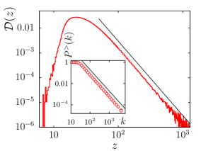
Figure 1: Density of eigenvalues for the graph with $\alpha=1/2$, $M/N=18$, $L/N=50$, and size $N=30000$. The straight line is the power $\propto z^{-3}$. In the inset, the cumulative degree distribution in the A set, for the same graph. The straight line is the power $\propto k^{-2}$.

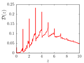
Figure 2: Detail of the density of eigenvalues for the graph with $\alpha=1/2$, $M/N=18$, $L/N=10$.

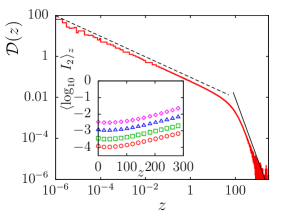
Figure 3: Density of eigenvalues for the graph with $\alpha=1/2$, $N=30000$, $M/N=1$, $L/N=50$. The straight lines are the powers $\propto z^{-1/2}$ (dashed) and $\propto z^{-3}$ (solid). In the inset, averaged logarithm of the inverse participation ratio for the graph with the same values of $\alpha$, $M/N$ and $L/N$ and sizes $N=30000$ ($\circ$), $N=10000$ ($\Box$), $N=3000$ ($\triangle$), and $N=1000$ ($\diamond$).

III Spectrum and localization

III.1 Sample preparation

Size dependence is the key to studying localization. Therefore, we create artificial sample graphs of four sizes, $N=10^{3}$, $N=3\cdot 10^{3}$, $N=10^{4}$, and $N=3\cdot 10^{4}$. For each size and each set of parameters $\alpha$, $M/N$, and $L/N$ we created certain number of independent samples of the random graph using the algorithm described in the previous section. The typical number of samples was about $2.5\cdot 10^{5}$, $2\cdot 10^{4}$, $10^{3}$, and $50$ for $N=10^{3}$, $N=3\cdot 10^{3}$, $N=10^{4}$, and $N=3\cdot 10^{4}$, respectively. For each sample, the matrix $C$ was diagonalized using the standard MATLAB library. The first thing we checked was the degree distribution of the graphs produced. We can see in the inset of Fig. 1 that our algorithm created a graph in full agreement with analytical predictions.

III.2 Density of eigenvalues

We show in Fig. 1 a typical example of the density of eigenvalues. The tail is characterized by a power-law decay, which again, as with the degree distribution, agrees very well with the analytic prediction. At the lower edge of the spectrum, the density of states falls off quickly and this is the region where we expect localization to occur. We can see that the density of eigenvalues is rather smooth there. This is typical for large enough $L/N$, i. e. for dense enough graphs. When the graph goes sparser, singularities accompanied by apparent delta-functions appear at integer eigenvalues, as can be seen in Fig. 2. The quality of the data do not allow to establish the form of the singularities. In Erdős-Rényi graphs it was found that the singularity at the center of the spectrum is logarithmic slanina_11 .So, by analogy we expect the singularities have logarithmic form also here. We do not know of any analytical theory which would describe this system of singularities sufficiently well. However, the mere presence of delta-functions can be understood by a simple consideration. Indeed, if $L/M<1$, as is the case in Fig. 2, a macroscopic fraction of vertices in the B set has degree $1$, i. e. does not provide a path from one A vertex to another one. This leads to creation of star-like components of the graph, where a single A vertex is linked to $m>0$ vertices from the set B, who themselves are not linked elsewhere. Such component contributes to the spectrum of the matrix $C$ by integer value $m$. The weight of thus created delta-function reflects the probability with which these stars appear in the bipartite graph. This mechanism is analogous to the appearance of delta-functions in the spectrum of Erdős-Rényi graphs, as shown numerically e. g. in evangelou_92 ; eva_eco_92 ; kuhn_08 ; kuh_mou_11 ; slanina_11 and analytically in bau_gol_01 ; golinelli_03 .

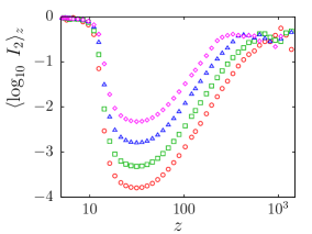
Figure 4: Averaged logarithm of the inverse participation ratio for the graph with $\alpha=1/2$, $M/N=18$ and $L/N=50$ and sizes $N=30000$ ($\circ$), $N=10000$ ($\Box$), $N=3000$ ($\triangle$), and $N=1000$ ($\diamond$).

For all $M/N>1$ the spectrum preserves the same overall character: there is a power-law tail at large $z$, with a power which depends only on $\alpha$, there is a bulk of the spectrum at intermediate $z$ and an area with low density of eigenvalues at small $z$. The latter area shrinks as $M/N$ approaches the critical value $M/N=1$, where another power-law dependence develops. We found that for $z\to 0$, the density of eigenvalues exhibits a singularity $\mathcal{D}(z)\sim z^{-1/2}$ for $M/N=1$, independently of the other parameters $L/N$ and $\alpha$. This is demonstrated in Fig. 3. In fact, this is exactly the behavior predicted for the case $M=N$ by the Marčenko-Pastur formula mar_pas_67 , which holds for $\alpha=0$ and $L/N\to\infty$.

In the interpretation of Refs. parisi_14 ; fra_par_16 ; fra_par_urb_zam_16 it corresponds to the critical point in the jamming transition. The $z^{-1/2}$ singularity translates into a flat density of vibrational states in jammed granular matter, as observed numerically her_sil_liu_nag_03 ; sil_liu_nag_05 as well as experimentally bri_dau_bir_bou_10 ; owe_dan_13 . Our result implies, that the singularity at the jamming threshold is universal, and holds for a broad range of random bipartite graphs.

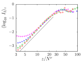
Figure 5: Detail of the averaged logarithm of the inverse participation ratio, versus the rescaled eigenvalue $z/N^{\nu}$, with $\nu=0.3$. The graph parameters are $\alpha=1/2$, $M/N=18$ and $L/N=50$ and sizes $N=30000$ ($\circ$), $N=10000$ ($\Box$), $N=3000$ ($\triangle$), and $N=1000$ ($\diamond$). The straight line is the dependence $3\log_{10}(z/N^{\nu})+\mathrm{const}$

III.3 Localization

As an indicator of localization we calculate the inverse participation ratio (IPR), defined as $I_{2}(z)=\sum_{i=1}^{N}e_{iz}^{4}$ for the eigenvector $e_{iz}$ corresponding to the eigenvalue $z$, normalized as $I_{1}(z)=\sum_{i=1}^{N}e_{iz}^{2}=1$ for all $z$. Localization is revealed in the behavior of IPR with increasing $N$, we therefore average the values of IPR for eigenvalues lying within an interval $(z_{-},z_{+})$ centered around $z=(z_{-}+z_{+})/2$. Numerically it is more convenient to average the logarithm of IPR, instead of IPR itself, although we suppose that at large enough $N$ both ways of averaging should lead to identical conclusions about localization. Therefore, we calculate the quantity

$$\langle\log_{10}\,I_{2}\rangle_{z}=\frac{1}{N_{z}}\sum_{z^{\prime}\in(z_{-},z_{+})}\log_{10}\,I_{q}(z^{\prime})$$ (4)

where $N_{z}$ is the number of eigenvalues inside the interval $(z_{-},z_{+})$. We use decadic logarithm for convenience. Localized and delocalized states differ in the dependence on the graph size for large $N$. Thus we have $\langle\log_{10}\,I_{2}\rangle_{z}\simeq c_{0}$ for $z$ in the region of localized states, while $\langle\log_{10}\,I_{2}\rangle_{z}\simeq c_{1}-\log_{10}N$ for $z$ in the region of delocalized states. Here $c_{0}$ and $c_{1}$ are constants independent of $N$.

The mobility edge $z_{\mathrm{mob}}$, i. e. the value of $z$ separating localized states on one side from delocalized ones on the other side, is extracted from the data by a procedure described in detail later.

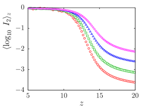
Figure 6: Detail of the averaged logarithm of the inverse participation ratio for the graph with $\alpha=1/2$, $M/N=18$ and $L/N=50$ and sizes $N=30000$ ($\circ$), $N=10000$ ($\Box$), $N=3000$ ($\triangle$), and $N=1000$ ($\diamond$).

We show in Fig. 4 typical behavior of the averaged log IPR for $\alpha>0$. We can see that the tail of the spectrum does not exhibit a clearly defined localized regime, contrary to the situation in Erdős-Rényi or random regular graphs slanina_12b . In the data, there is no clear mobility edge visible. Instead, the region of high IPR seems to shift farther in the tail when the graph size increases. In order to quantify this shift, we replotted the averaged log IPR in the rescaled variable $z/N^{\nu}$. We found that the best data collapse is achieved for the value of the exponent $\nu=0.3$. The rescaled plot is shown in Fig. 5. The observed data collapse suggest that in the tail the behavior of the inverse participation ratio is

$$\langle\log_{10}I_{2}\rangle_{z}=\Phi(z/N^{\nu})\;.$$ (5)

The scaling function $\Phi(x)$ exhibits two regimes, separated by a crossover at about $x_{\mathrm{cross}}\simeq 30$. For $x\gtrsim x_{\mathrm{cross}}$ the scaling function approaches a constant, $\Phi(x)\simeq C_{>}$, while for $x\lesssim x_{\mathrm{cross}}$ it approaches the function $\Phi(x)\simeq\mu\log_{10}(x)+C_{<}$ with coefficient $\mu=3$. The exact values of the constants $C_{<}$ and $C_{>}$ are irrelevant, but what counts are the values of the parameters $\mu$ and $\nu$. In fact, the observed scaling implies the behavior $\langle I_{2}\rangle\sim(z/N^{\nu})^{\mu}$. For fixed $z$ in the tail, but within the range $z\lesssim x_{\mathrm{cross}}N^{\nu}$ we have the dependence $\langle I_{2}\rangle\sim N^{-\nu\mu}$. The value of the product $\mu\nu$ is close but not quite equal to $1$, the exponent characteristic of extended states. It is not clear from the available data, whether the small difference is significant or it is due to statistical noise or it is a finite-size effect. We consider probable that the correct value of the product $\mu\nu$ is indeed $1$ but currently we are not able to prove it. At present stage we can formulate a hypothesis that all the states in the tail are extended for $z\lesssim x_{\mathrm{cross}}N^{\nu}$. This would mean that there is no mobility edge at the upper tail of the spectrum. However, the final verdict must be left for future.

The fact that localization occurs at small $z$ but, as it seems, does not appear at large $z$ is in contrast with the behavior of random correlation matrices, which in our language correspond to the value $\alpha=0$. In this case the probabilities $P_{Ai}$, $P_{Bj}$ are uniform, degree distribution of the graph is Poisson, the tail of the density of eigenvalues is steeper than any power and there is localized regime in the tail. Such graphs therefore exhibit two mobility edges, while for $\alpha>0$ the upper mobility edge vanishes, or, as we conjecture, is pushed far to infinity.

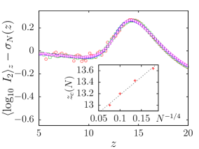
Figure 7: Data collapse of the averaged logarithm of the inverse participation ratio using the formulae (6) and (7). The data used are identical to those in Fig. 6. The meaning of the symbols is also the same. In the inset, extrapolation of the size-dependent estimates $z_{c}(N)$ to infinite size. This way the position of the mobility edge $z_{\mathrm{mob}}$ is established.

On the opposite side, for small $z$, the situation is much more clear-cut, as we observe unambiguous signs of localization. This fact is sufficiently evident in the detail shown in Fig. 6. For $z$ lower than about $9$ the value of log IPR does not depend on graph size. However, such estimate by bare inspection is not reliable enough. Let us now describe more sophisticated procedure for establishing the mobility edge $z_{\mathrm{mob}}$.

Below the mobility edge IPR scales with graph size as $\sim N^{0}$, while above the mobility edge the behavior is $\sim N^{-1}$. However, at finite $N$ the transition region has finite width in the variable $z$. This suggests the following scaling for the logarithm of IPR

$$\langle\log_{10}\,I_{2}\rangle_{z}=A(z)+\sigma_{N}(z)$$ (6)

where we denoted

$$\sigma_{N}(z)=\sigma\Big{(}\frac{z-z_{c}(N)}{w_{c}(N)}\Big{)}\,\log_{10}N\;.$$ (7)

In this expression $A(z)$ is a smooth function independent of $N$ and $\sigma(x)$ is a sigmoid-like function with asymptotic values $\sigma(x)\to 0$ for $x\to-\infty$ and $\sigma(x)\to-1$ for $x\to\infty$. The size-dependent parameters $z_{c}(N)$ and $w_{c}(N)$ are estimates of the position of the mobility edge and the width of the transition region for given graph size. The strategy for finding the mobility edge is to choose the sigmoid function and the set of parameters $z_{c}(N)$ and $w_{c}(N)$ so that the quantity $\langle\log_{10}\,I_{2}\rangle_{z}-\sigma_{N}(z)$ shows best data collapse for each four graphs sizes $N$ studied. We found that the precise shape of the sigmoid function is not crucial. Therefore, we used the simplest choice $\sigma(x)=-(1+\tanh(x))/2$. The optimization of the data collapse was performed using the simulated annealing procedure. An example of the result is given in Fig. 7, using the same data as shown in Fig. 6. We can see that the data collapse looks very good.

From thus obtained estimates $z_{c}(N)$ the mobility edge should be extrapolated in the limit $N\to\infty$. We found that the best fit of the size dependence provides the formula $z_{c}(N)=z_{\mathrm{mob}}+aN^{-1/4}$ with some constant $a$. An example of the fit is shown in the inset of Fig. 7. This way we obtain the mobility edge for all graphs studied. However, for a range of parameters the estimated mobility edge falls below zero, which means that localization is not observed at all. This happens typically for small values of $L/N$, i. e. if the graph is very sparse. An example of such situation is shown in Fig. 8, where $L/N=10$ and the mobility edge determined by the above procedure is negative, so we conclude that localization is absent. However, the presence of delta-functions at integer values of $z$ makes the analysis delicate and a more sophisticated procedure would be perhaps desirable.

The dependence of the critical value $z_{\mathrm{mob}}$ on graph parameters is shown in Figs. 9 and 10. First we can see that when the exponent $\alpha$ increases, the value of $z_{\mathrm{mob}}$ moves toward zero, until it disappears before $\alpha$ reaches the value $\alpha=1$.

Dependence on the parameter $L/N$ is shown in Fig. 10. We can observe more or less linear dependence on $L/N$, and vanishing of $z_{\mathrm{mob}}$ at certain value of this ratio, which is about $L/N\simeq 10$ for $\alpha=1/2$, $M/N=18$ and $L/N\simeq 15$ for $\alpha=3/4$, $M/N=18$. The dependence on the ratio $M/N$, as testified in the inset of Fig. 10, shows that the position of the mobility edge $z_{\mathrm{mob}}$ diminishes when the ratio $M/N$ approaches one.

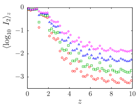
Figure 8: Detail of the averaged logarithm of the inverse participation ratio for the graph with $\alpha=1/2$, $M/N=18$ and $L/N=10$ and sizes $N=30000$ ($\circ$), $N=10000$ ($\Box$), $N=3000$ ($\triangle$), and $N=1000$ ($\diamond$).

In fact, it can be clearly observed that at the jamming threshold, $M/N=1$, the mobility edge disappears, as it is demonstrated in the inset of Fig. 3. This is consistent with the view of jamming threshold as a critical point. When we approach the critical point, the characteristic length scale diverges and as soon as it surpasses the localization length, localization is gone. At the same time we must be aware of the fact that jamming in granular matter occurs in three- or two-dimensional Euclidean space, while the random graph model of this article is not embedded in any Euclidean dimension. So, the qualitative considerations based on length scales surely cannot capture the full depth of the localization-versus-jamming problem.

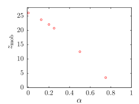
Figure 9: Dependence of the estimated position of the mobility edge on the parameter $\alpha$, for graphs with parameters $M/N=18$ and $L/N=50$.

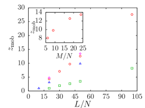
Figure 10: Dependence of the estimated position of the mobility edge on the parameter $L/N$ for $\alpha=1/2$ and $M/N=18$ ($\circ$), $\alpha=1/2$ and $M/N=24$ ($\diamond$), $\alpha=1/2$, and $M/N=9$ ($\triangle$), $\alpha=3/4$ and $M/N=18$ ($\Box$). In the inset, the dependence on $M/N$ for $\alpha=1/2$ and $L/N=50$.

A question which naturally occurs is how are the localized states related to other structural properties of the graph. Within the set of graphs investigated in this work we observed only quite strong correlation with the degree of nodes on which localization occurs. If $d_{i}$ is the degree of node $i$, we can average with respect to normalized eigenvector $e_{iz}$ corresponding to eigenvalue $z$ as $\langle d\rangle=\sum_{i}d_{i}e_{iz}^{2}$. We can see typical behavior in the lower part of the spectrum in Fig. 11. Clearly, the localized modes are centered at nodes with small degrees. We found that this is generic in the graphs studied here.

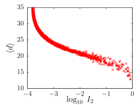
Figure 11: This graph shows correlation between average degree $\langle d\rangle$ and inverse participation ratio. Each point corresponds to a single eigenvector in the lower part of the spectrum, $z<30$. The parameters of the graph are $\alpha=0.5$, $N=30000$, $M/N=18$, $L/N=50$.

IV Multifractality

IV.1 Motivation

It is now well established that the eigenvectors at the localization transition exhibit multifractality (for review, see e. g. eve_mir_08 ). This peculiarity makes the localization transition more complex than usual critical phenomena in absence of quenched disorder. Recently there were studies hinting at multifractal statistics of eigenvectors also off criticality mon_gar_11 . In the context of many-body localization it was found that not only the critical, but also the extended states exhibit multifractality del_alt_kra_sca_14 . It is argued that this has decisive role in non-ergodicity of extended states. This topic is under hot debate currently tik_mir_skv_16 ; tik_mir_16 ; alt_iof_kra_16 . It seems that unusual multifractal behavior is related to the fact that these studies are carried on graphs containing randomness (Bethe lattices, random regular graphs, etc.) rather than in Euclidean space of dimensionality at most three. For example, the many-body localization occurs in Fock space, which has complex graph topology, usually approximated by locally tree-like graphs del_alt_kra_sca_14 . Therefore, we find natural to ask what are the multifractal properties of eigenvectors on random graphs of the specific type investigated here.

IV.2 Definitions

We shall use the notion of multifractality in a slightly modified sense, which we consider more appropriate for the problem at hand. To keep our language clear, let us introduce our definitions together with a few trivial examples.

The key quantities will be the moments of the eigenvectors $I_{q}(z)=\sum_{i=1}^{N}e_{iz}^{2q}$, where $q$ can assume any positive as well as negative value. For $q=2$ we recover the usual inverse participation ratio and for $q=1$ we have $I_{1}(z)=1$ for all eigenvalues $z$ due to normalization. in order to compare the values at different graph sizes, we should average over eigenvalues lying inside a narrow interval $(z_{-},z_{+})$ centered at a fixed value $z=(z_{-}+z_{+})/2$, exactly as it was when investigating the inverse participation ratio. So, $\langle I_{q}\rangle_{z}=\sum_{z^{\prime}\in(z_{-},z_{+})}I_{q}(z^{\prime})/N_{z}$, where $N_{z}$ is the number of eigenvalues inside the interval $(z_{-},z_{+})$.

When studying the multifractal properties of the eigenvectors, we suppose that the averages scale with the graph size as $\langle I_{q}\rangle_{z}\sim N^{-\zeta(q)}$, when $N\to\infty$. The function $\zeta(q)$ embodies the information on the multifractal character of the eigenvectors whose eigenvalues lie close to the point $z$. Let us see what the function $\zeta(q)$ looks like in a benchmark case, which is the Gaussian orthogonal ensemble. The distribution of eigenvector elements is Gaussian bro_flo_fre_mel_pan_won_81 ; la_ci_bou_po_99 (also called Porter-Thomas distribution in this context), which results in the following dependence on $N$ bro_flo_fre_mel_pan_won_81 ; eva_eco_90 . For $q>-1/2$ we have $\langle I_{q}\rangle_{z}\simeq N^{1-q}\;\frac{\Gamma(2q+1)}{2^{q}\,\Gamma(q+1)}$ and for $q<-1/2$ we have $\langle I_{q}\rangle_{z}\sim N^{-3q}$. Therefore, for GOE

$$\zeta(q)=\min(3q,q-1)\;.$$ (8)

Let us now look at the eigenvectors with eigenvalues close to a fixed value $z$ from a different perspective. We assume that the set of $N$ nodes can be divided into $G$ groups of sizes $N_{g}$, $g=1,2,\dots,G$, according to the scaling of the eigenvectors with the graph size $N$. We suppose that the elements of the eigenvectors scale like $|e_{i}|\simeq a_{g}N^{-h_{g}/2}$ for all $i$ within the group $g$, while the size of the group scales like $N_{g}\simeq b_{g}N^{d_{g}}$. The moments of the eigenvector then behave as $\langle I_{q}\rangle_{z}\simeq\sum_{g=1}^{G}a_{g}b_{g}\,N^{d_{g}-qh_{g}}$. For very large $N$ this sum is dominated by a single term with the maximum exponent, hence $\langle I_{q}\rangle_{z}\sim N^{-\zeta(q)}$, where

$$\zeta(q)=\min_{g}(qh_{g}-d_{q})\;.$$ (9)

Clearly, in a random graph the classification into such groups is only schematic. But we can introduce the classification in somewhat more formal way as follows. We fix a value $z$ and find an eigenvector with eigenvalue closest to $z$. Then we order the elements of the eigenvector in ascending order according to their modulus. Then, the smallest has index $1$ while the largest has index $N$. So we obtain a non-decreasing function. Then we numerically differentiate this function, so we obtain an estimate of probability density for the modulus of eigenvector elements. We can plot together such functions for all graphs sizes $N$ studied, while the value of $z$ remains fixed. It can be better done on logarithmic scale. Then we try to rescale the graphs so that they are shifted by $(h/2)\log N$ rightwards and $d\log N$ downwards. If all the graphs have a common intersection, we can conclude that we identified one group characterized by exponents $h$ and $d$. The coordinates of the intersection correspond to the parameters $\log a$ and $\log b$. Of course, we never do such procedure in reality, as we would need to check infinite number of possible combinations of $d$ and $h$. This description serves to the sole purpose to put the classification into groups on a more solid grounds.

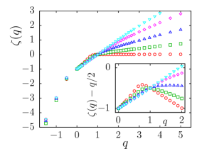
Figure 12: Scaling exponents for the eigenvector moments $\langle I_{q}\rangle_{z}$. The averages are made over intervals of width $1$ with midpoints at $z=8.5$ ($\circ$), $z=11.5$ ($\Box$), $z=12.5$ ($\triangle$), $z=13.5$ ($\diamond$), and $z=15.5$ ($\triangledown$). In the inset, detail of the same data. The term $q/2$ was subtracted just for better visibility of the nonlinear dependence on $q$.

We shall call the set of points $\{(h_{g},d_{g})|g=1,2,\ldots,G\}$ a multifractal spectrum of the eigenvectors. We can write it as a function $d(h)$, which can contain isolated points or continuous part, or both. Of course, it depends on the value $z$ around which the eigenvalues are taken. To see the point, let us consider eigenvectors of a complete graph. One of them (the ground state) is totally delocalized, i. e. $e_{i}=N^{-1/2}$ and all the others (excited states) are localized, one of them being $e_{1}=\sqrt{(N-1)/N}$, $e_{i}=-1/\sqrt{(N-1)N}$, $i>1$. So, the multifractal spectrum of the delocalized state consists of a single point $(1,1)$, while the localized states have a pair of points $\{(0,0),(2,1)\}$. In fact, the presence of the point $(0,0)$ is a fingerprint of localization, as it implies that whole weight of the eigenvector is carried by a set of sites which remains finite in the thermodynamic limit.

We can easily see by inspection that the multifractal spectrum which results in the GOE exponents (8) is also composed of just two points, $\{(1,1),(3,0)\}$. This is another example of a trivial multifractality. To have a non-trivial multifractal spectrum, or multifractality in proper sense, we need a continuous section in the function $d(h)$. We shall see later that it occurs close to the mobility edge.

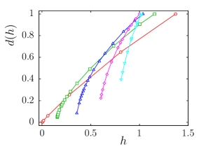
Figure 13: Multifractal spectrum obtained numerically from the data shown in Fig. 12, with the same meaning of the symbols.

IV.3 Numerical results

In our numerical studies, we shall compute the multifractal spectrum from the calculated exponents $\zeta(q)$ by a procedure which we call, for the sake of brevity, numerical inversion of the equation (9). The procedure goes as follows. We are looking for the function $d(h)$, which might be composed from a set of discrete points as well as continuous part(s). First we should guess the interval $I$ into which all values of $h$ should fall. As a first proxy for the function $d(h)$ we calculate, for each $h\in I$, the location and value of the minimum

$$v(h)=\min_{q}(qh-\zeta(q))=q_{\mathrm{m}}(h)h-\zeta(q_{\mathrm{m}}(h))\;.$$ (10)

It would be misleading to identify the function $v(h)$ with $d(h)$, as this would miss the fact that $d(h)$ contains isolated points. To cure this problem, we identify $d(h)=v(h)$ for each $h$ except such points where $q_{\mathrm{m}}(h)$ is locally constant, i. e. its first derivative with respect to $h$ exists and is zero. At such points the function $d(h)$ is undefined. Of course, numerically we discretize the interval $I$ and check if $q_{\mathrm{m}}(h)$ is constant by comparing its value at neighboring points.

Using this procedure we are respecting the fact that if the function $\zeta(q)$ contains a linear piece, such piece in its entirety corresponds to a single isolated point in the multifractal spectrum.

We calculated the exponents $\zeta(q)$ for $z$ above and slightly below the mobility edge. The density of states deep below the mobility edge is too small to provide reasonable statistical error for extracting the exponents from the averages $\langle I_{q}\rangle_{z}$. We show the results in Fig. 12. We observe that $\zeta(q)=0$ for $q>1$ below the mobility edge, as it should be in the localized state. Sufficiently far above the mobility edge we observe $\zeta(q)=q-1$ for all positive $q$, i. e. the GOE result. However, when we proceed from the mobility edge up, we depart from the localized behavior and approach the GOE limit rather slowly, indicating a relatively wide interval of eigenvalues with non-trivial behavior. The strong non-linearity of the function $\zeta(q)$ is stressed by plotting the detail in the inset of Fig. 12. Moreover, we should note that for negative exponents, more precisely for $q\leq-1/2$, the exponents obey the dependence $\zeta(q)=3q$ for all $z$, i. e. both in the localized and delocalized phase. This is in fact the same behavior as found also in GOE. So, this segment of the function $\zeta(q)$ is very robust and is not influenced by localization at all.

We further analyzed the exponents by numerically inverting the formula (9). The results are shown in Fig. 13. We can clearly see that the function $d(h)$ reaches maximum value $d(h)=1$, as it should. In the localized phase it contains also the point $(0,0)$, which is fully consistent with the considerations above. The most interesting part is the broad continuous section of he function $d(h)$, observed in the delocalized phase (note that the point $(0,0)$ is not included!), not too far from the mobility edge but certainly above it. This is the non-trivial part of the multifractal spectrum. The width of the continuous part shrinks as we go farther from the mobility edge, until it collapses onto the single point $(1,1)$, characteristic of GOE. We could speculate that the non-trivial multifractal spectrum in the delocalized phase describes analogous phenomenon as found in Ref. del_alt_kra_sca_14 . We should also note that the spectrum contains also the isolated point $(3,0)$, although it is not shown in the figure. This point originates from the behavior $\zeta(q)=3q$ for $q<-1/2$ which is shared with GOE always.

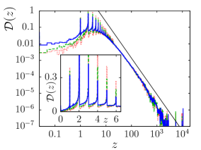
Figure 14: Density of eigenvalues obtained in the analysis of the empirical Amazon network. The size of the subset is $N=30000$ (solid line), $N=16000$ (dashed line), and $N=10000$ (dotted line). The straight line is the power $\propto z^{-2.2}$. In the inset, detail of the same data.

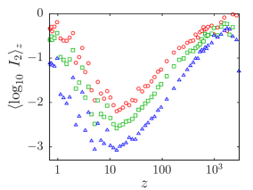
Figure 15: Averaged logarithm of the inverse participation
ratio, for the empirical Amazon network. The size of the subset is $N=30000$ ($\triangle$), $N=16000$ ($\Box$), and $N=10000$ ($\circ$).

V Empirical study

Now we turn to the analysis of an example of a bipartite scale-free graph taken from reality. We utilize the same data collection as already used in our previous work sla_kon_10 , so we only briefly describe them now. The data were collected in the year 2005, by automatic download from the server amazon.com. We were interested in the network connecting reviewers and items offered on Amazon. This is a bipartite graph, the set A being the collection of reviewers, the set B is the set of items, and the edges represent the reviews written. First we downloaded the list of all 1,714,512 reviewers present in the system at that time (now the list is hidden for its most part). The list was ordered by Amazon itself by relevance, which meant more or less by number of reviews written. Then, we downloaded systematically all reviews written by the first $10^{5}$ reviewers in this list. We found occasional duplicities in the data, and after cleaning them we obtained a graph composed of 99,622 reviewers and 645,056 items. These two sets were connected by 2,036,091 reviews.

In our study sla_kon_10 we looked at eigenvectors with largest IPR. We found that they identify small clusters within the network with clear semantic content, e. g. groups of publications about certain globally influential politician, another groups centered at popular musical bands etc. It would be tempting to make such an analysis automatically and rely on such computer-extracted data. However, the very question of reliability of these data is highly non-trivial. The first and essential question is whether the localized states are just casual products of the randomness of the underlying graph, or they are specific to this single empirical network. We are trying to contribute to solving this question first by comparing the Amazon network to a model random graph (which was done in the preceding sections). Second, we proceed by taking the graph representing the Amazon network as an input and trying to identify what is generic to this type of graph (which is what we are about to do in this section).

Therefore, in order to investigate systematic properties of this graph, rather than properties of this single empirical sample, we need an ensemble of random graphs with structure as close as possible to the given empirical sample. We prepare such random graphs by simply randomly selecting subgraphs of the empirical graph. So, smaller subgraphs were created by randomly choosing a set of $N$ reviewers and leaving only items connected to them. In our studies we used three sizes $N=10000$, $N=16000$, and $N=30000$. For each size we created 20 independent random realizations of the subset and averaged the density of eigenvalues and inverse participation ratio in the same way as it was done for the artificial graphs examined in the previous sections. Contrary to the artificial case, here we cannot choose neither the size $M$ nor the number of edges $L$ independently. These numbers also have some, although small, sample-to-sample fluctuation. On average, we found that $M/N\simeq 10$, for $N=30000$, $M/N\simeq 11.5$ for $N=16000$, and $M/N\simeq 13$ for $N=10000$. The ratio $L/N$ is, for all three sizes, $L/N\simeq 20$. As we have already shown in sla_kon_10 , the degree distribution is power-law on both the A and B sides, $P_{A,B}^{>}(k)\sim k^{-\gamma_{A,B}}$, but the exponents slightly differ: we found $\gamma_{A}\simeq 1.2$ and $\gamma_{B}\simeq 1.35$. The density of eigenvalues is shown in Fig. 14. We can observe the peaks at integer values of $z$ and the power-law tail. Comparing the spectra at increasing graph sizes we observe that the convergence is quite slow at small $z$, which is probably due to the fact that the ratio $M/N$ is not quite the same for all sizes, but decreases slightly when $N$ increases. However, the tail seems not to be affected, as it relies only on the power-law distribution of degrees. According to the general theory nagao_13 , only the smaller of the two exponents $\gamma_{A}$ and $\gamma_{B}$ is relevant for the tail of the eigenvalue density, so we expect that the exponent will be $\tau\simeq 1.2$. We can see in Fig. 14 that this is very well confirmed by the data.

In order to see if localized states occur in the spectrum, we plot in Fig. 16 the inverse participation ratio. In fact, no localization is observed in either low or high range of eigenvalues. At the upper tail, we observe qualitatively the same behavior as in the model graphs investigated in previous sections. There seems to be a crossover value $z_{\mathrm{cross}}$ and all states within the tail but with $z<z_{\mathrm{cross}}$ are extended. At the same time, $z_{\mathrm{cross}}$ seems to go to infinity with growing graph size. However, the data are too noisy to see this effect clearly. Neither the scaling like in (5) can be well observed with the present data. So, the absence of localization in the upper tail remains on the level of hypothesis, even more so than in the case of model graphs.

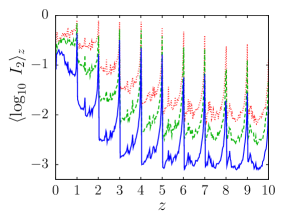
Figure 16: Detail of the data shown in Fig. 15. The size of the subset is $N=30000$ (solid line), $N=16000$ (dashed line), and $N=10000$ (dotted line).

Again, at low eigenvalues the situation is more clear. It is obvious that there is no region of localized states. The seemingly noisy behavior at small $z$ is in fact due to complex features, which are repeated at all sizes, just shifted downwards for increased $N$. This is clearly observable in the detail shown in Fig. 16. This figure also confirms that the localized phase is not present here. When we look at the behavior of the mobility edge in Fig. 9, we indeed expect vanishing of localization for the parameters relevant for the empirical data, which is, approximately, $M/N=10$, $L/N=20$, $\alpha=3/4$. We can finally conclude that both eigenvalue density and localization behavior of the empirical Amazon network is well reproduced by the model of Goh et al. goh_kah_kim_01a adapted for bipartite graphs in nagao_13 .

VI Conclusions

We investigated localization in bipartite graphs with power-law degree distribution. Localization is purely due to topological disorder. The main quantity to characterize localization was the inverse participation ratio, more precisely its dependence on the graph size. In comparison with the localization on Erdős-Rényi graphs, investigated by us earlier slanina_12b , there are several peculiarities. First, states at the upper tail of the spectrum behave differently, which is demonstrated both in power-law density of eigenvalues, and in localization properties. Based on our data, we conjecture that all the states which are in the upper tail but with eigenvalue below certain crossover value are extended; and, at the same time, the crossover value goes to infinity when the graph size increases. Our current data seem to support this hypothesis, but it would need better data to qualify it as proved.

At the lower edge of the spectrum, i. e. at eigenvalues close to zero, the region of localized states remains intact in a generic situation. However, the position of the mobility edge $z_{\mathrm{mob}}$ depends sensitively on the parameters of the model. At certain values of the parameters the critical value $z_{\mathrm{mob}}$ even drops to zero, which means that localization disappears. The general trend is that $z_{\mathrm{mob}}$ decreases with decreasing power in the degree distribution, with decreasing density of edges in the graph and also drops to zero when the sizes of the A and B sets (the two sides of the bipartite graph) becomes equal. The latter case is especially important, because it can be interpreted as jamming threshold in a man-field version of the sphere packing problem. This means that one critical point, the localization transition, is in conflict with another critical point, the jamming transition. We conjecture that this is due to competition between length scales characteristic for the two transitions. When one length scale prevails, the other critical point is concealed. There remains an important open question of how the disappearance of low-lying localized states will be reflected in heat conductance and sound transmission near and at the jamming threshold. To proceed in solving this question it would be necessary to adapt the model so that it is embedded in a three- or two-dimensional Euclidean space.

In the context of many-body localization bas_ale_alt_06 it is common to study level-spacing statistics as an indicator for localization instead of IPR oga_hus_07 . However, we found that this method is not very useful here, mainly due to very low density of states in the tail, where the localization occurs. So, we do not use this method here (see Appendix A for details).

We also analyzed multifractal properties of the eigenvectors. In some sense it is just deepening of the analysis based on the IPR. It includes the estimate of the position of the mobility edge as a by-product, as we identified the localized phase by the presence of the point $(0,0)$ in the multifractal spectrum. However, the finding we consider interesting is that the multifractal spectrum is non-trivial next to but in relatively broad range above the mobility edge. This may indicate that the eigenvectors are multifractal in the delocalized phase, as was found on random regular graphs in Ref. del_alt_kra_sca_14 or with a different approach in Ref. bir_tei_tar_12 , although these conclusions were questioned in tik_mir_skv_16 . In our view this phenomenon is connected with the topology of the random graph, more precisely with the distribution of loop lengths in the graph. Indeed, the graph is locally tree-like, typical loops having length $\ln N$. For computing spectra this is sufficient, but localization (or rather delocalization) is essentially non-local phenomenon and loops of length $\ln N$ cannot be considered large close to the critical region, where a typical length scale originating from localization competes with the typical length scale $\ln N$ originating from the topology. In finite-dimensionality lattices, distribution of loop lengths does not depend on system size, while in our random graph it does. Therefore, the scaling of the moments $I_{q}$ with graph size may be non-trivial in the delocalized phase. However, if this hypothesis is true, the range of observed multifractal states above mobility edge would ultimately shrink when system size grows, although for numerically accessible sizes the ultimate shrinking to a point may never be observable.

As a complement to the study of artificial bipartite graphs, we analyzed also one empirical bipartite graph, namely the network of reviewers and items on the amazon.com server. In our previous study sla_kon_10 we observed the scale-free nature of this graph and by extracting the most localized eigenvectors we found small communities with sensible semantic information. Here we wanted to check if the model of Goh et al. is useful also in describing the spectra of the graphs and properties of its eigenvectors. We found that indeed, the spectral and localization properties found in the empirical network are reproduced well within the Goh et al. model. This makes of it a useful benchmark in spectral studies of empirical networks, at least the electronic commerce networks investigated in sla_kon_10 . Most important conclusion is that in the empirical graph there should be no localization due to purely random geometry of the network. Therefore, the localized states found in sla_kon_10 are true outliers who bear specific information on this single instance of the empirical network. This is what we took as an assumption in sla_kon_10 and now we believe it is more firmly supported by the analysis of this work.

Appendix A Eigenvalue spacings

One of the key differences between localized and delocalized portion of the spectrum consists in the statistics of eigenvalue spacings. In GOE, it is very well approximated by the Wigner surmise $P_{\Delta\,\mathrm{GOE}}(x)=\frac{\pi}{2}\,xe^{-\pi\,x^{2}/4}$, where $x$ is the eigenvalue spacing normalized to its average value. If the eigenvalues were placed randomly according to a Poisson process, the distribution of normalized spacings would follow the exponential $P_{\Delta\,\mathrm{Poisson}}(x)=e^{-x}$. General expectation is that GOE result should hold in the delocalized regime, while localized states should correspond to Poisson level spacing distribution. Let us see now how this expectation is fulfilled in the case of our graphs.

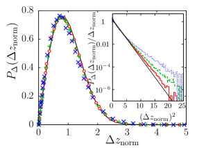
Figure 17: Distribution of eigenvalue spacings, for eigenvalues within the interval $(20,22)$ ($\circ$, solid line in inset), $(101,111)$ ($+$, dashed line in inset), and $(200,210)$ ($\times$, dotted line in inset). In the inset, the same data are plotted in rescaled form, to show the behavior in the tail. The parameters of the graph are $\alpha=1/2$, $M/N=18$, $L/N=50$ and size $N=1000$. The full line in the main plot and the straight line in the inset are the Wigner surmise $P_{\Delta}(\Delta z_{\mathrm{norm}})=(\pi\Delta z_{\mathrm{norm}}/2)\exp(-\pi\,(\Delta z_{\mathrm{norm}})^{2}/4)$.

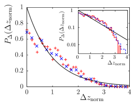
Figure 18: Distribution of eigenvalue spacings, for eigenvalues within the interval $(8,9)$. The parameters of the graph are $\alpha=0.5$, $M/N=18$, $L/N=50$ and size $N=1000$ ($+$, solid line in the inset), $N=3000$ ($\times$, dashed line in the inset). In the inset, the same data are plotted in logarithmic scale, to show the behavior in the tail. The full line in the main plot and the straight line in the inset is the dependence $\exp(-\Delta z_{\mathrm{norm}})$.

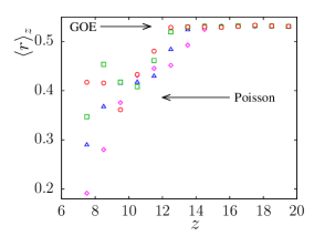
Figure 19: Spacing variation parameter, averaged over eigenvalues within the interval of width $1$ centered at $z$. The parameters of the graph are $\alpha=1/2$, $M/N=18$, $L/N=50$ and sizes $N=30000$ ($\circ$), $N=10000$ ($\Box$), $N=3000$ ($\triangle$), and $N=1000$ ($\diamond$). The horizontal arrows indicate the values which correspond to Gaussian orthogonal ensemble and to the Poisson placement of eigenvalues.

We calculated the distribution of eigenvalue spacings within several intervals across the spectrum. Taking interval $(z_{-},z_{+})$, we normalized the spacing between adjacent eigenvalues $z_{i+1}$, $z_{i}$ as $\Delta z_{\mathrm{norm}}=\frac{N_{z}}{z_{+}-z_{-}}(z_{i+1}-z_{i})$, where $N_{z}$ is the number of eigenvalues in the interval $(z_{-},z_{+})$. Such distributions can be directly compared with the GOE and/or Poisson result. This is done in Fig. 17 in the region well above the mobility edge and in the tail of the spectrum, and in Fig. 18 in the region slightly below the mobility edge. Deeper below the mobility edge the analysis is hindered by very small density of eigenvalues.

We can see that in the interval $(20,22)$, which lies above the mobility edge in the region of high density of eigenvalues, level spacings follow very well the GOE formula, confirming the status of delocalized eigenvectors. Farther in the tail, in the interval $(101,111)$, and even more in $(200,210)$, there are deviations from the Wigner surmise; large spacings are more probable than what GOE predicts. But the deviations are relatively small and do not harm the overall picture that all the delocalized regime is well characterized by GOE level spacings.

Below the mobility edge the conclusions are much less clear. The interval $(8,9)$ investigated here lies next to the mobility edge, while the localized states lying farther are too rare to obtain reasonable statistics of the level spacings. The distribution shown in Fig. 18 is certainly much closer to Poisson than to GOE, confirming the prediction that in localized regime GOE breaks down. However, we still cannot claim that the Poisson level spacing would make a good fit to the measured data. We assume that the difference from Poisson is due to closeness of the mobility edge. Farther away the spacing distribution is expected to correspond to the Poisson case much better.

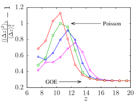
Figure 20: Relative variance of the eigenvalue spacing distribution within the interval of width $1$ centered at $z$. The parameters of the graph are $\alpha=1/2$, $M/N=18$, $L/N=50$ and sizes $N=30000$ ($\circ$), $N=10000$ ($\Box$), $N=3000$ ($\triangle$), and $N=1000$ ($\diamond$). The horizontal arrows indicate the values which correspond to Gaussian orthogonal ensemble and to the Poisson placement of eigenvalues.

Besides the full spacing distribution, there are aggregate parameters characterizing the spacing distribution in terms of a single number. The first one we use here is the ratio of two consecutive spacings $\Delta z_{i}=z_{i}-z_{i-1}$ and $\Delta z_{i+1}=z_{i+1}-z_{i}$ defined as oga_hus_07

$$r=\frac{\min(\Delta z_{i},\Delta z_{i+1})}{\max(\Delta z_{i},\Delta z_{i+1})}$$ (11)

and used frequently in the context of many-body localization bas_ale_alt_06 . This quantity was averaged over an interval of eigenvalues cantered at $z$, as it was done with inverse participation ratio. The average $\langle r\rangle_{z}$ should reflect the transition from GOE behavior, where $\langle r\rangle_{z}=0.529\ldots$, to Poisson behavior, where $\langle r\rangle_{z}=2\ln 2-1=0.386\ldots$ oga_hus_07 . We can see the results in Fig. 19. In the region far above the mobility edge we indeed observe that $\langle r\rangle_{z}$ settles at the GOE value. When we approach the mobility edge, $\langle r\rangle_{z}$ decreases, indicating the transition. However, the behavior below the mobility edge is ambiguous. The density of states is so small that the statistical fluctuations obscure the trend. Essentially the data are compatible with the idea that $\langle r\rangle_{z}$ approaches the Poisson value, but a firm statement cannot be done on the basis of current data. Certainly our results in no means prove that the spacing distribution in localized phase is Poisson, although the results neither prove the contrary.

Another single-valued indicator capable in principle to discern between GOE and Poisson regimes is the relative variance of the spacing distribution $\langle(\Delta z)^{2}\rangle_{z}/\langle\Delta z\rangle^{2}_{z}-1$. this quantity should be equal $1$ for Poisson and $4/\pi-1=0.2732\ldots$ for GOE spacing. We can see the numerical results for our graphs in Fig. 20. The behavior resembles that of the quantity $\langle r\rangle_{z}$. For $z$ sufficiently above the mobility edge, the relative variance is precisely at the GOE value. When we approach the mobility edge, the relative variance grows and at the mobility edge and below it decreases again. However, instead of approaching the Poisson limit, it is significantly smaller. This again casts some doubts at the hypothesis that in the localized phase the spacing distribution is Poisson. However, the discrepancy may also be due to finite size effects. As we can see in Fig. 20, the function does not seem to converge well in the range of graph sizes studied.

One should ask how to interpret these, rather negative, results.

Usually it is expected that the statistics corresponds to the Gaussian orthogonal ensemble in the delocalized regime, while it is Poisson in the localized one. The hypothesis on the delocalized state was fully confirmed in our studies, both by directly plotting the spacing distributions and by using aggregate quantities, like adjacent spacing ratio and relative variance. The deviations from GOE, if they exist at all, are small and restricted to the region of extremely large spacings, where finite size may play role.

On the other hand, the results in the localized regime are much less conclusive, mainly because the density of states is too low to obtain reliable results deep within the localized region. Below, but close to, the mobility edge, the spacing distribution is close to Poisson in the sense that it is purely decreasing function, but decreases more rapidly than an exponential, as would be expected for Poisson case. Also the aggregate quantities behave in a similar way; their value clearly departs from the GOE value when the mobility edge is crossed, but remains rather far from the value expected by Poisson spacing. We conclude that the analysis of eigenvalue spacing is not quite distinctive method for analyzing localization in this system. This is in contrast with the situation in e. g. random regular graphs studied by us in slanina_12b , where the Poisson distribution in localized phase was very well visible. We attribute this difference to the already mentioned scarcity of eigenvalues in localized region, which is characteristic for topological disorder (both in Erdős-Rényi graphs studied in slanina_12b and in bipartite graphs studied here). On the contrary, the random regular graphs are dominated by diagonal disorder (i. e. random potential) and the topological disorder, which is also present, has negligible effect. This has the effect that at in the localized phase there is still quite large density of eigenvalues, or even all the eigenstates are localized. This implies that reliable analysis of localization in topological disorder is much harder that in diagonal disorder.

The problem may be also formulated in the following way. Clearly, localization is an effect which cannot be in principle analyzed without a finite-size analysis. Indeed, localization means that the extent of the state does not increase when the extent of the whole system increases. Change in the level statistics seemingly avoids the necessity of both calculating IPR and making finite-size analysis. However, level statistics is only a secondary indicator. It is supposed to change abruptly when we are already working with infinite system. For finite systems we do not have any clue of how the spacing distribution should scale when the system size changes. The source of the difference between Poisson and GOE spacing distribution lies in the absence or presence of level repulsion in localized and delocalized states, respectively. When the density of eigenvalues is small, level repulsion can be hardly effective, thus masking the Poisson-to-GOE transition. This sheds some doubts on the use of aggregate quantities like the spacing ratio, but more detailed methodological analysis would be necessary here.

Appendix B Eigenvector of $R$ follows from eigenvector of $C$

Assumption is

$$Ce=\lambda^{2}e\;.$$ (12)

Denote

$$\bar{e}=\left(\begin{array}[]{c}e\\ S^{T}e/\lambda\end{array}\right)\;.$$ (13)

Therefore

$$\begin{split}R\bar{e}=\left(\begin{array}[]{cc}0&S\\ S^{T}&0\end{array}\right)\left(\begin{array}[]{c}e\\ S^{T}e/\lambda\end{array}\right)=\left(\begin{array}[]{c}SS^{T}e/\lambda\\ S^{T}e\end{array}\right)=\\ \left(\begin{array}[]{c}Ce/\lambda\\ \lambda S^{T}e/\lambda\end{array}\right)=\lambda\left(\begin{array}[]{c}e\\ S^{T}e/\lambda\end{array}\right)=\lambda\,\bar{e}\;.\end{split}$$ (14)

References

- (1) P. W. Anderson, Phys. Rev. 109, 1492 (1958).
- (2) E. Abrahams (Ed.), 50 Years of Anderson Localization (World Scientific, Singapore, 2010).
- (3) P. A. Lee and T. V. Ramakrishnan, Rev. Mod. Phys. 57, 287 (1985).
- (4) B. Kramer and A. MacKinnon, Rep. Prog. Phys. 56, 1469 (1993).
- (5) F. Evers and A. D. Mirlin, Rev. Mod. Phys. 80, 1355 (2008).
- (6) H. Kunz and B. Souillard, J. Physique Letters 44, L-411 (1983).
- (7) P. Stollmann, Caught by disorder. Bound states in Random Media (Birkhäuser, Boston, 2001).
- (8) E. Abrahams, P. W. Anderson, D. C. Licciardello, and T. V. Ramakrishnan, Phys. Rev. Lett. 42, 673 (1979).
- (9) D. Vollhardt and P. Wölfle, Phys. Rev. B 22, 4666 (1980).
- (10) I. M. Suslov, Sov. Phys. JETP 81, 925 (1995).
- (11) V. Janiš and J. Kolorenč, Phys. Rev. B 71, 033103 (2005).
- (12) F. J. Wegner, Phys. Rev. B 19, 783 (1979).
- (13) K. B. Efetov, Adv. Phys. 32, 53 (1983).
- (14) R. Abou-Chacra, P. W. Anderson, and D. J. Thouless, J. Phys. C: Solid State Phys. 6, 1734 (1973).
- (15) R. Abou-Chacra and D. J. Thouless, J. Phys. C: Solid State Phys. 7, 65 (1974).
- (16) D. E. Logan and P. G. Wolynes, Phys. Rev. B 31, 2437 (1985).
- (17) P. D. Antoniou and E. N. Economou, Phys. Rev. B 16, 3768 (1977).
- (18) S. M. Girvin and M. Jonson, Phys. Rev. B 22, 3583 (1980).
- (19) K. B. Efetov, Physica A 167, 119 (1990).
- (20) A. D. Mirlin and Y. V. Fyodorov, Nucl. Phys. B 366, 507 (1991).
- (21) P. Markoš, Acta Physica Slovaca 56, 561 (2006).
- (22) C. Monthus and T. Garel, Phys. Rev. B 81, 224208 (2010).
- (23) B. Bollobás, Random Graphs (Academic Press, London, 1985).
- (24) H. M. Jaeger, S. R. Nagel, and R. P. Behringer, Rev. Mod. Phys. 68, 1259 (1996).
- (25) T. S. Majmudar and R. P. Behringer, Nature 435, 1079 (2005).
- (26) X. Jia, C. Caroli, and B. Velicky, Phys. Rev. Lett. 82, 1863 (1999).
- (27) E. T. Owens and K. E. Daniels, EPL 94, 54005 (2011).
- (28) D. S. Bassett, E. T. Owens, K. E. Daniels, and M. A. Porter, Phys. Rev. E 86, 041306 (2012).
- (29) R. C. Zeller and R. O. Pohl, Phys. Rev. B 4, 2029 (1971).
- (30) N. Xu, V. Vitelli, M. Wyart, A. J. Liu, and S. R. Nagel, Phys. Rev. Lett. 102, 038001 (2009).
- (31) M. E. Cates, J. P. Wittmer, J.-P. Bouchaud, and P. Claudin, Phys. Rev. Lett. 81, 1841 (1998).
- (32) A. J. Liu and S. R. Nagel, Annu. Rev. Condens. Matter Phys. 1, 347 (2010).
- (33) A. J. Liu, S. R. Nagel, W. van Saarloos, and M. Wyart, in: Dynamical Heterogeneities in Glasses, Colloids, and Granular Media, eds. L. Berthier, G. Biroli, J.-P. Bouchaud, L. Cipelletti, and W. van Saarloos (Oxford UP, Oxford, 2011).
- (34) S. Torquato and F. H. Stillinger, Rev. Mod. Phys. 82, 2633 (2010).
- (35) T. Aste and D. Weaire, The Pursuit of Perfect Packing (Taylor and Francis, Boca Raton, 2008).
- (36) J. H. Conway and N. J. A. Sloane, Sphere Packings, Lattices and Groups (Springer, Berlin, 1999).
- (37) G. Parisi, arXiv:1401.4413.
- (38) S. Franz and G. Parisi, J. Phys. A: Math. Theor. 49, 145001 (2016).
- (39) S. Franz, G. Parisi, P. Urbani, and F. Zamponi, Proc. Nat. Acad. Sci. USA 112, 14539 (2015).
- (40) H. Nishimori, Statistical Physics of Spin Glasses and Information Processing (Clarendon Press, Oxford, 2001).
- (41) R. Albert and A.-L. Barabási, Rev. Mod. Phys. 74, 47 (2002).
- (42) L. Laloux, P. Cizeau, J.-P. Bouchaud, and M. Potters, Phys. Rev. Lett. 83, 1467 (1999).
- (43) V. Plerou, P. Gopikrishnan, B. Rosenow, L. A. N. Amaral, and H. E. Stanley, Phys. Rev. Lett. 83, 1471 (1999).
- (44) P. Cizeau and J.-P. Bouchaud, Phys. Rev. E 50, 1810 (1994).
- (45) Z. Burda, J. Jurkiewicz, M. A. Nowak, G. Papp, and I. Zahed, Physica A 343, 694 (2004).
- (46) F. Slanina and Z. Konopásek, Adv. Compl. Syst. 13, 699 (2010).
- (47) F. Slanina, Adv. Compl. Syst. 15, 1250053 (2012).
- (48) F. Slanina, Adv. Compl. Syst. 17, 1450002 (2014).
- (49) M. Sade, T. Kalisky, S. Havlin, and R. Berkovits, Phys. Rev. E 72, 066123 (2005).
- (50) G. Zhu, H. Yang, C. Yin, and B. Li, Phys. Rev. E 77, 066113 (2008).
- (51) S. Jalan, N. Solymosi, G. Vattay, and B. Li, Phys. Rev. E 81, 046118 (2010).
- (52) O. Giraud, B. Georgeot, and D. L. Shepelyansky, Phys. Rev. E 80, 026107 (2009).
- (53) G. Ódor, Phys. Rev. E 90, 032110 (2014).
- (54) I. J. Farkas, I. Derényi, A.-L. Barabási, and T. Vicsek, Phys. Rev. E 64, 026704 (2001).
- (55) K.-I. Goh, B. Kahng, and D. Kim, Phys. Rev. E 64, 051903 (2001).
- (56) S. N. Dorogovtsev, A. V. Goltsev, J. F. F. Mendes, and A. N. Samukhin, Phys. Rev. E 68, 046109 (2003).
- (57) G. J. Rodgers and A. J. Bray, Phys. Rev. B 37, 3557 (1988).
- (58) G. Semerjian and L. F. Cugliandolo, J. Phys. A: Math. Gen. 35, 4837 (2002).
- (59) G. J. Rodgers, K. Austin, B. Kahng, and D. Kim, J. Phys. A: Math. Gen. 38, 9431 (2005).
- (60) T. Nagao and G. J. Rodgers, J. Phys. A: Math. Theor. 41, 265002 (2008).
- (61) A. Cavagna, I. Giardina, and G. Parisi, Phys. Rev. Lett. 83, 108 (1999).
- (62) R. Kühn, J. Phys. A: Math. Theor. 41, 295002 (2008).
- (63) F. Slanina, Phys. Rev. E 83, 011118 (2011).
- (64) G. J. Rodgers and C. De Dominicis, J. Phys. A: Math. Gen. 23, 1567 (1990).
- (65) Y. V. Fyodorov and A. D. Mirlin, J. Phys. A: Math. Gen. 24, 2219 (1991).
- (66) Y. V. Fyodorov and A. D. Mirlin, Phys. Rev. Lett. 67, 2049 (1991).
- (67) G. Biroli and R. Monasson, J. Phys. A: Math. Gen. 32, L255 (1999).
- (68) S. Ciliberti, T. S. Grigera, V. Martín-Mayor, G. Parisi, and P. Verrocchio, Phys. Rev. B 71, 153104 (2005).
- (69) T. Rogers, I. Pérez Castillo, R. Kühn, and K. Takeda, Phys. Rev. E 78, 031116 (2008).
- (70) F. L. Metz, I. Neri, and D. Bollé, Phys. Rev. E 82, 031135 (2010).
- (71) G. Biroli, G. Semerjian, and M. Tarzia, Prog. Theor. Phys Suppl. 184, 187 (2010).
- (72) C. Monthus and T. Garel, J. Phys. A: Math. Theor. 44, 145001 (2011).
- (73) R. Kühn and J. van Mourik, J. Phys. A: Math. Theor. 44, 165205 (2011).
- (74) R. Kühn, Phys. Rev. E 93, 042110 (2016).
- (75) F. Slanina, Eur. Phys. J. B 85, 361 (2012).
- (76) S. N. Evangelou, Phys. Rev. B 27, 1397 (1983).
- (77) S. N. Evangelou, J. Stat. Phys. 69, 361 (1992).
- (78) S. N. Evangelou and E. N. Economou, Phys. Rev. Lett. 68, 361 (1992).
- (79) G. Biroli, A. C. Ribeiro-Teixeira, and M. Tarzia, arXiv:1211.7334.
- (80) K. S. Tikhonov, A. D. Mirlin, and M. A. Skvortsov, Phys. Rev. B 94, 220203 (2016).
- (81) T. Nagao and T. Tanaka, J. Phys. A: Math. Theor. 40, 4973 (2007).
- (82) A. Khorunzhy and G. J. Rodgers, J. Math. Phys. 38, 3300 (1997).
- (83) T. Nagao, J. Phys. A: Math. Theor. 46, 065003 (2013).
- (84) K.-I. Goh, B. Kahng, and D. Kim, Phys. Rev. Lett. 87, 278701 (2001).
- (85) D.-S. Lee, K.-I. Goh, B. Kahng, and D. Kim, Nucl. Phys. B 696, 351 (2004).
- (86) F. Flegel and I. M. Sokolov, Phys. Rev. E 87, 022806 (2013).
- (87) M. Bauer and O. Golinelli, J. Stat. Phys. 103, 301 (2001).
- (88) O. Golinelli, cond-mat/0301437.
- (89) V. A. Marčenko and L. A. Pastur, Math. USSR–Sbornik 1, 457 (1967).
- (90) C. S. O’Hern, L. E. Silbert, A. J. Liu, and S. R. Nagel, Phys. Rev. E 68, 011306 (2003).
- (91) L. E. Silbert, A. J. Liu, and S. R. Nagel, Phys. Rev. Lett. 95, 098301 (2005).
- (92) C. Brito, O. Dauchot, G, Biroli, and J.-P. Bouchaud, Soft Matter 6, 3013 (2010).
- (93) E. T. Owens and K. E. Daniels, Soft Matter 9, 1214 (2013).
- (94) A. De Luca, B. L. Altshuler, V. E. Kravtsov, and A. Scardicchio, Phys. Rev. Lett. 113, 046806 (2014).
- (95) K. S. Tikhonov and A. D. Mirlin, Phys. Rev. B 94, 184203 (2016).
- (96) B. L. Altshuler, L. B. Ioffe, and V. E. Kravtsov, arXiv:1610.00758.
- (97) T. A. Brody, J. Flores, J. B. French, P. A. Mello, A. Pandey, and S. S. M. Wong, Rev. Mod. Phys. 53, 385 (1981).
- (98) S. N. Evangelou and E. N. Economou, Phys. Lett. A 151, 345 (1990).
- (99) D. M. Basko, I. L. Aleiner, and B. L. Altshuler, Ann. Phys. 321, 1126 (2006).
- (100) V. Oganesyan and D. A. Huse, Phys. Rev. B 75, 155111 (2007).