An Interactive Greedy Approach to Group Sparsity in High Dimensions

Abstract

Sparsity learning with known grouping structure has received considerable attention due to wide modern applications in high-dimensional data analysis. Although advantages of using group information have been well-studied by shrinkage-based approaches, benefits of group sparsity have not been well-documented for greedy-type methods, which much limits our understanding and use of this important class of methods. In this paper, generalizing from a popular forward-backward greedy approach, we propose a new interactive greedy algorithm for group sparsity learning and prove that the proposed greedy-type algorithm attains the desired benefits of group sparsity under high dimensional settings. An estimation error bound refining other existing methods and a guarantee for group support recovery are also established simultaneously. In addition, we incorporate a general M-estimation framework and introduce an interactive feature to allow extra algorithm flexibility without compromise in theoretical properties. The promising use of our proposal is demonstrated through numerical evaluations including a real industrial application in human activity recognition at home. Supplementary materials for this article are available online.

Key Words: group Lasso, smart home, stepwise selection, variable selection, human activity recognition

1.   Introduction

High-dimensional data have become prevalent in many modern statistics and data mining applications. Given feature vectors $\mathbf{x}_{1},\mathbf{x}_{2},\cdots,\mathbf{x}_{n}\in\mathbb{R}^{p}$ and a sparse coefficient vector $\mathbf{w}^{*}\in\mathbb{R}^{p}$, consider a standard sparsity learning setting that $y_{i}\in\mathbb{R}$ ($i=1,\cdots,n$) is independently generated from some distribution $P_{\theta_{i}}$ depending on $\theta_{i}$ with linear relation $\theta_{i}=\mathbf{x}_{i}^{T}\mathbf{w}^{*}$, and that the feature dimension $p$ is much larger than $n$. Among various sparsity scenarios, we focus on group sparsity, where elements in $\mathbf{w}^{*}$ can be partitioned into known groups, and coefficients in each group are assumed to be either all zeros or all nonzeros. It is of primary interest to provide accurate estimation of $\mathbf{w}^{*}$ and identify the relevant groups. If ${\rm supp}(\mathbf{w}^{*})$ – the index set of nonzero elements in $\mathbf{w}^{*}$ – were known, the targeted problem can be naturally formulated through a criterion function $Q$ to find the “idealized” M-estimator

$$\bar{\mathbf{w}}=\operatorname*{argmin}_{\begin{subarray}{c}\mathbf{w}\in\mathbb{R}^{p}:\\ {\rm supp}(\mathbf{w}){\subset}{\rm supp}(\mathbf{w}^{*})\end{subarray}}\Bigl{\{}Q(\mathbf{w}):={\frac{1}{n}}\sum_{i=1}^{n}f_{i}(\mathbf{x}_{i}^{T}\mathbf{w})\Bigr{\}},$$ (1)

where $f_{i}(\cdot)$ is a given loss function determined by $y_{i}$. For example, under a standard linear model, we may choose least square loss $f_{i}(\theta_{i})=(y_{i}-\theta_{i})^{2}$; under generalized linear models (GLM) with canonical link (McCullagh and Nelder, 1989), we may use the negative log-likelihood. The estimator $\bar{\mathbf{w}}$ is “idealized” because ${\rm supp}(\mathbf{w}^{*})$ is not known a priori.

In certain real-world applications, the criterion function $Q$ may go beyond the standard setting of (1) when response $y_{i}$’s are not necessarily independent but the coefficient $\mathbf{w}$ has a known grouping structure requiring variable selection. In our theoretical and simulation studies (to be shown in Section 4 and Section 5), we will focus on the standard setting (with independent response). To allow extended real-world applications, the criterion function $Q$ can take more general forms (e.g., by setting $Q$ to be the negative log-likelihood), and our application example to be exihibited in Section 6 will fall under the extended setting (without independent response).

In standard sparsity learning, existing methods can be roughly categorized into shrinkage-type approaches (Tibshirani, 1996; Zou, 2006; Candes and Tao, 2005; Fan and Li, 2001; Zhang et al., 2010) and stepwise greedy-type approaches (Tropp, 2004; Zhang, 2011a; Ing and Lai, 2011). Following abundant work on sparsity learning, group sparsity has received considerable attention. Initially motivated from multi-level ANOVA models and additive models (Yuan and Lin, 2006), group sparsity learning and related studies has seen its use in many practical applications including genome wide association studies (e.g., Zhou et al., 2010), neuroimaging analysis (e.g., Jenatton et al., 2012, Jiao et al., 2017), multi-task learning (e.g., Lounici et al., 2011), actuarial risk segmentation (e.g., Qian et al., 2016), multi-view and manifold learning (e.g., Culp et al., 2018), sufficient dimension reduction and envelope models (e.g., Ding and Cook, 2018; Qian et al., 2018), among many others. There also exists another type of group sparsity for diversity selection (Kong et al., 2014; Yang et al., 2016; Huang and Liu, 2018) that emphasizes the diversity of selected features from groups. The benefits in estimation and inference using known grouping structure were also demonstrated through the celebrated group-Lasso methods (see, e.g., Huang and Zhang, 2010; Huang et al., 2012; Lounici et al., 2011; Mitra et al., 2016 and references therein).

In this paper, we propose a new group sparsity learning algorithm that generalizes from the practically very popular forward-backward greedy-type approach (Zhang, 2011a). We call this new algorithm Interactive Grouped Greedy Algorithm, or IGA for abbreviation.

As an increasingly popular application, the development of smart home management systems and associated techniques (e.g., for automatic life-logging, emergency alerts, energy control, etc.) has recently emerged as a promising applied research area. One of the fundamentally important challenges is how to automatically recognize human activities at homes. As a practical engineering solution, multiple pyroelectric sensors can be installed at home that capture binary signals in reaction to human motion. Due to cost and other related issues, the machine learning task is to identify only a small number of deployed sensors while maintaining reasonably high accuracy in human activity classification. Interestingly, this application can be formulated into a group sparsity learning problem since features and their coefficients that are associated with one sensor are naturally grouped together, without overlapping with any other sensor groups. By constructing the criterion function with negative log-likelihood under the extended setting, we have applied the proposed IGA algorithm for sensor (group) selection and will present the real data study in Section 6.

2.   Related Work and Contribution

To facilitate detailed exposition of our work’s contribution, in the following, we connect our work to existing literature in Section 2.1 before summarizing the contribution in Section 2.2.

2.1.   Related Work

In group sparsity learning, it is assumed that coefficient $\mathbf{w}=(w_{1},w_{2},\cdots,w_{p})\in\mathbb{R}^{p}$ can be partitioned into $m$ ($m\leq p$) non-overlapping groups with a known grouping structure, and we use $G=\{1,2,\cdots,m\}$ to denote the group index set. An important and fruitful line of work comes from shrinkage-based approaches. Extending from the Lasso (Tibshirani, 1996), the group Lasso has received considerable attention. Define the $\ell_{2,1}$ norm to be $\|\mathbf{w}\|_{G,1}:=\sum_{g\in G}\|\mathbf{w}_{g}\|$, where $\mathbf{w}_{g}$ is the sub-vector of $\mathbf{w}$ corresponding to group $g$ and $\lVert\cdot\rVert$ is the $\ell_{2}$ norm. Then the group Lasso imposes the $\ell_{2,1}$ norm penalty on the criterion function $Q$ with a tuning parameter $\alpha$ by

$$\min_{\mathbf{w}\in\mathbb{R}^{p}}Q(\mathbf{w})+{\alpha}\|\mathbf{w}\|_{G,1},$$ (2)

and its methods and algorithms have been studied under both linear model (Yuan and Lin, 2006) and GLM (Kim et al., 2006; Meier et al., 2008) settings. Mostly under linear model settings, theoretical properties of the group Lasso on both estimation and feature selection in high dimension have been investigated in, e.g., Nardi and Rinaldo (2008) and Wei and Huang (2010). Notably, under certain variants of group restricted isometry property (RIP, Candes and Tao, 2005) or restricted eigenvalue (RE, Bickel et al., 2009) conditions, the group Lasso was shown to be superior to the standard Lasso in estimation and prediction (Huang and Zhang, 2010; Lounici et al., 2011), thereby proving the benefits of group sparsity.

On the other hand, it is expected that the group Lasso inherits the same drawbacks of the Lasso, which include large estimation bias and relatively restrictive conditions on feature selection consistency (Fan and Li, 2001). Accordingly, various non-convex penalties such as SCAD (Fan and Li, 2001) and MCP (Zhang et al., 2010) as well as the adaptive Lasso type penalties (Zou, 2006; Zou and Zhang, 2009; Qian and Yang, 2013) were extended to allow incorporation of grouping structure and to replace the group Lasso penalty in (2) so that consistent group selection can be achieved with less restrictive conditions than the group Lasso (see, e.g., Huang et al., 2012; Jiao et al., 2017 and references therein).

Table 1: Comparison on the error bound $\|\hat{\mathbf{w}}-\mathbf{w}^{*}\|^{2}$ for sparse linear models. $\hat{\mathbf{w}}$ is the estimator by each algorithm. Assume each group has equal size $q=p/m$.

Algorithm	Error Bound $O_{p}(\cdot)$	Required sample size $\Omega(\cdot)$	Reference
Lasso	$\frac{k_{*}\log(p)}{n}$	$k_{*}\log(p)$	van de Geer et al. (2011)
Dantzig	$\frac{k_{*}\log(p)}{n}$	$k_{*}\log(p)$	Candes and Tao (2007)
Multistage Lasso	$\frac{k_{*}+\Delta_{2}\log(p)}{n}$	$k_{*}\log(p)$	Liu et al. (2012)
MCP	${\frac{k_{*}+\Delta_{1}\log(p)}{n}}$	$k_{*}\log(p)$	Zhao et al. (2017)
OMP	$\frac{k_{*}+\Delta_{1}\log(p)}{n}$	$k_{*}^{2}\log(p)$	Zhang (2009)
FoBa	${\frac{k_{*}+\Delta_{1}\log(p)}{n}}$	$k_{*}\log(p)$	Zhang (2011a)
Group Lasso	$\frac{k_{*}+\bar{k}\log({m})}{n}$	$k_{*}+\bar{k}\log({m})$	Huang and Zhang (2010)
Group OMP	$\frac{k_{*}\log(p)}{n}$	$k_{*}\log(p)$	Ben-Haim and Eldar (2011)
IGA	${\frac{k_{*}+{\Delta_{\text{IGA}}}\log({m})}{{n}}}$	$k_{*}+\bar{k}\log(m)$	Our proposal
$\Delta_{1}:={\left|\left\{i\in\text{supp}(\mathbf{w}^{*}):\leavevmode\nobreak\ |w^{*}_{i}|\leq\Omega\left(\sqrt{\log(p)\over n}\right)\right\}\right|}$
$\Delta_{2}:=k_{*}-\left|\left\{i:\leavevmode\nobreak\ i\text{-th largest element in}\leavevmode\nobreak\ |w_{i}^{*}|\geq\Omega{\left(\sqrt{\frac{(k_{*}-i)\log(p)}{n}}\right)}\right\}\right|$
$\Delta_{\text{IGA}}:=\left|{\left\{g\in G:\leavevmode\nobreak\ 0<\|\mathbf{w}^{*}_{g}\|\leq\Omega\left(\sqrt{{q+\log(m)\over n}}\right)\right\}}\right|$

Different from these shrinkage-based methods, the other main algorithm framework for group sparsity learning is the greedy-type methods. Greedy algorithms have received much attention in literature. For example, one of the representative algorithms is a forward greedy algorithm known as the orthogonal matching pursuit (OMP, Mallat and Zhang, 1993). Its feature selection consistency (Zhang, 2009) and prediction/estimation error bounds (Zhang, 2011b) have been established under an irrepresentable condition and a RIP condition, respectively. Backward elimination steps were incorporated to greedy algorithms in Zhang (2011a) to allow correction of mistakes made by forward steps (known as FoBa algorithm). This seminal work attained more refined estimation results than that of OMP and the Lasso by considering the delicate scenario of varying group signal strengths. Similar results on refined estimation error bound were also achieved by shrinkage-based methods with non-convex penalties (Zhao et al., 2017). Building on key understandings of the aforementioned greedy algorithms, much efforts were made to extend the OMP algorithms to handle group sparsity (Swirszcz et al., 2009; Ben-Haim and Eldar, 2011; Lozano et al., 2011). Although these group OMP algorithms have shown promising empirical performance, somewhat surprisingly, the explicitly justifiable benefits of group sparsity for greedy-type algorithms in terms of estimation convergence rate were yet to be rigorously established under a general setting.

Specifically, the $\ell_{2}$ estimation error bounds of some representative existing (group) sparsity learning methods under linear models are summarized in Table 1, and we will describe the improved convergence rate in the following Section 2.2. Here, ${\rm supp}(\mathbf{w})$ is the index set of nonzero elements in $\mathbf{w}$, and we define $\lVert\mathbf{w}\rVert_{0}$ to be the size of ${\rm supp}(\mathbf{w})$. Then given the true coefficient $\mathbf{w}^{*}$, $k_{*}=\lVert\mathbf{w}^{*}\rVert_{0}$ represents the total number of nonzero elements in $\mathbf{w}^{*}$. Also define the group $\ell_{0}$ norm $\|\mathbf{w}\|_{G,0}=\sum_{g\in G}I(\lVert\mathbf{w}_{g}\rVert>0)$ to be the number of groups in $G$ that corresponds to nonzero coefficients. Given $\mathbf{w}^{*}$ and any group $g\in G$, if all elements in $\mathbf{w}_{g}^{*}$ are zeros, then it is an irrelevant group to the response; otherwise, it is a relevant group. Then, $\bar{k}=\lVert\mathbf{w}^{*}\rVert_{G,0}$ represents the total number of relevant groups in the model. Let ${\Omega}\left(h_{1}(x)\right)$ be a function $h_{2}$ such that there exist two positive constants $M$ and $N$ with $N\leqslant M$, and we have $N|h_{1}(x)|\leqslant|h_{2}(x)|\leqslant M|h_{1}(x)|$ for sufficiently large $x$. We will also use the notations defined here for the rest of this paper.

2.2.   Our Contribution

The brief overview on related work above gives rise to three intriguing questions: (1) Can we devise a greedy-type algorithm that provides theoretically guaranteed benefits of group sparsity? Can we attain more refined estimation error bound than the group Lasso? (2) If so, is there any theoretical guarantee on correct support recovery of relevant groups? (3) Is our proposal practically relevant to modern industrial applications and easy to use for practitioners?

• As the main contribution of our work, the proposed IGA algorithm affirmatively addresses the three questions above simultaneously. Consider a group sparse linear model with even group size $q=p/m$ and define the squared $\ell_{2}$ estimation error $L_{2}(\hat{\mathbf{w}}):=\lVert\hat{\mathbf{w}}-\mathbf{w}^{*}\rVert^{2}$. Under a variant of the RIP condition, the IGA algorithm has $L_{2}(\hat{\mathbf{w}})=O_{p}{\left(\frac{k_{*}+{\Delta_{\text{IGA}}}\log({m})}{{n}}\right)}$, where $\Delta_{\text{IGA}}$ is the number of nonzero groups with relatively weak signals (see Table 1 for precise definition). This estimation error has convergence rate matching $O_{p}{\left(\frac{k_{*}+\bar{k}\log({m})}{n}\right)}$ under worst-case scenarios, confirming that our proposed greedy-type algorithm indeed gains the benefits of group sparsity as opposed to the slower convergence rate of $O_{p}(k_{*}\log(p)/n)$ for many standard sparsity learning methods. The desirable group support recovery property is also established for our proposal.

• Our proposal further develops a group forward-backward stepwise strategy by introducing extra algorithm flexibility to widen its applicability. First, it is worth noting that IGA is proposed under a general M-estimation framework and can apply to a broad class of criterion functions well beyond a standard linear model. In particular, under a GLM setting, we study the statistical properties of IGA for sparse logistic regression. We also demonstrate IGA’s promising applications on sensor selection for human activity recognition under an extended setting. Another interesting layer of flexibility comes from an adjustable human interaction parameter that can potentially give practitioners more freedom to incorporate their own domain knowledge in feature selection. Moreover, to further improve computational efficiency, we propose and study an algorithm variant called Gradient-based IGA, which, besides desirable statistical properties, enjoys much faster computation than the original IGA.

The rest of the paper is organized as follows. We introduce the proposed IGA algorithm, its heuristics, and the gradient-based IGA in Section 3. Section 4 provides the theoretical analysis with a general standard criterion function $Q(\mathbf{w})$. Sections 4.2 and 4.3 consider linear model and logistic regression as important special cases and show explicit estimation error bounds and group support recovery properties. Sections 5 and 6 show empirical studies using the IGA and its gradient-based variants in comparison with other state-of-the-art feature/group selection algorithms. All technical proofs and lemmas are left in the online Supplement.

3.   Our Proposal

The proposed IGA algorithm is an iterative stepwise greedy algorithm. At each iteration, a forward group selection step is performed, followed by a backward group elimination step. The forward step aims to identify one potentially useful group to be added to the estimator. This step typically identifies a set of candidate groups not selected yet, that can drive down the criterion function $Q(\mathbf{w})$ the most. The selected group is then added to the current group set for the next backward step. The backward step intends to fix mistakes made by early steps and eliminate redundant groups that do not significantly drive down $Q(\mathbf{w})$. The foward-backward iteration stops when no group can be selected in the forward step. Here, IGA is named interactive because in the forward step, rather than always choosing the top one group to reduce the criteria function most, we introduce an “interactive” discount parameter $\lambda$ that allows us to consider the top few candidate groups based on ranking and magnitude of criterion function reduction; a human operator is then allowed to select one group of his/her choice from these candidate groups, possibly based on domain knowledge or experience. In the following, we provide some intuitions and heuristics of IGA algorithm using a simple numerical example in Section 3.1, and then describe detailed algorithmic procedures in Section 3.2.

3.1.   A Heuristic Example

Different from a standard forward stepwise algorithm, IGA has both backward-elimination steps and an “interactive” discount parameter. To gain some intuitions and heuristics, consider a simple example with $m=5$ candidate groups, and each group $g$ ($g=1,\cdots,m$) contains 2 individual feature variables $X_{g,1}$ and $X_{g,2}$. Suppose that response $Y$ is generated by the first two groups as

$$Y=(X_{1,1}+X_{1,2})+(X_{2,1}+X_{2,2})+N(0,1).$$

Let $(X_{g,1},X_{g,2})$ all have independent standard normal distributions for $g=1,2,4,5$, and define for $g=3$ that

$$X_{3,1}=X_{1,1}+X_{1,2}+N(0,0.5)\text{ and }X_{3,2}=X_{2,1}+X_{2,2}+N(0,0.5).$$

Then although groups 1 and 2 are the true relevant groups, the forward selection will likely pick group 3 first as it can drive down the criterion function the most compared to the relevant groups individually. Indeed, we simulated $n=400$ data points and used the forward stepwise selection only (that is, always greedily add the group that gives smallest $Q(\mathbf{w})$), and as expected, the path of group selection was

$$\{3,\,2,\,1,\,5,\,4\},$$ (3)

and, cross validation (CV) selected the first three groups $\{3,1,2\}$ from the path. The group selection mistake made in the first step cannot be corrected and resulted in overfitting. To correct this mistake, IGA incorporates the backward selection technique that re-visits the selected groups to eliminate possibly redundant groups. Then with the forward-backward steps, the path of group selection in the simulation became

$$\{3,\,2,\,1,\,-3,\,5,\,4,\,3\},$$

where the first step mistake was corrected in the fourth step by eliminating group 3, and CV correctly selected groups $\{3,\,1,\,2,\,-3\}=\{1,2\}$ from the path.

The “interactive” parameter $\lambda$ ($0<\lambda\leq 1$; to be defined in Section 3.2) can also be potentially helpful as it allows the forward selection step to incorporate human operator’s expert opinion. For example, assume an expert gives his/her priority list $\mathcal{A}_{I}\subset G$. Then, in each forward step $k$, we will rank the criterion function values of each added group and consider an enlarged set of promising groups $\mathcal{A}_{\lambda}$ (as opposed to always considering the single top-ranked group), where the set size is related to $\lambda$. Then, if $\mathcal{A}_{I}\cap\mathcal{A}_{\lambda}\neq\emptyset$, we can follow both expert opinion $\mathcal{A}_{I}$ and forward selection top set $\mathcal{A}_{\lambda}$ to pick the group from $\mathcal{A}_{I}\cap\mathcal{A}_{\lambda}$ with smallest criterion function value; if $\mathcal{A}_{I}\cap\mathcal{A}_{\lambda}=\emptyset$, we simply pick the top group by forward selection and ignore $\mathcal{A}_{I}$. Specifically, in the numerical example above, suppose expert priority list $\mathcal{A}_{I}=\{1\}$ correctly includes group 1. Then with $\lambda=0.4$ (selected by CV), the forward stepwise algorithm gave the path

$$\{1,\,2,\,5,\,4,\,3\},$$ (4)

which correctly put $\{1,2\}$ in the solution path while pushing group 3 to later steps (as opposed to (3) that selected group 3 in the first step). Very different from the usual “offset” option in regression, not all groups in expert opinion list $\mathcal{A}_{I}$ has to be in the final selected model, and $\mathcal{A}_{I}$ is not necessarily all correct; interestingly, if we changed the expert opinion list to $\mathcal{A}_{I}=\{1,4\}$ in the simulation, where group 4 was incorrectly included in expert opinion list, the resulting path remained the same as (4), and CV gave the final selected group set $\{1,2\}$. In Section 4, we will show in theory that, with backward elimination, incorporating human expert opinions in our algorithm is safe in the sense that consistency properties still hold if $\lambda$ is not too small. We also repeated this simple experiement and observed similar results as described above. More experiment settings and simulation results are given in Section 5.

3.2.   IGA Algorithm

With the intuitions above, we are ready to present the detailed pseudo-code in Algorithm 1. Here, given any set $A$, let $|A|$ be its cardinality. Given a group $g\in G$, let $F_{g}\subset\{1,2,\cdots,p\}$ be the feature index set corresponding to group $g$; given a group set $S\subseteq G$, define $F_{S}=\cup_{g\in S}F_{g}$, which transforms the group index set $S$ to the corresponding feature index set. With the feature index set $F_{g}=\{i_{1},i_{2},\cdots,i_{\lvert F_{g}\rvert}\}\subset\{1,\cdots,p\}$, define $\mathbf{E}_{g}:=\left[\mathbf{e}_{i_{1}},\mathbf{e}_{i_{2}},\ldots,\mathbf{e}_{i_{|F_{g}|}}\right]$ to be a $p\times\lvert F_{g}\rvert$ matrix, where $\mathbf{e}_{i}\in\mathbb{R}^{p}$ is the unit vector whose $i$th element is 1 and all others are 0.

Algorithm 1 IGA algorithm.

0:  $\delta>0$, $0<\lambda\leq 1$

0:  $\mathbf{w}^{(k)}$

1:  $k=0,\mathbf{w}^{(k)}=0,G^{(0)}=\emptyset$

2:  while TRUE do

3:     if $\displaystyle{Q(\mathbf{w}^{(k)})-\min_{g\notin G^{(k)},\boldsymbol{\alpha}\in\mathbb{R}^{\lvert F_{g}\rvert}}Q(\mathbf{w}^{(k)}+\mathbf{E}_{g}\boldsymbol{\alpha})}<\delta$  then

4:         Break

5:     end if

6:      select an element as $g^{(k)}$ from the group set$\mathcal{A}_{\lambda}:=\{g\notin G^{(k)}\ |\ (Q(\mathbf{w}^{(k)})-\underset{\boldsymbol{\alpha}\in\mathbb{R}^{\lvert F_{g}\rvert}}{\operatorname{min}}\ Q(\mathbf{w}^{(k)}+\mathbf{E}_{g}\boldsymbol{\alpha}))\geqslant\lambda\ (Q(\mathbf{w})-\underset{\tilde{g}\notin G^{(k)},\,\boldsymbol{\alpha}\in\mathbb{R}^{\lvert F_{\tilde{g}}\rvert}}{\operatorname{min}}\ \ Q(\mathbf{w}^{(k)}+\mathbf{E}_{\tilde{g}}\boldsymbol{\alpha}))\}$

7:     $G^{(k+1)}={G^{(k)}\cup\{g^{(k)}\}}$

8:     $\mathbf{w}^{(k+1)}=\underset{\begin{subarray}{c}\mathbf{w}\in\mathbb{R}^{p}:\\ \textrm{supp }(\mathbf{w})\subset F_{G^{(k+1)}}\end{subarray}}{\operatorname{argmin}}\ Q(\mathbf{w})$

9:     $\delta^{(k+1)}=Q(\mathbf{w}^{(k)})-Q(\mathbf{w}^{(k+1)})$

10:     $k=k+1$

11:     while TRUE do

12:         if $\underset{g\in G^{(k)}}{\min}Q(\mathbf{w}^{(k)}-\mathbf{E}_{g}\mathbf{w}_{g}^{(k)})-Q(\mathbf{w}^{(k)})\geqslant\frac{\delta^{(k)}}{2}$ then

13:            Break

14:         end if

15:         $g^{(k)}=\underset{g\in G^{(k)}}{\operatorname{argmin}}\,Q(\mathbf{w}^{(k)}-\mathbf{E}_{g}\mathbf{w}_{g}^{(k)})$

16:         $k=k-1$

17:         $G^{(k)}=G^{(k+1)}{\setminus}\{g^{(k+1)}\}$

18:         $\mathbf{w}^{(k)}=\underset{\begin{subarray}{c}\mathbf{w}\in\mathbb{R}^{p}:\\ \textrm{supp }(\mathbf{w})\subset F_{G^{(k)}}\end{subarray}}{\operatorname{argmin}}\ Q(\mathbf{w})$

19:     end while

20:  end while

Specifically, we initialize the current set of groups $G^{(k)}$ as an empty set $G^{(k)}=\emptyset$ in Line 1, and then iteratively select and delete feature groups from $G^{(k)}$. Lines 3-5 provide the termination test: IGA terminates when no groups outside $G^{(k)}$ can decrease the criterion function $Q(\cdot)$ by a fixed threshold $\delta>0$. Line 6 is the key step for the forward group selection. First, we evaluate the quality of all groups outside of the current group set $G^{(k)}$ and, given a discount factor $\lambda\in(0,1]$, construct a candidate group set $\mathcal{A}_{\lambda}$ that includes all “good" groups. The human operator can then decide which group to select from $\mathcal{A}_{\lambda}$. Here the discount factor $\lambda$ determines the extent to which human interaction is desired. Bigger $\lambda$ typically gives smaller candidate group set and thereby less human involvement is allowed in group selection. In Lines 7-8, we recalculate the optimal coefficient of $\mathbf{w}$ supported on the updated group set. At the end of the forward step, we calculate the gain from this step as $\delta^{(k)}$ in Line 9, which will feed into the subsequent backward step.

In the backward step, we intend to check if any group in current group set $G^{(k)}$ becomes redundant considering that some previously selected groups may be less important after new groups join from the forward steps. In Lines 12-14, for each group in $G^{(k)}$, we calculate the difference between the criterion function value of the current group set and the function value with one group coefficients removed from the current pool. If the smallest difference is less than the threshold $\delta^{(k)}\over{2}$, in Lines 15-18, we remove the least significant group, update the current group set $G^{(k)}$ and re-calculate current estimator $\mathbf{w}^{(k)}$. This group elimination process continues until the function difference is less than $\delta^{(k)}\over{2}$, i.e., all remaining selected groups are considered to have significant contribution.

Algorithm 2 Gradient-based IGA algorithm.

0:  $\delta>0$, $0<\lambda\leq 1$

0:  $\mathbf{w}^{(k)}$

1:  $k=0,\mathbf{w}^{(k)}=0,F^{(0)}=\emptyset,G^{(0)}=\emptyset$

2:  while TRUE do

3:     if  $\|\nabla Q(\mathbf{w}^{(k)})\|_{G,\infty}<\varepsilon$  then

4:         Break

5:     end if

6:      select any $g^{(k)}\textrm{ in }\{g\notin G^{(k)}\ \ |\ \ \|\nabla_{g}Q(\mathbf{w}^{(k)})\|\geqslant\ \lambda\ \underset{\tilde{g}\notin G^{(k)}}{\operatorname{max}}\|\nabla_{\tilde{g}}Q(\mathbf{w}^{(k)})\|\}$

7:     $G^{(k+1)}={G^{(k)}\cup\{g^{(k)}\}}$

8:     $\mathbf{w}^{(k+1)}=\underset{\begin{subarray}{c}\mathbf{w}\in\mathbb{R}^{p}:\\ \textrm{supp }(\mathbf{w})\subset F_{G^{(k)}}\end{subarray}}{\operatorname{argmin}}\ Q(\mathbf{w})$

9:     $\delta^{(k+1)}=Q(\mathbf{w}^{(k)})-Q(\mathbf{w}^{(k+1)})$

10:     $k=k+1$

11:     while TRUE do

12:         if $\underset{g\in G^{(k)}}{\min}Q(\mathbf{w}^{(k)}-\mathbf{E}_{g}\mathbf{w}_{g}^{(k)})-Q(\mathbf{w}^{(k)})\geqslant\frac{\delta^{(k)}}{2}$ then

13:            Break

14:         end if

15:         $g^{(k)}=\underset{g\in G^{(k)}}{\operatorname{argmin}}\ Q(\mathbf{w}^{(k)}-\mathbf{E}_{g}\mathbf{w}_{g}^{(k)})$

16:         $k=k-1$

17:         $G^{(k)}=G^{(k+1)}{\setminus}\{g^{(k+1)}\}$

18:         $\mathbf{w}^{(k)}=\underset{\begin{subarray}{c}\mathbf{w}\in\mathbb{R}^{p}:\\ \textrm{supp }(\mathbf{w})\subset F_{G^{(k)}}\end{subarray}}{\operatorname{argmin}}\ Q(\mathbf{w})$

19:     end while

20:  end while

3.3.   Gradient-Based IGA Algorithm

Each forward step in Algorithm 1 requires to repeatedly perform optimization of the criterion functions (Lines 3 and Line 6) to evaluate quality across all candidate feature groups. It is interesting to note that these time-determining steps can be potentially replaced by using gradients of the criterion function $\nabla Q(\mathbf{w})$ so that we can avoid the repeated function optimization tasks and perform computation in a much more efficient way.

Specifically, given a threshold value $\varepsilon$ and a discount factor $0<\lambda\leq 1$, we can replace corresponding statements in Lines 3 and Line 6 with $\|\nabla Q(\mathbf{w}^{(k)})\|_{G,\infty}<\varepsilon$ and $\{g\notin G^{(k)}\ |\ \|\nabla_{g}Q(\mathbf{w}^{(k)})\|\geqslant\lambda\ \underset{\tilde{g}\notin G^{(k)}}{\operatorname{argmax}}\|\nabla_{\tilde{g}}Q(\mathbf{w}^{(k)})\|\}$, respectively, where $\nabla_{g}$ denotes the gradient with respective to group $g$, and $\|\mathbf{w}\|_{G,\infty}:=\max_{g\in G}\|\mathbf{w}_{g}\|$ represents the $\ell_{2,\infty}$ norm for any $\mathbf{w}\in\mathbb{R}^{p}$. Then we have a gradient-based version of the IGA algorithm and we call this variant Gradient-based IGA algorithm (or GIGA for brevity). The detailed procedures of GIGA algorithm are given in Algorithm 2. We will provide the theoretical properties of the GIGA algorithm in Section 4 and compare its computational performance with the original IGA algorithm in Section 5.

4.   Theoretical Results

This section provides theoretical analysis of Algorithm 1 and Algorithm 2. Using $\bar{\mathbf{w}}$ in (1) as a useful benchmark, we consider performance of IGA and GIGA estimator $\mathbf{w}^{(k)}$ under a general criterion function $Q$ in Section 4.1. Building on key results from this general setting in Section 4.1, we study sparse linear models in Section 4.2 and sparse logistic regression in Section 4.3 to provide valuable insights into coefficient estimation and group support recovery.

4.1.   A General Setting

We first introduce relevant definitions and assumptions regarding the setting on the general criterion function $Q(\cdot)$ in (1). Unless stated otherwise, we consider fixed designs in this section. Let $\bar{G}$ be the sparsest group set covering all nonzero elements in $\bar{\mathbf{w}}$ and let $\mathcal{D}\subset\mathbb{R}^{p}$ be a compact feasible region for $\mathbf{w}$. Given vectors $\mathbf{u},\mathbf{v}\in\mathbb{R}^{p}$, define $\langle\mathbf{u},\mathbf{v}\rangle=\mathbf{u}^{T}\mathbf{v}$ to be the inner product. Given any $F\subset\{1,\cdots,p\}$, define

$$\rho_{-}(F):= \inf_{\operatorname{supp}(\mathbf{u})\subset F,\mathbf{w}\in\mathcal{D}}\frac{Q(\mathbf{w}+\mathbf{u})-Q(\mathbf{w})-\langle\nabla Q(\mathbf{w}),\mathbf{u}\rangle}{{1\over 2}\|\mathbf{u}\|^{2}},$$ (5)

$$\rho_{+}(F):= \sup_{\operatorname{supp}(\mathbf{u})\subset F,\mathbf{w}\in\mathcal{D}}\frac{Q(\mathbf{w}+\mathbf{u})-Q(\mathbf{w})-\langle\nabla Q(\mathbf{w}),\mathbf{u}\rangle}{{\frac{1}{2}}\|\mathbf{u}\|^{2}}.$$ (6)

The restricted strongly convexity parameter and the restricted Lipschitz smoothness parameter (Huang and Zhang, 2010) are

$$\varphi_{-}(t)= \operatorname{inf}\{\rho_{-}(F_{S})\leavevmode\nobreak\ |\leavevmode\nobreak\ S\subset G,{|S|}\leqslant t\},$$ (7)

$$\varphi_{+}(t)= \operatorname{sup}\{\rho_{+}(F_{S})\leavevmode\nobreak\ |\leavevmode\nobreak\ S\subset G,{|S|}\leqslant t\},$$ (8)

respectively. Define the restricted condition number as $\kappa(t):=\frac{\varphi_{+}(t)}{\varphi_{-}(t)}$.

Assumption 1.

There exists a positive integer $s$ satisfying

$$\Omega(1)\leq\varphi_{-}(s)\leq\varphi_{+}(s)\leq\Omega(1),$$ (9)

$$s>\bar{k}+\frac{(\bar{k}+1)(\sqrt{\kappa(s)}+1)^{2}(\sqrt{2}\kappa(s))^{2}}{\lambda}.$$ (10)

In Assumption 1, (9) requires that $\varphi_{+}(s)$ and $\varphi_{-}(s)$ are upper bounded and bounded away from zero for large enough $n$. Given least square loss $f_{i}(z)={1\over 2}\|z-y_{i}\|^{2}$, the criterion function is $Q(\mathbf{w})={\frac{1}{2n}}\lVert\mathbf{y}-X\mathbf{w}\rVert^{2}$ with $\mathbf{y}\in\mathbb{R}^{n}$ being the response vector and $X$ being the $n\times p$ design matrix; then (9) becomes a variant of the group-RIP condition (Huang and Zhang, 2010). Indeed, (9) is satisfied if there is a constant $0<\eta<1$, such that

$$(1-\eta)\|{\mathbf{w}}\|^{2}\leqslant\frac{1}{{n}}\|X\mathbf{w}\|^{2}\leqslant(1+\eta)\|\mathbf{w}\|^{2}$$ (11)

for all $\|\mathbf{w}\|_{G,0}\leqslant s$. Similarly, under logistic regression with $f_{i}(z)=\log(1+\exp(-y_{i}z))$ ( $y_{i}\in\{-1,1\}$) and bounded covariates in $l_{2}$ norm, (9) is also satisfied with (11). The requirement in (10) of Assumption 1 is also mild. Note that $\kappa(s)$ is bounded if $Q(\mathbf{w})$ is a strongly convex function with bounded Lipschitzian gradient.

As mentioned, we assume the design matrix $X$ in the standard framework (1) is deterministic throughout the section. However, it is also noted that our results can be readily extended to random designs that satisfy Assumption 1 with high probability. For example, Lemma D.1 in Supplement D shows that Assumption 1 holds with high probability if $\mathbf{x}_{i}$’s are sub-Gaussian and the condition number of $\nabla^{2}f_{i}(\cdot)$ is bounded; least square function naturally satisfies this requirement; with bounded covariates, logistic regression also falls under this scenario.

Theorem 4.1.

Suppose Assumption 1 holds and $\delta=C_{\lambda}\|\nabla Q(\bar{\mathbf{w}})\|_{G,\infty}^{2}$, where $C_{\lambda}=\frac{8\varphi_{+}(1)}{\lambda\varphi_{-}^{2}(s)}$. Then IGA estimator $\mathbf{w}^{(k)}$ has the following properties:

• Algorithm 1 terminates at $k<s-\bar{k}$;

• $\|\bar{\mathbf{w}}-\mathbf{w}^{(k)}\|^{2}\leqslant\Omega\left(\lambda^{-1}\|\nabla Q(\bar{\mathbf{w}})\|_{G,\infty}^{2}\bar{\Delta}\right)$;

• $Q(\mathbf{w}^{(k)})-Q(\bar{\mathbf{w}})\leqslant\Omega\left(\lambda^{-1}\|\nabla Q(\bar{\mathbf{w}})\|_{G,\infty}^{2}\bar{\Delta}\right)$;

• $|G^{(k)}\setminus\bar{G}|+|\bar{G}\setminus G^{(k)}|\leqslant\Omega\left({\lambda^{-1}}\bar{\Delta}\right)$,

where $\bar{\Delta}:=\left|\{g\in\bar{G}:\|\bar{\mathbf{w}}_{g}\|<\Omega(\lambda^{-1}\|\nabla Q(\bar{\mathbf{w}})\|_{G,\infty})\}\right|$.

The first claim states that the algorithm terminates. Using $\bar{\mathbf{w}}$ as a benchmark, the second and third bounds provide the $\ell_{2}$ distance and the criterion function discrepancy of IGA estimator $\mathbf{w}^{(k)}$, respectively. The last bound describes the group feature selection difference between $\mathbf{w}^{(k)}$ and $\bar{\mathbf{w}}$. Note that all error bounds depend on $\bar{\Delta}$, which counts the number of “weak" signal groups among nonzero groups in $\bar{\mathbf{w}}$. If all nonzero groups are strong enough and $\bar{\Delta}$ turns out to be zero, then $\mathbf{w}^{(k)}$ becomes equivalent to $\bar{\mathbf{w}}$ and the original “idealized” problem (1) is exactly solved by Algorithm 1. Also, although the discount factor $\lambda$ slightly affects the error bound, if $\lambda$ is bounded away from zero, it would not change the order of error bounds above while allowing the extra flexibility in human expert participation.

Analysis of the gradient-based GIGA in Algorithm 2 provides theoretical results parallel to those for plain vanilla IGA in Algorithm 1. Indeed, as summarized in Theorem 4.2, with fixed $\lambda$, the rates of coefficient estimation and the group feature selection error bounds remain the same for GIGA as that of Theorem 4.1 for IGA.

Theorem 4.2.

Suppose Assumption 1 holds and $\varepsilon=\tilde{C}_{\lambda}\|\nabla Q(\bar{\mathbf{w}})\|_{G,\infty}$, where $\tilde{C}_{\lambda}=\frac{2\sqrt{2}\varphi_{+}(1)}{\lambda\varphi_{-}(s)}$. Then GIGA estimator $\mathbf{w}^{(k)}$ has the following properties:

• Algorithm 2 terminates at $k<s-\bar{k}$;

• $\|\bar{\mathbf{w}}-\mathbf{w}^{(k)}\|^{2}\leqslant\Omega\left(\lambda^{-2}\|\nabla Q(\bar{\mathbf{w}})\|_{G,\infty}^{2}\bar{\Delta}\right)$;

• $Q(\mathbf{w}^{(k)})-Q(\bar{\mathbf{w}})\leqslant\Omega\left(\lambda^{-2}\|\nabla Q(\bar{\mathbf{w}})\|_{G,\infty}^{2}\bar{\Delta}\right)$;

• $|G^{(k)}\setminus\bar{G}|+|\bar{G}\setminus G^{(k)}|\leqslant\Omega\left({\lambda^{-2}}\bar{\Delta}\right)$,

where $\bar{\Delta}=\left|\{g\in\bar{G}:\|\bar{\mathbf{w}}_{g}\|<\Omega(\lambda^{-1}\|\nabla Q(\bar{\mathbf{w}})\|_{G,\infty})\}\right|$.

Using the general results obtained in Theorem 4.1 and Theorem 4.2, we can demonstrate statistical properties of the IGA estimators under two special and important statistical model scenarios, which include sparse linear model in Section 4.2 and sparse logistic regression in Section 4.3. One interesting quantity from the theorems above is the gradient $\nabla Q(\bar{\mathbf{w}})$, and by construction, $\nabla_{\bar{G}}Q(\bar{\mathbf{w}})=\mathbf{0}$. In the following, we assume $\bar{\mathbf{w}}$ is the unique solution of $\nabla_{\bar{G}}Q(\mathbf{w})=\mathbf{0}$. We will focus on the cases that all $m$ groups have equal size $q=p/m$, although our analysis can allow arbitrary group sizes.

4.2.   Sparse Linear Model

Consider true model that response vector $\mathbf{y}\in\mathbb{R}^{n}$ is generated from $X\mathbf{w}^{*}+\boldsymbol{\varepsilon}$ with $\boldsymbol{\varepsilon}\sim N(\mathbf{0}_{n},I_{n})$. We use standard normal errors here, but our results can be easily generalized to sub-Gaussian errors. Suppose the columns of design matrix $X$ are normalized to $\sqrt{n}$ in $l_{2}$ norm. We consider analysis of IGA algorithm with the least square criterion function $Q(\mathbf{w})={\frac{1}{2n}}\lVert\mathbf{y}-X\mathbf{w}\rVert^{2}$. With $\nabla Q(\mathbf{w})=\frac{1}{n}X^{T}(X\mathbf{w}-\mathbf{y})$, the following Theorem 4.3 connects the gradients in Theorem 4.1 and Theorem 4.2 with the sparse linear model.

Theorem 4.3.

Suppose Assumption 1 holds. Then the true coefficient vector $\mathbf{w}^{\ast}$ and the benchmark estimator $\bar{\mathbf{w}}$ satisfies

$$\|\nabla Q(\mathbf{w}^{\ast})\|_{G,\infty}\leqslant O_{p}{\left(\sqrt{\frac{q+\log m}{n}}\right)}\quad\text{and}\quad\|\nabla Q(\bar{\mathbf{w}})\|_{G,\infty}\leqslant O_{p}{\left(\sqrt{\frac{q+\log m}{n}}\right)}.$$

In addition, we have $\max_{g\in\bar{G}}\lVert\bar{\mathbf{w}}_{g}-\mathbf{w}_{g}^{*}\rVert\leq O_{p}\Bigl{(}\sqrt{\frac{q+\log m}{n}}\Bigr{)}$.

Consequently, by combining Theorem 4.1 (or Theorem 4.2) and Theorem 4.3, we can obtain explicit IGA (or GIGA) estimation upper bounds for sparse linear model. In particular, both coefficient estimation and group support recovery can be shown in the following Theorem 4.4. Recall from the definition in Table 1 that $\Delta_{\text{IGA}}$ is the cardinality of the set of groups with relatively weak signals.

Theorem 4.4.

Suppose conditions of Theorem 4.1 (or Theorem 4.2) hold and $\lambda$ is bounded away from zero. Then IGA (or GIGA) estimator $\mathbf{w}^{(k)}$ for sparse linear model has following statistical properties:

• $L_{2}(\mathbf{w}^{(k)}):=\|\mathbf{w}^{(k)}-\mathbf{w}^{*}\|^{2}=O_{p}\Bigl{(}{k_{*}+\Delta_{\text{IGA}}\log m\over n}\Bigr{)}.$

• There is a constant $C>0$ (not depending on $n$) such that if $\min_{g\in\bar{G}}\lVert\mathbf{w}_{g}^{*}\rVert\geq C\sqrt{\frac{q+\log(m)}{n}}$, then group selection consistency holds that $P(G^{(k)}=\bar{G})\rightarrow 1$ as $n\rightarrow\infty$.

Interestingly, the estimation consistency in Theorem 4.4 indeed demonstrates the benefits of group sparsity in estimation convergence rate: the estimation error $L_{2}(\mathbf{w}^{(k)})$ is upper bounded by $O_{p}{\left({k_{*}+\bar{k}\log m\over n}\right)}$, which improves over the rate $O_{p}{\left(\frac{k_{*}\log(p)}{n}\right)}$ of standard sparsity. In addition, our results can be more refined than the group Lasso in the existence of relatively strong group signals. In particular, under the beta-min condition that coefficients of all $\bar{k}$ relevant groups have $\ell_{2}$-norm lower bounded by $\Omega{\left(\sqrt{{q+\log m\over n}}\right)}$, $L_{2}(\mathbf{w}^{(k)})$ is improved to $O_{p}(k_{*}/n)$ by removing an additive term $\bar{k}\log m/n$, which can be a substantial improvement in high-dimensional settings $m\gg n$ with relatively strong group signals; under the same conditions, Theorem 4.4 also shows that the IGA (or GIGA) estimator is consistent in group support recovery.

4.3.   Sparse Logistic Regression

We assume the sparse logistic regression setting here with binary response $y_{i}\in\{-1,\,1\}$ and $\mathbf{Pr}(y_{i}=1\,|\,\mathbf{x}_{i})=\frac{\exp(\mathbf{x}_{i}^{T}\mathbf{w}^{*})}{1+\exp(\mathbf{x}_{i}^{T}\mathbf{w}^{*})}$ for $1\leq i\leq n$. Then with the negative log-likelihood criterion function $Q(\mathbf{w})=\frac{1}{n}\sum_{i=1}^{n}\log(1+\exp(-y_{i}\mathbf{x}_{i}^{T}\mathbf{w}))$, the gradient is $\nabla Q(\mathbf{w})=\frac{1}{n}X^{T}\mathbf{h}(\mathbf{w})$, where $\mathbf{h}(\mathbf{w})=(h_{1}(\mathbf{w}),\cdots,h_{n}(\mathbf{w}))^{T}$ and $h_{i}(\mathbf{w})=\frac{-y_{i}}{1+\exp(y_{i}\mathbf{x}_{i}^{T}\mathbf{w})}$. Let $X_{g}$ and $X_{\bar{G}}$ be the design matrix corresponding to group $g$ ($1\leq g\leq m$) and group set $\bar{G}$, respectively. Define $n\times n$ diagonal matrix $W(\mathbf{w})=\mathrm{diag}(\nu_{1}(\mathbf{w}),\cdots,\nu_{n}(\mathbf{w}))$, where $\nu_{i}(\mathbf{w})=p_{i}(\mathbf{w})(1-p_{i}(\mathbf{w}))$ and $p_{i}(\mathbf{w})=\frac{\exp(\mathbf{x}_{i}^{T}\mathbf{w})}{1+\exp(\mathbf{x}_{i}^{T}\mathbf{w})}$. Set $W^{*}=W(\mathbf{w}^{*})$. We then consider the quantities $U_{1}=\lVert\frac{1}{n}X_{\bar{G}}^{T}X_{\bar{G}}\rVert$, $U_{2}=\lVert(\frac{1}{n}X_{\bar{G}}^{T}W^{*}X_{\bar{G}})^{-1}\rVert$ and $U_{3}=\max_{g\in G\backslash\bar{G}}\lVert\frac{1}{n}X_{g}^{T}W^{*}X_{\bar{G}}\rVert$. Variants of these quantities have been used to study properties of shrinkage-type approaches (e.g., Fan et al., 2014). We now connect the gradients in Theorem 4.1 and Theorem 4.2 with the sparse logistic regression through the following Theorem 4.5, which gives results similar to that of Theorem 4.3.

Theorem 4.5.

Suppose Assumption 1 holds. Assume $\bar{k}^{2}(q+\log m)=o(n)$ and quantities $U_{1}$, $U_{2}$, $U_{3}$ are upper bounded. Then we have

$$\|\nabla Q(\mathbf{w}^{\ast})\|_{G,\infty}\leqslant O_{p}{\left(\sqrt{\frac{q+\log m}{n}}\right)},\quad\|\nabla Q(\bar{\mathbf{w}})\|_{G,\infty}\leqslant O_{p}{\left(\sqrt{\frac{q+\log m}{n}}\right)},$$

and $\max_{g\in\bar{G}}\lVert\bar{\mathbf{w}}_{g}-\mathbf{w}_{g}^{*}\rVert\leq O_{p}\Bigl{(}\sqrt{\frac{q+\log m}{n}}\Bigr{)}$.

Combining Theorem 4.1 (or Theorem 4.2) and Theorem 4.5, we establish the IGA (or GIGA) estimator’s statistical properties in Theorem 4.6 for logistic regression. The conclusion similar to that of sparse linear model still holds here, which provides a refined estimation convergence rate. In particular, if all the relevant groups have relatively large signals, the coefficient estimation error can be improved to $O_{p}(k_{*}/n)$ and is consistent in group support recovery.

Theorem 4.6.

Suppose conditions of Theorem 4.1 (or Theorem 4.2) and Theorem 4.5 hold and $\lambda$ is bounded away from zero. Then IGA (or GIGA) estimator $\mathbf{w}^{(k)}$ under the logistic regression setting has following estimation and group selection properties:

• $\|\mathbf{w}^{(k)}-\mathbf{w}^{*}\|^{2}=O_{p}\Bigl{(}{k_{*}+\Delta_{\text{IGA}}\log m\over n}\Bigr{)}.$

• There is a constant $\tilde{C}>0$ (not depending on $n$) such that if $\min_{g\in\bar{G}}\lVert\mathbf{w}_{g}^{*}\rVert\geq\tilde{C}\sqrt{\frac{q+\log(m)}{n}}$, then $P(G^{(k)}=\bar{G})\rightarrow 1$ as $n\rightarrow\infty$.

5.   Simulation

In this section, we evaluate the performance of the proposed algorithms on simulation data. As illustrated in the heuristic example of Section 3.1, the forward selection and backward elimination scheme in IGA naturally provides a group selection path similar to the solution path of shrinkage-based methods like the group Lasso; correspondingly, rather than directly setting the parameter $\delta$ to determine the final model’s group sparsity level, we can equivalently generate a group selection path and choose the appropriate sparsity level $k$ from the path to estimate the final model. Without setting constraints on model’s sparsity level, we used ten-fold CV to automatically determine $k$ in the simulation.

Another parameter in IGA is the “interactive” parameter $\lambda$, which potentially allows help from human expert opinions. As illustrated in Section 3.1, if an expert provides a priority list $\mathcal{A}_{I}$, and $\mathcal{A}_{I}\cap\mathcal{A}_{\lambda}\neq\emptyset$ in the forward selection step, then IGA adds the group in $A_{I}\cap\mathcal{A}_{\lambda}$ that gives the smallest $Q(\mathbf{w})$; if $\mathcal{A}_{I}\cap\mathcal{A}_{\lambda}=\emptyset$ in the forward selection step, IGA adds the group in $\mathcal{A}_{\lambda}$ that gives the smallest $Q(\mathbf{w})$; if there is no expert opinion (or $\mathcal{A}_{I}=\emptyset$), simply set $\lambda=1$. Recall from Table 1 that $\bar{k}=\lVert\mathbf{w}^{*}\rVert_{G,0}$ is the total number of relevant groups in the true model. To mimic a more realistic scenario that expert opinion may contain both correct and incorrect components, $\mathcal{A}_{I}$ correctly contains $\lfloor\frac{3}{5}\bar{k}\rfloor$ of relevant groups and incorrectly contains an equal number of $\lfloor\frac{3}{5}\bar{k}\rfloor$ irrelevant groups throughout this simulation study. With $\mathcal{A}_{I}$, we used ten-fold CV to automatically select $(k,\lambda)$, and $\lambda$’s candidate values were $\{0.2,0.4,0.6,0.8,1.0\}$. To differentiate methods based on whether IGA uses $\mathcal{A}_{I}$, we denote the IGA algorithm that selected $\lambda$ with CV as “IGA-$\lambda$”, and denote the IGA algorithm with pre-specified $\lambda=1$ (that is, it ignored the interactive parameter and $\mathcal{A}_{I}$) as “IGA”.

In light of our previous theoretical understandings, to gauge the proposal’s numerical performance, we considered FoBa and the group Lasso as the representative benchmark methods and implemented them in MATLAB. Both methods have their own tuning parameters: the sparsity-level parameter of FoBa was tuned the same way as $k$ in IGA, but the known group structure was ignored; we also implemented the group Lasso by the accelerated proximal gradient descent (Beck and Teboulle, 2009) and used “warm start” to generate the solution path (that corresponds to a decreasing sequence of shrinkage tuning parameters; Friedman et al., 2010). Ten-fold CV was used to select tuning parameters for these benchmark methods.

Let $\hat{\mathbf{w}}$ be the estimator of an algorithm and let $\hat{G}$ be the set of nonzero groups in $\hat{\mathbf{w}}$. To compare the coefficient estimation performance, we considered the estimation error $\lVert\hat{\mathbf{w}}-\mathbf{w}^{*}\rVert$. To evaluate the group support recovery performance, we used the number of correctly identified relevant groups $\lvert\hat{G}\cap\bar{G}\rvert$ and the number of incorrectly identified relevant groups $\lvert\hat{G}\backslash\bar{G}\rvert$.

Table 2: Averaged simulation results for Case 1 based on 100 runs.

	$\beta=0.4$					$\beta=1$
$\bar{k}$	5	7	9	11	13	5	7	9	11	13
$\lVert\hat{\mathbf{w}}-\mathbf{w}^{*}\rVert$
FoBa	2.01	2.39	2.75	3.06	3.36	2.59	4.55	5.89	6.83	7.64
	(0.01)	(0.01)	(0.01)	(0.01)	(0.01)	(0.11)	(0.08)	(0.04)	(0.04)	(0.04)
group Lasso	1.43	1.65	1.84	2.06	2.21	1.76	2.09	2.37	2.70	2.96
	(0.03)	(0.02)	(0.02)	(0.02)	(0.02)	(0.03)	(0.03)	(0.03)	(0.03)	(0.04)
IGA	0.97	1.14	1.32	1.45	1.62	1.15	1.30	1.42	1.55	1.66
	(0.02)	(0.02)	(0.03)	(0.03)	(0.03)	(0.01)	(0.01)	(0.01)	(0.02)	(0.02)
IGA-$\lambda$	0.92	1.11	1.25	1.39	1.57	1.08	1.19	1.32	1.44	1.60
	(0.02)	(0.02)	(0.02)	(0.02)	(0.02)	(0.01)	(0.01)	(0.01)	(0.02)	(0.02)
GIGA	1.04	1.34	1.55	1.84	2.05	0.99	1.14	1.29	1.38	1.59
	(0.02)	(0.03)	(0.03)	(0.04)	(0.04)	(0.01)	(0.01)	(0.01)	(0.02)	(0.03)
$\lvert\hat{G}\cap\bar{G}\rvert$
FoBa	3.59	4.72	5.61	6.64	7.27	4.99	6.77	8.51	9.73	11.13
group Lasso	4.39	6.43	8.50	10.28	12.25	5.00	7.00	9.00	11.00	13.00
IGA	4.77	6.68	8.59	10.45	12.26	5.00	7.00	9.00	11.00	13.00
IGA-$\lambda$	4.89	6.83	7.56	10.70	12.48	5.00	7.00	9.00	11.00	13.00
GIGA	4.53	5.90	8.79	8.69	10.13	5.00	7.00	9.00	11.00	12.94
$\lvert\hat{G}\backslash\bar{G}\rvert$
FoBa	1.19	1.29	1.38	2.16	1.93	5.34	4.26	3.77	13.86	4.78
group Lasso	5.12	10.01	14.27	17.28	21.24	11.99	21.36	27.47	17.20	39.03
IGA	0.70	0.66	0.72	0.67	0.83	1.97	1.99	1.92	2.22	1.95
IGA-$\lambda$	0.79	0.98	0.82	0.78	0.82	2.00	2.04	2.00	4.42	1.98
GIGA	0.98	1.07	1.15	1.27	1.11	1.99	2.00	1.99	1.96	1.85

Figure 1: Boxplots of estimation errors $\lVert\hat{\mathbf{w}}-\mathbf{w}^{*}\rVert$ for Case 1. Upper panel: $\beta=0.4$; Lower panel: $\beta=1$.

Table 3: Averaged simulation results for Case 2 based on 100 runs.

	$\beta=0.4$					$\beta=1$
$\bar{k}$	5	7	9	11	13	5	7	9	11	13
$\lVert\hat{\mathbf{w}}-\mathbf{w}^{*}\rVert$
FoBa	1.95	2.32	2.64	2.93	3.18	4.43	5.46	6.35	7.09	7.80
	(0.01)	(0.01)	(0.01)	(0.01)	(0.01)	(0.02)	(0.02)	(0.02)	(0.02)	(0.02)
group Lasso	1.68	2.04	2.33	2.63	2.90	3.90	4.93	5.83	6.60	7.36
	(0.01)	(0.01)	(0.01)	(0.01)	(0.01)	(0.02)	(0.03)	(0.02)	(0.03)	(0.02)
IGA	1.28	1.66	2.05	2.42	2.86	2.23	2.99	3.82	4.60	5.51
	(0.03)	(0.03)	(0.03)	(0.03)	(0.03)	(0.02)	(0.02)	(0.03)	(0.03)	(0.05)
IGA-$\lambda$	1.16	1.50	1.79	2.12	2.56	2.22	2.97	3.76	4.50	5.25
	(0.02)	(0.03)	(0.03)	(0.02)	(0.02)	(0.01)	(0.02)	(0.02)	(0.03)	(0.03)
GIGA	1.45	1.85	2.16	2.55	2.87	2.28	3.32	4.35	5.42	6.38
	(0.03)	(0.02)	(0.03)	(0.02)	(0.02)	(0.03)	(0.05)	(0.06)	(0.07)	(0.07)
$\lvert\hat{G}\cap\bar{G}\rvert$
FoBa	2.25	2.74	2.57	2.38	2.68	4.16	4.69	4.60	4.88	4.58
group Lasso	4.00	5.55	7.07	8.44	9.44	4.97	6.83	8.69	10.41	11.82
IGA	3.78	4.90	5.46	5.29	4.47	5.00	6.96	8.68	10.36	11.30
IGA-$\lambda$	4.35	5.82	7.03	8.07	7.81	5.00	6.99	8.84	10.68	12.16
GIGA	3.03	3.75	4.40	4.04	4.28	4.88	6.41	7.45	7.89	8.20
$\lvert\hat{G}\backslash\bar{G}\rvert$
FoBa	0.50	0.52	0.49	0.34	0.33	1.41	1.15	1.25	0.94	0.56
group Lasso	7.52	9.88	13.07	14.25	14.67	18.68	22.20	23.94	25.37	23.59
IGA	0.29	0.46	0.50	0.41	0.55	1.36	1.08	1.10	1.21	1.60
IGA-$\lambda$	0.52	0.62	0.55	0.42	0.64	1.63	1.41	1.40	1.41	1.35
GIGA	0.35	0.32	0.33	0.24	0.32	1.50	1.41	1.43	1.42	1.35

Figure 2: Boxplots of estimation errors $\lVert\hat{\mathbf{w}}-\mathbf{w}^{*}\rVert$ for Case 2. Upper panel: $\beta=0.4$; Lower panel: $\beta=1$.

We considered both sparse linear model (Case 1) and sparse logistic regression (Case 2) settings. In both cases, assume feature dimension $p=1000$, which consists of $m=200$ non-overlapping groups with $q=5$ elements in each group. Suppose each feature vector $\mathbf{x}\sim N(\mathbf{0}_{p},\Sigma)$, where elements of $\Sigma$ have the exponential decay structure $(\Sigma)_{ij}=\rho^{\lvert i-j\rvert}$ with $\rho=0.5$ ($1\leq i,j\leq p$). Given a true group sparsity level $\bar{k}$, we define the set of relevant groups $\bar{G}$ to be $\bar{G}=\{1,3,\cdots,2\bar{k}-1\}$. Then assume linear model

$$\text{Case 1: }\quad y=\sum_{g\in\bar{G}}\mathbf{w}_{g}^{T}\mathbf{x}_{g}+\varepsilon,$$

where each element in coefficient $\mathbf{w}_{g}$ follows uniform distribution $U(-\beta,\beta)$, and random error $\varepsilon$ follows $N(0,2)$. For logistic regression, assume the link function

$$\text{Case 2: }\quad\log\frac{\mu}{1+\mu}=\sum_{g\in\bar{G}}\mathbf{w}_{g}^{T}\mathbf{x}_{g},$$

where $\mu=\mathbf{Pr}(y=1\,|\,\mathbf{x})=1-\mathbf{Pr}(y=-1\,|\,\mathbf{x})$, and the coefficient $\mathbf{w}_{g}$ is generated the same way as Case 1. We considered different group sparsity levels $\bar{k}=5,7,9,11,13$ and signal strengths $\beta=0.4,1.0$ for both cases. With sample size $n=300$, we repeated the experiment 100 times and summarized the averaged results of Case 1 and Case 2 in Table 2 and Table 3, respectively (numbers in parenthesis are standard errors). In addition, we created side-by-side boxplots of the estimation errors in Figure 1 for Case 1 and Figure 2 for Case 2.

The results of Case 1 in Table 2 and Figure 1 showed that IGA and IGA-$\lambda$ performs very competitively compared to FoBa and the group Lasso in coefficient estimation, which is not surprising given that FoBa does not take advantage of the benefits of group sparsity, and the group Lasso has more estimation bias for relatively large coefficients. With help from the expert priority list, IGA-$\lambda$ performed the best in this example. In group selection performance, the group Lasso showed the tendency to have larger number of incorrectly selected groups $\lvert\hat{G}\backslash\bar{G}\rvert$ than that of IGA.

The results of Case 2 in Table 3 and Figure 2 also showed that IGA and IGA-$\lambda$ give largely satisfactory performance compared to FoBa and the group Lasso. Interestingly, by comparing the two different signal strength choices (upper panel vs. lower panel in Figure 2), we observed that the relative difference between IGA (or IGA-$\lambda$) and the group Lasso in estimation error appears to widen as we increased the signal strength $\beta$ from 0.4 to 1. This observation matched our expectation that IGA can become more favorable to the group Lasso when there are more feature groups with relatively strong signals (that is, $\lVert\mathbf{w}_{g}^{*}\rVert>\Omega{\left(\sqrt{{q+\log(m)\over n}}\right)}$). In addition, when $\beta=0.4$, besides improving the coefficient estimation, IGA-$\lambda$ selected more relevant groups than IGA in $\lvert\hat{G}\cap\bar{G}\rvert$ at a relatively small expense of $\lvert\hat{G}\backslash\bar{G}\rvert$. Like in Case 1, the group Lasso selected more irrelevant groups than IGA and IGA-$\lambda$. The widened estimation error difference between IGA (or IGA-$\lambda$) and the group Lasso with increased signal strength were similarly observed in Case 1 under a sample size of $n=200$. Its detailed numerical results are summarized in Table 4.

Table 4: Averaged simulation results for Case 1 based on 100 runs ($n=200$).

	$\beta=0.4$					$\beta=1$
$\bar{k}$	5	7	9	11	13	5	7	9	11	13
$\lVert\hat{\mathbf{w}}-\mathbf{w}^{*}\rVert$
FoBa	2.06	2.50	2.80	3.13	3.41	4.47	5.62	6.62	7.53	8.36
	(0.01)	(0.01)	(0.01)	(0.01)	(0.02)	(0.03)	(0.03)	(0.03)	(0.02)	(0.03)
group Lasso	1.63	1.87	2.17	2.42	2.58	2.26	2.65	3.20	3.83	4.30
	(0.02)	(0.02)	(0.02)	(0.02)	(0.02)	(0.04)	(0.04)	(0.04)	(0.05)	(0.06)
IGA	1.40	1.65	2.06	2.53	2.88	1.46	1.65	1.81	1.95	2.19
	(0.03)	(0.03)	(0.03)	(0.04)	(0.04)	(0.02)	(0.02)	(0.02)	(0.02)	(0.03)
IGA-$\lambda$	1.29	1.51	1.71	2.20	2.57	1.37	1.52	1.71	1.92	2.14
	(0.03)	(0.03)	(0.02)	(0.04)	(0.03)	(0.02)	(0.02)	(0.02)	(0.02)	(0.03)
GIGA	1.52	1.81	2.22	2.55	2.93	1.29	1.46	1.75	1.98	2.76
	(0.03)	(0.03)	(0.03)	(0.03)	(0.03)	(0.02)	(0.03)	(0.05)	(0.05)	(0.10)
$\lvert\hat{G}\cap\bar{G}\rvert$
FoBa	2.17	2.99	2.90	3.20	3.39	4.58	6.01	6.36	6.80	6.99
group Lasso	3.62	5.60	6.83	8.37	10.25	5.00	6.98	9.00	10.93	12.89
IGA	3.75	5.58	6.15	6.00	6.76	5.00	7.00	9.00	11.00	12.99
IGA-$\lambda$	4.34	6.30	7.67	8.62	9.33	5.00	7.00	9.00	11.00	13.00
GIGA	3.12	4.21	4.85	5.30	5.91	4.99	6.98	8.90	10.84	12.19
$\lvert\hat{G}\backslash\bar{G}\rvert$
FoBa	0.61	0.96	0.63	0.81	1.93	1.40	2.28	1.86	1.73	1.60
group Lasso	4.79	7.39	9.28	12.01	21.24	14.46	20.75	26.59	30.63	34.25
IGA	0.44	0.52	0.52	0.60	0.83	1.84	1.87	1.75	1.57	1.48
IGA-$\lambda$	0.71	0.77	0.80	0.85	0.82	1.93	1.95	1.91	1.81	1.63
GIGA	0.74	0.57	0.80	0.61	0.83	1.80	2.00	1.85	1.51	1.06

Table 5: Time (in seconds) to fit a simulated Case 1 data set.

	$n=2000$	$n=5000$	$n=10000$	$n=20000$
group Lasso	12.3	25.3	49.9	98.0
IGA	6.1	18.5	40.9	91.4
IGA-$\lambda$	17.6	62.2	142.2	321.3
GIGA	0.8	2.1	4.0	9.1

For scalability, we also enlarged the sample size to $n=2000,5000,10000,20000$ for Case 1 while holding everything else constant with $p=1000$ and $\bar{k}=5$. We listed the times of one-run experiment in Table 5, where each fold of CV was computed in a parallel fashion (Intel Xeon W 3.0GHz CPU). The computational times for IGA were comparable to those of the group Lasso when both were implemented in MATLAB on the same machine (we omit FoBa due to the known grouping structure). As expected, the computational burden was higher for IGA-$\lambda$ than IGA because the CV stage of IGA-$\lambda$ involves five candidate values of $\lambda$ (as opposed to $\lambda=1$ in IGA) and one more group selection path with full data.

In addition, as described in Section 3.3, we proposed the gradient-based IGA algorithm (or GIGA for brevity) to facilitate the computational efficiency for the forward steps. To evaluate the GIGA algorithm, we repeated the simulation experiment before for Case 1 and Case 2. The estimation errors summarized in Tables 2–4 showed that GIGA still performed competitively compared to the benchmark methods like FoBa and the group Lasso. More importantly, since GIGA avoids repeatedly performing optimization of the criterion functions in the forward step and only requires computation of the gradients instead, the averaged times given in Table 6 indeed showed that GIGA significantly reduced the computation time compared to IGA. We also applied GIGA in the scalability study and observed from Table 5 that times of GIGA were only about 1/10 of IGA. The numerical experience above confirms that the proposed GIGA algorithm can be a promising variant of the plain vanilla IGA when computational efficiency is a practical concern.

Table 6: Averaged time (in seconds) of GIGA vs. IGA to fit a simulated data set with $n=300$.

		$\beta=0.4$					$\beta=1$
Case	$\bar{k}$	5	7	9	11	13	5	7	9	11	13
1	IGA	3.5	3.4	5.5	3.7	2.5	2.3	2.2	2.4	2.2	1.8
	GIGA	0.4	0.3	0.3	0.3	0.3	0.3	0.2	0.2	0.2	0.2
2	IGA	34.4	32.8	33.2	33.0	33.4	26.9	26.8	25.4	25.3	26.7
	GIGA	1.9	1.8	1.8	1.8	1.8	3.5	3.3	3.4	3.3	3.3

6.   Sensor Selection for Human Activity Recognition

One important industrial application of group sparsity learning is in sensor selection problems. We are particularly interested in the application for recognizing human activity at home, and the aim is to reduce the number of deployed sensors without significant accuracy reduction in activity recognition. In the real experiment, we deployed 40 sensors with 14 considered activity categories. We used pyroelectric infrared sensors, which returned binary signals in reaction to human motion. Figure 3 shows our experimental room layout and sensor locations (Liu et al., 2013). The number stands for sensor ID and the circle approximately represents the area covered by the sensor. As can be seen, 40 sensors have been deployed, which returned 40-dimensional binary time series data. There were 14 pre-determined human activity categories. The numbers of training samples and testing samples were roughly the same with the approximate sizes of 270K each. The labels of testing data were blind to the data analysts, and we were only allowed to submit the prediction results to the internal server owned by NEC Corporation to query the prediction accuracy, without direct access to testing samples. Detailed information on activity categories and sample size is summarized in Table 7.

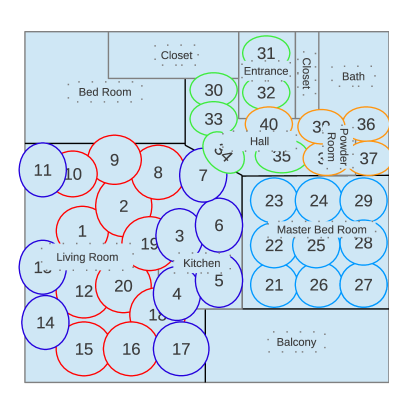
Figure 3: Room layout and sensor locations.

Table 7: Activities in the sensor data set.

ID	Activity	train / test samples
1	Sleeping	81K / 87K
2	Out of Home	66K / 42K
3	Using Computer	64K 46K
4	Relaxing	25K / 65K
5	Eating	6.4K / 6.0K
6	Cooking	5.2K / 4.6K
7	Showering (Bathing)	3.9K / 45.0K
8	No Event	3.4K / 3.5K
9	Using Toilet	2.5K / 2.6K
10	Hygiene (brushing teeth, etc)	1.6K / 1.6K
11	Dishwashing	1.5K / 1.8K
12	Beverage Preparation	1.4K / 1.4K
13	Bath Cleaning / Preparation	0.5K / 0.3K
14	Others	6.5K / 2.1K
Total	-	270K /270K

Two types of features were created: activity-signal features ($40\times 14=560$) and activity-activity features ($14\times 14=196$). Given the aim of sensor number reduction, enforcement of sparseness to individual features can be rather inefficient. Accordingly, we created 40 groups on activity-signal features and each group contained features related to one sensor. Different from the standard independent settings of (1), we considered here a more general form of the criterion function $Q(\mathbf{w})$ by using the negative log-likelihood of a linear-chain conditional random fields model (CRFs, Lafferty et al., 2001).

Specifically, given sample size $N$, let $\mathbf{y}=(y_{1},\cdots,y_{N})^{T}$ be the sequence of action labels with $y_{t}\in\{1,\cdots,14\}$, and let $Z=(\mathbf{z}_{1},\cdots,\mathbf{z}_{N})^{T}$ be the sequence of sensor binary signals with $\mathbf{z}_{t}=(z_{t,1},\cdots,z_{t,40})^{T}\in\{0,1\}^{40}$. Then define the activity-signal features $f_{i,j}(y_{t},\mathbf{z}_{t})=I(y_{t}=j,z_{t,i}=1)$ and the associated sensor coefficients $v_{i,j}$ for $1\leq i\leq 40$, $1\leq j\leq 14$ and $1\leq t\leq N$; define the activity-activity features $g_{i,j}(y_{t},y_{t+1})=I(y_{t}=i,y_{t+1}=j)$ and the associated activity transition coefficients $u_{i,j}$ for $1\leq i,j\leq 14$ and $1\leq t\leq N$. For notation convenience, set $y_{0}=0$. The coefficient vector $\mathbf{v}_{i}=(v_{i,1},\cdots,v_{i,14})^{T}$ then corresponds to the group of sensor $i$ $(1\leq i\leq 40)$. With the targeted goal of sensor selection, we can impose group sparsity on the coefficient $\mathbf{v}=(\mathbf{v}_{1}^{T},\cdots,\mathbf{v}_{40}^{T})^{T}$ since it has a clear grouping structure by construction with 40 groups, while the transition coefficient $\mathbf{u}=(u_{1,1},u_{1,2},\cdots,u_{14,13},u_{14,14})$ is assumed to be dense. Accordingly, the complete coefficient vector is $\mathbf{w}=(\mathbf{v}^{T},\mathbf{u}^{T})^{T}$, and the group selection should focus on the components in $\mathbf{v}$ while allowing elements in $\mathbf{u}$ to be nonezero. Then motivated by Hidden Markov models, the linear-chain CRF objective considers the conditional probability

$$p_{\mathbf{w}}(\mathbf{y}\,|\,Z) ={\frac{1}{q_{\mathbf{w}}(Z)}}\exp\Bigl{\{}\sum_{t=1}^{N}\sum_{i=1}^{40}\sum_{j=1}^{14}v_{i,j}f_{i,j}(y_{t},\mathbf{z}_{t})+\sum_{t=1}^{N}\sum_{i=1}^{14}\sum_{j=1}^{14}u_{i,j}g_{i,j}(y_{t-1},y_{t})\Bigr{\}}$$

$$=:\frac{1}{q_{\mathbf{w}}(Z)}\exp\Bigl{\{}\sum_{t=1}^{N}\bigl{(}\mathbf{v}^{T}\mathbf{f}(y_{t},\mathbf{z}_{t})+\mathbf{u}^{T}\mathbf{g}(y_{t-1},y_{t})\bigr{)}\Bigr{\}}$$

$$=:\frac{1}{q_{\mathbf{w}}(Z)}\tilde{p}_{\mathbf{w}}(\mathbf{y}\,|\,Z),$$ (12)

where $q_{\mathbf{w}}(Z)=\sum_{\tilde{\mathbf{y}}}\tilde{p}_{\mathbf{w}}(\tilde{\mathbf{y}}\,|\,Z)$ is the normalization factor, and $\mathbf{f}$ and $\mathbf{g}$ are vector-valued functions consisting of $(f_{1,1},f_{1,2},\cdots,f_{40,13},f_{40,14})^{T}$ and $(g_{1,1},g_{1,2},\cdots,g_{14,13},g_{14,14})^{T}$, respectively. The resulting negative log-likelihood criterion function is $Q(\mathbf{w})=-\log p_{\mathbf{w}}(\mathbf{y}\,|\,Z)$, which can be shown to be both smooth and convex. Given parameter $\mathbf{w}$, the criterion function’s gradient and the normalization factor (and thus $Q(\mathbf{w})$ itself) can be computed efficiently with a polynomial time of $N$ due to the chain-structured graph and the associated recursive computing scheme (Sutton et al., 2012, Chapter 4.1); the inference for testing data $\tilde{Z}$ can be similarly obtained by maximizing $p_{\mathbf{w}}(\tilde{\mathbf{y}}|\tilde{Z})$ with respective to $\tilde{\mathbf{y}}$. In addition, optimization of the criterion function with respect to $\mathbf{w}$ can be achieved by the generic maximum likelihood estimation (Sutton et al., 2012, Chapter 5.1). With the techniques above, for group/sensor selection purposes, the IGA algorithm can be naturally applied to the criterion function from the negative log-likelihood of (12). In the following experiment, our IGA approach for sensor selection adopted the gradient-based variant as discussed in Section 3.3 and performed the forward-backward selection for groups in $\mathbf{v}$.

We also compared IGA with two other benchmark sensor selection methods: gradient FoBa (FoBa) and Group L1 CRF (GroupLasso). For all three methods, we directly set the numbers for selected sensors (each sensor corresponds to one group of features), as suggested in Zhang (2011a) and Liu et al. (2013). In our specific problem, it is considered informative and convenient to know the classification performance given a specified number of sensors with the practical goal of reducing the number of required sensors (even at a small expense of accuracy). The overall classification error rates on testing samples with varying number of sensors are summarized in Figure 4(a). We discovered the following.

• When the number of sensors was relatively small (5-9), IGA outperformed the other methods. With the sufficient number of sensors, FoBa also performed competitively. We observed big accuracy improvement for FoBa around 10-11 sensors. The lists of selected sensors in Table 8, in together with the corresponding classification results in Figures 4(a), seemed to suggest that the features related to Sensor 28 were important (for a justification, see also discussion below on individual activities). The IGA successfully chose this sensor in early iterations while FoBa used longer iterations.

• IGA required only 7-8 sensors to achieve nearly best performance though FoBa required 11-12 sensors. Therefore, we may reduce 4-5 sensors by using IGA. GroupLasso gradually reduced the classification error with increasing number of sensors, but its classification performance was not ideal in this study when compared to the considered greedy methods.

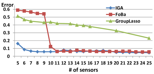
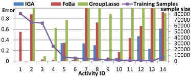
Figure 4: Comparison among FoBa, GroupLasso, and IGA. (a) Classification errors given the number of selected sensors for testing samples (horizontal axis represents number of selected sensors); (b) Activity-wise testing classification errors with 7 sensors (horizontal axis represents activity category ID; solid line is training sample size); (c) Activity-wise testing classification errors with 10 sensors (horizontal axis represents activity category ID; solid line is training sample size).

Table 8: Selected sensors.

Method	7 sensors	10 sensors
IGA	$\{5,8,10,19,28,39,40\}$	$\{7\,\text{sensors}\}\cup\{1,31,35\}$
FoBa	$\{1,5,9,10,19,39,40\}$	$\{7\,\text{sensors}\}\cup\{8,28,35\}$
GroupLasso	$\{1,5,9,10,19,39,40\}$	$\{7\,\text{sensors}\}\cup\{2,36,37\}$

The classification errors for individual activities with 7 sensors and 10 sensors are shown in Figure 4(b) and Figure 4(c), respectively. We can see that for most of the activity categories, with either 7 or 10 sensors, IGA performed generally better than the other two alternatives. Interestingly, recognition errors of FoBa for the activities, Sleeping (Activity ID=1) and Out of Home (Activity ID=2), were quite poor with 7 sensors, but the errors were drastically reduced with 10 sensors. Since both the Sleeping and Out of Home activities have “quiet” movements and generate little sensor signals, they are expected to be difficult to distinguish from each other. Our experiment results in Table 8 showed that FoBa added Sensor 28 at “the number of sensors = 10” and its recognition error dramatically improved. This observation made practical sense as Sensor 28 was located near the bed (shown in Figure 3) and therefore played a key role to distinguish these two activities. This reaffirms our discussion above that Sensor 28 could be an important sensor in practice; with noisy signals from the “quiet” movements, IGA discovered this sensor at earlier steps than FoBa. This experiment showed the promising use of IGA in selecting a small number of sensors while maintaining competitive activity recognition accuracy.

7.   Conclusion

In this paper, we propose a new interactive greedy algorithm designed to exploit known grouping structure for improved estimation and feature group recovery performance. Motivated under a general setting applicable to a broad range of applications, we provide the theoretical and empirical investigations on the proposed algorithm. This study establishes explicit estimation error bounds and group selection consistency results in high-dimensional linear model and logistic regression, and supports that this new algorithm can be a promising and flexible group sparsity learning tool in practice. In the future, it is of interest to conduct further study under the general setting and give explicit performance guarantee for a broader class of GLM models beyond linear and logistic regression. It is also promising to study the performance of our approach under challenging settings including sequential decision making (e.g., Qian and Yang, 2016) and non-smooth objective function (e.g., Gu et al., 2018) problems.

Supplementary Materials

Supplement to “An Interactive Greedy Approach to Group Sparsity in High Dimension”

We provide the proofs of Theorems 4.1 and 4.2 in Supplement A. The proofs for the sparse linear model and the sparse logistic regression are given in Supplement B and Supplement C, respectively. The useful lemmas for intermediate steps of these proofs are relegated to Supplement D. (supplement.pdf)

MATLAB package

The MATLAB package demonstrates the implementation and use of the IGA and GIGA algorithms for both sparse linear model and sparse logistic regression. It is available at https://github.com/weiqian1/IGA.

Supplement to “An Interactive Greedy Approach to Group Sparsity in High Dimension”

In this Supplement, we provide the proofs of Theorems 4.1 and 4.2 in Supplement A, and give the proofs for the sparse linear model and the sparse logistic regressions in Supplement B and Supplement C, respectively. We leave useful lemmas to Supplement D.

Appendix A Proofs of Theorem 4.1 and Theorem 4.2

Theorem 4.1 follows directly from statements of Theorem A.1 and Theorem A.2 in the following.

Theorem A.1.

Suppose Assumption 1 holds and let $\delta$ satisfy $\delta>\frac{4\varphi_{+}(1)}{\lambda\varphi_{-}^{2}(s)}\|\nabla Q(\bar{\mathbf{w}})\|_{G,\infty}^{2}$. Suppose IGA stops at $k$, and the supporting group is $G^{(k)}$ with supporting features as $F^{(k)}=F_{G^{(k)}}$. Then the estimator has the following properties:

$$\|\bar{\mathbf{w}}-\mathbf{w}^{(k)}\| \leqslant\frac{4\sqrt{\varphi_{+}(1)\delta}}{\varphi_{-}(s)}\sqrt{|\bar{\Delta}|}$$ (A.1)

$$Q(\mathbf{w}^{(k)})-Q(\bar{\mathbf{w}}) \leqslant\frac{2\varphi_{+}(1)\delta}{\varphi_{-}(s)}|\bar{\Delta}|$$ (A.2)

$$|\bar{G}\setminus G^{(k)}| \leqslant 2|\bar{\Delta}|$$ (A.3)

$$|G^{(k)}\setminus\bar{G}| \leqslant\frac{16{\varphi}^{2}_{+}(1)|\bar{\Delta}|}{\lambda{\varphi}^{2}_{-}(s)}$$ (A.4)

where $\bar{\Delta}=\{g\in\bar{G}:\|\bar{\mathbf{w}}_{g}\|<\gamma\}$ and $\gamma=\sqrt{\frac{16\varphi_{+}(1)\delta}{\varphi_{-}^{2}(s)}}$.

Proof of Theorem A.1.

After our algorithm terminates, suppose that we have $k$ group selected. From Lemma D.5, we can just assume $Q(\mathbf{w}^{(k)})\geqslant Q(\bar{\mathbf{w}})$ and hence we have:

$$0\geqslant Q(\bar{\mathbf{w}})-Q(\mathbf{w}^{(k)})\geqslant\langle\nabla Q(\mathbf{w}^{(k)}),\bar{\mathbf{w}}-\mathbf{w}^{(k)}\rangle+\frac{\varphi_{-}(s)}{2}\|\bar{\mathbf{w}}-\mathbf{w}^{(k)}\|^{2}$$

After rearranging the above inequality and taking advantage of regrouping, we have

$$\frac{\varphi_{-}(s)}{2}\|\bar{\mathbf{w}}-\mathbf{w}^{(k)}\|^{2}\leqslant-\langle\nabla Q(\mathbf{w}^{(k)}),\bar{\mathbf{w}}-\mathbf{w}^{(k)}\rangle$$

$$=-{\langle\nabla Q(\mathbf{w}^{(k)}),(\bar{\mathbf{w}}-\mathbf{w}^{(k)})_{{\bar{G}{\cup}G^{(k)}}}\rangle}=-{\langle(\nabla Q(\mathbf{w}^{(k)}))_{{\bar{G}{\cup}G^{(k)}}},(\bar{\mathbf{w}}-\mathbf{w}^{(k)})\rangle}$$

$$=-{\langle(\nabla Q(\mathbf{w}^{(k)}))_{{\bar{G}{\setminus}G^{(k)}}},(\bar{\mathbf{w}}-\mathbf{w}^{(k)})\rangle}\qquad(\bar{\mathbf{w}}-\mathbf{w}^{(k)}\textrm{ is supported on }\bar{G}{\setminus}G^{(k)})$$

$$=-{\langle\nabla Q(\mathbf{w}^{(k)}),(\bar{\mathbf{w}}-\mathbf{w}^{(k)})_{{\bar{G}{\setminus}G^{(k)}}}\rangle}\leqslant\|\nabla Q(\mathbf{w}^{(k)})\|_{G,\infty}\|(\bar{\mathbf{w}}-\mathbf{w}^{(k)})_{\bar{G}{\setminus}G^{(k)}}\|_{G,1}$$

$$\leqslant\sqrt{2\varphi_{+}(1)\delta}\sqrt{|\bar{G}{\setminus}G^{(k)}|}\|\bar{\mathbf{w}}-\mathbf{w}^{(k)}\|.\qquad(\textrm{from Lemma \ref{lemma2}})$$

Simplifying the above inequality, we have the following:

$$\|\bar{\mathbf{w}}-\mathbf{w}^{(k)}\| \leqslant\frac{2\sqrt{2\varphi_{+}(1)\delta}}{\varphi_{-}(s)}\sqrt{|\bar{G}{\setminus}G^{(k)}|}.$$ (A.5)

We are interested in estimating errors from certain weak channels of our signals, and mathematically we consider a threshold of coefficients so that we can use the Chebyshev inequality to get new bounds below:

$$\frac{8\varphi_{+}(1)\delta}{\varphi_{-}^{2}(s)}|\bar{G}{{\setminus}}G^{(k)}|\geqslant\|\bar{\mathbf{w}}-\mathbf{w}^{(k)}\|^{2}\geqslant\|(\bar{\mathbf{w}}-\mathbf{w}^{(k)})_{\bar{G}{{\setminus}}G^{(k)}}\|^{2}$$

$$= \,\|\bar{\mathbf{w}}_{\bar{G}{\setminus}G^{(k)}}\|^{2}\qquad(\mathbf{w}^{(k)}\textrm{ is supported outside of }\bar{G}{\setminus}G^{(k)})$$

$$\geqslant \,\gamma^{2}|\{g\in\bar{G}{\setminus}G^{(k)}\ \ |\ \ \|\bar{\mathbf{w}}_{g}\|^{2}\geqslant\gamma^{2}\}|\geqslant\frac{16\varphi_{+}(1)\delta}{\varphi_{-}^{2}(s)}|\{g\in\bar{G}{\setminus}G^{(k)}\ \ |\ \ \|\bar{\mathbf{w}}_{g}\|\geqslant\gamma\}|.$$

We take $\gamma^{2}=\frac{16\varphi_{+}(1)\delta}{\varphi_{-}^{2}(s)}$ in the last inequality and hence we can almost get rid of the coefficients:

$$|\bar{G}{{\setminus}}G^{(k)}|\geqslant 2|\{g\in\bar{G}{\setminus}G^{(k)}\ \ |\ \ \|\bar{\mathbf{w}}_{g}\|\geqslant\gamma\}|=2(|\bar{G}{{\setminus}}G^{(k)}|-|\{g\in\bar{G}{\setminus}G^{(k)}\ \ |\ \ \|\bar{\mathbf{w}}_{g}\|<\gamma\}|).$$

Obviously, this tells a better estimation that we will use often:

$$|\bar{G}{{\setminus}}G^{(k)}|\leqslant 2|\{g\in\bar{G}{\setminus}G^{(k)}\ \ |\ \ \|\bar{\mathbf{w}}_{g}\|<\gamma\}|\leqslant 2|\{g\in\bar{G}\ \ |\ \ \|\bar{\mathbf{w}}_{g}\|<\gamma\}|,$$

which proves the third inequality. Then we can continue our estimation of errors using these new notations. First, we put it in (A.5) we have coefficient error bound

$$\|\bar{\mathbf{w}}-\mathbf{w}^{(k)}\|\leqslant\frac{2\sqrt{2\varphi_{+}(1)\delta}}{\varphi_{-}(s)}\sqrt{|\bar{G}{{\setminus}}G^{(k)}|}\leqslant\frac{4\sqrt{\varphi_{+}(1)\delta}}{\varphi_{-}(s)}\sqrt{|\{g\in\bar{G}{\setminus}G^{(k)}\ \ |\ \ \|\bar{\mathbf{w}}_{g}\|<\gamma\}|}.$$

Second, we bound the loss function error:

$$Q(\bar{\mathbf{w}})-Q(\mathbf{w}^{(k)})\geqslant\langle\nabla Q(\mathbf{w}^{(k)}),\bar{\mathbf{w}}-\mathbf{w}^{(k)}\rangle+\frac{\varphi_{-}(s)}{2}{\|\bar{\mathbf{w}}-\mathbf{w}^{(k)}\|^{2}}$$

$$= \langle\nabla Q(\mathbf{w}^{(k)})_{\bar{G}\cup G^{(k)}},({\bar{\mathbf{w}}-\mathbf{w}^{(k)}})_{\bar{G}\cup G^{(k)}}\rangle+\frac{\varphi_{-}(s)}{2}{\|\bar{\mathbf{w}}-\mathbf{w}^{(k)}\|^{2}}(\bar{\mathbf{w}}-\mathbf{w}^{(k)}$$

$$= \langle\nabla Q(\mathbf{w}^{(k)})_{\bar{G}{{\setminus}}G^{(k)}},({\bar{\mathbf{w}}-\mathbf{w}^{(k)}})_{\bar{G}{{\setminus}}G^{(k)}}\rangle+\frac{\varphi_{-}(s)}{2}{\|\bar{\mathbf{w}}-\mathbf{w}^{(k)}\|^{2}}$$

$$\geqslant -\|\nabla Q(\mathbf{w}^{(k)})\|_{G,\infty}\|\bar{\mathbf{w}}-\mathbf{w}^{(k)}\|_{G,1}+\frac{\varphi_{-}(s)}{2}{\|\bar{\mathbf{w}}-\mathbf{w}^{(k)}\|^{2}}$$

$$\geqslant -\sqrt{2\varphi_{+}(1)\delta|\bar{G}{{\setminus}}G^{(k)}|}\|\bar{\mathbf{w}}-\mathbf{w}^{(k)}\|+\frac{\varphi_{-}(s)}{2}{\|\bar{\mathbf{w}}-\mathbf{w}^{(k)}\|^{2}}\textrm{ (Cauchy-Schwartz inequality)}$$

$$\geqslant -\frac{\varphi_{+}(1)\delta|\bar{G}{{\setminus}}G^{(k)}|}{\varphi_{-}(s)}\geqslant-\frac{2\varphi_{+}(1)\delta}{\varphi_{-}(s)}|\{g\in\bar{G}{\setminus}G^{(k)}\ \ |\ \ \|\bar{\mathbf{w}}_{g}\|<\gamma\}|.$$

Lastly, we bound the error on selection groups. And this is quite easy if we use Lemma D.4 and the first error bound:

$$\frac{\delta^{(k)}}{\varphi_{+}(1)}|G^{(k)}{\setminus}\bar{G}|\leqslant\|(\mathbf{w}^{(k)}-\bar{\mathbf{w}})_{G^{(k)}{\setminus}\bar{G}}\|^{2}\leqslant\frac{16\varphi_{+}(1)\delta}{\varphi_{-}^{2}(s)}|\{g\in\bar{G}{\setminus}G^{(k)}\ \ |\ \ \|\bar{\mathbf{w}}_{g}\|<\gamma\}|.$$

Again, due to our requirement in the algorithm, $\delta^{(k)}\geqslant\lambda\delta$, we then have the bound on the error of group selection as in the lemma. This completes the proof of the lemma. ∎

Theorem A.2.

If we take $\delta>\frac{4\varphi_{+}(1)}{\lambda\varphi_{-}^{2}(s)}\|\nabla Q(\bar{\mathbf{w}})\|_{G,\infty}^{2}$ and require $s$ to satisfy that $s>\bar{k}+(\bar{k}+1)(\sqrt{\kappa(s)}+1)^{2}(\sqrt{2}\kappa(s))^{2}\frac{1}{\lambda}$, where $\bar{k}$ is the number of groups corresponding to $\bar{G}$, then our algorithm will terminate at some $k\leqslant s-\bar{k}$.

Proof of Theorem A.2.

Suppose our algorithm terminates at some number larger than $s-\bar{k}$, then we may just assume the first time $k$ such that $k=s-\bar{k}$. Again, we denote the supporting groups to be $G^{(k)}$ with the optimal point as $\mathbf{w}^{(k)}$. Then we combine $\bar{G}$ and $G^{(k)}$ together to get $G^{\prime}=\bar{G}\cup G^{(k)}$. Denote $\mathbf{w}^{\prime}=\underset{\text{supp}(\mathbf{w})\subset F^{\prime}}{\text{argmin}}Q(\mathbf{w})$, where $F^{\prime}=F_{G^{\prime}}$ . By requirement of $s$, we have $|G^{\prime}|\leqslant s$.

Next, we consider the last step to get $k$ and we have

$$\delta^{(k)}\geqslant \lambda\bigl{(}Q(\mathbf{w}^{(k-1)})-\underset{g\notin G^{(k-1)},\boldsymbol{\alpha}}{\min}Q(\mathbf{w}^{(k-1)}+\mathbf{E}_{g}\boldsymbol{\alpha})\bigr{)}$$

$$\geqslant \frac{\varphi_{-}(s)(Q(\mathbf{w}^{(k-1)})-Q(\mathbf{w}^{\prime}))\lambda^{2}}{\varphi_{+}(1)|G^{\prime}{{\setminus}}G^{(k-1)}|\lambda}\qquad(\textrm{Lemma \ref{forward_process_obj} with }\hat{G}=G^{(k-1)})$$

$$\geqslant \frac{\varphi_{-}(s)(Q(\mathbf{w}^{(k)})-Q(\mathbf{w}^{\prime}))\lambda}{\varphi_{+}(1)|G^{\prime}{{\setminus}}G^{(k-1)}|}\qquad(\textrm{assumption based on}$$

$$\qquad\textrm{algorithm and Lemma }\ref{decrease})$$

$$\geqslant \frac{\varphi_{-}(s)\left(\langle\nabla Q(\mathbf{w}^{\prime}),\mathbf{w}^{(k)}-\mathbf{w}^{\prime}\rangle+\frac{\varphi_{-}(s)}{2}\|\mathbf{w}^{(k)}-\mathbf{w}^{\prime}\|^{2}\right)\lambda}{\varphi_{+}(1)|G^{\prime}{{\setminus}}G^{(k-1)}|}\qquad(\textrm{definition of }\varphi_{-}(s))$$

$$\geqslant \frac{\varphi_{-}^{2}(s)\|\mathbf{w}^{(k)}-\mathbf{w}^{\prime}\|^{2}\lambda}{2\varphi_{+}(1)|G^{\prime}{{\setminus}}G^{(k-1)}|}.\qquad(\mathbf{w}^{\prime}\textrm{ is optimal on }F^{\prime})$$

Now using the result in Lemma D.4 ($\delta^{(k)}\leqslant\frac{\|\mathbf{w}^{(k)}-\bar{\mathbf{w}}\|^{2}\varphi_{+}(1)}{|G^{(k)}{\setminus}\bar{G}|}$) and the fact that $|G^{\prime}{\setminus}\bar{G}|=|G^{(k)}{\setminus}\bar{G}|$, we have the following relation between the two estimations

$$\|\mathbf{w}^{(k)}-\bar{\mathbf{w}}\|^{2}\geqslant\left(\frac{\varphi_{-}(s)}{\sqrt{2}\varphi_{+}(1)}\right)^{2}\left(\frac{\lambda|G^{\prime}{\setminus}\bar{G}|}{|G^{\prime}{{\setminus}}G^{(k-1)}|}\right)\|\mathbf{w}^{(k)}-\mathbf{w}^{\prime}\|^{2}.$$

To simplify our notation we introduce a constant $c=\left(\frac{\varphi_{-}(s)}{\sqrt{2}\varphi_{+}(1)}\right)\left(\sqrt{\frac{\lambda|G^{\prime}{\setminus}\bar{G}|}{|G^{\prime}{{\setminus}}G^{(k-1)}|}}\right).$ As $k=s-\bar{k}$ and $s\geqslant 2\bar{k}+1$, a finer calculation and our requirement for the number $s$ give us the following relation

$$c =\left(\frac{\varphi_{-}(s)}{\sqrt{2}\varphi_{+}(1)}\right)\left(\sqrt{\frac{\lambda|G^{(k)}{\setminus}G^{(k)}\cap\bar{G}|}{|G^{\prime}{{\setminus}}G^{(k)}|+1}}\right)=\left(\frac{\varphi_{-}(s)}{\sqrt{2}\varphi_{+}(1)}\right)\left(\sqrt{\frac{\lambda|G^{(k)}{\setminus}G^{(k)}\cap\bar{G}|}{|\bar{G}{\setminus}G^{(k)}\cap\bar{G}|+1}}\right)$$

$$=\left(\frac{\varphi_{-}(s)}{\sqrt{2}\varphi_{+}(1)}\right)\left(\sqrt{\lambda\frac{|G^{k}|-|G^{(k)}\cap\bar{G}|}{|\bar{G}|-|G^{(k)}\cap\bar{G}|+1}}\right)=\left(\frac{\varphi_{-}(s)}{\sqrt{2}\varphi_{+}(1)}\right)\left(\sqrt{\lambda\frac{k-|G^{(k)}\cap\bar{G}|}{\bar{k}-|G^{(k)}\cap\bar{G}|+1}}\right)$$

$$\geqslant\left(\frac{\varphi_{-}(s)}{\sqrt{2}\varphi_{+}(1)}\right)\left(\sqrt{\lambda\frac{s-\bar{k}}{\bar{k}+1}}\right)\geqslant\sqrt{\kappa(s)}+1.\qquad(\textrm{due to our definition of }s)$$

So we have

$$c\|\mathbf{w}^{(k)}-\mathbf{w}^{\prime}\|\leqslant\|\mathbf{w}^{(k)}-\bar{\mathbf{w}}\|\leqslant\|\mathbf{w}^{(k)}-\mathbf{w}^{\prime}\|+\|\mathbf{w}^{\prime}-\bar{\mathbf{w}}\|,$$ (A.6)

which implies that $(c-1)\|\mathbf{w}^{(k)}-\mathbf{w}^{\prime}\|\leqslant\|\mathbf{w}^{\prime}-\bar{\mathbf{w}}\|$. The following calculation, together with (A.6), shows that $Q(\mathbf{w}^{(k+1)})\leqslant Q(\bar{\mathbf{w}})$:

$$Q(\mathbf{w}^{(k)})-Q(\bar{\mathbf{w}})=Q(\mathbf{w}^{(k)})-Q(\mathbf{w}^{\prime})-(Q(\bar{\mathbf{w}})-Q(\mathbf{w}^{\prime}))$$

$$\leqslant \frac{\varphi_{+}(s)}{2}\|\mathbf{w}^{(k)}-\mathbf{w}^{\prime}\|^{2}-\frac{\varphi_{-}(s)}{2}\|\mathbf{w}^{\prime}-\bar{\mathbf{w}}\|^{2}\leqslant\left(\frac{\varphi_{+}(s)}{2(c-1)^{2}}-\frac{\varphi_{-}(s)}{2}\right)\|\mathbf{w}^{\prime}-\bar{\mathbf{w}}\|^{2}\leqslant 0.$$

However, this contradicts (A.21). So the assumption is incorrect and it completes the proof. ∎

Theorem 4.2 follows directly from statements of Theorem A.3 and Theorem A.4 in the following. We can see that conclusions in Theorems A.3 and A.4 for GIGA are similar to those of Theorems A.1 and A.2 for IGA,

Theorem A.3.

Let $\varepsilon$ in GIGA algorithm satisfy $\varepsilon\geqslant\frac{2\sqrt{2}{\varphi}_{+}(1)\|\nabla Q(\bar{\mathbf{w}})\|_{G,\infty}}{\lambda{\varphi}_{-}(s)}$. Suppose the algorithm stops at $k$, and the supporting group is $G^{(k)}$ with supporting features as $F^{(k)}=F_{G^{(k)}}$. Then the GIGA estimator will satisfy

$$\|\bar{\mathbf{w}}-\mathbf{w}^{(k)}\|^{2} \leqslant\frac{8\varepsilon^{2}\bar{\Delta}}{{\varphi}^{2}_{-}(s)}$$ (A.7)

$$Q(\mathbf{w}^{(k)})-Q(\bar{\mathbf{w}}) \leqslant\frac{{\varepsilon}^{2}\bar{\Delta}}{{\varphi}_{-}(s)}$$ (A.8)

$$|\bar{G}\setminus G^{(k)}| \leq 2\bar{\Delta}$$ (A.9)

$$|G^{(k)}\setminus\bar{G}| \leqslant\frac{16{\varphi}^{2}_{+}(1)\bar{\Delta}}{\lambda^{2}{\varphi}^{2}_{-}(s)}.$$ (A.10)

where $\bar{\Delta}=|\{g\in\bar{G}\setminus G^{(k)}\ \ :\ \ \|\bar{\mathbf{w}}_{g}\|<\gamma\}|$ and $\gamma=\frac{2\sqrt{2}\varepsilon}{{\varphi}_{-}(s)}$.

Proof of Theorem A.3.

By our previous lemmas, if $\varepsilon\geqslant\frac{2\sqrt{2}{\varphi}_{+}(1)\|\nabla Q(\bar{\mathbf{w}})\|_{G,\infty}}{\lambda{\varphi}_{-}(s)}$, we will have

$$0 \geqslant Q(\bar{\mathbf{w}})-Q(\mathbf{w}^{(k)})$$

$$\geqslant\langle\nabla Q(\mathbf{w}^{(k)}),\bar{\mathbf{w}}-\mathbf{w}^{(k)}\rangle+\frac{{\varphi}_{-}(s)\|\bar{\mathbf{w}}-\mathbf{w}^{(k)}\|^{2}}{2}.$$

A simple calculation gives the following relations:

$$\frac{{\varphi}_{-}(s)\|\bar{\mathbf{w}}-\mathbf{w}^{(k)}\|^{2}}{2} \leqslant-\langle\nabla Q(\mathbf{w}^{(k)}),\bar{\mathbf{w}}-\mathbf{w}^{(k)}\rangle$$

$$\leqslant\|\nabla Q(\mathbf{w}^{(k)})\|_{G,\infty}\sqrt{|\bar{G}\setminus G^{(k)}|}\|\bar{\mathbf{w}}-\mathbf{w}^{(k)}\|$$

$$\leqslant\varepsilon\sqrt{|\bar{G}\setminus G^{(k)}|}\|\bar{\mathbf{w}}-\mathbf{w}^{(k)}\|.$$

So we have

$$\|\bar{\mathbf{w}}-\mathbf{w}^{(k)}\|\leqslant\frac{2\varepsilon\sqrt{|\bar{G}\setminus G^{(k)}|}}{{\varphi}_{-}(s)}.$$ (A.11)

Here we point out that when the algorithm terminates, the $\ell_{G,\infty}$ norm is less than $\varepsilon$ not $\lambda\varepsilon$ according to our algorithm. Writing in another form, we have

$$\frac{4\varepsilon^{2}|\bar{G}\setminus G^{(k)}|}{{\varphi}^{2}_{-}(s)} \geqslant\|\bar{\mathbf{w}}-\mathbf{w}^{(k)}\|^{2}$$

$$\geqslant\|(\bar{\mathbf{w}}-\mathbf{w}^{(k)})_{\bar{G}\setminus G^{(k)}}\|^{2}=\|\bar{\mathbf{w}}_{\bar{G}\setminus G^{(k)}}\|^{2}$$

$$\geqslant\gamma^{2}|\{g\in\bar{G}\setminus G^{(k)}\ \ |\ \ \|\bar{\mathbf{w}}_{g}\|\geqslant\gamma\}|.$$

If we let $\gamma^{2}=\frac{8\varepsilon^{2}}{{\varphi}^{2}_{-}(s)}$, we can get a new estimation using the same trick as in IGA:

$$|\bar{G}\setminus G^{(k)}|\leqslant 2|\{g\in\bar{G}\setminus G^{(k)}\ \ |\ \ \|\bar{\mathbf{w}}_{g}\|<\gamma\}|=2\bar{\Delta}.$$

From above, we have

$$Q(\bar{\mathbf{w}})-Q(\mathbf{w}^{(k)})$$

$$\geqslant \langle\nabla Q(\mathbf{w}^{(k)}),\bar{\mathbf{w}}-\mathbf{w}^{(k)}\rangle+\frac{{\varphi}_{-}(s)\|\bar{\mathbf{w}}-\mathbf{w}^{(k)}\|^{2}}{2}$$

$$= \langle\nabla Q(\mathbf{w}^{(k)})_{\bar{G}\setminus G^{(k)}},{\bar{\mathbf{w}}-\mathbf{w}^{(k)}}_{\bar{G}\setminus G^{(k)}}\rangle+\frac{{\varphi}_{-}(s)\|\bar{\mathbf{w}}-\mathbf{w}^{(k)}\|^{2}}{2}$$

$$\geqslant -\|\nabla Q(\mathbf{w}^{(k)})\|_{G,\infty}\|\bar{\mathbf{w}}-\mathbf{w}^{(k)}\|_{G,1}+\frac{{\varphi}_{-}(s)\|\bar{\mathbf{w}}-\mathbf{w}^{(k)}\|^{2}}{2}$$

$$\geqslant -\|\nabla Q(\mathbf{w}^{(k)})\|_{G,\infty}\sqrt{|\bar{G}\setminus G^{(k)}|}\|\bar{\mathbf{w}}-\mathbf{w}^{(k)}\|_{G,2}+\frac{{\varphi}_{-}(s)\|\bar{\mathbf{w}}-\mathbf{w}^{(k)}\|^{2}}{2} (\textrm{Cauchy-Schwartz})$$

$$\geqslant -\varepsilon\sqrt{|\bar{G}\setminus G^{(k)}|}\|\bar{\mathbf{w}}-\mathbf{w}^{(k)}\|+\frac{{\varphi}_{-}(s)\|\bar{\mathbf{w}}-\mathbf{w}^{(k)}\|^{2}}{2}$$

$$\geqslant -\frac{|\bar{G}\setminus G^{(k)}|{\varepsilon}^{2}}{2{\varphi}_{-}(s)}.$$

So we can bound the difference of $Q$ as

$$Q(\mathbf{w}^{(k)})-Q(\bar{\mathbf{w}})\leqslant\frac{|\bar{G}\setminus G^{(k)}|{\varepsilon}^{2}}{2{\varphi}_{-}(s)}\leqslant\frac{\bar{\Delta}{\varepsilon}^{2}}{{\varphi}_{-}(s)}.$$

And the error of parameter estimation (A.11) can be simplified to

$$\|\bar{\mathbf{w}}-\mathbf{w}^{(k)}\|\leqslant\sqrt{\frac{4\varepsilon^{2}|\bar{G}\setminus G^{(k)}|}{{\varphi}^{2}_{-}(s)}}\leqslant\sqrt{\frac{8\varepsilon^{2}\bar{\Delta}}{{\varphi}^{2}_{-}(s)}}.$$

For the group selection, we have the following relation due to Lemma D.8 and (A.22)

$$|G^{(k)}\setminus\bar{G}|\leqslant\frac{2{\varphi}^{2}_{+}(1)\|\bar{\mathbf{w}}-\mathbf{w}^{(k)}\|^{2}}{\lambda^{2}\varepsilon^{2}}\leqslant\frac{16{\varphi}^{2}_{+}(1)\bar{\Delta}}{\lambda^{2}{\varphi}^{2}_{-}(s)}.$$

It completes the proof of Theorem A.3. ∎

We need our algorithm to be terminated in as few steps as possible. If we denote $k$ as the iteration that the algorithm stops, then we will show this $k\leqslant s-\bar{k}$. Here, $s$ is the group sparsity and $\bar{k}$ is the number of supporting groups for the optimal solution.

Theorem A.4.

If $\varepsilon\geqslant\frac{2\sqrt{2}{\varphi}_{+}(1)\|\nabla Q(\bar{\mathbf{w}})\|_{G,\infty}}{\lambda{\varphi}_{-}(s)}$ and we require $s$ to a number such that $s>\bar{k}+(\bar{k}+1)(\sqrt{\kappa(s)}+1)^{2}(2\kappa(s))^{2}\frac{1}{\lambda}$, where $\bar{k}$ is the number of groups corresponding to the global optimal sparse solution. Then our algorithm will terminate at some $k\leqslant s-\bar{k}$.

The proof of Theorem A.4 is similar to that of Theorem A.2 and we thus omit its details.

Appendix B Proofs of Theorems 4.3 and 4.4

Proof of Theorem 4.3.

Consider the following notation for matrix. For a matrix $X$ in $\mathbb{R}^{n\times p}$, $X_{g}$ will be a $\mathbb{R}^{n\times|g|}$ matrix that only keep the columns corresponding to $g$, where $g$ is an index set in $\{1,2,\cdots,p\}$. We denote $\Sigma_{g}=X_{g}^{\top}X_{g}$, For the theorem, we can first show that $\|X_{g}^{\top}\varepsilon\|\leqslant\sqrt{n}\left(\sqrt{|g|}+\sqrt{2\varphi_{+}^{2}(1)\log(\frac{1}{\eta})}\right)$ with probability $1-\eta$. To this end, we have to point out that our columns of $X$ are normalized to $\sqrt{n}$ and hence $X_{g}^{\top}\varepsilon$ will be a $\frac{p}{m}$-variate Gaussian random variable with $n$ on the diagonal of covariance matrix. We further use $\lambda_{i}$ as the eigenvalues of $\Sigma_{g}$ with decreasing order. Using that $tr(\Sigma_{g}^{2})=\lambda^{2}_{1}+\lambda^{2}_{2}+\cdots+\lambda^{2}_{|g|}$ and Proposition 1 of Hsu et al. (2012), we have

$$e^{-t}\geqslant\textbf{Pr}\Bigl{(}||X_{g}^{\top}\varepsilon||^{2}>\sum_{i=1}^{|g|}\lambda_{i}+2\sqrt{\sum_{i=1}^{|g|}\lambda_{i}^{2}t}+2\lambda_{1}t\Bigr{)}$$

$$\geqslant \textbf{Pr}\Bigl{(}||X_{g}^{\top}\varepsilon||^{2}>\sum_{i=1}^{|g|}\lambda_{i}+2\sqrt{2\sum_{i=1}^{|g|}\lambda_{i}\lambda_{1}t}+2\lambda_{1}t\Bigr{)}\geqslant\textbf{Pr}\Bigl{(}||X_{g}^{\top}\varepsilon||\geqslant\sqrt{\sum_{i=1}^{|g|}\lambda_{i}}+\sqrt{2\lambda_{1}t}\Bigr{)}.$$

Substitute $t$ with $\log(\frac{1}{\eta})$ and the facts that $\sum_{i=1}^{|g|}\lambda_{i}=|g|n$ and $\lambda_{1}=\|\Sigma_{g}\|\leqslant n\varphi_{+}(1)$, we have $\|X_{g}^{\top}\varepsilon\|\leqslant\sqrt{n}\left(\sqrt{|g|}+\sqrt{2\varphi_{+}(1)\log(\frac{1}{\eta})}\right)$ with probability $1-\eta$. If we replace $\eta$ as $\frac{\eta}{m}$ for each group $g$ and take the maximal of all group norms, we extend the result to the general case:

$$\underset{g\in G}{\operatorname{max}}\ \|X_{g}^{\top}\varepsilon\|\leqslant\sqrt{n}\left(\sqrt{\underset{g\in G}{\operatorname{max}}|g|}+\sqrt{2\varphi_{+}(1)\log(\frac{m}{\eta})}\right)$$ (A.12)

with probability $1-{\eta}$. Recall our general convex function has a factor of $\frac{1}{2n}$, we have

$$\|\nabla Q(\mathbf{w}^{\ast})\|_{G,\infty}\leqslant\frac{1}{\sqrt{n}}\left(\sqrt{\underset{g\in G}{\operatorname{max}}{|g|}}+\sqrt{2\varphi_{+}(1)\log(\frac{m}{\eta})}\right)$$

with high probability. The major difference between the true solution and optimal solution supported on $S$ with $|S|\leqslant\bar{k}$ is that we need to estimate $X_{g}^{\top}\left(X_{S}(X_{S}^{\top}X_{S})^{-1}X_{S}^{\top}-I_{n}\right)\varepsilon$ instead of $X_{g}^{\top}\varepsilon$ for each group $g$. In fact, we are considering $I_{n}-X_{S}(X_{S}^{\top}X_{S})^{-1}X_{S}^{\top}$ since the noise itself makes this negative sign not important. Note, we can decompose $I_{n}-X_{S}(X_{S}^{\top}X_{S})^{-1}X_{S}^{\top}=P_{g}P_{g}^{\top}$, where $P_{g}$ has dimension $n\times(n-|F_{S}|)$ and $P_{g}^{\top}P_{g}=I_{n-|F_{S}|}$, due to the property of the projection matrix $X_{S}(X_{S}^{\top}X_{S})^{-1}X_{S}^{\top}$. That is, we transform our question into estimating $X_{g}^{\top}P_{g}\varepsilon^{\prime}$, where $\varepsilon^{\prime}$ is a vector of i.i.d. $\mathcal{N}(0,1)$ random variables of dimension $n-|F_{S}|$. We denote the largest eigenvalue of $X_{g}^{\top}P_{g}P_{g}^{\top}X_{g}$ as $\lambda^{\prime}$ and it’s easy to observe that $\lambda^{\prime}\leqslant\lambda$. Also the trace of $X_{g}^{\top}P_{g}P_{g}^{\top}X_{g}$ is no big than the trace of $X_{g}^{\top}X_{g}$, so we easily extend the above result to the optimal value and we have $\|\nabla Q(\bar{\mathbf{w}})\|_{G,\infty}\leqslant\frac{1}{\sqrt{n}}\left(\sqrt{\underset{g\in G}{\operatorname{max}}{|g|}}+\sqrt{2\varphi_{+}(1)\log(m)}\right)$ with high probability. The second statement follows by arguments similar to that of (A.12). This completes the proof. ∎

Proof of Theorem 4.4.

In light of Theorem 4.1, we intend to show $\bar{\Delta}\leq\Delta_{\text{IGA}}$ when two constants “$\Omega$’s” are appropriately chosen. It suffices to show that if $\|\bar{\mathbf{w}}_{g}\|<\Omega(\|\nabla Q(\bar{\mathbf{w}})\|_{G,\infty})=\Omega\left(\sqrt{{p\over mn}+{\log(m)\over n}}\right)$ holds, then $\|\mathbf{w}^{*}_{g}\|\leq\Omega\left(\sqrt{{p\over mn}+{\log(m)\over n}}\right)$; Indeed, by the second statement of Theorem 4.3, $\|\mathbf{w}_{g}^{*}\|\leqslant\|\bar{\mathbf{w}}_{g}\|+\|(\bar{\mathbf{w}}-\mathbf{w}^{*})_{g}\|\leq\Omega\left(\sqrt{\frac{{p\over m}+\log m}{n}}\right)$. Then, combining the second statement in Theorem 4.1, $\bar{\Delta}\leq\Delta_{\text{IGA}}$ and the fact that $\lVert\mathbf{w}^{*}-\bar{\mathbf{w}}\rVert=O_{p}(k_{*}/n)$, we obtain the first claim. Combining the last claim in Theorem 4.1 with $\bar{\Delta}\leq\Delta_{\text{IGA}}$ implies the second claim. The proof of Theorem 4.4 is complete. ∎

Appendix C Proofs of Theorems 4.5 and 4.6

Proof of Theorem 4.5.

Define $\tilde{\mathbf{y}}=(\tilde{y}_{1},\cdots,\tilde{y}_{n})^{T}$, where $\tilde{y}_{i}=(y_{i}+1)/2$. We then have $\nabla Q(\mathbf{w})=X^{T}(\mathbf{p}(\mathbf{w})-\tilde{\mathbf{y}})$, where $\mathbf{p}(\mathbf{w})=(p_{1}(\mathbf{w}),\cdots,p_{n}(\mathbf{w}))^{T}$. Since $\mathrm{E}(\tilde{\mathbf{y}}|X)=\mathbf{p}(\mathbf{w})$ and $\tilde{y}_{i}$’s are bounded, the upper-bound statement on gradient group norm $\|\nabla Q(\mathbf{w}^{\ast})\|_{G,\infty}$ follows from similar arugments as (A.12). Next, we intend to show the upper bound for $\lVert\bar{\mathbf{w}}-\mathbf{w}^{*}\rVert_{G,\infty}$. Given $r>0$, define $r$-radius ball in $\ell_{G,\infty}$ norm as $B(r)=\{\Delta\in\mathbb{R}^{p}:\lVert\Delta_{\bar{G}}\rVert_{\bar{G},\infty}\leq r,\,\Delta_{G\backslash\bar{G}}=\mathbf{0}\}$. Define function $H:B(r)\subset\mathbb{R}^{p}\rightarrow\mathbb{R}^{p}$ to be $H_{\bar{G}}(\Delta)=(X_{\bar{G}}^{T}W^{*}X_{\bar{G}})^{-1}X_{\bar{G}}^{T}(\tilde{\mathbf{y}}-\mathbf{p}(w^{*}+\Delta))+\Delta_{\bar{G}}$, and $H_{G\backslash\bar{G}}(\Delta)=\mathbf{0}$. First, note that for any small $\eta>0$, there is some $r_{n}=\Omega(\sqrt{\frac{q+\log m}{n}})$ such that $\mathcal{A}_{n}:=\{H(B(r_{n}))\subset B(r_{n})\}$ holds with probabiity greater than $1-\eta$ for large enough $n$. Indeed, Suppose that $\Delta\in B(r_{n})$ and the event $\mathcal{B}_{n}:=\{\lVert X_{\bar{G}}^{T}W^{*}X_{\bar{G}})^{-1}X_{\bar{G}}^{T}(\mathbf{p}(\mathbf{w}^{*})-\tilde{\mathbf{y}})\rVert_{\bar{G},\infty}\leq r_{n}/2\}$ holds. By Taylor expansion, there is $\tilde{\Delta}\in B(r_{n})$ with same signs of $\Delta$ such that

$$X_{\bar{G}}^{T}\mathbf{p}(\mathbf{w}^{*}+\Delta) =X_{\bar{G}}^{T}\mathbf{p}(\mathbf{w}^{*})+X_{\bar{G}}^{T}W^{*}X_{\bar{G}}\Delta_{\bar{G}}+X_{\bar{G}}^{T}\bigl{(}W(\mathbf{w}^{*}+\tilde{\Delta})-W^{*}\bigr{)}X_{\bar{G}}\Delta_{\bar{G}}$$

$$=:X_{\bar{G}}^{T}\mathbf{p}(\mathbf{w}^{*})+X_{\bar{G}}^{T}W^{*}X_{\bar{G}}\Delta_{\bar{G}}+R_{\bar{G}}(\tilde{\Delta}),$$ (A.13)

where $R(\tilde{\Delta})=X^{T}\bigl{(}W(\mathbf{w}^{*}+\tilde{\Delta})-W^{*}\bigr{)}X_{\bar{G}}\Delta_{\bar{G}}$. Consequently, by the mean value theorem and boundedness of covariate domain and $U_{1}$, there is a positive constant $C_{11}$ such that

$$\lVert R(\tilde{\Delta})\rVert_{G,\infty}\leq\max_{g\in G}\sum_{i=1}^{n}\lVert\mathbf{x}_{ig}\rVert\tilde{\Delta}^{T}\mathbf{x}_{i}^{T}\mathbf{x}_{i}\Delta\leq nC_{11}\bar{k}^{1/2}\lVert\Delta\rVert_{G,\infty}^{2}\leq nC_{11}\bar{k}^{1/2}r_{n}^{2}.$$ (A.14)

The two displays above together with boundedness of $U_{2}$ imply that

$$H_{\bar{G}}(\Delta)=(X_{\bar{G}}^{T}W^{*}X_{\bar{G}})^{-1}\big{(}X_{\bar{G}}^{T}(\mathbf{y}-\mathbf{p}(\mathbf{w}^{*}))-R_{\bar{G}}(\tilde{\Delta})\bigr{)},$$

$$\lVert H_{\bar{G}}(\Delta)\rVert_{\bar{G},\infty}\leq r_{n}/2+\lVert(X_{\bar{G}}^{T}W^{*}X_{\bar{G}})^{-1}R(\tilde{\Delta})\rVert_{\bar{G},\infty}\leq r_{n}/2+C_{11}\bar{k}r_{n}^{2}.$$

In addition, by Hsu et al. (2012), we can obtain that $P(\mathcal{B}_{n})>1-\eta$ with some $r_{n}=\Omega(\sqrt{\frac{q+\log m}{n}})$. In together with previous display and our choice of $r_{n}$, we obtain that $P(\mathcal{A}_{n})>1-\eta$ for large enough $n$.

Next, suppose $\mathcal{A}_{n}$ holds. By Brouwer’s fixed-point theorem, there exists a point $\hat{\Delta}\in B(r_{n})$ such that $H(\hat{\Delta})=\hat{\Delta}$, which implies that $X_{\bar{G}}^{T}(\tilde{\mathbf{y}}-\mathbf{p}(\mathbf{w}^{*}+\hat{\Delta}))=0$ and $\hat{\Delta}_{G\backslash\bar{G}}=\mathbf{0}$. By uniqueness of $\bar{\mathbf{w}}$, we have $\Delta=\bar{\mathbf{w}}-\mathbf{w}^{*}$, and therefore, $\lVert\bar{\mathbf{w}}-\mathbf{w}^{*}\rVert_{G,\infty}=\lVert\hat{\Delta}\rVert_{G,\infty}\leq r_{n}$.

It remains to show the upper bound statement on $\|\nabla Q(\bar{\mathbf{w}})\|_{G,\infty}$. By arguments similar to that of (A.13) and setting $\Delta=\hat{\Delta}$, we have

$$\nabla Q(\bar{\mathbf{w}})=\nabla Q(\mathbf{w}^{*})+\frac{1}{n}X^{T}W^{*}X_{\bar{G}}\hat{\Delta}_{\bar{G}}+\frac{1}{n}R(\tilde{\Delta}).$$

Since $\nabla_{\bar{G}}Q(\bar{\mathbf{w}})=\mathbf{0}$, previous display implies that

$$\hat{\Delta}_{\bar{G}} =(\frac{1}{n}X_{\bar{G}}^{T}W^{*}X_{\bar{G}})^{-1}\bigl{(}-\frac{1}{n}X_{\bar{G}}^{T}(\mathbf{p}(\mathbf{w}^{*})-\tilde{\mathbf{y}})-\frac{1}{n}R_{\bar{G}}(\tilde{\Delta})\bigr{)},$$

$$\nabla_{G\backslash\bar{G}}Q(\bar{\mathbf{w}}) =\nabla_{G\backslash\bar{G}}Q(\mathbf{w}^{*})-\frac{1}{n}\Theta X_{\bar{G}}^{T}(\mathbf{p}(\mathbf{w}^{*})-\tilde{\mathbf{y}})-\frac{1}{n}\Theta R_{\bar{G}}(\tilde{\Delta})+\frac{1}{n}R_{G\backslash\bar{G}}(\tilde{\Delta}),$$ (A.15)

where $\Theta=\frac{1}{n}X_{G\backslash\bar{G}}^{T}W^{*}X_{\bar{G}}(\frac{1}{n}X_{\bar{G}}^{T}W^{*}X_{\bar{G}})^{-1}$. Since $U_{2}$ and $U_{3}$ are bounded, following arguments like (A.12), the second term in (A.15) is upper bounded by $O_{p}(\sqrt{\frac{q+\log m}{n}})$ in $l_{G,\infty}$ norm as the first term; following arguments like (A.14), the third and fourth terms are $O_{p}(\bar{k}r_{n}^{2})$. Therefore, $\lVert\nabla Q(\bar{\mathbf{w}})\rVert_{G,\infty}\leq O_{p}(\sqrt{\frac{q+\log m}{n}})$. We complete the proof of Theorem 4.5. ∎

With Theorem 4.5, Theorem 4.6 can be proved by similar procedures as that of Theorem 4.4.

Appendix D Lemmas and Proofs

In the following, Lemma D.1 connects Assumption 1 to a natural random design scenario. Lemmas D.2–D.6 are useful intermediate results for our analysis of the IGA algorithm, and Lemmas D.7–D.10 are useful for the GIGA algorithm.

Lemma D.1.

Let $Q(\mathbf{w})={1\over n}\sum_{i=1}^{n}f_{i}(\mathbf{x}_{i}^{\top}\mathbf{w})$. All data points $\mathbf{x}_{i}$’s follow from i.i.d. isotropic sub-Gaussian distribution with enough samples $n\geq\Omega(k_{\bar{k}}+\bar{k}\log m)$. Let $L:=\sup\limits_{z\in\mathcal{Z}}(\nabla^{2}f_{i}(z))$ and $l=\inf\limits_{z\in\mathcal{Z}}(\nabla^{2}f_{i}(z))$ where $\mathcal{Z}:=\{\mathbf{x}_{i}^{\top}\mathbf{w}:\leavevmode\nobreak\ \mathbf{w}\in\mathcal{D},\forall i=1,2,\cdots\}$. The condition number $\tau$ is defined as $\tau:={L\over l}$. If the condition number $\tau$ is bounded, then with high probability there exists an $s$ satisfying Assumption 1.

Proof to Lemma D.1.

Let the upper bound of the maximal eigenvalue and the lower bound of the minimal eigenvalue of $\nabla^{2}f(z)$ be $L$ and $l$ respectively. The condition number $\tau$ is defined as $\tau={L/l}$. With slight abuse of notation, let $g$ be an index set in $\{1,\cdots,p\}$. By (6) and the convexity of $f_{i}(\cdot)$, we have

$$n\rho_{+}(g)= \lambda_{\max}\left(\sum_{i=1}^{n}(\mathbf{x}_{i})_{g}(\mathbf{x}_{i})_{g}^{\top}\nabla^{2}f_{i}(\mathbf{x}_{i}^{\top}\mathbf{w})\right)$$

$$\leq \max_{z,i}\nabla^{2}f_{i}(z)\lambda_{\max}\left(\sum_{i=1}^{n}(\mathbf{x}_{i})_{g}(\mathbf{x}_{i})_{g}^{\top}\right)$$

$$\leq L\lambda_{\max}\left(\sum_{i=1}^{n}(\mathbf{x}_{i})_{g}(\mathbf{x}_{i})_{g}^{\top}\right).$$ (A.16)

Similarly, for $\rho_{-}(g)$, we have

$$n\rho_{-}(g)\geq l\lambda_{\min}\left(\sum_{i=1}^{n}(\mathbf{x}_{i})_{g}(\mathbf{x}_{i})_{g}^{\top}\right).$$

Let $T_{s}$ be a super set: $T_{s}=\{F_{S}\leavevmode\nobreak\ |\leavevmode\nobreak\ |S|\leq s,S\subset G\}$ and $k_{s}:=\max\limits_{g\in T_{s}}|g|$. From the random matrix theory (Vershynin, 2010, Theorem 5.39), for any $g\in T_{s}$ we have

$$\sqrt{\lambda_{\max}\left(\sum_{i=1}^{n}(\mathbf{x}_{i})_{g}(\mathbf{x}_{i})_{g}^{\top}\right)}\geq\sqrt{n}+\Omega(\sqrt{|g|})+\Omega(t)$$ (A.17)

holds with probability at most $\exp\{-t^{2}\}$. Then we use the union bound to provide an upper probability bound for $\varphi_{+}(s)$

$$\mathbf{Pr}\left(\sqrt{n\varphi_{+}(s)/L}\geq\sqrt{n}+\Omega(\sqrt{k_{s}})+\Omega(t)\right)$$

$$\leq \sum_{g\in T_{s}}\mathbf{Pr}\left(\sqrt{n\varphi_{+}(s)/L}\geq\sqrt{n}+\Omega(\sqrt{k_{s}})+\Omega(t)\right)$$

$$\leq \sum_{g\in T_{s}}\mathbf{Pr}\left(\sqrt{n\varphi_{+}(s)/L}\geq\sqrt{n}+\Omega(\sqrt{|g|})+\Omega(t)\right)$$

$$\leq \left(\begin{matrix}m\\ s\end{matrix}\right)\exp\{-t^{2}\}\quad (\text{from \eqref{eq:proof_cond_1} and \eqref{eq:proof_cond_2}})$$

$$\leq \exp\{s\log(m)-t^{2}\}.$$

Taking $t=\Omega(\sqrt{s\log m})$, it follows

$$\mathbf{Pr}\left(\sqrt{n\varphi_{+}(s)/L}\geq\sqrt{n}+\Omega(\sqrt{k_{s}}+\sqrt{s\log m})\right)\leq\exp\{-\Omega(s\log m)\}.$$ (A.18)

Similarly, we have

$$\mathbf{Pr}\left(\sqrt{n\varphi_{-}(s)/l}\geq\sqrt{n}-\Omega(\sqrt{k_{s}}+\sqrt{s\log m})\right)\leq\exp\{-\Omega(s\log m)\}.$$ (A.19)

Now we are ready to bound $\tau(s)$. We can choose the value of $n$ large enough such that $\sqrt{n}$ is greater than $3\Omega(\sqrt{k_{s}}+\sqrt{s\log m})$, which indicates

$$\mathbf{Pr}\left(\sqrt{n\varphi_{+}(s)/L}\leq{{4\over 3}\sqrt{n}}\right)\geq 1-\exp\{-\Omega(s\log m)\}$$

and

$$\mathbf{Pr}\left(\sqrt{n\varphi_{-}(s)/l}\geq{{2\over 3}\sqrt{n}}\right)\geq 1-\exp\{-\Omega(s\log m)\}$$

It follows that

$$\mathbf{Pr}(\kappa(s)\leq{2}\tau)=\mathbf{Pr}\left(\frac{\sqrt{n\varphi_{+}(s)/L}}{\sqrt{n\varphi_{-}(s)/l}}\leq{\sqrt{2}}\right)\geq 1-2\exp\{-\Omega(s\log m)\}.$$ (A.20)

Since $\tau$ is bounded, there exists an $s=\Omega(\bar{k})$ satisfying Assumption 1. The required number of samples is $n\geq\Omega(k_{s}+s\log m)=\Omega(k_{\Omega(\bar{k})}+\Omega(\bar{k})\log m)=\Omega(k_{\bar{k}}+\bar{k}\log m)$. It completes the proof. ∎

For analysis of the IGA algorithm, we transform the difference of criteria functions into the norms of the partial derivatives of $Q$.

Lemma D.2.

For any group $g\in G$ and $\mathbf{w}\in\mathcal{D}$, if

$$Q(\mathbf{w})-\underset{\boldsymbol{\alpha}\in\mathbb{R}^{|g|}}{\operatorname{min}}Q(\mathbf{w}+\mathbf{E}_{g}\boldsymbol{\alpha})\geqslant\lambda\delta,$$

then

$$\|\nabla_{g}Q(\mathbf{w})\|\geqslant\sqrt{2\varphi_{-}(1)\lambda\delta}.$$

Proof of Lemma D.2.

Note that we specify the dimension of $\boldsymbol{\alpha}$ explicitly here, but it is quite trivial to find the correct dimension and hence we will ignore the specific dimension from now on for the simplicity of calculation. Taking the parameter $\lambda$ into considerations, we have

$$-\lambda\delta \geqslant\underset{\boldsymbol{\alpha}}{\operatorname{min}}\ Q(\mathbf{w}+\mathbf{E}_{g}\boldsymbol{\alpha})-Q(\mathbf{w})$$

$$\geqslant\underset{\boldsymbol{\alpha}}{\operatorname{min}}\ \langle\nabla Q(\mathbf{w}),\mathbf{E}_{g}\boldsymbol{\alpha}\rangle+\frac{\varphi_{-}(1)}{2}\|\mathbf{E}_{g}\boldsymbol{\alpha}\|^{2} (\textrm{from the definition of $\varphi_{-}(1)$})$$

$$=\underset{\boldsymbol{\alpha}}{\operatorname{min}}\ \langle\nabla_{g}Q(\mathbf{w}),\boldsymbol{\alpha}\rangle+\frac{\varphi_{-}(1)}{2}\|\boldsymbol{\alpha}\|^{2}$$

$$=-\frac{\|\nabla_{g}Q(\mathbf{w})\|^{2}}{2\varphi_{-}(1)}.$$

Hence we have $\|\nabla_{g}Q(\mathbf{w})\|\geqslant\sqrt{2\varphi_{-}(1)\lambda\delta}$ and this completes the proof of the lemma. ∎

Similarly, we can have a conclusion in the other direction.

Lemma D.3.

For any $\mathbf{w}\in\mathcal{D}$, if $\displaystyle{{Q(\mathbf{w})}-\underset{g\in G,\boldsymbol{\alpha}}{\operatorname{min}}Q(\mathbf{w}+\mathbf{E}_{g}\boldsymbol{\alpha})}\leqslant\delta$, then

$$\|\nabla Q(\mathbf{w})\|_{G,\infty}\leqslant\sqrt{2\varphi_{+}(1)\delta}.$$

Proof of Lemma D.3.

Note that

$$\delta \geqslant Q(\mathbf{w})-\underset{g\in G,\boldsymbol{\alpha}}{\operatorname{min}}Q(\mathbf{w}+\mathbf{E}_{g}\boldsymbol{\alpha})$$

$$=\underset{g\in G,\boldsymbol{\alpha}}{\operatorname{max}}-\left(Q(\mathbf{w}+\mathbf{E}_{g}\boldsymbol{\alpha})-Q(\mathbf{w})\right)$$

$$\geqslant\underset{g\in G,\boldsymbol{\alpha}}{\operatorname{max}}-\langle\nabla Q(\mathbf{w}),\mathbf{E}_{g}\boldsymbol{\alpha}\rangle-\frac{\varphi_{+}(1)}{2}\|\mathbf{E}_{g}\boldsymbol{\alpha}\|^{2} (\textrm{from the definition of $\varphi_{+}(1)$})$$

$$=\underset{g\in G,\boldsymbol{\alpha}}{\operatorname{max}}-\langle\nabla_{g}Q(\mathbf{w}),\boldsymbol{\alpha}\rangle-\frac{\varphi_{+}(1)}{2}\|\boldsymbol{\alpha}\|^{2}$$

$$=\underset{g\in G}{\operatorname{max}}\ \frac{\|\nabla_{g}Q(\mathbf{w})\|^{2}}{2\varphi_{+}(1)}$$

$$=\frac{\|\nabla Q(\mathbf{w})\|^{2}_{G,\infty}}{2\varphi_{+}(1)}.$$

Taking square roots on both sides, we can find the relation in the lemma. And it completes the proof. ∎

Due to the stop condition in IGA algorithm, we have the following relations between the group selections and parameter estimations.

Lemma D.4.

At the end of each backward step and hence when our algorithm stops, we have the following connections of our selected parameters and groups:

$$\|\mathbf{w}^{(k)}_{G^{(k)}{\setminus}\bar{G}}\|^{2}=\|(\mathbf{w}^{(k)}-\bar{\mathbf{w}})_{G^{(k)}{\setminus}\bar{G}}\|^{2}\geqslant\frac{\delta^{(k)}}{\varphi_{+}(1)}|G^{(k)}{\setminus}\bar{G}|\geqslant\frac{\lambda\delta}{\varphi_{+}(1)}|G^{(k)}{\setminus}\bar{G}|.$$

Proof of Lemma D.4.

Let’s consider all candidates of removal groups in the backward step, and we have

$$|G^{(k)}{\setminus}\bar{G}|\underset{g\in G^{(k)}{\setminus}\bar{G}}{\operatorname{min}}Q(\mathbf{w}^{(k)}-\mathbf{w}^{(k)}_{g})$$

$$\leqslant \underset{g\in G^{(k)}{\setminus}\bar{G}}{\sum}Q(\mathbf{w}^{(k)}-\mathbf{w}^{(k)}_{g})$$

$$\leqslant \underset{g\in G^{(k)}{\setminus}\bar{G}}{\sum}\left(Q(\mathbf{w}^{(k)})-\langle\nabla Q(\mathbf{w}^{(k)}),\mathbf{w}^{(k)}_{g}\rangle\right)+\underset{g\in G^{(k)}{\setminus}\bar{G}}{\sum}\frac{\varphi_{+}(1)}{2}\|\mathbf{w}^{(k)}_{g}\|^{2}$$

$$= |G^{(k)}{\setminus}\bar{G}|Q(\mathbf{w}^{(k)})+\frac{\varphi_{+}(1)}{2}\|\mathbf{w}^{(k)}_{{G^{(k)}{\setminus}\bar{G}}}\|^{2}. (\mathbf{w}^{(k)}\textrm{ is the optimal on }G^{(k)})$$

Hence, we have

$$|G^{(k)}{\setminus}\bar{G}|\underset{g\in G^{(k)}}{\operatorname{min}}Q\left(\mathbf{w}^{(k)}-\mathbf{w}^{(k)}_{g})-Q(\mathbf{w}^{(k)}\right)\leqslant\frac{\varphi_{+}(1)}{2}\|\mathbf{w}^{(k)}_{G^{(k)}{\setminus}\bar{G}}\|^{2}.$$

Recall the fact that, in the backward algorithm, we will stop at the point where the left hand side is no less than $\frac{\delta^{(k)}}{2}$. Hence, we have $\|\mathbf{w}^{(k)}_{G^{(k)}{\setminus}\bar{G}}\|^{2}\geqslant\frac{|G^{(k)}{\setminus}\bar{G}|\delta^{(k)}}{\varphi_{+}(1)}$. The first two equalities in the lemma are trivial observations, and the last inequality is due to the requirement that $\delta^{(k)}>\lambda\delta$ in our Algorithm 1. It completes the proof of the lemma. ∎

The above Lemma D.4 will help us in transforming the sparsity condition into estimating the errors of the parameters. Moreover, using this idea, we can just concentrate on the case where our selection of groups is no better than “ideal” sparse solution we assumed as shown below.

Lemma D.5.

For any integer $s$ larger than $|G^{(k)}{\setminus}\bar{G}|$, and if

$$\delta>\frac{4\varphi_{+}(1)}{\lambda\varphi_{-}^{2}(s)}\|\nabla Q(\bar{\mathbf{w}})\|_{G,\infty}^{2},$$

then at the end of each backward step $k$, we have

$$Q(\mathbf{w}^{(k)})\geqslant Q(\bar{\mathbf{w}}).$$ (A.21)

Proof of Lemma D.5.

Considering the difference of the two values, we have

$$Q(\mathbf{w}^{(k)})-Q(\bar{\mathbf{w}})$$

$$\geqslant \langle\nabla Q(\bar{\mathbf{w}}),\mathbf{w}^{(k)}-\bar{\mathbf{w}}\rangle+\frac{\varphi_{-}(s)}{2}\|\mathbf{w}^{(k)}-\bar{\mathbf{w}}\|^{2}$$

$$= \langle\nabla Q(\bar{\mathbf{w}}),{(\mathbf{w}^{(k)}-\bar{\mathbf{w}})}_{{G^{(k)}\setminus\bar{G}}}\rangle+\frac{\varphi_{-}(s)}{2}\|\mathbf{w}^{(k)}-\bar{\mathbf{w}}\|^{2}$$

$$\geqslant -\|\nabla Q(\bar{\mathbf{w}})\|_{G,\infty}\|\mathbf{w}^{(k)}-\bar{\mathbf{w}}\|_{G,1}+\frac{\varphi_{-}(s)}{2}\|\mathbf{w}^{(k)}-\bar{\mathbf{w}}\|^{2}$$

$$\geqslant -\|\nabla Q(\bar{\mathbf{w}})\|_{G,\infty}\|\mathbf{w}^{(k)}-\bar{\mathbf{w}}\|\sqrt{|G^{(k)}{\setminus}\bar{G}|}+\frac{\varphi_{-}(s)}{2}\|\mathbf{w}^{(k)}-\bar{\mathbf{w}}\|^{2} (\textrm{Cauchy-Schwartz})$$

$$\geqslant -\|\nabla Q(\bar{\mathbf{w}})\|_{G,\infty}\|\mathbf{w}^{(k)}-\bar{\mathbf{w}}\|^{2}\sqrt{\frac{\varphi_{+}(1)}{\delta^{(k)}}}+\frac{\varphi_{-}(s)}{2}\|\mathbf{w}^{(k)}-\bar{\mathbf{w}}\|^{2}. (\textrm{Lemma\leavevmode\nobreak\ \ref{backward}})$$

Finally, from our choice of $\delta$ and the fact that $\delta^{(k)}>\lambda\delta$, we can then conclude that the last line is bigger than $0$. Hence we will have general assumption $Q(\mathbf{w}^{(k)})\geqslant Q(\bar{\mathbf{w}})$ if $\delta>\frac{4\varphi_{+}(1)}{\varphi_{-}^{2}(s)}\|\nabla Q(\bar{\mathbf{w}})\|_{G,\infty}^{2}$. This completes the proof of the lemma. ∎

One key part of the proof idea is to compare the difference of the convex function at different optimal values supported on different groups with some other quantities. We have the following.

Lemma D.6.

Suppose that $\hat{G}$ is a subset of the super set $G$ and we set $\hat{\mathbf{w}}=\underset{\operatorname{supp}(\mathbf{w})\subset F_{\hat{G}}}{\operatorname{argmin}}Q(\mathbf{w}).$ For any $\mathbf{w}^{\prime}$ with supporting groups $G^{\prime}$ and corresponding features $F^{\prime}=F_{G^{\prime}}$, if

$$g\in\{\bar{g}\in G^{\prime}{{\setminus}}\hat{G}\ \ |\ \ Q(\hat{\mathbf{w}})-\underset{\boldsymbol{\alpha}}{\operatorname{min}}\ Q(\hat{\mathbf{w}}+\mathbf{E}_{\bar{g}}\boldsymbol{\alpha})\geqslant\lambda(Q(\hat{\mathbf{w}})-\underset{\tilde{g}\in G^{\prime}{{\setminus}}\hat{G},\boldsymbol{\alpha}}{\operatorname{min}}Q(\hat{\mathbf{w}}+\mathbf{E}_{\tilde{g}}\boldsymbol{\alpha}))\},$$

then we have

$$Q(\hat{\mathbf{w}})-Q(\mathbf{w}^{\prime})\leqslant\frac{\varphi_{+}(1)|G^{\prime}{\setminus}\hat{G}|(Q(\hat{\mathbf{w}})-\underset{\boldsymbol{\alpha}}{\operatorname{min}}Q(\hat{\mathbf{w}}+\mathbf{E}_{g}\boldsymbol{\alpha}))}{\lambda\varphi_{-}(s)}.$$

Proof of Lemma D.6.

We are comparing the differences of the convex function and its value along the following special directions.

$$|G^{\prime}{{\setminus}}\hat{G}|\underset{g\in G^{\prime}{{\setminus}}\hat{G},\eta}{\operatorname{min}}Q({\hat{\mathbf{w}}}+\eta({\mathbf{w}}_{g}^{\prime}-{\hat{\mathbf{w}}}_{g}))$$

$$\leqslant \underset{g\in G^{\prime}{{\setminus}}\hat{G}}{\sum}Q({\hat{\mathbf{w}}}+\eta({\mathbf{w}}_{g}^{\prime}-{\hat{\mathbf{w}}}_{g})) (\textrm{any }\eta)$$

$$\leqslant \underset{g\in G^{\prime}{{\setminus}}\hat{G}}{\sum}\left(Q({\hat{\mathbf{w}}})+\langle\eta({\mathbf{w}}_{g}^{\prime}-{\hat{\mathbf{w}}}_{g}),\nabla Q({\hat{\mathbf{w}}})\rangle+\frac{\varphi_{+}(1)}{2}\|\eta({\mathbf{w}}_{g}^{\prime}-{\hat{\mathbf{w}}}_{g})\|^{2}\right) (\textrm{definition of }\varphi_{+}(1))$$

$$\leqslant |G^{\prime}{{\setminus}}\hat{G}|Q(\hat{\mathbf{w}})+\langle{\eta}(\mathbf{w}^{\prime}-\hat{\mathbf{w}})_{G^{\prime}{\setminus}\hat{G}},\nabla Q({\hat{\mathbf{w}}})\rangle+\frac{\varphi_{+}(1)}{2}\|\eta(\mathbf{w}^{\prime}-\hat{\mathbf{w}})\|^{2} (\textrm{non-intersection property})$$

$$= |G^{\prime}{{\setminus}}\hat{G}|Q(\hat{\mathbf{w}})+\langle{\eta}(\mathbf{w}^{\prime}-\hat{\mathbf{w}}),(\nabla Q(\hat{\mathbf{w}}))_{G^{\prime}{\setminus}\hat{G}}\rangle+\frac{\varphi_{+}(1)}{2}\|\eta(\mathbf{w}^{\prime}-\hat{\mathbf{w}})\|^{2}$$

$$= |G^{\prime}{{\setminus}}\hat{G}|Q(\hat{\mathbf{w}})+\langle{\eta}(\mathbf{w}^{\prime}-\hat{\mathbf{w}}),(\nabla Q(\hat{\mathbf{w}}))_{G^{\prime}\cup\hat{G}}\rangle+\frac{\varphi_{+}(1)}{2}\|\eta(\mathbf{w}^{\prime}-\hat{\mathbf{w}})\|^{2} (\textrm{optimal solution on }\hat{G})$$

$$\leqslant |G^{\prime}{{\setminus}}\hat{G}|Q(\hat{\mathbf{w}})+{\eta}\Bigl{(}Q(\mathbf{w}^{\prime})-Q(\hat{\mathbf{w}})-\frac{\varphi_{-}(s)}{2}\|\mathbf{w}^{\prime}-\hat{\mathbf{w}}\|^{2}\Bigr{)}$$

$$\qquad+\frac{\varphi_{+}(1)}{2}\|\eta(\mathbf{w}^{\prime}-\hat{\mathbf{w}})\|^{2}.$$

And the special direction indeed gives us some bounds as follows:

$$|G^{\prime}{{\setminus}}\hat{G}|\left(\underset{g\in G^{\prime}{{\setminus}}\hat{G},\eta}{\operatorname{min}}Q({\hat{\mathbf{w}}}+\eta({\mathbf{w}}_{g}^{\prime}-{\hat{\mathbf{w}}}_{g}))-Q(\hat{\mathbf{w}})\right)$$

$$\leqslant \underset{\eta}{\min}\ {\eta}\left(Q(\mathbf{w}^{\prime})-Q(\hat{\mathbf{w}})-\frac{\varphi_{-}(s)}{2}\|(\mathbf{w}^{\prime}-\hat{\mathbf{w}})\|^{2}\right)+\frac{\varphi_{+}(1)}{2}\|\eta(\mathbf{w}^{\prime}-\hat{\mathbf{w}})\|^{2}$$

$$= -\frac{{\left(Q(\mathbf{w}^{\prime})-Q(\hat{\mathbf{w}})-\frac{\varphi_{-}(s)}{2}\|(\mathbf{w}^{\prime}-\hat{\mathbf{w}})\|^{2}\right)}^{2}}{2\varphi_{+}(1)\|(\mathbf{w}^{\prime}-\hat{\mathbf{w}})\|^{2}}$$

$$\leqslant \frac{4(Q(\mathbf{w}^{\prime})-Q(\hat{\mathbf{w}}))\frac{\varphi_{-}(s)}{2}\|(\mathbf{w}^{\prime}-\hat{\mathbf{w}})\|^{2}}{2\varphi_{+}(1)\|(\mathbf{w}^{\prime}-\hat{\mathbf{w}})\|^{2}}$$

$$= -\frac{\varphi_{-}(s)(Q(\hat{\mathbf{w}})-Q(\mathbf{w}^{\prime}))}{\varphi_{+}(1)}.$$

Hence, by rearranging the above inequality, we have

$$|G^{\prime}{{\setminus}}\hat{G}|\left(Q(\hat{\mathbf{w}})-\underset{\boldsymbol{\alpha}}{\operatorname{min}}\ Q(\hat{\mathbf{w}}+\mathbf{E}_{g}{\boldsymbol{\alpha}})\right)$$

$$\geqslant |G^{\prime}{{\setminus}}\hat{G}|\left(Q(\hat{\mathbf{w}})-\underset{g\in G^{\prime}{{\setminus}}\hat{G},\boldsymbol{\alpha}}{\operatorname{min}}\ Q(\hat{\mathbf{w}}+\mathbf{E}_{g}{\boldsymbol{\alpha}})\right)\lambda$$

$$\geqslant |G^{\prime}{{\setminus}}\hat{G}|\left(Q(\hat{\mathbf{w}})-\underset{{g}\in G^{\prime}{{\setminus}}\hat{G},\eta}{\operatorname{min}}Q(\hat{\mathbf{w}}+\eta({\hat{\mathbf{w}}}_{g}-\mathbf{w}^{\prime}_{g}))\right)\lambda (\textrm{special direction of }\boldsymbol{\alpha})$$

$$\geqslant \frac{\varphi_{-}({s})(Q(\hat{\mathbf{w}})-Q(\mathbf{w}^{\prime}))\lambda}{\varphi_{+}(1)}.$$

It completes the proof. ∎

In the following, we provide lemmas for analysis of the GIGA algorithm.

Lemma D.7.

If for any $\mathbf{w}\in\mathcal{D}$ we have $\|\nabla Q(\mathbf{w})\|_{G,\infty}\geqslant\lambda\varepsilon$, then for any $g\in G$, we have

$$Q(\mathbf{w})-\underset{\boldsymbol{\alpha}}{\operatorname{min}}Q(\mathbf{w}+\mathbf{E}_{g}\boldsymbol{\alpha})\geqslant\frac{\lambda^{2}\varepsilon^{2}}{2{\varphi}_{+}(1)}.$$

Proof of Lemma D.7.

Since $\mathbf{w}\in D$, we can use the definition of $\varphi_{+}$ as follows:

$$Q(\mathbf{w})-\underset{\boldsymbol{\alpha}}{\operatorname{min}}\ Q(\mathbf{w}+\mathbf{E}_{g}\boldsymbol{\alpha})$$

$$\geqslant \underset{\boldsymbol{\alpha}}{\operatorname{max}}\left(Q(\mathbf{w})-Q(\mathbf{w}+\mathbf{E}_{g}\boldsymbol{\alpha})\right)$$

$$\geqslant \underset{\boldsymbol{\alpha}}{\operatorname{max}}\left(-\langle\nabla Q(\mathbf{w}),\mathbf{E}_{g}\boldsymbol{\alpha}\rangle-\frac{{\varphi}_{+}(1)}{2}\|\mathbf{E}_{g}\boldsymbol{\alpha}\|^{2}\right)$$

$$\geqslant \underset{\boldsymbol{\alpha}}{\operatorname{max}}\left(-\|(\nabla Q(\mathbf{w}))_{g}\|\|\mathbf{E}_{g}\boldsymbol{\alpha}\|-\frac{{\varphi}_{+}(1)}{2}\|\boldsymbol{\alpha}\|^{2}\right)$$

$$\geqslant \underset{\boldsymbol{\alpha}}{\operatorname{max}}\left(-\|\nabla Q(\mathbf{w})\|_{G,\infty}\|\boldsymbol{\alpha}\|-\frac{{\varphi}_{+}(1)}{2}\|\boldsymbol{\alpha}\|^{2}\right)$$

$$= \frac{\|\nabla Q(\mathbf{w})\|^{2}_{G,\infty}}{2{\varphi}_{+}(1)}$$

$$\geqslant \frac{\lambda^{2}\varepsilon^{2}}{2{\varphi}_{+}(1)}.$$

Here we just move forward to the maximal group normal and get a more simplified result. Also, the calculation tells us that in our algorithm,

$$Q(\mathbf{w}^{(k)})-\underset{\boldsymbol{\alpha}}{\operatorname{min}}\ Q(\mathbf{w}^{(k)}+\mathbf{E}_{g}\boldsymbol{\alpha})\geqslant\delta^{(k)}\geqslant\frac{\lambda^{2}\varepsilon^{2}}{2{\varphi}_{+}(1)}.$$ (A.22)

It completes the proof of the lemma. ∎

Lemma D.8.

Consider $\mathbf{w}^{(k)}$ with the support $G^{(k)}$ at the end of our backward elimination process in our algorithm. Then we have $\|\mathbf{w}^{(k)}_{G^{(k)}\setminus\bar{G}}\|^{2}=\|(\mathbf{w}^{(k)}-\bar{\mathbf{w}})\|^{2}=\|(\mathbf{w}^{(k)}-\bar{\mathbf{w}})_{G^{(k)}\setminus\bar{G}}\|^{2}\geqslant\frac{\delta^{(k)}|G^{(k)}\setminus\bar{G}|}{{\varphi}_{+}(1)}$.

Proof of Lemma D.8.

Similar to the objection function case, we derive such relations by regrouping and the proof is almost identical to Lemma D.4 since we have the same backward method for different algorithms. ∎

Lemma D.9.

The optimal value of $Q$ we get from $G^{(k)}$ is bigger than the “idealized” optimal sparse value.

Proof of Lemma D.9.

A direct way to compare these values is taking the difference of the two:

$$Q(\mathbf{w}^{(k)})-Q(\bar{\mathbf{w}})$$

$$\geqslant \langle\nabla Q(\bar{\mathbf{w}}),\mathbf{w}^{(k)}-\bar{\mathbf{w}}\rangle+\frac{{\varphi}_{-}(s)\|\mathbf{w}^{(k)}-\bar{\mathbf{w}}\|^{2}}{2}$$

$$\geqslant -\|\nabla Q(\bar{\mathbf{w}})\|_{G,\infty}\|\mathbf{w}^{(k)}-\bar{\mathbf{w}}\|_{G,1}+\frac{{\varphi}_{-}(s)\|\mathbf{w}^{(k)}-\bar{\mathbf{w}}\|^{2}}{2}$$

$$\geqslant -\|\nabla Q(\bar{\mathbf{w}})\|_{G,\infty}\sqrt{|G^{(k)}\setminus\bar{G}|}\|\mathbf{w}^{(k)}-\bar{\mathbf{w}}\|_{G,2}+\frac{{\varphi}_{-}(s)\|\mathbf{w}^{(k)}-\bar{\mathbf{w}}\|^{2}}{2} (\textrm{Cauchy-Schwartz})$$

$$\geqslant -\frac{\|\nabla Q(\bar{\mathbf{w}})\|_{G,\infty}\sqrt{{\varphi}_{+}(1)}\|\mathbf{w}^{(k)}-\bar{\mathbf{w}}\|^{2}}{\sqrt{\delta^{(k)}}}+\frac{{\varphi}_{-}(s)\|\mathbf{w}^{(k)}-\bar{\mathbf{w}}\|^{2}}{2}$$

$$\geqslant \left(\frac{{\varphi}_{-}(s)}{2}-\frac{\|\nabla Q(\bar{\mathbf{w}})\|_{G,\infty}\sqrt{2}{\varphi}_{+}(1)}{\lambda\varepsilon}\right)\|\mathbf{w}^{(k)}-\bar{\mathbf{w}}\|^{2}.$$

Note we have the bound for the threshold $\delta^{(k)}$ as in (A.22). And if we take $\varepsilon\geqslant\frac{2\sqrt{2}{\varphi}_{+}(1)\|\nabla Q(\bar{\mathbf{w}})\|_{G,\infty}}{\lambda{\varphi}_{-}(s)}$, then we can show that the expression above is no less than $0$. It completes the proof of the lemma. ∎

The following Lemma D.10 is useful in proving Theorem A.4. As before, the key part of analysis is to compare the relation of difference of loss functions in our selection process and current optimal at various states. We define a set $M$ as $\{g\in G^{\prime}\setminus\bar{G}:\|(\nabla Q(\bar{\mathbf{w}}))_{g}\|\geqslant\lambda\|\nabla Q(\bar{\mathbf{w}})\|_{G,\infty}\}$. Recall that $\bar{\mathbf{w}}=\underset{\textrm{supp }(\mathbf{w})\subset F_{\bar{G}}}{\operatorname{argmin}}\ Q(\mathbf{w})$ and for any $\mathbf{w}^{\prime}$ with support group $G^{\prime}$. We will just use $G^{\prime}$ as $G^{(k)}\bigcup\bar{G}$.

Lemma D.10.

If we take any $g\in M$, we will have the following

$$|G^{\prime}\setminus\bar{G}|\left(Q(\bar{\mathbf{w}})-\underset{\boldsymbol{\alpha}}{\operatorname{min}}Q(\bar{\mathbf{w}}+\mathbf{E}_{g}\boldsymbol{\alpha})\right)\geqslant\frac{{\varphi}_{-}(s)\lambda^{2}}{{\varphi}_{+}(1)}(Q(\bar{\mathbf{w}})-Q(\mathbf{w}^{\prime}))$$

Proof of Lemma D.10.

Let $\mathcal{W}_{g}$ be the subspace of $\mathbb{R}^{p}$ spanned by column vectors of $\mathbf{E}_{g}$ where $g\in G$. For any ${f_{g}}\in\mathcal{W}_{g}$, we define

$$P_{f_{g}}(\eta)=\langle\nabla Q(\bar{\mathbf{w}}),\eta f_{g}\rangle+\frac{{\varphi}_{+}(1)}{2}\eta^{2}\|f_{g}\|^{2}.$$

In fact, we just replace $\mathbf{E}_{g}\boldsymbol{\alpha}$ by $\eta f_{g}$. But this further separation of $\mathbf{E}_{g}\alpha$ in terms of direction $f_{g}$ and length $\eta$ will provide more freedom for our calculation. We further define

$$P_{g}(\eta)=\underset{f_{g}\in\mathcal{W}_{g},\|f_{g}\|=1}{\operatorname{min}}P_{f_{g}}(\eta).$$ (A.23)

So this new function is searching a direction such that $P_{f_{g}}$ can get a minimum value of a fixed length. One can observe that

$$\underset{\eta}{\operatorname{min}}\ P_{g}(\eta)=-\frac{\|{\nabla}_{g}Q(\bar{\mathbf{w}})\|^{2}}{2{\varphi}_{+}(1)}.$$

Taking $u=\|\mathbf{w}^{\prime}_{G^{\prime}\setminus\bar{G}}\|_{G,1}=\|(\mathbf{w}^{\prime}-\bar{\mathbf{w}})_{G^{\prime}\setminus\bar{G}}\|_{G,1}$, we will have

$$u\underset{g\in G^{\prime}\setminus\bar{G}}{\operatorname{min}}P_{g}(\eta)$$

$$\leqslant \underset{g\in G^{\prime}\setminus\bar{G}}{\operatorname{\sum}}\|\mathbf{w}^{\prime}_{g}\|P_{g}(\eta)$$

$$\leqslant \underset{g\in G^{\prime}\setminus\bar{G}}{\operatorname{\sum}}\|\mathbf{w}^{\prime}_{g}\|P_{\frac{\mathbf{w}^{\prime}_{g}}{\|\mathbf{w}^{\prime}_{g}\|}}(\eta) (\textrm{due to }(\ref{minidirection}))$$

$$= \underset{{g}\in{G^{\prime}\setminus\bar{G}}}{\operatorname{\sum}}\left(\eta\langle\nabla Q(\bar{\mathbf{w}}),\frac{\mathbf{w}^{\prime}_{g}}{\|\mathbf{w}^{\prime}_{g}\|}\|\mathbf{w}^{\prime}_{g}\|\rangle\right)+\frac{u{\varphi}_{+}(1)\eta^{2}}{2}$$

$$= \langle\nabla Q(\bar{\mathbf{w}}),\mathbf{w}^{\prime}_{{G^{\prime}\setminus\bar{G}}}\rangle\eta+\frac{u{\varphi}_{+}(1)\eta^{2}}{2}$$

$$= \langle\nabla Q(\bar{\mathbf{w}}),(\mathbf{w}^{\prime}-\bar{\mathbf{w}})_{{G^{\prime}\setminus\bar{G}}}\rangle\eta+\frac{u{\varphi}_{+}(1)\eta^{2}}{2}$$

$$= \langle\nabla Q(\bar{\mathbf{w}}),\mathbf{w}^{\prime}-\bar{\mathbf{w}}\rangle\eta+\frac{u{\varphi}_{+}(1)\eta^{2}}{2}$$

$$\leqslant \eta\left(Q(\mathbf{w}^{\prime})-Q(\bar{\mathbf{w}})-\frac{{\varphi}_{-}(s)}{2}\|\mathbf{w}^{\prime}-\bar{\mathbf{w}}\|^{2}\right)+\frac{u{\varphi}_{+}(1)\eta^{2}}{2}.$$

Now we take a special value $\eta_{0}=-\frac{\left(Q(\mathbf{w}^{\prime})-Q(\bar{\mathbf{w}})-\frac{{\varphi}_{-}(s)}{2}\|\mathbf{w}^{\prime}-\bar{\mathbf{w}}\|^{2}\right)}{u{\varphi}_{+}(1)}$ on the above inequality and move the left $u$ to the right, then we will have

$$\underset{g\in G^{\prime}\setminus\bar{G}}{\operatorname{min}}P_{g}(\eta_{0})$$

$$= -\frac{\left(Q(\mathbf{w}^{\prime})-Q(\bar{\mathbf{w}})-\frac{{\varphi}_{-}(s)}{2}\|\mathbf{w}^{\prime}-\bar{\mathbf{w}}\|^{2}\right)^{2}}{2u^{2}{\varphi}_{+}(1)}$$

$$\leqslant -\frac{4\left(Q(\mathbf{w}^{\prime})-Q(\bar{\mathbf{w}})\right)\frac{{\varphi}_{-}(s)}{2}\|\mathbf{w}^{\prime}-\bar{\mathbf{w}}\|^{2}}{2u^{2}{\varphi}_{+}(1)} (\text{due to}\leavevmode\nobreak\ (a-b)^{2}\geqslant-4ab)$$

$$\leqslant -\frac{\left(Q(\mathbf{w}^{\prime})-Q(\bar{\mathbf{w}})\right){{\varphi}_{-}(s)}}{|G^{\prime}\setminus\bar{G}|{\varphi}_{+}(1)}.$$

Notice that in the last line we take advantage of $\|\bar{\mathbf{w}}-\mathbf{w}^{\prime}\|_{G,1}\leqslant\sqrt{|G^{\prime}\setminus\bar{G}|}\|\bar{\mathbf{w}}-\mathbf{w}^{\prime}\|.$ And in short the above inequalities give us

$$\underset{g\in G^{\prime}\setminus\bar{G}}{\operatorname{min}}P_{g}(\eta_{0})\leqslant-\frac{\left(Q(\mathbf{w}^{\prime})-Q(\bar{\mathbf{w}})\right){{\varphi}_{-}(s)}}{|G^{\prime}\setminus\bar{G}|{\varphi}_{+}(1)},$$ (A.24)

which will be used in the following calculations. Combining all the above inequalites, for any $g\in M$, we have the following:

$$\underset{\boldsymbol{\alpha}}{\operatorname{min}}\ Q(\bar{\mathbf{w}}+\mathbf{E}_{g}\boldsymbol{\alpha})-Q(\bar{\mathbf{w}})$$

$$= \underset{\eta,f_{g}\in W_{g},\|f_{g}\|=1}{\operatorname{min}}Q(\bar{\mathbf{w}}+\eta f_{g})-Q(\bar{\mathbf{w}})$$

$$\leqslant \underset{\eta,f_{g}\in W_{g},\|f_{g}\|=1}{\operatorname{min}}\langle\nabla Q(\bar{\mathbf{w}}),\eta f_{g}\rangle+\frac{{\varphi}_{+}(1)}{2}\eta^{2}$$

$$= \underset{\eta}{\operatorname{min}}\ P_{g}(\eta)$$

$$= -\frac{\|{\nabla}_{g}Q(\bar{\mathbf{w}})\|^{2}}{2{\varphi}_{+}(1)}$$

$$\leqslant \lambda^{2}\underset{g^{\prime}\in G^{\prime}\setminus\bar{G},\eta}{\operatorname{min}}P_{g^{\prime}}(\eta)$$

$$\leqslant \underset{g^{\prime}\in G^{\prime}\setminus\bar{G}}{\operatorname{min}}P_{g^{\prime}}(\eta_{0})\lambda^{2}$$

$$\leqslant -\frac{\left(Q(\bar{\mathbf{w}})-Q(\mathbf{w}^{\prime})\right){\varphi}_{-}(s)\|\bar{\mathbf{w}}-\mathbf{w}^{\prime}\|^{2}\lambda^{2}}{{\varphi}_{+}(1)u^{2}} (\text{due to}\leavevmode\nobreak\ \eqref{eq:special})$$

$$\leqslant -\frac{\left(Q(\bar{\mathbf{w}})-Q(\mathbf{w}^{\prime})\right){\varphi}_{-}(s)\lambda^{2}}{{\varphi}_{+}(1)|G^{\prime}\setminus\bar{G}|}$$

It completes the proof of the lemma. ∎

References

- (1)
- Beck and Teboulle (2009) Beck, A. and Teboulle, M. (2009), ‘A fast iterative shrinkage-thresholding algorithm for linear inverse problems’, SIAM Journal on Imaging Sciences 2(1), 183–202.
- Ben-Haim and Eldar (2011) Ben-Haim, Z. and Eldar, Y. C. (2011), ‘Near-oracle performance of greedy block-sparse estimation techniques from noisy measurements’, IEEE Journal of Selected Topics in Signal Processing 5(5), 1032–1047.
- Bickel et al. (2009) Bickel, P. J., Ritov, Y. and Tsybakov, A. B. (2009), ‘Simultaneous analysis of lasso and Dantzig selector’, The Annals of Statistics 37(4), 1705–1732.
- Candes and Tao (2005) Candes, E. J. and Tao, T. (2005), ‘Decoding by linear programming’, IEEE Transactions on Information Theory 51(12), 4203–4215.
- Candes and Tao (2007) Candes, E. J. and Tao, T. (2007), ‘The Dantzig selector: Statistical estimation when is much larger than ’, The Annals of Statistics 35(6), 2313–2351.
- Culp et al. (2018) Culp, M. V., Ryan, K. J., Banerjee, P. and Morehead, M. (2018), ‘On data integration problems with manifolds’, Technometrics, to appear .
- Ding and Cook (2018) Ding, S. and Cook, R. D. (2018), ‘Matrix variate regressions and envelope models’, Journal of the Royal Statistical Society: Series B (Statistical Methodology) 80(2), 387–408.
- Fan and Li (2001) Fan, J. and Li, R. (2001), ‘Variable selection via nonconcave penalized likelihood and its oracle properties’, Journal of the American Statistical Association 96(456), 1348–1360.
- Fan et al. (2014) Fan, J., Xue, L. and Zou, H. (2014), ‘Strong oracle optimality of folded concave penalized estimation’, Annals of Statistics 42(3), 819.
- Friedman et al. (2010) Friedman, J., Hastie, T. and Tibshirani, R. (2010), ‘Regularization paths for generalized linear models via coordinate descent’, Journal of Statistical Software 33(1), 1.
- Gu et al. (2018) Gu, Y., Fan, J., Kong, L., Ma, S. and Zou, H. (2018), ‘ADMM for high-dimensional sparse penalized quantile regression’, Technometrics 60(3), 319–331.
- Hsu et al. (2012) Hsu, D., Kakade, S. and Zhang, T. (2012), ‘A tail inequality for quadratic forms of subgaussian random vectors’, Electronic Communications in Probability 17(52), 1–6.
- Huang et al. (2012) Huang, J., Breheny, P. and Ma, S. (2012), ‘A selective review of group selection in high-dimensional models’, Statistical Science 27(4).
- Huang and Zhang (2010) Huang, J. and Zhang, T. (2010), ‘The benefit of group sparsity’, The Annals of Statistics 38(4), 1978–2004.
- Huang and Liu (2018) Huang, Y. and Liu, J. (2018), ‘Exclusive sparsity norm minimization with random groups via cone projection’, IEEE Transactions on Neural Networks and Learning Systems .
- Ing and Lai (2011) Ing, C.-K. and Lai, T. L. (2011), ‘A stepwise regression method and consistent model selection for high-dimensional sparse linear models’, Statistica Sinica 21(4), 1473–1513.
- Jenatton et al. (2012) Jenatton, R., Gramfort, A., Michel, V., Obozinski, G., Eger, E., Bach, F. and Thirion, B. (2012), ‘Multiscale mining of fmri data with hierarchical structured sparsity’, SIAM Journal on Imaging Sciences 5(3), 835–856.
- Jiao et al. (2017) Jiao, Y., Jin, B. and Lu, X. (2017), ‘Group sparse recovery via the () penalty: Theory and algorithm’, IEEE Transactions on Signal Processing 65(4), 998–1012.
- Kim et al. (2006) Kim, Y., Kim, J. and Kim, Y. (2006), ‘Blockwise sparse regression’, Statistica Sinica 16(2), 375.
- Kong et al. (2014) Kong, D., Fujimaki, R., Liu, J., Nie, F. and Ding, C. (2014), ‘Exclusive feature learning on arbitrary structures via l12-norm’, Advances in Neural Information Processing Systems pp. 1655–1663.
- Lafferty et al. (2001) Lafferty, J., McCallum, A., Pereira, F. et al. (2001), Conditional random fields: Probabilistic models for segmenting and labeling sequence data, in ‘International Conference on Machine Learning’, pp. 282–289.
- Liu et al. (2013) Liu, J., Fujimaki, R. and Ye, J. (2013), ‘Forward-backward greedy algorithms for general convex smooth functions over a cardinality constraint’, International Conference on Machine Learning .
- Liu et al. (2012) Liu, J., Wonka, P. and Ye, J. (2012), ‘A multi-stage framework for Dantzig selector and lasso’, Journal of Machine Learning Research 13(1), 1189–1219.
- Lounici et al. (2011) Lounici, K., Pontil, M., Van De Geer, S. and Tsybakov, A. B. (2011), ‘Oracle inequalities and optimal inference under group sparsity’, The Annals of Statistics 39(4), 2164–2204.
- Lozano et al. (2011) Lozano, A. C., Swirszcz, G. and Abe, N. (2011), Group orthogonal matching pursuit for logistic regression, in ‘International Conference on Artificial Intelligence and Statistics’, pp. 452–460.
- Mallat and Zhang (1993) Mallat, S. G. and Zhang, Z. (1993), ‘Matching pursuits with time-frequency dictionaries’, IEEE Transactions on Signal Processing 41(12), 3397–3415.
- McCullagh and Nelder (1989) McCullagh, P. and Nelder, J. A. (1989), Generalized Linear Models, Chapman and Hall.
- Meier et al. (2008) Meier, L., Van De Geer, S. and Bühlmann, P. (2008), ‘The group lasso for logistic regression’, Journal of the Royal Statistical Society, Series B 70(1), 53–71.
- Mitra et al. (2016) Mitra, R., Zhang, C.-H. et al. (2016), ‘The benefit of group sparsity in group inference with de-biased scaled group lasso’, Electronic Journal of Statistics 10(2), 1829–1873.
- Nardi and Rinaldo (2008) Nardi, Y. and Rinaldo, A. (2008), ‘On the asymptotic properties of the group lasso estimator for linear models’, Electronic Journal of Statistics 2, 605–633.
- Qian et al. (2018) Qian, W., Ding, S. and Cook, R. D. (2018), ‘Sparse minimum discrepancy approach to sufficient dimension reduction with simultaneous variable selection in ultrahigh dimension’, Journal of the American Statistical Association, to appear .
- Qian and Yang (2013) Qian, W. and Yang, Y. (2013), ‘Model selection via standard error adjusted adaptive lasso’, Annals of the Institute of Statistical Mathematics 65(2), 295–318.
- Qian and Yang (2016) Qian, W. and Yang, Y. (2016), ‘Kernel estimation and model combination in a bandit problem with covariates’, Journal of Machine Learning Research 17(1), 5181–5217.
- Qian et al. (2016) Qian, W., Yang, Y. and Zou, H. (2016), ‘Tweedie’s compound Poisson model with grouped elastic net’, Journal of Computational and Graphical Statistics 25(2), 606–625.
- Sutton et al. (2012) Sutton, C., McCallum, A. et al. (2012), ‘An introduction to conditional random fields’, Foundations and Trends® in Machine Learning 4(4), 267–373.
- Swirszcz et al. (2009) Swirszcz, G., Abe, N. and Lozano, A. C. (2009), Grouped orthogonal matching pursuit for variable selection and prediction, in ‘Advances in Neural Information Processing Systems’, pp. 1150–1158.
- Tibshirani (1996) Tibshirani, R. (1996), ‘Regression shrinkage and selection via the lasso’, Journal of the Royal Statistical Society: Series B (Methodological) 58(1), 267–288.
- Tropp (2004) Tropp, J. A. (2004), ‘Greed is good: Algorithmic results for sparse approximation’, IEEE Transactions on Information Theory 50(10), 2231–2242.
- van de Geer et al. (2011) van de Geer, S., Bühlmann, P. and Zhou, S. (2011), ‘The adaptive and the thresholded lasso for potentially misspecified models (and a lower bound for the lasso)’, Electronic Journal of Statistics 5, 688–749.
- Vershynin (2010) Vershynin, R. (2010), ‘Introduction to the non-asymptotic analysis of random matrices’, arXiv preprint:1011.3027 .
- Wei and Huang (2010) Wei, F. and Huang, J. (2010), ‘Consistent group selection in high-dimensional linear regression’, Bernoulli 16(4), 1369.
- Yang et al. (2016) Yang, H., Huang, Y., Tran, L., Liu, J. and Huang, S. (2016), ‘On benefits of selection diversity via bilevel exclusive sparsity’, Proceedings of the IEEE Conference on Computer Vision and Pattern Recognition pp. 5945–5954.
- Yuan and Lin (2006) Yuan, M. and Lin, Y. (2006), ‘Model selection and estimation in regression with grouped variables’, Journal of the Royal Statistical Society: Series B (Statistical Methodology) 68(1), 49–67.
- Zhang et al. (2010) Zhang, C.-H. et al. (2010), ‘Nearly unbiased variable selection under minimax concave penalty’, The Annals of Statistics 38(2), 894–942.
- Zhang (2009) Zhang, T. (2009), ‘On the consistency of feature selection using greedy least squares regression’, Journal of Machine Learning Research 10, 555–568.
- Zhang (2011a) Zhang, T. (2011a), ‘Adaptive forward-backward greedy algorithm for learning sparse representations’, IEEE Transactions on Information Theory 57(7), 4689–4708.
- Zhang (2011b) Zhang, T. (2011b), ‘Sparse recovery with orthogonal matching pursuit under RIP’, IEEE Transactions on Information Theory 57(9), 6215–6221.
- Zhao et al. (2017) Zhao, T., Liu, H. and Zhang, T. (2017), ‘Pathwise coordinate optimization for sparse learning: algorithm and theory’, The Annals of Statistics 46(1), 180–218.
- Zhou et al. (2010) Zhou, H., Sehl, M. E., Sinsheimer, J. S. and Lange, K. (2010), ‘Association screening of common and rare genetic variants by penalized regression’, Bioinformatics 26(19), 2375–2382.
- Zou (2006) Zou, H. (2006), ‘The adaptive lasso and its oracle properties’, Journal of the American Statistical Association 101(476), 1418–1429.
- Zou and Zhang (2009) Zou, H. and Zhang, H. H. (2009), ‘On the adaptive elastic-net with a diverging number of parameters’, The Annals of Statistics 37(4), 1733.