Dynamic Geodesic Nearest Neighbor Searching in a Simple Polygon

Abstract

We present an efficient dynamic data structure that supports geodesic nearest neighbor queries for a set of point sites $S$ in a static simple polygon $P$. Our data structure allows us to insert a new site in $S$, delete a site from $S$, and ask for the site in $S$ closest to an arbitrary query point $q\in P$. All distances are measured using the geodesic distance, that is, the length of the shortest path that is completely contained in $P$. Our data structure supports queries in $O(\sqrt{n}\log n\log^{2}m)$ time, where $n$ is the number of sites currently in $S$, and $m$ is the number of vertices of $P$, and updates in $O(\sqrt{n}\log^{3}m)$ time. The space usage is $O(n\log m+m)$. If only insertions are allowed, we can support queries in worst-case $O(\log^{2}n\log^{2}m)$ time, while allowing for $O(\log n\log^{3}m)$ amortized time insertions. We can achieve the same running times in case there are both insertions and deletions, but the order of these operations is known in advance.

1 Introduction

Nearest neighbor searching is a classic problem in computational geometry in which we are given a set of point sites $S$, and we wish to preprocess these points such that for a query point $q$, we can efficiently find the site $s\in S$ closest to $q$. We consider the case where $S$ is a dynamic set of points inside a simple polygon $P$. That is, we may insert a new site into $S$ or delete an existing one. We measure the distance between two points $p$ and $q$ by their geodesic distance $\scaleobj{1.7}{\varsigma}(p,q)$: the length of the geodesic $\scaleobj{1.15}{\varsigma}(p,q)$. The geodesic $\scaleobj{1.15}{\varsigma}(p,q)$ is the shortest path connecting $p$ and $q$ that is completely contained in $P$.

Motivation.

Our motivation for studying dynamic geodesic nearest neighbor searching originates from a problem in Ecology [4, 18]. We are given a threshold $\varepsilon$, and two sets of points in $\mathbb{R}^{2}$: a set of “red” points $R$, representing the locations at which an animal or plant species lived many years ago, and and a set of “blue” points $B$, representing locations where the species could occur today. Each point $p\in R\cup B$ also has a real value $p_{v}$, representing an environmental value such as temperature. The problem is to find, for every species (red point), the closest current location (blue point) where it can migrate to, provided that the environmental value (temperature) is similar to its original location, i.e. differs by at most $\varepsilon$.

In the setting described above, it is easy to solve the problem in $O(n\log^{2}n)$ time, where $n$ is the total size of $R$ and $B$. Simply build a balanced binary search tree that stores the blue points in its leaves, ordered by their $v$-values, and associate each internal node with the Voronoi diagram of its descendants. For each red point $r$ we can then find the closest blue point in $O(\log^{2}n)$ time by selecting the nodes that together represent the interval $[r_{v}-\varepsilon,r_{v}+\varepsilon]$, and locating the closest point in each associated Voronoi diagram. However, the geographical environment may limit migration. For example, if the species considered is a land-based animal like a deer then it cannot cross a large water body. Hence, we would like to consider the problem in a more realistic environment. We restrict the movement of the species to a simple polygon $P$ modeling the land, and measure distances using the geodesic distance.

Directly applying the previous approach in this new setting, this time building geodesic Voronoi diagrams, incurs a cost proportional to the size of the polygon, $m$, in every node of the tree. Thus this approach has a running time of $\Omega(nm)$. If, instead, we sweep a window of width $2\varepsilon$ over the range of values, while maintaining our (offline) geodesic nearest neighbor data structure storing the set of blue points whose value lies in the window, we can solve the problem in only $O(n(\log^{2}n\log^{2}m+\log^{3}m)+m)$ time. This is a significant improvement over the previous method.

Related Work.

A well known solution for nearest neighbor searching with a fixed set of $n$ sites in $\mathbb{R}^{2}$ is to build the Voronoi diagram and preprocess it for planar point location. This yields an optimal solution that allows for $O(\log n)$ query time using $O(n)$ space and $O(n\log n)$ preprocessing time [6]. Voronoi diagrams have also been studied in case the set of sites is restricted to lie in a polygon $P$, and we measure the distance between two points $p$ and $q$ by their geodesic distance $\scaleobj{1.7}{\varsigma}(p,q)$. Aronov [2] shows that when $P$ is simple and has $m$ vertices, the geodesic Voronoi diagram has complexity $O(n+m)$ and can be computed in $O((n+m)\log(n+m)\log n)$ time. Papadopoulou and Lee [20] present an improved algorithm that runs in $O((n+m)\log(n+m))$ time. Hershberger and Suri [12] give an $O(m\log m)$ time implementation of the continuous dijkstra technique for the construction of a shortest path map. The shortest path map supports $O(\log m)$ time geodesic distance queries between a fixed source point $s$ and an arbitrary query point $q$, even in a polygon with holes. When running their algorithm “simultaneously” on all source points (sites) in $S$, their algorithm constructs the geodesic Voronoi diagram, even in a polygon with holes, in $O((n+m)\log(n+m))$ time. These results all allow for $O(\log(n+m))$ time nearest neighbor queries. Unfortunately, these results are efficient only when the set of sites $S$ is fixed, as inserting or deleting even a single site may cause a linear number of changes in the Voronoi diagram.

To support nearest neighbor queries, it is, however, not necessary to explicitly maintain the (geodesic) Voronoi diagram. Bentley and Saxe [3] show that nearest neighbor searching is a decomposable search problem. That is, we can find the answer to a query by splitting $S$ into groups, computing the solution for each group individually, and taking the solution that is best over all groups. This observation has been used in several other approaches for nearest neighbor searching with the Euclidean distance [1, 7]. However, even with this observation, it is hard to get both polylogarithmic update and query time. Only recently, Chan [5] managed to achieve such results by maintaining the convex hull of a set of points in $\mathbb{R}^{3}$. Via a well-known lifting transformation this also allows (Euclidean) nearest neighbor queries for points in $\mathbb{R}^{2}$. Chan’s solution uses $O(n)$ space, and allows for $O(\log^{2}n)$ queries, while supporting insertions and deletions in $O(\log^{3}n)$ and $O(\log^{6}n)$ amortized time, respectively. Very recently, Kaplan et al. [13] managed to reduce the deletion time to $O(\log^{5}n)$. In addition, they obtain polylogarithmic update and query times for more general, constant complexity, distance functions. Note however that the function describing the geodesic distance may have complexity $\Theta(m)$, and thus these results do not transfer easily to our setting.

In the geodesic case, directly combining the decomposable search problem approach with the static geodesic Voronoi diagrams described above does not lead to an efficient solution. Similar to in our migration problem, this leads to an $\Omega(m)$ cost corresponding to the complexity of the polygon on every update. Simultaneously and independently from us Oh and Ahn [17] developed an approach that answers queries in $O(\sqrt{n}\log(n+m))$ time, and updates in $O(\sqrt{n}\log n\log^{2}m)$ time. Some of their ideas are similar to ours.

Our Results.

We develop a dynamic data structure to support nearest neighbor queries for a set of sites $S$ inside a (static) simple polygon $P$. Our data structure allows us to locate the site in $S$ closest to a query point $q\in P$, to insert a new site $s$ into $S$, and to delete a site from $S$. Our data structure supports queries in $O(\sqrt{n}\log n\log^{2}m)$ time, and updates in $O(\sqrt{n}\log^{3}m)$ time, where $n$ is the number of sites currently in $S$ and $m$ is the number of vertices of $P$. The space usage is $O(n\log m+m)$.

As with other decomposable search problems [3], we can adapt our data structure to improve the query and update time if there are no deletions. In this insertion-only setting, queries take worst-case $O(\log^{2}n\log^{2}m)$ time, and insertions take amortized $O(\log n\log^{3}m)$ time. Furthermore, we show that we can achieve the same running times in case there are both insertions and deletions, but the order of these operations is known in advance. The space usage of this version is $O(n\log n\log m+m)$.

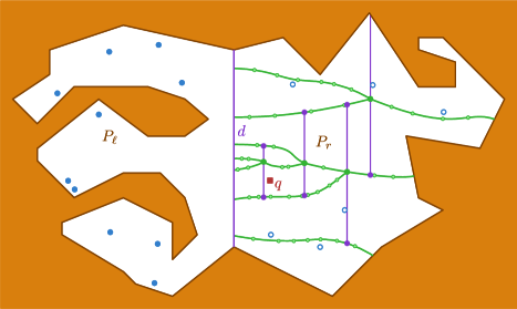
Figure 1: A sketch of the global approach. The diagonal $d$ splits $P$ into $P_{\ell}$ and $P_{r}$. The $k$ sites in $P_{\ell}$ induce a forest $\mathcal{V}$ in $P_{r}$ with $O(k)$ degree three nodes, but potentially $O(m)$ degree two nodes. Using $\mathcal{V}$ we can locate the site closest to $q$ among the sites in $P_{\ell}$.

The Global Approach.

The general idea in our approach is to recursively partition the polygon into two roughly equal size sub-polygons $P_{\ell}$ and $P_{r}$ that are separated by a diagonal. Additionally, we partition the sites that lie in $P_{\ell}$ into a small number of subsets. The Voronoi diagram that such a subset $S^{*}$ induces in the other half of the polygon, $P_{r}$, is a forest $\mathcal{V}$. See Fig. 1 for an illustration. We show that we can efficiently construct a compact representation of this forest that supports planar point location queries. We handle the sites that lie in $P_{r}$ analogously. When we get a query point $q\in P_{r}$, our forests allow us to find the site in $P_{\ell}$ closest to $q$ efficiently. To find the site in $P_{r}$ closest to $q$, we recursively query in sub-polygon $P_{r}$. When we add or remove a site $s$ we have to rebuild the forests associated with only few subsets containing $s$. We show that we can recompute each forest $\mathcal{V}$ efficiently.

We give a more detailed description of the approach in Section 2. The core of our solution is that we can represent, and construct, the Voronoi diagram $\mathcal{V}$ that a set of sites $S^{*}$ in $P_{\ell}$ induces in $P_{r}$ in time proportional to the size $k$ of the subset $S^{*}$. In particular, our representation has a size $O(k)$ and can be built in time $O(k\log^{2}m)$. We show this in Section 4. The key to achieving this result is a representation of the bisector $b_{st}$ of two sites $s$ and $t$. Our representation of $b_{st}$, presented in Section 3, allows us to find the intersection of $b_{st}$ with another bisector $b_{tu}$ in $P_{r}$ efficiently, and can be obtained from the input polygon in $O(\log^{2}m)$ time. We combine all of the components into a fully dynamic data structure in Section 5. Furthermore, we show that we can get improved query and update times in the insertion-only and offline-cases.

2 An Overview of the Data Structure

As in previous work on geodesic Voronoi diagrams [2, 20], we assume that $P$ and $S$ are in general position. That is, (i) no two sites $s$ and $t$ in $S$ (ever) have the same geodesic distance to a vertex of $P$, and (ii) no three points (either sites or vertices) are colinear. Note that (i) implies that no bisector $b_{st}$ between sites $s$ and $t$ contains a vertex of $P$.

We start by preprocessing $P$ for two-point shortest path queries using the data structure by Guibas and Hershberger [10] (see also the follow up note of Hershberger [11]). This takes $O(m)$ time and allows us to compute the geodesic distance $\scaleobj{1.7}{\varsigma}(p,q)$ between any pair of query points $p,q\in P$ in $O(\log m)$ time. We then construct a balanced decomposition of $P$ into sub-polygons [9]. A balanced decomposition is a binary tree in which each node represents a sub-polygon $P^{\prime}$ of $P$, together with a diagonal $d$ of $P^{\prime}$ that splits $P^{\prime}$ into two sub-polygons $P_{\ell}$ and $P_{r}$ that have roughly the same number of vertices. As a result, the height of the tree, and thus the number of levels in the decomposition, is $O(\log m)$. The root of the tree represents the polygon $P$ itself.

Consider a diagonal $d$ of $P^{\prime}$ that splits $P^{\prime}$ into $P_{\ell}$ and $P_{r}$, and let $S_{\ell}=S\cap P_{\ell}$ denote the set of sites in $P_{\ell}$. The Voronoi diagram of $S_{\ell}$ in $P_{r}$ is a forest with $O(k)$, where $k=|S_{\ell}|$, nodes of degree one or three, and $O(m)$ nodes of degree two [2]. The degree three nodes correspond to intersection points of two bisectors, and the degree one nodes correspond to intersection points of a bisector with the polygon boundary. See Fig. 1 for an illustration. We refer to the topological structure of the forest, i.e. the forest with only the degree one and three nodes, of $S_{\ell}$ as $\mathcal{V}$.

At every level of the decomposition, we partition the sites in $S_{\ell}$ in $O(\sqrt{n})$ subsets, each of size $O(\sqrt{n})$. For each subset $S^{*}$ we explicitly build the embedded forest $\mathcal{V}$ that represents its Voronoi diagram in $P_{r}$ using an algorithm for constructing a Hamiltonian abstract Voronoi diagram [15]. More specifically, for every degree one or three node, we compute the location of the intersection point that it is representing, and to which other nodes (of degree one or three) it is connected to. Furthermore, we preprocess $\mathcal{V}$ for planar point location. Note that the edges in this planar subdivision correspond to pieces of bisectors, and thus are actually chains of hyperbolic arcs, each of which may have a high internal complexity. We do not explicitly construct these chains, but show that there is an oracle that can decide if a query point $q\in P_{r}$ lies above or below a chain (edge of the planar subdivision) in $O(\log m)$ time. It follows that our representation of $\mathcal{V}$ has size $O(k)$, where $k=|S^{*}|$, and supports planar point location queries in $O(\log k\log m)$ time. We handle the sites $S_{r}=S\cap P_{r}$ in $P_{r}$ analogously.

Once $P^{\prime}$ is a triangle, corresponding to a leaf in the balanced decomposition, the geodesic between any pair of points in $P^{\prime}$ is a single line segment, and thus the geodesic distance equals the Euclidean distance. In this case, we maintain the sites in $P^{\prime}$ in a dynamic Euclidean nearest neighbor data structure such as the one of Chan [5] or the much simpler data structure of Bentley and Saxe [3].

Since every site $s$ is stored in exactly one subset at every level of the decomposition, and the Voronoi diagram for each such subset has linear size, the data structure uses $O(n\log m+m)$ space.

Handling a Query.

Consider a nearest neighbor query with point $q\in P^{\prime}$ at a node of the balanced decomposition corresponding to sub-polygon $P^{\prime}$, and let $P_{\ell}$ and $P_{r}$ be the sub-polygons into which $P^{\prime}$ is split. In case that $q\in P_{r}$, we find the site $s$ in $P_{\ell}$ closest to $q$, and recursively query the data structure for the nearest neighbor of $q$ in sub-polygon $P_{r}$. We handle the case that $q\in P_{\ell}$ analogously. Once $P^{\prime}$ is a triangle we find the site closest to $q$ by querying the Euclidean nearest neighbor searching data structure associated with $P^{\prime}$. For each of the $O(\log m)$ levels of the balanced decomposition this gives us a candidate closest site, and we return the one that is closest over all.

Since we partitioned the set of sites $S_{\ell}$ that lie in $P_{\ell}$ into $O(\sqrt{n})$ subsets, we can find the site $s\in S_{\ell}$ closest to $q$ by a point location query in the Voronoi diagram associated with each of these subsets. Each such a query takes $O(\log n\log m)$ time, and thus we can find $s$ in $O(\sqrt{n}\log n\log m)$. The final query in the Euclidean nearest neighbor data structure can easily be handled in $O(\sqrt{n}\log n)$ time [3]. Since we have $O(\log m)$ levels in the balanced decomposition, the total query time is $O(\sqrt{n}\log n\log^{2}m)$.

Handling Updates.

Consider inserting a new site $s$ into the data structure, or removing $s$ from $S$. The site $s$ needs to be, or is, stored in exactly one subset at every level of the decomposition. Suppose that $s$ needs to be, or is, in the subset $S^{*}$ of $S_{\ell}$ at some level of the decomposition. We then simply rebuild the forest $\mathcal{V}$ associated with $S^{*}$. In Section 4 we will show that we can do this in $O(|\mathcal{V}|\log^{2}m)$ time. Since the subset containing $s$, and thus its corresponding forest $\mathcal{V}$, has size $O(\sqrt{n})$, the cost per level is $O(\sqrt{n}\log^{2}m)$. Inserting $s$ into or deleting $s$ from the final Euclidean nearest neighbor data structure can be done in $O(\sqrt{n})$ time [3]. It follows that the total update time is $O(\sqrt{n}\log^{3}m)$.

3 Representing a Bisector

Assume without loss of generality that the diagonal $d$ that splits $P$ into $P_{\ell}$ and $P_{r}$ is a vertical line-segment, and let $s$ and $t$ be two sites in $S_{\ell}$. In this section we show that there is a representation of $b^{*}_{st}=b_{st}\cap P_{r}$, the part of the bisector $b_{st}$ that lies in $P_{r}$, that allows efficient random access to the bisector vertices. Moreover, we can obtain such a representation using a slightly modified version of the two-point shortest path data structure of Guibas and Hershberger [10].

Let $s$ be a site in $S_{\ell}$, and consider the shortest path tree $T$ rooted at $s$. Let $e=\overline{uv}$ be an edge of $T$ for which $v$ is further away from $s$ than $u$. The half-line starting at $v$ that is colinear with, and extending $e$ has its first intersection with the boundary $\partial P$ of $P$ in a point $w$. We refer to the segment $\overline{vw}$ as the extension segment of $v$ [2]. Let $E_{s}$ denote the set of all extension segments of all vertices in $T$.

Figure 2: (a) The polygon $\mathcal{P}(p,s,t)$ bounded by the shortest paths between $s$, $p$, and $t$ is a pseudo-triangle $\hat{\mathcal{P}}(p,s,t)$ with polylines attached to its corners $\hat{s}$, $\hat{p}$, and $\hat{t}$. It contains the funnel $\mathcal{F}(p,s,t)$. (b) The clipped extension segments in $F_{s}^{t}$ are all pairwise disjoint, and end at the chain from $t$ to $z$.

Consider two sites $s,t\in S_{\ell}$, and its bisector $b_{st}$. We then have

Lemma 1 (Lemma 3.22 of Aronov [2]).

The bisector $b_{st}$ is a smooth curve connecting two points on $\partial P$ and having no other points in common with $\partial P$. It is the concatenation of $O(m)$ straight and hyperbolic arcs. The points along $b_{st}$ where adjacent pairs of these arcs meet, i.e., the vertices of $b_{st}$, are exactly the intersections of $b_{st}$ with the segments of $E_{s}$ or $E_{t}$.

Lemma 2 (Lemma 3.28 of Aronov [2]).

For any point $p\in P$, the bisector $b_{st}$ intersects the shortest path $\scaleobj{1.15}{\varsigma}(s,p)$ in at most a single point.

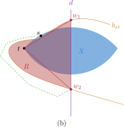
Figure 3: The geodesic distance from $t$ to $w_{1}$ and $w_{2}$ equals its Euclidean distance. The shortest path from $s$ to $w_{2}$ (dashed, green) has to go around $R$, and is thus strictly longer than $\|tw_{2}\|$.

Consider a point $p$ on $\partial P_{r}$ and let $\mathcal{P}(p,s,t)$ be the polygon defined by the shortest paths $\scaleobj{1.15}{\varsigma}(s,p)$, $\scaleobj{1.15}{\varsigma}(p,t)$, and $\scaleobj{1.15}{\varsigma}(t,s)$. This polygon $\mathcal{P}(p,s,t)$ is a pseudo-triangle $\hat{\mathcal{P}}(p,s,t)$ whose corners $\hat{s}$, $\hat{t}$, and $\hat{p}$, are connected to $s$, $t$, and $p$ respectively, by arbitrary polylines.

Let $s^{\prime}$ and $t^{\prime}$ be the intersection points between $d$ and the geodesics $\scaleobj{1.15}{\varsigma}(p,s)$ and $\scaleobj{1.15}{\varsigma}(p,t)$, respectively, and assume without loss of generality that $s^{\prime}_{y}\leq t^{\prime}_{y}$. The restriction of $\mathcal{P}(p,s,t)$ to $P_{r}$ is a funnel $\mathcal{F}(p,s,t)$, bounded by $\scaleobj{1.15}{\varsigma}(t^{\prime},p)$, $\scaleobj{1.15}{\varsigma}(p,s^{\prime})$, and $\overline{s^{\prime}t^{\prime}}$. See Fig. 2(a). Note that $\scaleobj{1.15}{\varsigma}(s,t)$ is contained in $P_{\ell}$.

Clearly, if $b_{st}$ intersects $P_{r}$ then it intersects $d$. There is at most one such intersection point:

Lemma 3.

The bisector $b_{st}$ intersects $d$ in at most one point $w$.

Proof.

Assume, by contradiction, that $b_{st}$ intersects $d$ in two points $w_{1}$ and $w_{2}$, with $w_{1}$ above $w_{2}$. See Fig. 3(b). Note that by Lemma 1, $b_{st}$ cannot intersect $\partial P_{\ell}$, and thus $d$, in more than two points. Thus, the part of $b_{st}$ that lies in $P_{\ell}$ between $w_{1}$ and $w_{2}$ does not intersect $\partial P_{\ell}$. Observe that this implies that the region $R$ enclosed by this part of the curve, and the part of the diagonal from $w_{1}$ to $w_{2}$ (i.e. $\overline{w_{1}w_{2}}$) is empty. Moreover, since the shortest paths from $t$ to $w_{1}$ and to $w_{2}$ intersect $b_{st}$ only once (Lemma 2) region $R$ contains the shortest paths $\scaleobj{1.15}{\varsigma}(t,w_{1})=\overline{tw_{1}}$ and $\scaleobj{1.15}{\varsigma}(t,w_{2})=\overline{tw_{2}}$.

Since $s$ has the same geodesic distance to $w_{1}$ and $w_{2}$ as $t$, $s$ must lie in the intersection $X$ of the disks $D_{i}$ with radius $\|tw_{i}\|$ centered at $w_{i}$, for $i\in 1,2$. It now follows that $s$ lies in one of the connected sets, or “pockets”, of $X\setminus R$. Assume without loss of generality that it lies in a pocket above $t$ (i.e. $s_{y}>t_{y}$). See Fig. 3. We now again use Lemma 2, and get that $\scaleobj{1.15}{\varsigma}(s,w_{2})$ intersects $b_{st}$ only once, namely in $w_{2}$. It follows that the shortest path from $s$ to $w_{2}$ has to go around $R\ni t$, and thus has length strictly larger than $\|tw_{2}\|$. Contradiction. ∎

Since $b_{st}$ intersects $d$ only once (Lemma 3), and there is a point of $b_{st}$ on $\scaleobj{1.15}{\varsigma}(s,t)\subset P_{\ell}$, it follows that there is at most one point $z$ where $b_{st}$ intersects $\partial P_{r}$ the outer boundary of $P_{r}$, i.e. $\partial P_{r}\setminus d$. Observe that therefore $z$ is a corner of the pseudo-triangle $\hat{\mathcal{P}}(z,s,t)$, and that $\mathcal{F}(z,s,t)\subseteq\hat{\mathcal{P}}(z,s,t)$. Let $b^{*}_{st}=b_{st}\cap P_{r}$ and orient it from $w$ to $z$. We assign $b_{st}$ the same orientation.

Lemma 4.

(i) The bisector $b_{st}$ does not intersect $\scaleobj{1.15}{\varsigma}(s,z)$ or $\scaleobj{1.15}{\varsigma}(t,z)$ in any point other than $z$. (ii) The part of the bisector $b_{st}$ that lies in $P_{r}$ is contained in $\mathcal{F}(z,s,t)$.

Proof.

By Lemma 2 the shortest path from $s$ to any point $v\in P$, so in particular to $z$, intersects $b_{st}$ in at most one point. Since, by definition, $z$ lies on $b_{st}$, the shortest path $\scaleobj{1.15}{\varsigma}(s,z)$ does not intersect $b_{st}$ in any other point. The same applies for $\scaleobj{1.15}{\varsigma}(t,z)$, thus proving (i). For (ii) we observe that any internal point of $\scaleobj{1.15}{\varsigma}(s,z)$ is closer to $s$ than to $t$, and any internal point of $\scaleobj{1.15}{\varsigma}(t,z)$ closer to $t$ than to $s$. Thus, $\scaleobj{1.15}{\varsigma}(s,z)$ and $\scaleobj{1.15}{\varsigma}(t,z)$ must be separated by $b_{st}$. It follows that $b_{st}\cap P_{r}$ lies inside $\mathcal{F}(z,s,t)$. ∎

Lemma 5.

All vertices of $b^{*}_{st}$ lie on extension segments of the vertices in the pseudo-triangle $\hat{\mathcal{P}}(z,s,t)$.

Proof.

Assume by contradiction that $v\neq w$ is a vertex of $b^{*}_{st}=b_{st}\cap P_{r}$ that is not defined by an extension segment of a vertex in $\hat{\mathcal{P}}(z,s,t)$. Instead, let $e\in E_{s}$ be the extension segment containing $v$, and let $u\in P\setminus\hat{\mathcal{P}}(z,s,t)$ be the starting vertex of $e$. So $\scaleobj{1.15}{\varsigma}(s,v)$ has $u$ as its last internal vertex.

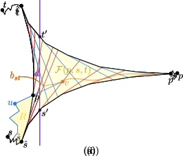
Figure 4: (a) Point $v$ lies inside $\hat{\mathcal{P}}(z,s,t)$, so a shortest path from $s$ to $v$ that uses a vertex $u$ outside of $\hat{\mathcal{P}}(z,s,t)$ intersects $\partial\hat{\mathcal{P}}(z,s,t)$ in a point $p$. This either yields two distinct shortest paths from $s$ to $p$, or requires the shortest path from $s$ to $p$ via $u$ to intersect $b_{st}$ twice. Both yield a contradiction. (b) The extension segments in $F_{s}^{t}$ are all pairwise disjoint, and end at the chain from $t$ to $z$.

By Lemma 4, $b^{*}_{st}$ is contained in $\mathcal{F}(z,s,t)$ and thus in $\hat{\mathcal{P}}(z,s,t)$. Hence, $v\in\hat{\mathcal{P}}(z,s,t)$. Since $v\in\hat{\mathcal{P}}(z,s,t)$, and $u\not\in\hat{\mathcal{P}}(z,s,t)$ the shortest path from $s$ to $v$ intersects $\partial\hat{\mathcal{P}}(z,s,t)$ in some point $p$. See Fig. 4(a). We then distinguish two cases: either $p$ lies on $\scaleobj{1.15}{\varsigma}(s,z)\cup\scaleobj{1.15}{\varsigma}(s,t)$, or $p$ lies on $\scaleobj{1.15}{\varsigma}(t,z)$.

In the former case this means there are two distinct shortest paths between $s$ and $p$, that bound a region $R$ that is non-empty, that is, it has positive area. Note that this region exists, even if $u$ lies on the shortest path from $s$ to its corresponding corner $\hat{s}$ in $\hat{\mathcal{P}}(z,s,t)$ but not on $\hat{\mathcal{P}}(z,s,t)$ itself (i.e. $u\in\scaleobj{1.15}{\varsigma}(s,t)\cup\scaleobj{1.15}{\varsigma}(s,z)\setminus\hat{\mathcal{P}}(z,s,t)$. Since $P$ is a simple polygon, this region $R$ is empty of obstacles, and we can shortcut one of the paths to $p$. This contradicts that such a path is a shortest path.

In the latter case the point $p$ lies on $\scaleobj{1.15}{\varsigma}(t,z)$, which means that it is at least as close to $t$ as it is to $s$. Since $s$ is clearly closer to $s$ than to $t$, this means that the shortest path from $s$ to $v$ (that visits $u$ and $p$) intersects $b_{st}$ somewhere between $s$ and $p$. Since it again intersects $b_{st}$ at $v$, we now have a contradiction: by Lemma 2, any shortest path from $s$ to $v$ intersects $b_{st}$ at most once. The lemma follows. ∎

Let $F_{s}^{t}=e_{1},..,e_{g}$ denote the extension segments of the vertices of $\scaleobj{1.15}{\varsigma}(t,s)$ and $\scaleobj{1.15}{\varsigma}(s,z)$, ordered along $\hat{\mathcal{P}}(z,s,t)$, and clipped to $\hat{\mathcal{P}}(z,s,t)$. See Fig. 2(b). We define $F_{t}^{s}$ analogously.

Lemma 6.

All vertices of $b^{*}_{st}$ lie on clipped extension segments in $F_{s}^{t}\cup F_{t}^{s}$.

Proof.

By Lemma 5 all vertices of $b_{st}$ in $P_{r}$ lie on $\hat{\mathcal{P}}(z,s,t)$. Furthermore, by Lemma 4 all these vertices lie in $\mathcal{F}(z,s,t)$. Hence, it suffices to clip all extension segments to $\hat{\mathcal{P}}(z,s,t)$ (or even $\mathcal{F}(z,s,t)$). For all vertices on $\scaleobj{1.15}{\varsigma}(t,z)$ the extension segments (with respect to $s$) are disjoint from $\hat{\mathcal{P}}(z,s,t)$. It follows that for site $s$, only the clipped extension segments from vertices on $\scaleobj{1.15}{\varsigma}(s,t)$ and $\scaleobj{1.15}{\varsigma}(s,z)$ are relevant. Analogously, for site $t$, only the clipped extension segments on $\scaleobj{1.15}{\varsigma}(s,t)$ and $\scaleobj{1.15}{\varsigma}(t,z)$ are relevant. ∎

Observation 7.

The extension segments in $F_{s}^{t}$ are all pairwise disjoint, start on $\scaleobj{1.15}{\varsigma}(s,t)$ or $\scaleobj{1.15}{\varsigma}(s,z)$, and end on $\scaleobj{1.15}{\varsigma}(t,z)$.

Figure 5: The extension segments in $F_{s}^{t}$ are all pairwise disjoint, and end at the chain from $t$ to $z$.

By Corollary 3.29 of Aronov [2] every (clipped) extension segment in $r\in F_{s}^{t}\cup F_{t}^{s}$ intersects $b_{st}$ (and thus $b^{*}_{st}$) at most once. Therefore, every such extension segment $r$ splits the bisector in two. Together with Lemma 6 and Observation 7 this now give us sufficient information to efficiently binary search among the vertices of $b^{*}_{st}$ when we have (efficient) access to $\hat{\mathcal{P}}(z,s,t)$.

Lemma 8.

Consider extension segments $e_{i}$ and $e_{j}$, with $i\leq j$, in $F_{s}^{t}$. If $e_{i}$ intersects $b_{st}$ then so does $e_{j}$.

Proof.

It follows from Lemma 4 that $b_{st}$ intersects $\partial\hat{\mathcal{P}}(z,s,t)$ only in $z$ and in a point $w^{\prime}$ on $\scaleobj{1.15}{\varsigma}(s,t)$. Thus, $b_{st}$ partitions $\hat{\mathcal{P}}(z,s,t)$ into an $s$-side, containing $\scaleobj{1.15}{\varsigma}(s,z)$, and a $t$-side, containing $\scaleobj{1.15}{\varsigma}(t,z)$. Since the extension segments also partition $\hat{\mathcal{P}}(z,s,t)$ it then follows that the extension segments in $F_{s}^{t}$ intersect $b_{st}$ if and only if their starting point lies in the $s$-side and their ending point lies in the $t$-side. By Observation 7 all segments in $F_{s}^{t}$ end on $\scaleobj{1.15}{\varsigma}(t,z)$. Hence, they end on the $t$-side. We finish the proof by showing that if $e_{i}\in F_{s}^{t}$ starts on the $s$-side, so must $e_{j}\in F_{s}^{t}$, with $j\geq i$.

The extension segments of vertices in $\scaleobj{1.15}{\varsigma}(s,z)$ trivially have their start point on the $s$-side. It thus follows that they all intersect $b_{st}$. For the extension segments of vertices in $\scaleobj{1.15}{\varsigma}(s,t)$ the ordering is such that the distance to $s$ is monotonically decreasing. Hence, if $e_{i}$ intersects $b_{st}$, and thus starts on the $s$-side, so does $e_{j}$, with $j\geq i$. ∎

Lemma 9.

Consider extension segments $e_{i}$ and $e_{j}$, with $i\leq j$, in $F_{s}^{t}$. If $e_{i}$ intersects $b^{*}_{st}$ then so does $e_{j}$.

Proof.

From Lemma 8 it follows that if $e_{i}$ intersects $b_{st}$ then so does $e_{j}$, with $j\geq i$. So, we only have to show that if $e_{i}$ intersects $b_{st}$ in $P_{r}$ then so does $e_{j}$. Since the extension segments in $F_{s}^{t}$ are pairwise disjoint, it follows that if $e_{i}$ intersects $b_{st}$, say in point $p$ then $e_{j}$, with $j\geq i$ must intersect $b_{st}$ on the subcurve between $p$ and $z$. Since $b_{st}$ intersects $d$ at most once (Lemma 3), and $p\in P_{r}$, it follows that this part of the curve, and thus its intersection with $e_{j}$, also lies in $P_{r}$. ∎

Corollary 10.

The segments in $F_{s}^{t}$ that define a vertex in $b^{*}_{st}$ form a suffix $G_{s}^{t}$ of $F_{s}^{t}$. That is, there is an index $a$ such that $G_{s}^{t}=e_{a},..,e_{g}$ is exactly the set of extension segments in $F_{s}^{t}$ that define a vertex of $b^{*}_{st}$.

When we have $\hat{\mathcal{P}}(z,s,t)$ and the point $w$, we can find the value $a$ from Corollary 10 in $O(\log m)$ time as follows. We binary search along $\scaleobj{1.15}{\varsigma}(t,s)$ to find the first vertex $u_{a^{\prime}}$ such that $u_{a^{\prime}}$ is closer to $s$ then to $t$. For all vertices after $u_{a^{\prime}}$, its extension segment intersects $b_{st}$ in $\hat{\mathcal{P}}(z,s,t)$. To find the first segment that intersects $b_{st}$ in $P_{r}$, we find the first index $a\geq a^{\prime}$ for which the extension segment intersects $d$ below $w$. In total this takes $O(\log m)$ time.

Figure 6: The bisector vertex $v_{c}$ on $f_{j}$ occurs before $v_{d}$ on $r_{i}$.

Let $G_{s}^{t}=r_{1},..,r_{g^{\prime}}=e_{a},..,e_{g}$ be the ordered set of extension segments that intersect $b^{*}_{st}$. Similarly, let $G_{t}^{s}=f_{1},..,f_{h^{\prime}}$ be the suffix of extension segments from $F_{t}^{s}$ that define a vertex of $b^{*}_{st}$.

Observation 11.

Let $r_{i}$ be an extension segment in $G_{s}^{t}$, and let $v_{d}$ be the vertex of $b_{st}$ on $r_{i}$. Let $f_{j}$ be the last extension segment in $G_{t}^{s}$ such that $f_{j}$ intersects $r_{i}$ in a point closer to $s$ than to $t$. See Fig. 6. The vertex $v_{c}$ of $b_{st}$ corresponding to $f_{j}$ occurs before $v_{d}$, that is $c<d$.

Proof.

By definition of $j$ it follows that the intersection point $v_{d}$ of $r_{i}$ and $b^{*}_{st}$ lies between the intersection of $r_{i}$ with $f_{j}$ and $f_{j+1}$. See Fig. 6. Thus, the intersection point ∎

Lemma 12.

Let $j$ be the number of extension segments in $G_{t}^{s}$ that intersect $r_{i}$ in a point closer to $s$ than to $t$. Then $r_{i}$ contains vertex $v_{d}=v_{i+j}$ of $b^{*}_{st}$.

Proof.

It follows from Corollary 10 and the definition of $G_{s}^{t}$ and $G_{t}^{s}$ that all vertices of $b^{*}_{st}$ lie on extension segments in $\{r_{1},..,r_{g^{\prime}}\}\cup\{f_{1},..,f_{h^{\prime}}\}$. Together with Corollary 3.29 of Aronov [2] we get that every such extension segment defines exactly one vertex of $b^{*}_{st}$. Since the bisector intersects the segments $r_{1},..,r_{g^{\prime}}$ in order, there are exactly $i-1$ vertices of $b^{*}_{st}$ before $v_{d}$, defined by the extension segments in $G_{s}^{t}$. Let $f_{\ell}$ be the last extension segment in $G_{t}^{s}$ that intersects $r_{i}$ in a point closer to $s$ than to $t$. Observation 11 gives us that this extension segment defines a vertex $v_{c}$ of $b_{st}$ with $c<d$. We then again use that $b^{*}_{st}$ intersects the segments $f_{1},..,f_{h^{\prime}}$ in order, and thus $\ell=j$. Hence, $v_{d}$ is the $(i+j)^{\text{th}}$ vertex of $b^{*}_{st}$. ∎

It follows from Lemma 12 that if we have $\hat{\mathcal{P}}(z,s,t)$ and we have efficient random access to its vertices, we also have efficient access to the vertices of the bisector $b^{*}_{st}$. Next, we argue with some minor augmentations the preprocessing of $P$ into a two-point query data structure by Guibas and Hershberger gives us such access.

Accessing $\hat{\mathcal{P}}(z,s,t)$.

The data structure of Guibas and Hershberger can return the shortest path between two query points $p$ and $q$, represented as a balanced tree [10, 11]. This tree is essentially a persistent balanced search tree on the edges of the path. Every node of the tree can access an edge $e$ of the path in constant time, and the edges are stored in order along the path. The tree is balanced, and supports concatenating two paths efficiently. To support random access to the vertices of $\hat{\mathcal{P}}(z,s,t)$ we need two more operations: we need to be able to access the $i^{\text{th}}$ edge or vertex in a path, and we need to be able to find the longest prefix (or suffix) of a shortest path that forms a convex chain. This last operation will allow us to find the corners $\hat{s}$ and $\hat{t}$ of $\hat{\mathcal{P}}(z,s,t)$. The data structure as represented by Guibas and Hershberger does not support these operations directly. However, with two simple augmentations we can support them in $O(\log m)$ time. In the following, we use the terminology as used by Guibas and Hershberger [10].

The geodesic between $p$ and $q$ is returned as a balanced tree. The leaves of this tree correspond to, what Guibas and Hershberger call, fundamental strings: two convex chains joined by a tangent. The individual convex chains are stored as balanced binary search trees. The internal nodes have two or three children, and represent derived strings: the concatenation of the fundamental strings stored in its descendant leaves. See Fig. 7 for an illustration.

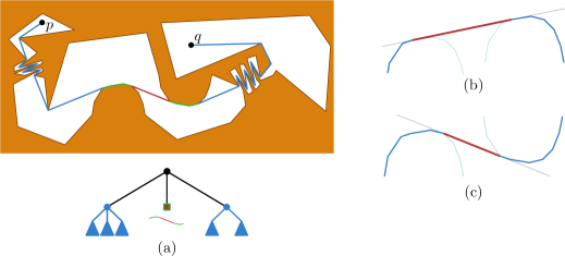
Figure 7: The data structure of Guibas and Hershberger [10] can return the geodesic between two query points $p$ and $q$ as a balanced tree (a). The leaves of the tree correspond to fundamental strings: two convex chains joined by a tangent. The internal nodes represent derived strings: the concatenation of two or three sub-paths (strings). A fundamental string can be convex (b) or non-convex (c).

To make sure that we can access the $i^{\text{th}}$ vertex or edge on a shortest path in $O(\log m)$ time, we augment the trees to store subtree sizes. It is easy to see that we can maintain these subtree sizes without affecting the running time of the other operations.

To make sure that we can find the longest prefix (suffix) of a shortest path that is convex we do the following. With each node $v$ in the tree we store a boolean flag $v\mathit{.convex}$ that is true if and only if the sub path it represents forms a convex chain. It is easy to maintain this flag without affecting the running time of the other operations. For leaves of the tree (fundamental strings) we can test this by checking the orientation of the tangent with its two adjacent edges of its convex chains. These edges can be accessed in constant time. Similarly, for internal nodes (derived strings) we can determine if the concatenation of the shortest paths represented by its children is convex by inspecting the $\mathit{convex}$ field of its children, and checking the orientation of only the first and last edges of the shortest paths. We can access these edges in constant time. This augmentation allows us to find the last vertex $v$ of a shortest path $\scaleobj{1.15}{\varsigma}(p,q)$ such that $\scaleobj{1.15}{\varsigma}(p,v)$ is a convex chain in $O(\log m)$ time. We can then obtain $\scaleobj{1.15}{\varsigma}(p,v)$ itself (represented by a balanced tree) in $O(\log m)$ time by simply querying the data structure with points $p$ and $v$. Hence, we can compute the longest prefix (or suffix) on which a shortest path forms a convex chain in $O(\log m)$ time.

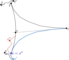
Figure 8: We can find the first point $s^{\prime}$ on $\scaleobj{1.15}{\varsigma}(s,z)$ such that $\scaleobj{1.15}{\varsigma}(s^{\prime},z)$ is convex. When we have a point $v$ of $\scaleobj{1.15}{\varsigma}(s^{\prime},t^{\prime})$ known to be in $\hat{\mathcal{P}}(z,s,t)$, we can find $s^{\prime\prime}=\hat{s}$ (darkblue). The first point $s^{\prime\prime}$ on $\scaleobj{1.15}{\varsigma}(s^{\prime},t^{\prime})$ such that $\scaleobj{1.15}{\varsigma}(s^{\prime\prime},v)$ is convex has to lie on $\scaleobj{1.15}{\varsigma}(s^{\prime},z)$. If this is not the case (as shown in red), then we can shortcut the shortest path to avoid $s^{\prime\prime}$, leading to a contradiction.

Given point $z$, the above augmentation allow us to access $\hat{\mathcal{P}}(z,s,t)$ in $O(\log m)$ time. We query the data structure to get the tree representing $\scaleobj{1.15}{\varsigma}(s,z)$, and, using our augmentations, find the longest convex suffix $\scaleobj{1.15}{\varsigma}(s^{\prime},z)$. Similarly, we find the longest convex suffix $\scaleobj{1.15}{\varsigma}(t^{\prime},z)$ of $\scaleobj{1.15}{\varsigma}(t,z)$. Observe that the corners $\hat{s}$ and $\hat{t}$ of $\hat{\mathcal{P}}(z,s,t)$ lie on $\scaleobj{1.15}{\varsigma}(s^{\prime},z)$ and $\scaleobj{1.15}{\varsigma}(t^{\prime},z)$, respectively (otherwise $\scaleobj{1.15}{\varsigma}(\hat{s},z)$ and $\scaleobj{1.15}{\varsigma}(\hat{t},z)$ would not be convex chains). Unfortunately, we cannot directly use the same approach to find the part $\scaleobj{1.15}{\varsigma}(s^{\prime},t^{\prime})$ that is convex, as it may both start and end with a piece that is non-convex (with respect to $\scaleobj{1.15}{\varsigma}(s^{\prime},t^{\prime})$). However, consider the extension segment of the first edge of the shortest path from $z$ to $s$ (see Fig. 8). This extension segment intersects the shortest path $\scaleobj{1.15}{\varsigma}(s^{\prime},t^{\prime})$ exactly once in a point $v$. By construction, this point $v$ must lie in the pseudo-triangle $\hat{\mathcal{P}}(z,s,t)$. Thus, we can decompose $\scaleobj{1.15}{\varsigma}(s^{\prime},t^{\prime})$ into two sub-paths, one of which starts with a convex chain and the other ends with a convex chain. Hence, for those chains we can use the $\mathit{convex}$ fields to find the vertices $s^{\prime\prime}$ and $t^{\prime\prime}$ such that $\scaleobj{1.15}{\varsigma}(s^{\prime\prime},v)$ and $\scaleobj{1.15}{\varsigma}(v,t^{\prime\prime})$ are convex, and thus $\scaleobj{1.15}{\varsigma}(s^{\prime\prime},t^{\prime\prime})$ is convex. Finally, observe that $s^{\prime\prime}$ must occur on $\scaleobj{1.15}{\varsigma}(s^{\prime},z)$, otherwise we could shortcut $\scaleobj{1.15}{\varsigma}(s^{\prime},t^{\prime})$. See Fig. 8. Hence, $s^{\prime\prime}=\hat{s}$ and $t^{\prime\prime}=\hat{t}$ are the two corners of the pseudo-triangle $\hat{\mathcal{P}}(z,s,t)$. We can find $v$ in $O(\log m)$ time by a binary search on $\scaleobj{1.15}{\varsigma}(s^{\prime},t^{\prime})$. Finding the longest convex chains starting and ending in $v$ also takes $O(\log m)$ time, as does computing the shortest path $\scaleobj{1.15}{\varsigma}(\hat{s},\hat{t})$. It follows that given $z$, we can compute (a representation of) $\hat{\mathcal{P}}(z,s,t)$ in $O(\log m)$ time.

With the above augmentations, and using Lemma 12, we then obtain the following result.

Lemma 13.

Given the points $w$ and $z$ where $b^{*}_{st}$ intersects $d$ and the outer boundary of $P_{r}$, respectively, we can access the $i^{\text{th}}$ vertex of $b^{*}_{st}$ in $O(\log m)$ time.

Proof.

Recall that the data structure of Guibas and Hershberger [10] reports the shortest path between query points $p$ and $q$ as a balanced tree. We augment these trees such that each node knows the size of its subtree. It is easy to do this using only constant extra time and space, and without affecting the other operations. We can then simply binary search on the subtree sizes, using Lemma 12 to guide the search. ∎

Finding $w$ and $z$.

We first show that we can find the point $w$ where $b_{st}$ enters $P_{r}$ (if it exists), and then show how to find $z$, the other point where $b_{st}$ intersects $\partial P_{r}$.

Lemma 14.

We can find $w$ in $O(\log^{2}m)$ time.

Proof.

Consider the geodesic distance of $s$ to diagonal $d$ as a function $f_{s}$, parameterized by a value $\lambda\in[0,1]$ along $d$. Similarly, let $f_{t}$ be the distance function from $t$ to $d$. Since $b_{st}$ intersects $d$ exactly once –namely in $w$– the predicate $\hat{\mathcal{P}}(\lambda)=f_{s}(\lambda)<f_{t}(\lambda)$ changes from True to False (or vice versa) exactly once. Query the data structure of Guibas and Hershberger [10] to get the funnel representing the shortest paths from $s$ to the points in $d$. Let $p_{1},..,p_{h}$, with $h=O(m)$, be the intersection points of the extension segments of vertices in the funnel with $d$. Similarly, compute the funnel representing the shortest paths from $t$ to $d$. The extension segments in this funnel intersect $d$ in points $q_{1},..,q_{k}$, with $k=O(m)$. We can now simultaneously binary search among $p_{1},..,p_{h}$ and $q_{1},..,q_{k}$ to find the smallest interval $I$ bounded by points in $\{p_{1},..,p_{h},q_{1},..,q_{k}\}$ in which $\hat{\mathcal{P}}$ flips from True to False. Hence, $I$ contains $w$. Computing the distance from $s$ ($t$) to some $q_{i}$ ($p_{i}$) takes $O(\log m)$ time, and thus we can find $I$ in $O(\log^{2}m)$ time. On interval $I$ both $f_{s}$ and $f_{t}$ are simple hyperbolic functions consisting of a single piece, and thus we can compute $w$ in constant time. ∎

Consider the vertices $v_{1},..,v_{h}$ of $P_{r}$ in clockwise order, where $d=\overline{v_{h}v_{1}}$ is the diagonal. Since the bisector $b_{st}$ intersects the outer boundary of $P_{r}$ in only one point, there is a vertex $v_{a}$ such that $v_{1},..,v_{a}$ are all closer to $t$ than to $s$, and $v_{a+1},..,v_{h}$ are all closer to $s$ than to $t$. We can thus find this vertex $v_{a}$ using a binary search. This takes $O(\log^{2}m)$ time, as we can compute $\scaleobj{1.7}{\varsigma}(s,v_{i})$ and $\scaleobj{1.7}{\varsigma}(t,v_{i})$ in $O(\log m)$ time. It then follows that $z$ lies on the edge $\overline{v_{a},v_{a+1}}$. We can find the exact location of $z$ using a similar approach as in Lemma 14. This takes $O(\log^{2}m)$ time. Thus, we can find $z$ in $O(\log^{2}m)$ time. We summarize our results from this section in the following theorem.

Theorem 15.

Let $P$ be a simple polygon with $m$ vertices that is split into $P_{\ell}$ and $P_{r}$ by a diagonal $d$. In $O(m)$ time we can preprocess $P$, such that for any pair of points $s$ and $t$ in $P_{\ell}$, we can compute a representation of $b^{*}_{st}=b_{st}\cap P_{r}$ in $O(\log^{2}m)$ time. This representation supports accessing any of its vertices in $O(\log m)$ time.

4 Rebuilding the Forest $\mathcal{V}$

Consider a level in the balanced decomposition of $P$ at which a diagonal $d$ splits a subpolygon of $P$ into $P_{\ell}$ and $P_{r}$, and assume without loss of generality that $d$ is vertical and that $P_{r}$ lies right of $d$. Recall that we partition the sites $S_{\ell}\subset P_{\ell}$ into groups (subsets). When we insert a new site into a group $S^{*}$ of size $k$, or delete a site from $S^{*}$, we rebuild the forest $\mathcal{V}=\mathcal{V}(S^{*})$, representing the topology of the Voronoi Diagram of $S^{*}$ in $P_{r}$, from scratch. We will now show that we can compute $\mathcal{V}$ efficiently by considering it as an abstract Voronoi diagram [16]. Assuming that certain geometric primitives like computing the intersections between “related” bisectors take $O(X)$ time we can construct an abstract Voronoi diagram in expected $O(Xk\log k)$ time [16]. We will show that $\mathcal{V}$ is a actually a Hamiltonian abstract voronoi diagram, which means that it can be constructed in $O(Xk)$ time [15]. We show this in Section 4.1. In Section 4.2 we discuss the geometric primitives used by the algorithm of Klein and Lingas [15]; essentially computing (a representation of) the concrete Voronoi diagram of five sites. We show that we can implement these primitives in $O(\log^{2}m)$ time by computing the intersection point between two “related” bisectors $b^{*}_{st}$ and $b^{*}_{tu}$. This then gives us an $O(k\log^{2}m)$ time algorithm for constructing $\mathcal{V}$. Finally, in Section 4.3 we argue that having only the topological structure $\mathcal{V}$ is sufficient to find the site in $S^{*}$ closest to a query point $q\in P_{r}$.

4.1 Hamiltonian abstract Voronoi Diagrams

In this section we show that we can consider $\mathcal{V}$ as a Hamiltonian abstract Voronoi diagram. A Voronoi diagram is Hamiltonian if there is a curve –in our case the diagonal $d$– that intersects all regions exactly once, and furthermore this holds for all subsets of the sites [15]. Let $S^{*}$ be the set of sites in $P_{\ell}$ that we consider, and let $T^{*}$ be the subset of sites from $S^{*}$ whose Voronoi regions intersect $d$, and thus occur in $\mathcal{V}$.

Lemma 16.

The Voronoi diagram $\mathcal{V}(T^{*})$ in $P_{r}$ is a Hamiltonian abstract Voronoi diagram.

Proof.

By Lemma 3 any bisector $b_{st}$ intersects the diagonal $d$ at most once. This implies that for any subset of sites $T\subseteq S^{*}$, so in particular for $T^{*}$, the diagonal $d$ intersects all Voronoi regions in $\mathcal{V}(T)$ at most once. By definition, $d$ intersects all Voronoi regions of the sites in $T^{*}$ at least once. What remains is to show that this holds for any subset of $T^{*}$. This follows since the Voronoi region $V(s,T_{1}\cup T_{2})$ of a site $s$ with respect to a set $T_{1}\cup T_{2}$ is contained in the voronoi region $V(s,T_{1})$ of $s$ with respect to $T_{1}$. ∎

Computing the Order Along $d$.

We will use the algorithm of Klein and Lingas [15] to construct $\mathcal{V}=\mathcal{V}(S^{*})=\mathcal{V}(T^{*})$. To this end, we need the set of sites $T^{*}$ whose Voronoi regions intersect $d$, and the order in which they do so. Next, we show that we can maintain the sites in $S^{*}$ so that we can compute this information in $O(k\log^{2}m)$ time.

Lemma 17.

Let $s_{1},..,s_{k}$ denote the sites in $S^{*}$ by increasing distance from the bottom-endpoint $p$ of $d$, and let $t_{1},..,t_{z}$ be the subset $T^{*}\subseteq S^{*}$ of sites whose Voronoi regions intersect $d$, ordered along $d$ from bottom to top. For any pair of sites $t_{a}=s_{i}$ and $t_{c}=s_{j}$, with $a<c$, we have that $i<j$.

Proof.

Since $t_{a}$ and $t_{c}$ both contribute Voronoi regions intersecting $d$, their bisector must intersect $d$ in some point $w$ in between these two regions. Since $a<c$ it then follows that all points on $d$ below $w$, so in particular the bottom endpoint $p$, are closer to $t_{a}=s_{i}$ than to $t_{c}=s_{j}$. Thus, $i<j$. ∎

Lemma 17 suggests a simple iterative algorithm for extracting $T^{*}$ from $S^{*}=s_{1},..,s_{k}$.

Lemma 18.

Given $S^{*}=s_{1},..,s_{k}$, we can compute $T^{*}$ from $S^{*}$ in $O(k\log^{2}m)$ time.

Proof.

We consider the sites in $S^{*}$ in increasing order, while maintaining $T^{*}$ as a stack. More specifically, we maintain the invariant that when we start to process $s_{j+1}$, $T^{*}$ contains exactly those sites among $s_{1},..,s_{j}$ whose Voronoi region intersects $d$, in order along $d$ from bottom to top.

Let $s_{j+1}$ be the next site that we consider, and let $t=s_{i}$, for some $i\leq j$, be the site currently at the top of the stack. We now compute the distance $\scaleobj{1.15}{\varsigma}(s_{j+1},q)$ between $s_{j+1}$ and the topmost endpoint $q$ of $d$. If this distance is larger than $\scaleobj{1.15}{\varsigma}(t,q)$, it follows that the Voronoi region of $s_{j+1}$ does not intersect $d$: since the bottom endpoint $p$ of $d$ is also closer to $t=s_{i}$ than to $s_{j+1}$, all points on $d$ are closer to $t$ than to $s_{j+1}$.

If $\scaleobj{1.15}{\varsigma}(s_{j+1},q)$ is at most $\scaleobj{1.15}{\varsigma}(t,q)$ then the Voronoi region of $s_{j+1}$ intersects $d$ (since $t$ was the site among $s_{1},..,s_{j}$ that was closest to $q$ before). Furthermore, since $p$ is closer to $t=s_{i}$ than to $s_{j+1}$ the bisector between $s_{j+1}$ and $t$ must intersect $d$ in some point $a$. If this point $a$ lies above the intersection point $c$ of $d$ with the bisector between $t$ and the second site $t^{\prime}$ on the stack, we have found a new additional site whose Voronoi region intersects $d$. We push $s_{j+1}$ onto $T^{*}$ and continue with the next site $s_{j+2}$. Note that the Voronoi region of every site intersects $d$ in a single segment, and thus $T^{*}$ correctly represents all sites intersecting $d$. If $a$ lies below $c$ then the Voronoi region of $t$, with respect to $s_{1},..s_{j+1}$, does not intersect $d$. We thus pop $t$ from $T^{*}$, and repeat the above procedure, now with $t^{\prime}$ at the top of the stack.

Since every site is added to and deleted from $T^{*}$ at most once the algorithm takes a total of $O(k)$ steps. Computing $\scaleobj{1.15}{\varsigma}(s_{j+1},q)$ takes $O(\log m)$ time, and finding the intersection between $d$ and the bisector of $s_{j+1}$ and $t$ takes $O(\log^{2}m)$ time (Lemma 14). The lemma follows. ∎

We now simply maintain the sites in $S^{*}$ in a balanced binary search tree on increasing distance to the bottom endpoint $p$ of $d$. It is easy to maintain this order in $O(\log m+\log k)$ time per upate. We then extract the set of sites $T^{*}$ that have a Voronoi region intersecting $d$, and thus $P_{r}$, ordered along $d$ using the algorithm from Lemma 18.

4.2 Implementing the Required Geometric Primitives

In this section we discuss how to implement the geometric primitives needed by the algorithm of Klein and Lingas [15]. They describe their algorithm in terms of the following two basic operations: (i) compute the concrete Voronoi diagram of five sites, and (ii) insert a new site $s$ into the existing Voronoi diagram $\mathcal{V}(S)$. In their analysis, this first operation takes constant time, and the second operation takes time proportional to the size of $\mathcal{V}(S)$ that lies inside the Voronoi region of $t$ in $\mathcal{V}(S\cup\{t\})$. We observe that that to implement these operations it is sufficient to be able to compute the intersection between two “related” bisectors $b_{st}$ and $b_{tu}$ –essentially computing the Voronoi diagram of three sites– and to test if a given point $q$ lies on the $s$-side of the bisector $b_{st}$ (i.e. testing if $q$ is “closer to” $s$ than to $t$). We then show that in our setting we can implement these operations in $O(\log^{2}m)$ time, thus leading to an $O(k\log^{2}m)$ time algorithm to compute $\mathcal{V}$.

Observation 19.

Let $S$ be a set of sites whose Voronoi diagram in domain $D$ is Hamiltonian, and let $s$, $t$, and $u$ be three sites in $S$. The bisectors $b_{st}$ and $b_{tu}$ intersect at most once inside $D$.

Proof.

Consider an intersection point $p$ between $b_{st}$ and $b_{tu}$ in $D$. This point also appears on $b_{su}$ (see e.g. [14, 15]), and thus it appears as a degree three vertex in the Voronoi diagram $\mathcal{V}(\{s,t,u\})$. Since $\mathcal{V}(\{s,t,u\})$ is also Hamiltonian, it is a forest that partitions the domain $D$ into three simply connected regions: one for each site. It follows that there can be at most one degree three vertex in $\mathcal{V}(\{s,t,u\})$, otherwise we get more than three regions in $D$. ∎

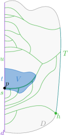
Figure 9: The part of $T$, the tree representing the Hamiltonian Voronoi diagram (green), that lies inside the Voronoi region $V$ (blue) of a new site $t$ is a subtree $T^{\prime}$ (fat). We can compute $T^{\prime}$, by exploring $T$ from a point $p$ inside $V$. In case $t$ is the first site in the ordering along $d$ we can start from the root $h$ of the “first” tree in $\mathcal{V}$.

Inserting a new site.

Klein and Lingas [15] sketch the following algorithm to insert a new site $t$ into the Hamiltonian Voronoi diagram $\mathcal{V}(S)$ of a set of sites $S$. We provide some missing details of this procedure, and briefly argue that we can use it to insert into a diagram of three sites. Let $D$ denote the domain in which we are interested in $\mathcal{V}(S)$ (in our application, $D$ is the subpolygon $P_{r}$) and let $d$ be the curve that intersects all regions in $\mathcal{V}(S)$. Recall that $\mathcal{V}(S)$ is a forest. We root all trees such that the leaves correspond to the intersections of the bisectors with $d$. The roots of the trees now corresponds to points along the boundary $\partial D$ of $D$. We connect them into one tree $T$ using curves along $\partial D$. Now consider the Voronoi region $V$ of $t$ with respect to $S\cup\{t\}$, and observe that $T\cap V$ is a subtree $T^{\prime}$ of $T$. Therefore, if we have a starting point $p$ on $T$ that is known to lie in $V$ (and thus in $T^{\prime}$), we can compute $T^{\prime}$ simply by exploring $T$. To obtain $\mathcal{V}(S\cup\{t\})$ we then simply remove $T^{\prime}$, and connect up the tree appropriately. See Fig. 9 for an illustration. We can test if a vertex $v$ of $T$ is part of $T^{\prime}$ simply by testing if $v$ lies on the $t$-side of the bisector between $t$ and one of the sites defining $v$. We can find the exact point $q$ where an edge $(u,v)$ of $T$, representing a piece of a bisector $b_{su}$ leaves $V$ by computing the intersection point of $b_{su}$ with $b_{tu}$ and $b_{st}$.

We can find the starting point $p$ by considering the order of the Voronoi regions along $d$. Let $s$ and $u$ be the predecessor and successor of $t$ in this order. Then the intersection point of $d$ with $b_{su}$ must lie in $V$. This point corresponds to a leaf in $T$. In case $t$ is the first site in the ordering along $d$ we start from the root $h$ of the tree that contains the bisector between the first two sites in the ordering; if this point is not on the $t$-side of the bisector between $t$ and one of the sites defining $h$ then $b_{tu}$ forms its own tree (which we then connect to the global root). We do the same when $t$ is the last point in the ordering. This procedure requires $O(|T^{\prime}|)$ time in total (excluding the time it takes to find $t$ in the ordering of $S$; we already have this information when the procedure is used in the algorithm of Klein and Lingas [15]).

We use the above procedure to compute the Voronoi diagram of five sites in constant time: simply pick three of the sites $s$, $t$, and $u$, ordered along $d$, compute their Voronoi diagram by computing the intersection of $b_{st}$ and $b_{tu}$ (if it exists), and insert the remaining two sites. Since the intermediate Voronoi diagrams have constant size, this takes constant time.

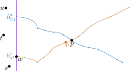
Figure 10: We find the intersection point of the two bisectors by binary searching along $b^{*}_{st}$.

Computing the intersection of bisectors $b^{*}_{st}$ and $b^{*}_{tu}$.

Since $\mathcal{V}$ is a Hamiltonian Voronoi diagram, any any pair of bisectors $b^{*}_{st}$ and $b^{*}_{tu}$, with $s,t,u\in T^{*}$, intersect at most once (Observation 19). Next, we show how to compute this intersection point (if it exists).

Lemma 20.

Given $\hat{\mathcal{P}}(z,s,t)$ and $\hat{\mathcal{P}}(z^{\prime},t,u)$, we can find the intersection point $p$ of $b^{*}_{st}$ and $b^{*}_{tu}$ (if it exists) in $O(\log^{2}m)$ time.

Proof. We will find the edge of $b^{*}_{st}$ containing the intersection point $p$ by binary searching along the vertices of $b^{*}_{st}$. Analogously we find the edge of $b^{*}_{tu}$ containing $p$. It is then easy to compute the exact location of $p$ in constant time.

Let $w$ be the starting point of $b^{*}_{st}$, i.e. the intersection of $b_{st}$ with $d$, and assume that $t$ is closer to $w$ than $u$, that is, $\scaleobj{1.7}{\varsigma}(t,w)<\scaleobj{1.7}{\varsigma}(u,w)$ (the other case is symmetric). In our binary search, we now simply find the last vertex $v=v_{k}$ for which $\scaleobj{1.7}{\varsigma}(t,v)<\scaleobj{1.7}{\varsigma}(u,v)$. It then follows that $p$ lies on the edge $(v_{k},v_{k+1})$ of $b^{*}_{st}$. See Fig. 10. Using Lemma 13 we can access any vertex of $b^{*}_{st}$ in $O(\log m)$ time. Thus, this procedure takes $O(\log^{2}m)$ time in total. ∎

Note that we can easily extend the algorithm from Lemma 20 to also return the actual edges of $b^{*}_{st}$ and $b^{*}_{tu}$ that intersect. With this information we can construct the cyclic order of the edges incident to the vertex of $\mathcal{V}$ representing this intersection point. It now follows that for every group $S^{*}$ of sites in $P_{\ell}$, we can compute a representation of $\mathcal{V}$ of size $O(k)$ in $O(k\log^{2}m)$ time.

4.3 Planar Point Location in $\mathcal{V}$

In this section we show that we can efficiently answer point location queries, and thus nearest neighbor queries using $\mathcal{V}$.

Lemma 21.

For $s,t\in S_{\ell}$, the part of the bisector $b^{*}_{st}=b_{st}\cap P_{r}$ that lies in $P_{r}$ is $x$-monotone.

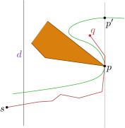
Figure 11: A non $x$-monotone bisector can occur only in degenerate inputs.

Proof. Assume, by contradiction, that $b_{st}$ is not $x$-monotone in $P_{r}$, and let $p$ be a point on $b_{st}$ such that $p_{x}$ is a local maximum. Since $b^{*}_{st}$ is not $x$-monotone, it intersects the vertical line through $p$ also in another point $p^{\prime}$ further along $b^{*}_{st}$. Let $q$ be a point in the region enclosed by the subcurve along $b^{*}_{st}$ from $p$ to $p^{\prime}$ and $\overline{pp^{\prime}}$. See Fig. 11. This means that either $\scaleobj{1.15}{\varsigma}(s,q)$ or $\scaleobj{1.15}{\varsigma}(t,q)$ is non $x$-monotone. Assume without loss of generality that it is $\scaleobj{1.15}{\varsigma}(s,q)$. It is now easy to show that $\scaleobj{1.15}{\varsigma}(s,q)$ must pass through $p$. However, that means that $b^{*}_{st}$ (and thus $b_{st}$) touches the polygon boundary in $p$. By the general position assumption $b_{st}$ has no points in common with $\partial P$ other than its end points. Contradiction. ∎

Since the (restriction of the) bisectors are $x$-monotone (Lemma 21) we can preprocess $\mathcal{V}$ for point location using the data structure of Edelsbrunner and Stolfi [8]. Given the combinatorial embedding of $\mathcal{V}$, this takes $O(|\mathcal{V}|)$ time. To decide if a query point $q$ lies above or below an edge $e\in\mathcal{V}$ we simply compute the distances $\scaleobj{1.7}{\varsigma}(s,q)$ and $\scaleobj{1.7}{\varsigma}(t,q)$ between $q$ and the sites $s$ and $t$ defining the bisector corresponding to edge $e$. This takes $O(\log m)$ time. Point $q$ lies on the side of the site that has the shorter distance. It follows that we can preprocess $\mathcal{V}$ in $O(k)$ time, and locate the Voronoi region containing a query point $q$ in $O(\log k\log m)$ time. We summarize our results in the following Lemma.

Lemma 22.

Given a set of $k$ sites $S^{*}$ in $P_{\ell}$, ordered by increasing distance from the bottom-endpoint of $d$, we can construct the forest $\mathcal{V}$ representing the Voronoi diagram of $S^{*}$ in $P_{r}$ in $O(k\log^{2}m)$ time. Given $\mathcal{V}$, we can find the site $s\in S^{*}$ closest to a query point $q\in P_{r}$ in $O(\log k\log m)$ time.

5 Putting Everything Together

For every level of the balanced decomposition, we split $S_{\ell}$ into $O(\sqrt{n})$ groups, and for each group build the Voronoi diagram in $P_{r}$ using the approach from Section 4. We process the sites in $S_{r}$ analogously. This leads to the following result.

Theorem 23.

Given a polygon $P$ with $m$ vertices, we can build a fully dynamic data structure of size $O(n\log m+m)$ that maintains a set of $n$ point sites in $P$ and allows for geodesic nearest neighbor queries in $O(\sqrt{n}\log n\log^{2}m)$ time. Inserting or deleting a site takes $O(\sqrt{n}\log^{3}m)$ time.

Proof.

Since every site occurs in exactly one group per level of the balanced decomposition, and there are $O(\log m)$ levels, the total space required for our data structure is $O(n\log m+m)$. Similarly, when we insert or delete a site, we have to insert or delete it in $O(\log m)$ levels. Each such insertion or deletion takes $O(\sqrt{n}\log^{2}m)$ time, as we have to rebuild a Voronoi diagram for one group. For a query, we have to query all $O(\sqrt{n})$ groups in $O(\log m)$ levels. This leads to a total query time of $O(\sqrt{n}\log n\log^{2}m)$. ∎

Insertions only.

In case our data structure has to support only insertions, we can improve the insertion time to $O(\log n\log^{3}m)$, albeit being amortized. Recall that at every node of the balanced decomposition our data structure partitions the sites in $S_{\ell}$ in $O(\sqrt{n})$ groups of size $O(\sqrt{n})$ each. Instead, we now maintain these sites in groups of size $2^{i}$, for $i\in[1..O(\log n)]$. When we insert a new site, we may get two groups of size $2^{i}$. We then remove these groups, and construct a new group of size $2^{i+1}$. For this group we rebuild the Voronoi diagram $\mathcal{V}$ that these sites induce on $P_{r}$ from scratch. Using a standard binary counter argument it can be shown that every data structure of size $2^{i+1}$ gets rebuild (at a cost of $O(2^{i}\log^{2}m)$) only after $2^{i}$ new sites have been inserted [19]. So, if we charge $O(\log n\log^{2}m)$ to each site, it can pay for rebuilding all of the structures it participates in. We do this for all $O(\log m)$ levels in the balanced decomposition, hence we obtain the following result.

Corollary 24.

Given a polygon $P$ with $m$ vertices, we can build an insertion-only data structure of size $O(n\log m+m)$ that stores a set of $n$ point sites in $P$, and allows for geodesic nearest neighbor queries in worst-case $O(\log^{2}n\log^{2}m)$ time, and allows inserting a site in amortized $O(\log n\log^{3}m)$ time.

Offline updates.

When we have both insertions and deletions, but the order of these operations is known in advance, we can maintain $S$ in amortized $O(\log n\log^{3}m)$ time per update, where $n$ is the maximum number of sites in $S$ at any particular time. Queries take $O(\log^{2}n\log^{2}m)$ time, and may arbitrarily interleave with the updates. Furthermore, we do not have to know them in advance.

For ease of description, we assume that the total number of updates $N$ is proportional to the number of sites at any particular time, i.e. $N\in O(n)$. We can easily extend our approach to larger $N$ by grouping the updates in $N/n$ groups of size $O(n)$ each. Consider a node of the balanced decomposition whose diagonal that splits its subpolygon into $P_{\ell}$ and $P_{r}$. We partition the sites in $S_{\ell}$ into groups such that at any time, a query $q\in P_{r}$ can be answered by considering the Voronoi diagrams in $P_{r}$ of only $O(\log n)$ groups. We achieve this by building a segment tree on the intervals during which the sites are “alive”. More specifically, let $[t_{1},t_{2}]$ denote a time interval in which a site $s$ should occur in $S_{\ell}$ (i.e. $s$ lies in $P_{\ell}$ and there is an Insert($s$) operation at time $t_{1}$ and its corresponding Delete($s$) at time $t_{2}$). We store the intervals of all sites in $S_{\ell}$ in a segment tree [6]. Each node $v$ in this tree is associated with a subset $S_{v}$ of the sites from $S_{\ell}$. We build the Voronoi diagram that $S_{v}$ induces on $P_{r}$. Every site occurs in $O(\log n)$ subsets, and in $O(\log m)$ levels of the balanced decomposition, so the total size of our data structure is $O(n\log n\log m+m)$. Building the Voronoi diagram for each node $v$ takes $O(|S_{v}|\log^{2}m)$ time. Summing these results over all nodes in the tree, and all levels of the balanced decomposition, the total construction time is $O(n\log n\log^{3}m+m)$ time. We conclude:

Corollary 25.

Given a polygon $P$ with $m$ vertices, and a sequence of operations that either insert a point site inside $P$ into a set $S$, or delete a site from $S$, we can maintain a dynamic data structure of size $O(n\log n\log m+m)$, where $n$ is the maximum number of sites in $S$ at any time, that stores $S$, and allows for geodesic nearest neighbor queries in $O(\log^{2}n\log^{2}m)$ time. Updates take amortized $O(\log n\log^{3}m)$ time.

References

- [1] P. K. Agarwal and J. Matoušek. Dynamic Half-Space Range Reporting and its Applications. Algorithmica, 13(4):325–345, 1995.
- [2] B. Aronov. On the Geodesic Voronoi Diagram of Point Sites in a Simple Polygon. Algorithmica, 4(1):109–140, 1989.
- [3] J. L. Bentley and J. B. Saxe. Decomposable searching problems I. Static-to-dynamic transformation. Journal of Algorithms, 1(4):301–358, 1980.
- [4] M. T. Burrows, D. S. Schoeman, A. J. Richardson, J. G. Molinos, A. Hoffmann, L. B. Buckley, P. J. Moore, C. J. Brown, J. F. Bruno, C. M. Duarte, et al. Geographical limits to species-range shifts are suggested by climate velocity. Nature, 507(7493):492–495, 2014.
- [5] T. M. Chan. A Dynamic Data Structure for 3-D Convex Hulls and 2-D Nearest Neighbor Queries. J. ACM, 57(3):16:1–16:15, Mar. 2010.
- [6] M. de Berg, O. Cheong, M. van Kreveld, and M. Overmars. Computational Geometry: Algorithms and Applications. Springer, 3rd edition, 2008.
- [7] D. Dobkin and S. Suri. Maintenance of Geometric Extrema. J. ACM, 38(2):275–298, Apr. 1991.
- [8] H. Edelsbrunner, L. Guibas, and J. Stolfi. Optimal Point Location in a Monotone Subdivision. SIAM Journal on Computing, 15(2):317–340, May 1986.
- [9] L. Guibas, J. Hershberger, D. Leven, M. Sharir, and R. E. Tarjan. Linear-Time Algorithms for Visibility and Shortest Path Problems Inside Triangulated Simple Polygons. Algorithmica, 2(1):209–233, 1987.
- [10] L. J. Guibas and J. Hershberger. Optimal Shortest Path Queries in a Simple Polygon. Journal of Computer and System Sciences, 39(2):126 – 152, 1989.
- [11] J. Hershberger. A new data structure for shortest path queries in a simple polygon. Information Processing Letters, 38(5):231–235, June 1991.
- [12] J. Hershberger and S. Suri. An Optimal Algorithm for Euclidean Shortest Paths in the Plane. SIAM J. Comput., 28(6):2215–2256, 1999.
- [13] H. Kaplan, W. Mulzer, L. Roditty, P. Seiferth, and M. Sharir. Dynamic Planar Voronoi Diagrams for General Distance Functions and their Algorithmic Applications. In Proc. 28th Annual ACM-SIAM Symposium on Discrete Algorithms. SIAM, 2017.
- [14] R. Klein. Concrete and abstract Voronoi diagrams, volume 400. Springer Science & Business Media, 1989.
- [15] R. Klein and A. Lingas. Hamiltonian abstract Voronoi diagrams in linear time, pages 11–19. Springer Berlin Heidelberg, Berlin, Heidelberg, 1994.
- [16] R. Klein, K. Mehlhorn, and S. Meiser. Randomized incremental construction of abstract Voronoi diagrams. Computational Geometry, 3(3):157 – 184, 1993.
- [17] E. Oh and H.-K. Ahn. Voronoi Diagrams for a Moderate-Sized Point-Set in a Simple Polygon. In B. Aronov and M. J. Katz, editors, 33rd International Symposium on Computational Geometry (SoCG 2017), volume 77 of Leibniz International Proceedings in Informatics (LIPIcs), pages 52:1–52:15, Dagstuhl, Germany, 2017. Schloss Dagstuhl–Leibniz-Zentrum fuer Informatik.
- [18] A. Ordonez and J. W. Williams. Climatic and biotic velocities for woody taxa distributions over the last 16 000 years in eastern north america. Ecology letters, 16(6):773–781, 2013.
- [19] M. H. Overmars. The design of dynamic data structures, volume 156. Springer Science & Business Media, 1983.
- [20] E. Papadopoulou and T. D. Lee. A New Approach for the Geodesic Voronoi Diagram of Points in a Simple Polygon and Other Restricted Polygonal Domains. Algorithmica, 20(4):319–352, 1998.