Mirror symmetry for very affine hypersurfaces

Abstract.

We show that the category of coherent sheaves on the toric boundary divisor of a smooth quasiprojective toric DM stack is equivalent to the wrapped Fukaya category of a hypersurface in $(\mathbb{C}^{\times})^{n}$. Hypersurfaces with every Newton polytope can be obtained.

Our proof has the following ingredients. Using recent results on localization, we may trade wrapped Fukaya categories for microlocal sheaf theory along the skeleton of the hypersurface. Using Mikhalkin-Viro patchworking, we identify the skeleton of the hypersurface with the boundary of the Fang-Liu-Treumann-Zaslow skeleton. By proving a new functoriality result for Bondal’s coherent-constructible correspondence, we reduce the sheaf calculation to Kuwagaki’s recent theorem on mirror symmetry for toric varieties.

1. Introduction

Homological mirror symmetry is a story of two categories radically different in origin. The first is a category of Lagrangians in a symplectic manifold, with morphisms defined by intersection points, corrected by holomorphic disks. The second is a category of locally defined modules over the holomorphic functions on a seemingly unrelated complex variety, with morphisms corrected by considerations of homological algebra. Most articles on the subject concern the ingenious manipulations required to identify one with the other, most often requiring heroic calculations of at least one side of this equivalence.

Our contribution is of a different nature. We wish to explain how in many circumstances – we focus on Calabi-Yau hypersurfaces in toric varieties, though the same methods should apply in the generality of Gross-Siebert toric degenerations – both sides can be cut into matching elementary pieces, known to be homologically mirror, and the total mirror symmetry glued together using foundational results in algebraic and symplectic geometry. More precisely, this cutting and gluing is possible at the limiting point where on the one hand the complex manifold degenerates into a union of toric varieties, while on the other, the symplectic form concentrates along certain divisors, and we consider the category associated to their complement. We will be entirely concerned with homological mirror symmetry at this limit point.

At this most degenerate point, the category of coherent sheaves on the union of toric varieties – glued together along toric subvarieties – can be calculated as a colimit of the categories of coherent sheaves on the toric components [GR].

Mirror symmetry is well studied for toric varieties themselves. The Hori-Vafa prescription is that the mirror A-model category should be associated to a function $W:(\mathbb{C}^{*})^{n}\to\mathbb{C}$ whose Newton polytope is the convex hull of primitive vectors on the 1-dimensional cones of the fan of the toric variety. Different authors have taken different views on how precisely to associate a category to this geometry, either directly in Lagrangian Floer theory [A1, A2], or in microlocal sheaf theory [B, FLTZ, Tr, Ku] (the latter being known to be calculate Fukaya categories [NZ, N1, GPS3]).

A true believer in mirror symmetry should expect the following facts:

1. The mirror to the toric boundary – a generic fiber of a generic $W:(\mathbb{C}^{*})^{n}\to\mathbb{C}$ whose Newton polytope is the moment polytope of the toric variety – admits a cover by mirrors of toric varieties, glued along mirrors of toric varieties.

2. There are geometrically defined functors between these Fukaya categories which are mirror to the pullback and pushforward functors corresponding to the inclusion of toric varieties in toric varieties.

3. There is a descent result for the Fukaya category showing that it carries covers of the sort in (1) to colimits of categories.

Establishing all of these results would show that the Fukaya category of the general fiber of $W$ is equivalent to the category of coherent sheaves of the corresponding toric variety. The recent works [GPS1, GPS2, GPS3] give the necessary general tools to define the functors in (2) and establish the descent required in (1). In fact, these works, together with [NS], build a bridge between Fukaya categories and microlocal sheaf theory, which we cross in order to appeal to the microlocal sheaf calculations of the toric mirror [Ku]. Here we will establish (1) and the ‘mirror’ assertions of (2) above, and deduce:

Theorem 1.0.1.

Suppose we are given the following data:

• $\mathbb{T}_{\mathbb{C}}$ an algebraic torus with character and cocharacter lattices $M$ and $M^{\vee}$.

• $\Delta^{\vee}\subset M^{\vee}$ an integral polytope containing the origin.

• $\Sigma$ a fan in $M^{\vee}\otimes\mathbb{R}$ giving a star-shaped triangulation of $\Delta^{\vee}$.

These determine a smooth toric stack $\mathbf{T}_{\Sigma}$ with toric boundary divisor $\partial\mathbf{T}_{\Sigma}$.

Then there exists a Laurent polynomial $W:\mathbb{T}^{\vee}_{\mathbb{C}}\to\mathbb{C}$ with Newton polytope $\Delta^{\vee}$; a natural structure of Liouville manifold on a general fiber $F_{W}$; and an equivalence

$$\textup{Coh}(\partial\mathbf{T}_{\Sigma})\cong\textup{Fuk}(F_{W})$$

between the dg category of coherent sheaves on the variety $\partial\mathbf{T}_{\Sigma}$ and the wrapped Fukaya category of the general fiber $F_{W}$

We close the introduction with some comments about how we will establish items (1) and (2) above.

Regarding (1): in the microlocal sheaf theoretic works beginning with [FLTZ], a key role is played by a certain conical Lagrangian subvariety $\Lambda_{\Sigma}\subset T^{*}\mathbb{T}\cong\mathbb{T}^{\vee}_{\mathbb{C}}$. It is straightforward to establish that the boundary of this conical subvariety indeed admits a cover corresponding to the cover of the $\partial\mathbf{T}$ by toric subvarieties. What is needed is to relate the geometry of $\Lambda_{\Sigma}$ to the geometry of the Laurent polynomial $W$. One result along these lines which we shall establish is that the deformation equivalence class of the Liouville sector determined by $W$ admits a representative whose relative skeleton is precisely $\Lambda_{\Sigma}$. Another is that a neighborhood of the boundary of this sector admits a sectorial cover by sectors whose relative skeleta give the aforementioned cover of $\Lambda_{\Sigma}$. These results are established in Section 6 by using the Mikhalkin-Viro patchworking to reduce the study of $F_{W}$ to understanding pairs of pants, whose skeleta have been calculated by Nadler.

Regarding (2): after the geometric results in the previous paragraph, existence of the relevant functors of Fukaya categories can be deduced from [GPS1]. To calculate them, we use [GPS3, NS] to pass to microlocal sheaf theory, where we must now show that the mirror symmetry established in [Ku] can be made functorial with respect to inclusion of toric boundary divisors. We explain how to do this in Section 7.

In the following section, we explain in more detail the general strategy of the proof, reviewing relevant ideas from sources mentioned above, and we give the proof of Theorem 1.0.1, up to the calculations mentioned in the previous two paragraphs, which we defer to the main body of the paper.

Acknowledgements — We thank Sheel Ganatra, Stephane Guillermou, Allen Knutson, Tatsuki Kuwagaki, Heather Lee, Grigory Mikhalkin, David Nadler, Martin Olsson, John Pardon, Pierre Schapira, Nick Sheridan, Laura Starkston, and Zack Sylvan for helpful conversations on various related topics. The authors are also thankful to Peng Zhou for notifying us of an omission in an earlier version of this paper.

The work of B.G. was supported by an NSF Graduate Research Fellowship, and V.S. was supported by NSF DMS-1406871, NSF CAREER DMS-1654545, and a Sloan fellowship.

2. Our approach to homological mirror symmetry

2.1. An illustration

Consider the degeneration in which a genus-one holomorphic curve acquires a node. In the mirror degeneration, a symplectic 2-torus acquires a puncture.

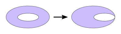
Figure 1. The degeneration of a smooth genus-one curve to a nodal curve.

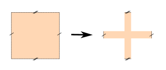
Figure 2. A torus acquiring a puncture as an $S^{1}$ fiber approaches infinite radius.

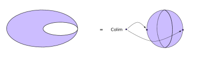
Figure 3. We obtain a nodal curve by gluing smooth pieces.

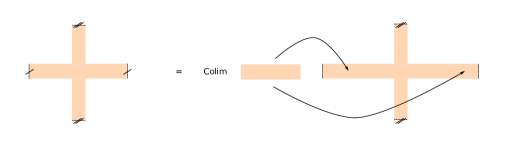
Figure 4. The mirror to the above gluing: a punctured torus is glued together from Liouville sectors.

One way to arrive at the view that these two spaces should be mirror is the following “T-duality” account. In general, the spaces on the two sides of mirror symmetry are expected to be dual torus fibrations (in general, with singularities) over the same base, the radii of the fibers on one side being inverse to the radii on the other side. In the present example, on the complex side, we have a torus – a circle bundle over a circle. Under the degeneration, one of the circle fibers is approaching zero radius. Thus, on the symplectic side, we should have a circle bundle over a circle, in which one fiber is approaching infinite radius. A circle of infinite radius is a line – or in other words, the fiber should acquire a puncture.

In the description above, the puncture was just the removal of a point. As we draw only the complement of this point, we are free to imagine the puncture as being larger, as in Figure 2. In our previous description, the fiber containing the puncture was dual to the node. We have expanded the puncture, so in this picture, one should regard the entire horizontal region beneath the puncture as being dual to the node.

On the complex side, we have a singular complex curve; it is natural to take the normalization. This is a smooth curve mapping to the singular curve, and in the case at hand, the map simply identifies points. This is what is indicated in Figure 3. We can describe the symplectic side by a similar gluing. Since the node corresponded to the strip beneath the puncture, the mirror gluing on the A-side involves gluing the two ends of the strip.

The category we associate to this noncompact symplectic manifold is the wrapped Fukaya category, which was originally constructed for Liouville manifolds, symplectic manifolds with the property that (at least locally near the boundary) there is a primitive for the symplectic form whose dual Liouville vector field is everywhere outward pointing [AS]. In the above gluing, however, the restriction of this Liouville form to the components does not have this property: there are boundary components where it is parallel, rather than outward pointing. In particular, the rectangle should be viewed as the cotangent bundle of an interval rather than a disk. That is, the pieces in our gluing are not Liouville manifolds. The appropriate notion is that of Liouville sector, which we review in the next subsection. A covariantly functorial Floer theory for these is developed in [GPS1, GPS2].

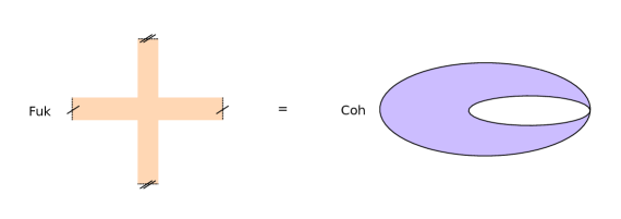
Figure 5. The homological mirror symmetry conjecture for a genus-one curve at the large volume/complex structure limits.

We turn now to the question of gluing together a global mirror symmetry from local mirror symmetries. The functor $\textup{Coh}(-)$ taking a variety $X$ to its dg category $\textup{Coh}(X)$ of coherent sheaves behaves well with respect to the gluings above. Following [GR], we make statements for the Ind-completion $\textup{IndCoh}(X)$ of the category $\textup{Coh}(X)$; statements for $\textup{Coh}(X)$ may be recovered by taking compact objects. We write $\textup{IndCoh}^{!}$ and $\textup{IndCoh}_{*}$ for the contravariant and covariant functors from derived stacks to dg categories which carry a stack to its category of Ind-coherent sheaves and carry a map $f:X\to Y$ to a pullback $f^{!}$ or a pushforward $f_{*}$, respectively. The key fact [GR, IV.4.A.1.2] is that $\textup{IndCoh}^{!}$ takes pushout squares of affine schemes along closed embeddings to pullback squares of (stable cocomplete) dg categories. By passing to adjoints, we see that $\textup{IndCoh}_{*}$ analogously takes pushouts to pushouts.

Homological mirror symmetry as usually stated is an equivalence between coherent sheaves on a given algebraic variety and the Fukaya category of its mirror. What the pictures above suggest is that this should extend to a natural transformation between the functor $\textup{IndCoh}_{*}$, perhaps with respect to some restricted class of maps including normalizations, and a functor $\textup{IndFuk}_{*}$, covariant with respect to some class of maps including those mirror to normalization. It suggests moreover that $\textup{IndFuk}_{*}$ should take certain diagrams – those mirror to certain pushouts of varieties – to pushouts of dg or $A_{\infty}$ categories.

In fact, a covariant functor from a category of Liouville sectors to $A_{\infty}$ categories has been defined in [GPS1], and shown in [GPS2] to carry diagrams like those illustrated above to pushouts. Given these structural properties, one can establish mirror symmetry by showing that there is an identification, respecting the relevant inclusion functors, of the Fukaya and coherent-sheaf categories of our building blocks.

Remark 2.1.1.

Strictly speaking, this subsection does not illustrate a special case of the statement of Theorem 1.0.1, because the self-nodal curve is not the boundary of a toric variety. However, an essentially identical argument gives the mirror symmetry between the nodal necklace of three $\mathbb{P}^{1}$s and a thrice-punctured torus, which is a special case of Theorem 1.0.1.

This subsection also does not exactly illustrate the proof we will give of Theorem 1.0.1; instead, as we explain below, we will translate these ideas to the microlocal sheaf setting using [GPS3]. In this setting, we need only cover the skeleton, as we do in Corollary 4.3.2. A lift of this cover to a sectorial cover in the sense of [GPS2] would yield a proof hewing closer to the above illustration.

2.2. Stops, sectors, skeleta, and partially wrapped Fukaya categories.

For basics on Liouville and Weinstein manifolds, we refer to [CE, Eli]. Here we review basic notions of Liouville sectors, stops, and skeleta, and then recall from [GPS1, GPS2] definitions and results concerning partially wrapped Fukaya categories defined in terms of these geometric structures.

A Liouville sector is an exact symplectic manifold-with-boundary $(X,\partial X,\lambda)$ modeled at infinity on the symplectization of a contact manifold-with-boundary $(V,\partial V,\lambda)$, satisfying additional constraints: $\partial V$ should be transverse to a contact vector field, and the characteristic foliation on $\partial X$ should be trivializable as $\partial X=\mathbb{R}\times F$. Such a trivialization makes $(F,\lambda|_{F})$ a Liouville manifold. Note that being a Liouville sector is a property of, rather than a structure on, an exact symplectic manifold-with-boundary.

A closed codimension zero submanifold-with-boundary $Y\subset X$ is a Liouville subsector if (1) each component of $\partial Y$ is either disjoint from or contained in $\partial X$, and (2) $(Y,\partial Y,\lambda|_{\partial Y})$ is itself a Liouville sector. One can see by inspection that the symplectic manifolds in Figure 4 admit an exact structure making them Liouville sectors, and that the inclusions depicted are inclusions of Liouville sectors.

Another point of view on sectors is obtained by passing to the ‘convex completion’ $\bar{X}$, which is a Liouville manifold in the usual sense. Up to contractible choices, the data of the sector is equivalent to an embedding $F\subset\partial_{\infty}\bar{X}$ as a Liouville hypersurface, i.e. some choice of contact form on $\partial_{\infty}\bar{X}$ restricts to the Liouville form on $F$. The $(\bar{X},F)$ form what is termed a Liouville pair elsewhere in the literature [Avd, Syl, Eli]. The advantage of Liouville sectors over Liouville pairs is that they are better suited to discussions of gluing, in particular because the key notion of Liouville subsector is less natural in the setting of pairs. Basic definitions and constructions relevant to Liouville sectors are found in [GPS1, Sec. 2].

We refer to works [AS, GPS1, GPS2] for a foundational treatment of partially wrapped Fukaya categories. For our purposes here, we may largely use these works as black boxes. The most general setting for defining partially wrapped Fukaya categories (offered by [GPS2]) takes as input the data of a Liouville sector $X$ and a closed subset in the infinite boundary $\Lambda\subset\partial_{\infty}X^{\circ}$. (We recall that a Liouville sector has its actual boundary $\partial X$, and its ideal contact boundary $\partial_{\infty}X$; here $\partial^{\infty}X^{\circ}$ means the contact boundary minus its intersection with the actual boundary $\partial X$.) To such a pair is associated a category which we here denote $Fuk(X,\Lambda)$.

A stopped sector includes in another by enlarging the sector or shrinking the stop: we say $(X^{\prime},\Lambda^{\prime})\subset(X,\Lambda)$ if $X^{\prime}$ is a Liouville subsector of $X$ and $\Lambda^{\prime}\supset\Lambda\cap X^{\prime}$. It is shown in [GPS1, GPS2] that in this case there is a functor

$$Fuk(X^{\prime},\Lambda^{\prime})\to Fuk(X,\Lambda)$$

When $X=X^{\prime}$ we term this functor a “stop removal.” These satisfy the natural compatibilities with composition, defining a (strict!) functor from the poset of (stopped) subsectors of $(X,\Lambda)$ to $A_{\infty}$ categories.

To a Liouville manifold $X$ is associated the skeleton (elsewhere termed spine or core) $\mathfrak{c}_{X}$, this being the locus of all points which do not escape to infinity under the Liouville flow. When the Liouville flow is gradient-like and generalized Morse-Smale (such manifolds are said to be Weinstein), the skeleton is admits a Whitney stratification by isotropic submanifolds, and the top-dimensional strata admit transverse “cocore” Lagrangian disks. It is this consequence which is relevant for [GPS2, GPS3], and some weaker definitions of Weinstein have been proposed which imply it; see for instance [Eli]. The above results remain true when the Liouville flow is Morse-Bott, as in the cases studied in this paper.

For a Liouville sector $X$, one can define the skeleton $\mathfrak{c}_{X}$ by the same formulation: $\mathfrak{c}_{X}$ is the locus which does not escape to infinity. However, this definition is only really sensible if the Liouville flow on $X$ is tangent to $\partial X$ along all of $\partial X$, not just at the boundary. Note [GPS1, Lemma 2.11, Prop 2.28] this can always be arranged after deformation. Evidently, if $X\subset Y$ is an inclusion of Liouville sectors where $\lambda_{X}=\lambda_{Y}|_{X}$ and the Liouville flow on $X$ is tangent to its boundary, then $\mathfrak{c}_{X}=\mathfrak{c}_{Y}\cap X$.

We offer also another perspective on the skeleton of a sector. Recall that a sector $X$ is equivalent to the data of a pair $(\bar{X},F\subset\partial_{\infty}\bar{X})$. For the pair, it is natural to define the relative skeleton $\mathfrak{c}_{\bar{X},F}$ as the locus of points $\bar{X}$ which do not escape to $\partial_{\infty}\bar{X}\setminus\mathfrak{c}_{F}$. Note that this is the union of $\mathfrak{c}_{X}$ with a $\mathbb{R}$-cone on $\mathfrak{c}_{F}$. This notion of relative skeleton compares to the skeleton of a sector as follows: it is not difficult, using the techniques of [GPS1, Sec. 2] to arrange an inclusion of sectors $X\subset\bar{X}$ such that $\mathfrak{c}_{X}=\mathfrak{c}_{\bar{X},F}\cap X$.

From the point of view of Fukaya categories, the significance of skeleta and relative skeleta is in their role in organizing generation results. Indeed, the cocore disks to a Weinstein Morse function provide Lagrangians transverse to each component of the smooth locus of the skeleton, and at any Legendrian point of a stop there is associated a linking disk; according to [GPS2, Thm. 1.10], these generate $Fuk(X,\Lambda)$ when $X$ is a Weinstein manifold and $\Lambda$ is mostly Legendrian.

For calculating Fukaya categories, we may always translate back and forth between Liouville sectors and stopped Liouville manifolds, and further we may retract the stop to its skeleton. Indeed, per [GPS2, Cor. 2.11], we have equivalences

$$Fuk(X)\xrightarrow{\sim}Fuk(\bar{X},F)\xrightarrow{\sim}Fuk(\bar{X},\mathfrak{c}_{F}).$$

2.3. LG model

Partially wrapped Fukaya categories can be used to formulate homological mirror symmetry for Fano varieties. For example, the mirror to $\mathbb{P}^{1}$ should be somehow associated to the function $W(z)=z+z^{-1}$ on $\mathbb{C}^{*}$. We interpret this to mean that we should form a Liouville sector from $\mathbb{C}^{*}$ by deleting the neighborhood of a fiber $W^{-1}(-\infty)$ at infinity. In this special case, any reasonable interpretation of the above description should result in the sector on the left-hand side of Figure 5.

More generally, we would like to obtain a Liouville sector from a function $W:(\mathbb{C}^{*})^{n}\to\mathbb{C}$, as such functions were predicted by Hori and Vafa [HV] to provide mirrors to toric varieties. Naïvely, one could attempt to produce a sector from this data as follows: take a half-plane $\mathbb{H}\subset\mathbb{C}$ containing all the critical values (including those associated to critical points at infinity) of $W$, and take $W^{-1}(\mathbb{H})$ as the sector. Strictly speaking, however, $W^{-1}(\mathbb{H})$ is not generally conical at infinity for the restriction of the most natural Liouville structure on $(\mathbb{C}^{*})^{n}$, so some manipulation of exact structures and use of cutoff functions would be necessary. Similar issues arise in work of Seidel, see e.g. [Sei3, Sec. 3A] and [Sei2, Sec. 19B]. Instead, we use the tropical methods of [M, A1] to show the following:

Proposition 2.3.1.

Fix a Newton polytope $\Delta^{\vee}\subset\mathbb{Z}^{n}$ and regular star subdivision $\mathcal{T}$ induced by some piecewise-linear function $\alpha$. Consider the Laurent polynomial

$$W(z)=\sum_{m\in V}t^{-\alpha(m)}z^{m}.$$

There is a real codimension-2 symplectic submanifold $F_{\Sigma}$ of $(\mathbb{C}^{*})^{n}$ such that:

• [A1] For $t\gg 0$, there is an isotopy of symplectic submanifolds between $F_{\Sigma}$ and a general fiber $F_{W}$ of $W$.

• There is a Liouville subdomain $D\subset(\mathbb{C}^{*})^{n}$, completing to $(\mathbb{C}^{*})^{n}$, such that $\partial D\cap F_{\Sigma}$ is a Liouville subdomain of $F_{\Sigma}$, completing to $F_{\Sigma}$.

As indicated, the first item is proven in [A1], in a form we recall in Lemma 6.1.6. The second item follows from our further calculations that that the skeleton of $F_{\Sigma}$ is contained in the boundary of some subdomain $D$ (Theorem 6.2.4), and moreover, along the skeleton, $F_{\Sigma}$ is nowhere tangent to the Liouville vector field of the ambient $(\mathbb{C}^{*})^{n}$ (Lemma 6.2.5). Indeed, then we may deform slightly $\partial D$ along the Liouville field in order to contain some neighborhood of the skeleton of $F_{\Sigma}$.

It is the sector associated to the particular pair $(D,F_{\Sigma}\cap D)$ constructed by our proof of this proposition that is used in this article. In particular in Theorem 1.0.1, when we assert ‘there is a Liouville structure on $F_{W}$’ we mean that we pull back the Liouville structure mentioned above under the symplectomorphism $F_{W}\cong F_{\Sigma}$.

Of course, we expect that any other reasonable construction of such a pair from $W$ will be deformation equivalent to ours, in particular giving the same Fukaya category.

2.4. Sheaves

A prototypical example of a Liouville manifold is the cotangent bundle $T^{*}M$ of a closed manifold without boundary; the skeleton for the usual “$pdq$” form is the zero section. If $M$ had boundary, the cotangent bundle would naturally be a Liouville sector, again with the zero section as skeleton. An open set $U\subset M$ determines an inclusion of Liouville sectors $T^{*}U\subset T^{*}M$: the stopped boundary of $T^{*}U$ is the restriction of the cotangent bundle to the boundary of $U$. Lifting a cover of $M$ gives a cover of $T^{*}M$ by Liouville sectors, whose intersections are again Liouville sectors (with corners). The covariantly functorial [GPS1] assignment $U\mapsto Fuk(T^{*}U)$ thus defines a precosheaf of categories on $M$.

Suppose we knew this precosheaf were a cosheaf. Then we could compute its global sections from the local data. Indeed, the Fukaya category of the cotangent bundle of a disk is equivalent to the category of chain complexes, so the cosheaf in question would be a locally constant cosheaf of categories. Recall that the $\infty$-groupoidal version of the Seifert-van Kampen theorem asserts that the fundamental higher groupoid of a space is the global sections of a locally constant cosheaf of spaces with stalk a point. Linearizing this, we see that a locally constant cosheaf of $A_{\infty}$ categories with stalk the category of chain complexes has global sections (a twisted version of) the category of modules over the algebra of chains on the based loop space of $M$. Thus, the Fukaya category of a cotangent bundle is the category of modules over chains on the based loop space. This final statement is originally a result of Abouzaid, by a different argument [A3].

Kontsevich’s localization conjecture [Kon2] asserts that the existence of a similar cosheaf $\mathcal{F}uk$ over the skeleton of any Weinstein manifold (e.g. the complement of an ample divisor in a smooth projective variety), whose global sections should recover the wrapped Fukaya category.

A variant, which gives a local-to-global principle without any mention of skeleta, is the main result of [GPS2], which asserts that the Fukaya category satisfies descent with respect to sectorial covers. This result, together with the well known calculation of Fukaya categories of disks with stops at the boundary (for a very short calculation, see [GPS2, Ex. 1.22]), can easily be used to make the discussion of Section 2.1 above completely rigorous.

In the body of this article we will need a further elaboration of Kontsevich’s conjecture, formulated by Nadler [N4] (and further elaborated in [S, NS]), which identifies Kontsevich’s conjectural cosheaf of categories on the skeleton with a certain cosheaf of a combinatorial-topological nature which is constructed directly from the microlocal sheaf theory of [KS]. This conjecture is established in [GPS3], using the theory developed in [GPS1, GPS2] and the antimicrolocalization lemma of [NS].

2.5. Proof of Theorem 1.0.1

Here we give the proof of Theorem 1.0.1, modulo the results which are the essential mathematical contents of the present article. We fix the following notations for the relevant toric data. (A brief review of relevant algebraic geometry of toric varieties is included in Section 3.)

Let $\mathbb{T}$ be a real $n$-dimensional torus. Let $M$ and $M^{\vee}$ be its lattices of characters and cocharacters, respectively. For an abelian group $A$, we write $M_{A}:=M\otimes_{\mathbb{Z}}A$. We can then write the torus $\mathbb{T}$ and its dual as

We denote the corresponding complex tori by $\mathbb{T}_{\mathbb{C}}=M^{\vee}_{\mathbb{C}^{\times}},$ $\mathbb{T}_{\mathbb{C}}^{\vee}=M_{\mathbb{C}^{\times}}.$

These complex tori are naturally tangent bundles, $\mathbb{T}_{\mathbb{C}}^{\vee}\cong T\mathbb{T}^{\vee}=(M_{\mathbb{R}}/M)\times M_{\mathbb{R}}$, but we will choose an inner product to produce an identification with the cotangent bundle $T\mathbb{T}^{\vee}\cong T^{*}\mathbb{T}^{\vee}$. We always regard the latter as an exact symplectic manifold carrying the canonical (“$pdq$”) Liouville structure.

Remark 2.5.1.

The above choice of inner product is an essential feature of mirror symmetry: even in the most basic mirror pair of $\mathbb{C}^{\times}$ and $T^{*}S^{1},$ the inner product is necessary for constructing dual torus fibrations over a shared SYZ base. In our setting, this inner product allows us to present a hypersurface with Newton polytope $\Delta^{\vee},$ naturally a complex submanifold of $\mathbb{T}^{\vee}_{\mathbb{C}},$ as a symplectic submanifold of $T^{*}\mathbb{T}^{\vee}.$

Our mirror-symmetric setup is as follows. Let $\Delta^{\vee}\subset M_{\mathbb{R}}^{\vee}$ be an integral polytope containing the origin. Choose a regular star-shaped triangulation of $\Delta^{\vee}$; equivalently, choose a smooth quasiprojective stacky fan $\Sigma\subset M_{\mathbb{R}}^{\vee}$ whose stacky primitives lie on $\partial\Delta^{\vee}$ and have convex hull $\Delta^{\vee}$. This determines a toric stack $\mathbf{T}_{\Sigma}$ partially compactifying $\mathbb{T}_{\mathbb{C}}$, and we denote its toric boundary by $\partial\mathbf{T}_{\Sigma}$.

Remark 2.5.2.

To state results in their natural generality, we use the toric stacks of [BCS]. For the purpose of understanding the new ideas in this paper, this can be entirely ignored.

Very briefly, toric stacks are smooth Deligne-Mumford stacks associated to the data of a “smooth stacky fan” $\Sigma$, which is a simplicial fan together with a choice of integer point along each ray. We term these chosen integer points the “stacky primitives”. The coarse moduli space of the toric stack is the toric variety which would ordinarily correspond to the underlying simplicial fan.

Even in the setting of reflexive polytopes, one must in general allow stacks to get the correct category of coherent sheaves for the purposes of mirror symmetry; this is due to the fact that toric varieties do not in general admit crepant resolutions. Of course, if we begin with a smooth fan, no discussion of toric stacks is necessary.

The added generality provided by allowing toric stacks can be seen by the following lemma:

Lemma 2.5.3.

Every convex polytope containing the origin is the convex hull of the stacky primitives of a smooth quasi-projective stacky fan.

Proof.

The quasi-projectivity condition is that the triangulation induced by the fan is regular, in the sense of being the corner locus of a piecewise-linear function $\alpha:\Delta^{\vee}\to\mathbb{R}$. Choose an integer point in the polytope, and let $\alpha_{0}$ be the piecewise linear function which is $1$ at the origin, and $0$ at all facets of the boundary not containing the origin. For each facet of the polytope, $\tau$, choose some $\alpha_{\tau}$ inducing a regular triangulation of $\tau$. Then take the function $\alpha=\alpha_{0}+\sum\epsilon_{\tau}\alpha_{\tau}$ for small $\epsilon_{\tau}$. (We thank Allen Knutson for this argument.) ∎

We take $W:\mathbb{T}^{\vee}_{\mathbb{C}}\to\mathbb{C}$ a Laurent polynomial whose Newton polytope is $\Delta^{\vee}$. (How to choose this polynomial will be discussed further below, though generic choices are isotopic and hence will determine the same categories.)

Finally, we will need a certain conical (singular) Lagrangian $\mathbb{L}_{\Sigma}\subset T^{*}\mathbb{T}^{\vee}$ introduced in [FLTZ] to study toric mirror symmetry. We recall its definition in Section 4.

(1)

Figure 6. The commutative diagram organizing our proof of Theorem 1.0.1.

The proof of Theorem 1.0.1 proceeds by establishing the commutative diagram in Figure 6. Indeed, the theorem follows from the left column (whose notation we have not yet explained in its entirety), together with the fact that $F_{W}$ is deformation equivalent to a general fiber of $W$ (per Proposition 2.3.1) and hence has the same Fukaya category. The full diagram gives a functoriality result connecting mirror symmetry for the toric variety and for its boundary. In fact, we will prove even stronger functoriality results on our way to the theorem.

Let us now explain the diagram in detail. We have by now introduced all the geometric players: the real torus $\mathbb{T}$ and its dual real torus $\mathbb{T}^{\vee}$; the toric variety $\mathbf{T}_{\Sigma}$ and its boundary $\partial\mathbf{T}_{\Sigma}$; the [FLTZ] Lagrangian $\mathbb{L}_{\Sigma}$ and its Legendrian boundary at infinity $\partial\mathbb{L}_{\Sigma}$; the Laurent polynomial $W:\mathbb{T}^{\vee}_{\mathbb{C}}\to\mathbb{C}$, which, under a choice of isomorphism $T^{*}\mathbb{T}^{\vee}=T\mathbb{T}^{\vee}=\mathbb{T}^{\vee}_{\mathbb{C}}$, becomes $W:T^{*}\mathbb{T}^{\vee}\to\mathbb{C}$; and finally $F_{\Sigma}$, the deformation $F_{W}$ of a general fiber of $W$.

For an algebraic scheme (or stack) X, we write $\textup{Coh}(X)$ for the dg category of complexes of sheaves with coherent cohomology on $X$, localized at quasi-isomorphisms. The top horizontal arrow is the pushforward.

For $\Lambda\subset T^{*}M$, the notation $Sh_{\Lambda}(M)$ means the category of sheaves whose microsupport is contained in $\Lambda$. (When $\Lambda$ is instead a Legendrian in $S^{*}M$, we use the same notation of sheaves whose microsupport at infinity is contained in $\Lambda$.) This notion is introduced and studied in [KS]. Following more modern conventions, and unlike in [KS], by $Sh$ we mean the dg category of all complexes of sheaves localized at the acyclic complexes, rather than the bounded derived category. We write $Sh(-)^{c}$ for the subcategory of compact objects, i.e., the “wrapped microlocal sheaves” of [N4].

The particular example of $\mathit{Sh}_{\mathbb{L}_{\Sigma}}(\mathbb{T}^{\vee})$ is the subject of [FLTZ2, Tr, Ku]. The top right vertical equality is the main result of [Ku], building on [FLTZ2, Tr]. This equality holds for any $\Sigma$, without the hypotheses of smoothness or quasiprojectivity.

For $\Lambda\subset T^{*}M$ or $\Lambda\subset S^{*}M$, the notation $\mu sh_{\Lambda}$ denotes a certain sheaf of categories on $\Lambda$ constructed out of the microlocal sheaf theory, called the Kashiwara-Schapira stack. We recall its properties in Section 7.3.1 below. For formal reasons, taking compact objects in $\mu sh_{\Lambda}$ gives a cosheaf of categories $\mu sh(-)^{c}$. One of our main results is the following:

For $\Sigma$ determining a smooth toric stack $\mathbf{T}_{\Sigma}$, there is an isomorphism $Coh(\partial\mathbf{T}_{\Sigma})\cong\mu sh(\partial\mathbb{L}_{\Sigma})^{c}$ (Thm. 7.4.1) ensuring that the top square commutes.

Remark 2.5.4.

In fact such an isomorphism exists without the smoothness hypothesis. We do not show this here but briefly indicate how one can, see Remarks 7.1.3 and 7.4.2.

As the horizontal arrows in the diagram are not fully faithful, the existence of a morphism $Coh(\partial\mathbf{T})\to\mu sh(\partial\mathbb{L}_{\Sigma})$ making the top square commute does not imply that said morphism is an isomorphism. A separate argument is required. We then use the fact (explained in Section 4.3) that $\partial\mathbb{L}_{\Sigma}$ has a cover by mirror skeleta to the toric varieties in $\partial\mathbf{T}$, together with the fact that $Coh$ and $\mu sh$ satisfy certain local-to-global principles, to deduce this result. To make this work, we will need to prove a functoriality result (“restriction is mirror to microlocalization”) for the isomorphism $Coh(\mathbf{T})\xrightarrow{\sim}\mathit{Sh}_{\mathbb{L}_{\Sigma}}(\mathbb{T}^{\vee})$.

This top square is where homological mirror symmetry happens: the sheaf categories are already some kind of interpretation of the $A$-model (morally: in a rescaling limit under the Liouville flow).

The bottom square compares the microlocal sheaf categories with the Fukaya category The engine for this is the work [GPS3], whose main results we summarize:

Theorem 2.5.5.

[GPS3, Thm. 1.1, Thm. 1.4, Cor. 7.22] Let $M$ be a real analytic manifold and $\Lambda\subset S^{*}M$ an isotropic subanalytic subset. Then there is an equivalence of categories $Fuk(T^{*}M,-\Lambda)\cong Sh_{\Lambda}(M)^{c}$. If in addition $-\Lambda$ is the core of a Liouville hypersurface $F$ which admits homological cocores, then there is a commutative diagram

where the top map is the left adjoint to microlocalization, the bottom map is the [GPS1, GPS2] functor associated to a Liouville pair, and the right column is related to the aforementioned equivalence by the canonical $Fuk(T^{*}M,F)\xrightarrow{\sim}Fuk(T^{*}M,-\Lambda)$.

In the case at hand, our $\mathbb{L}_{\Sigma}$ will be evidently subanalytic. The commutative diagram asserted to exist will match the bottom square, once we establish the following:

The construction of $F_{\Sigma}$ in Prop. 2.3.1 may be arranged so that the skeleton of $F_{\Sigma}$ is $-\partial\mathbb{L}_{\Sigma}$ (Thm. 6.2.4).

We show this by using Mikhalkin-Viro patchworking [M] to deform the hypersurface in such a way that the calculation of the skeleton localizes to “pairs of pants,” where in fact it has already been studied by Nadler [N4]. Our construction will show that $\mathbb{L}_{\Sigma}$ is the skeleton associated to a Morse-Bott Liouville flow, hence $F_{\Sigma}$ admits geometric cocores (and thus homological cocores).

This completes the proof of Theorem 1.0.1, modulo the bolded promissory notes. $\square$

2.6. Other related works

We end the introduction by attempting to situate our work in the landscape of homological mirror symmetry.

Our approach has been to pass as quickly as possible to microlocal sheaf theory, and match functorial structures on both sides in order to reduce mirror symmetry to elementary calculations. Previous works in this spirit include [FLTZ2, Ku, N4]; the particular approach used in this article is close to what is suggested in [TZ]. The underlying topological spaces of some of the Lagrangian skeleta we construct were studied earlier in [RSTZ].

Note we use the foundational work [GPS1, GPS2, GPS3] rather than [NZ, N1]; among other reasons, this allows us to make statements regarding the wrapped Fukaya category.

Another strategy to approach mirror symmetry is to identify particular Lagrangians, compute their Floer theory, and identify the resulting algebra with some endomorphism algebra on the mirror. We view this as the approach taken to the quartic K3 in [Sei], to toric varieties in [A1, A2], and to and hypersurfaces in projective space in [Sher1, Sher2, Sher3].

After finding the skeleton and corresponding cover of the hypersurface, we could perhaps have used [A1, A2] to complete the proof of mirror symmetry for Calabi-Yau hypersurfaces. However, this would require reworking those arguments in the wrapped setting and establishing the appropriate functoriality with respect to inclusion of toric divisors. In addition, the works [A1, A2], as [FLTZ, FLTZ2, Tr], give only a fully faithful embedding of the coherent sheaf category into the Fukaya category; one would need to prove generation. In any case, the form of the results in [Ku] is better adapted to our uses here.

Finally we note that in [AAK], one finds a mirror proposal for very affine hypersurfaces in terms of a category of singularities; it is a priori different from the category we have found here. The reason for the difference is that the [AAK] mirrors correspond to a maximal subdivision of $\Delta^{\vee}$, and we have taken a decomposition centered at a single point. One could try and compare algebraically the resulting categories. For that matter, we have provided here many mirrors, depending on the choice of point, and it should be interesting to understand the derived equivalences between them in algebro-geometric terms.

The [AAK] mirrors can also be approached directly by the methods of this paper. The main new difficulty in carrying this out is that the amoebal complements have many bounded components, making it more difficult to find a contact-type hypersurface containing the skeleton. It is, however, possible to use a higher-dimensional version of the inductive argument in [PS]. That proof has two essential ingredients: a gluing result and a way to move around the skeleton to allow further gluings. The gluing result needed is exactly our microlocalization of the theorem of Kuwagaki. We will return elsewhere to the question of its interaction with deformations of the skeleton.

3. Toric geometry

We recall here some standard notations and concepts from toric geometry; proofs, details, and further exposition can be found, e.g., in the excellent resources [F, CLS].

In most of this paper we will be interested in a fixed toric variety $\mathbf{T}$, with dense open torus $\mathbb{T}_{\mathbb{C}}$ whose character and cocharacter lattices are denoted by $M$ and $M^{\vee},$ respectively. When we must discuss another toric variety $\mathbf{T}^{\prime}$, we indicate the corresponding characters and cocharacters by $M(\mathbf{T}^{\prime})$ and $M^{\vee}(\mathbf{T}^{\prime}),$ respectively. In our review here we confine ourselves to the case of toric varieties; for toric stacks see [BCS].

3.1. Orbits and fans

A toric variety $\mathbf{T}$ is stratified by the finitely many orbits of the torus $\mathbb{T}_{\mathbb{C}}$. The geometry of this stratification determines a configuration of rational polyhedral cones (the ‘fan’) in the cocharacter space. We briefly review this correspondence.

For any cocharacter $\eta:\mathbb{G}_{m}\to\mathbb{T}_{\mathbb{C}}$, one can ask whether $\lim_{t\to 0}\eta(t)\in\mathbf{T}$, and if so, in which orbit it lies.

This gives a collection of regions in $M^{\vee}$, and for such a region $\sigma$ we denote the corresponding orbit by $O(\sigma)$. Each cone $\sigma$ is readily seen to be closed under addition; in fact, each is the collection of interior integral points inside a rational polyhedral cone $\sigma\subset M^{\vee}_{\mathbb{R}}$. This collection of cones is called the fan of $\mathbf{T}$. Every face of the cone in the fan is again a cone in the fan.

A character $\chi\in M$ is by definition a map $\mathbb{T}_{\mathbb{C}}\to\mathbb{G}_{m}$, but composing with the inclusion $\mathbb{G}_{m}\to\mathbb{A}^{1}$ determines a function on $\mathbb{T}_{\mathbb{C}}$. One can ask whether such a function can be extended to a given torus orbit $O(\sigma)$. Evaluating on one-parameter subgroups $\eta\in\sigma$, one needs $\lim_{t\to 0}\chi(\eta(t))=\lim_{t\to 0}t^{\langle\chi,\eta\rangle}$ to be well defined, or in other words that $\langle\chi,\eta\rangle\geq 0$. In fact, this condition is also sufficient, and moreover the ring of all functions on $\mathbb{T}$ extending to $O(\sigma)$ is $k[\sigma^{\vee}]$, where

$$\sigma^{\vee}=\{\chi\in M\,|\,\langle\chi,\sigma\rangle\geq 0\}.$$

In other words, if we write $\mathbf{T}_{\sigma}$ for the locus in $\mathbf{T}$ on which all the $k[\sigma^{\vee}]$ are well defined, the natural map $\mathbf{T}_{\sigma}\to\mathrm{Spec}\,k[\sigma^{\vee}]$ is an isomorphism.

For cones $\sigma,\tau$ in a fan, the following are equivalent: $\tau\subset\overline{\sigma}$ iff $\sigma^{\vee}\subset\tau^{\vee}$ iff $O(\sigma)\subset\overline{O(\tau)}$ iff $k[\sigma^{\vee}]\subset k[\tau^{\vee}]$ iff $\mathbf{T}_{\tau}\subset\mathbf{T}_{\sigma}$. As sets,

$$\mathbf{T}_{\sigma}=\coprod_{\tau\subset\overline{\sigma}}O(\tau)$$

$$\overline{O(\sigma)}=\coprod_{\overline{\tau}\supset\sigma}O(\tau)$$

Definition 3.1.1.

Let $\Sigma$ be a fan of cones in $M_{\mathbb{R}}^{\vee}.$ We denote by $\mathbf{T}_{\Sigma}$ the toric variety determined as above by the fan $\Sigma.$

3.2. Orbit closures

Let $\sigma\subset M^{\vee}_{\mathbb{R}}$ be a cone of the fan. The corresponding orbit $O(\sigma)$ is acted on trivially by the cocharacters in $\sigma$, hence by their span $\mathbb{Z}\sigma$. That is, if we write denote by $\mathbb{T}_{\mathbb{C}}/\sigma$ the complex torus $(M^{\vee}/\mathbb{Z}\sigma)\otimes\mathbb{C}^{\times}$, then the $\mathbb{T}_{\mathbb{C}}$ action factors through $\mathbb{T}_{\mathbb{C}}/\sigma$. In fact the resulting action is free, and admits a canonical section inducing an identification $\mathbb{T}_{\mathbb{C}}/\sigma\cong O(\sigma)$. Note in particular that the dimension of the orbit is the codimension of the cone in the fan.

This identification can be extended to the structure of a toric variety on the orbit closure $\overline{O(\sigma)}$. As mentioned above, as a set

$$\overline{O(\sigma)}=\coprod_{\overline{\tau}\supset\sigma}O(\tau)$$

The identification of the open torus with $\mathbb{T}_{\mathbb{C}}/\sigma$ induces the following description of the lattice of cocharacters:

$$M^{\vee}(\overline{O(\sigma)})\cong M^{\vee}/\mathbb{Z}\sigma$$

The fan of $\overline{O(\sigma)}$ is obtained from the $\Sigma$ by taking the cones $\tau$ such that $\tau\supset\overline{\sigma}$ and projecting them along $M^{\vee}\to M^{\vee}/\mathbb{Z}\sigma$.

The orbit closures have the relation $\overline{O}_{\sigma}\cap\overline{O}_{\tau}=\overline{O}_{\sigma\wedge\tau}$, where $\sigma\wedge\tau$ is the smallest cone in the fan containing both $\sigma$ and $\tau$ if such a cone exists, and by convention $\overline{O}_{\sigma\wedge\tau}=\emptyset$ if no such cone exists. That is, the association $\sigma\to\overline{O}_{\sigma}$ is inclusion reversing.

3.3. Fans from triangulations

Let $\Delta^{\vee}\subset M^{\vee}_{\mathbb{R}}$ be an integral convex polytope containing 0. We will be interested in stacky fans obtained from star-shaped triangulations of $\Delta^{\vee}.$

Definition 3.3.1.

A triangulation $\mathcal{T}$ of $\Delta^{\vee}$ is a star-shaped triangulation if every simplex in $\mathcal{T}$ which is not contained in $\partial\Delta^{\vee}$ has 0 as a vertex.

Such a triangulation defines a stacky fan $\Sigma$: the stacky primitives of $\Sigma$ are the 1-dimensional cones in $\mathcal{T}$, and the higher-dimensional cones in $\Sigma$ are cones on the simplices in $\mathcal{T}$ which are contained in $\partial\Delta^{\vee}.$

Remark 3.3.2.

Note that not every fan $\Sigma$ arises in the above fashion. The above construction produces only those fans $\Sigma$ satisfying the following property: Let $\Delta^{\vee}$ be the convex hull of the primitives of $\Sigma.$ Then every primitive of $\Sigma$ lies on $\partial\Delta^{\vee}$. A more complete discussion of this restriction can be found in Section 8.

Since the subdivision $\mathcal{T}$ of $\Delta^{\vee}$ was a triangulation, the fan $\Sigma$ is necessarily smooth. But we would also like to require that $\Sigma$ be quasi-projective; recall that this is equivalent to the condition that the triangulation $\mathcal{T}$ be regular.

Definition 3.3.3.

A subdivision $\mathcal{T}$ of $\Delta^{\vee}$ is regular (sometimes also called coherent) if it is obtained by projection of finite faces of the overgraph of a convex piecewise linear function $\alpha:\Delta^{\vee}\cap M^{\vee}\to\mathbb{R}.$

3.4. The toric boundary

In this paper, we are interested in the boundary $\partial\mathbf{T}_{\Sigma}$ of a toric variety $\mathbf{T}_{\sigma}$, which by definition is the union of the nontrivial orbit closures:

$$\partial\mathbf{T}_{\Sigma}=\bigcup_{0\neq\sigma\in\Sigma}\overline{O}_{\sigma}.$$

In fact, we need a scheme- (or stack-)theoretic version of this statement. Below we always take both each $\overline{O}_{\sigma}$ and $\partial\mathbf{T}_{\Sigma}$ with their reduced structure.

Lemma 3.4.1.

In the category of algebraic stacks, $\partial\mathbf{T}_{\Sigma}=\operatorname{colim}_{\sigma}\overline{O}_{\sigma}$.

Proof.

There is evidently a map $\operatorname{colim}_{\sigma\in{\Sigma}}\overline{O}_{\sigma}\to\partial\mathbf{T}_{\Sigma}$, we must check it is an isomorphism. The question is étale local, thus we reduce to the case of affine toric varieties, i.e. some $\mathbf{T}_{\Sigma}=\mathrm{Spec}\,k[\tau^{\vee}]$ where $\tau$ is the unique maximal cone in the fan.

The ring of functions $\mathcal{O}(\partial\mathbf{T}_{\Sigma})$ is the quotient of it by all functions which vanish on all faces; observe that this ideal is generated by the points of the interior of $\tau^{\vee}$. That is, $\mathcal{O}(\partial\mathbf{T}_{\Sigma})=k[\tau^{\vee}]/k[\mathrm{Int}\,\tau^{\vee}]$. Meanwhile the rings of functions $\mathcal{O}(\overline{O}_{\sigma})$ are the further quotients of this by all functions except for those on the facet of $\tau^{\vee}$ corresponding to $\sigma$.

Thus we are interested in whether the map $k[\tau^{\vee}]/k[\mathrm{Int}\,\tau^{\vee}]\to\lim_{\eta<\tau^{\vee}}k[\eta]$ is an isomorphism, where the $\eta$ are the faces of $\tau^{\vee}$. We can study this character by character, i.e. separately at each integer point of $\partial\tau^{\vee}$. What we must show is that the RHS is one dimensional. As pointed out to us by Martin Olsson, this can be seen by observing that the character $\chi$ part of the RHS is computing precisely the cohomology of the normal cone to $\tau$ at the character $\chi$ – and this cone is contractible. ∎

We will discuss the mirror to this cover in Section 4.3.

4. The FLTZ skeleton

Here we recall from [FLTZ, FLTZ2, FLTZ3] the conic Lagrangian $\mathbb{L}_{\Sigma}\subset T^{*}\mathbb{T}^{\vee}$.

4.1. Non-stacky definition and examples

To a non-stacky fan $\Sigma$, [FLTZ] associated a conic Lagrangian

This skeleton is meant to encode the mirror geometry to the toric variety $\mathbf{T}_{\Sigma}$, and we will term it the mirror skeleton of $\mathbf{T}_{\Sigma}$.

We draw two examples in Figures 7 and 8. The drawing convention is that the hairs indicate conormal directions along a hypersurface; likewise the circles or angles indicate conormals at a point. Thus each picture depicts a conical Lagrangian, and the corresponding FLTZ skeleton is the union of this with the zero section.

Example 4.1.1.

(The mirror skeleton of $\mathbb{A}^{1}$.) Consider the fan in $\mathbb{R}$ whose sole nontrivial cone is spanned by $1\in\mathbb{R}$. We write $\mathbb{L}_{1}\subset T^{*}S^{1}=S^{1}\times\mathbb{R}$ for the corresponding FLTZ skeleton; it is the union of the zero-section and half a cotangent fiber at the origin:

$$\mathbb{L}_{1}=\{(\theta,0)\mid\theta\in S^{1}\}\cup\{(0,\xi)\mid-\xi\in\mathbb{R}_{\geq 0}\}.$$

Example 4.1.2.

(The mirror skeleton of $\mathbb{A}^{n}$.) Consider the fan in $\mathbb{R}^{n}$ consisting of all cones generated by subsets of $e_{1},\ldots,e_{n}$. One easily sees that the corresponding FLTZ skeleton $\mathbb{L}_{n}\subset T^{*}T^{n}$ satisfies $\mathbb{L}_{n}=(\mathbb{L}_{1})^{n}$.

Another useful description of it is as follows:

(2) $$\mathbb{L}_{n}=T^{*}_{(S^{1})^{n}}(S^{1})^{n}\cup\bigcup_{1\leq k\leq n}\mathbb{L}_{n-1}\times(T_{S^{1}}^{*}S^{1})_{k},$$

where by $T^{*}_{S^{1}}S^{1}$ we mean the zero section of $T^{*}S^{1},$ with the subscript $k$ indicating that it is to be inserted in the $k$-th coordinate (with the $k,\ldots,n$ coordinates of $\mathbb{L}_{n-1}$ moved forward one place).

                  

Figure 7. The fan and FLTZ skeleton for $\mathbb{A}^{2}$.

                  

Figure 8. The fan and FLTZ skeleton for $\mathbb{P}^{2}$.

4.2. Stacky definition and example

In [FLTZ3], a ‘stacky’ version of this construction is given. Note first that we can understand the torus $\mathbb{T}^{\vee}$ as the Pontrjagin dual of the lattice $M^{\vee}:$

$$\mathbb{T}^{\vee}=\widehat{M^{\vee}}=\textup{Hom}(M^{\vee},\mathbb{R}/\mathbb{Z}).$$

Now let $\sigma\in\Sigma$ be a cone, corresponding to a face $F_{\sigma}$ of the polytope $\Delta^{\vee}.$ If $F_{\sigma}$ has vertices $\beta_{1},\ldots,\beta_{k},$ then we denote by $M^{\vee}_{\sigma}$ the quotient

$$M^{\vee}_{\sigma}=M^{\vee}/\langle\beta_{1},\ldots,\beta_{k}\rangle.$$

Thus the group of homomorphisms $\textup{Hom}(M^{\vee}_{\sigma},\mathbb{R}/\mathbb{Z}),$ which we will denote by $G_{\sigma},$ is a possibly disconnected subgroup of $\widehat{M^{\vee}}=\mathbb{T}^{\vee}.$ We write $\Gamma_{\sigma}$ for the group $\pi_{0}(G_{\sigma})$ of components of $G_{\sigma}.$ We use these possibly disconnected tori to define $\mathbb{L}_{\Sigma}$ in the general case.

Definition 4.2.1.

The FLTZ skeleton $\mathbb{L}_{{\Sigma}}\subset T^{*}\mathbb{T}^{\vee}$ is the conic Lagrangian

$$\mathbb{L}_{{\Sigma}}=\bigcup_{\sigma\in\Sigma}(G_{\sigma}\times(-\sigma)).$$

We will denote by $\mathbb{L}_{\Sigma}^{\infty}$ or $\partial\mathbb{L}_{\Sigma}$ the corresponding Legendrian in $T^{\infty}\mathbb{T}^{\vee}$: it is the spherical projectivization of $\mathbb{L}_{\Sigma}\setminus\mathbb{T}^{\vee}.$ When $\Sigma$ is a non-stacky fan, this reduces to the above definition.

Remark 4.2.2.

The relative skeleton of the Liouville sector associated to the Hori-Vafa superpotential $W$ will be $-\mathbb{L}_{\Sigma}$ rather than $\mathbb{L}_{\Sigma}$. This minus sign is a feature: it cancels the need for taking opposite category in the sheaf-Fukaya equivalence of [GPS3].

                  

Figure 9. The stacky fan and FLTZ skeleton described in Example 4.2.3. The “stackiness” of this fan is due to the fact that $G_{\sigma}$ is nonzero for each top-dimensional cone $\sigma$; on the mirror, this is reflcted by the presence of cocircles in $\mathbb{L}_{\Sigma}^{\infty}$ (the gray circles in the figure) above points other than 0.

Example 4.2.3.

Let $\Sigma$ be the complete fan of cones in $\mathbb{R}^{2}$ which has three one-dimensional cones $\sigma_{1},\sigma_{2},\sigma_{3}$, spanned by the respective vectors $(-1,3),(3,-1),$ and $(-1,-1),$ and three two-dimensional cones, which we will denote by $\tau_{ij},$ where $\sigma_{i},\sigma_{j}$ are the boundaries of $\tau_{ij}.$

The tori $\sigma_{i}^{\perp}$ have four points of triple intersection, and the tori $\sigma_{1},\sigma_{2}$ have four additional points of intersection. For any $\tau_{ij},$ the group $\Gamma_{\tau_{ij}}$ of discrete translations of $\tau_{ij}$ is equal to the group $\sigma_{i}\cap\sigma_{j},$ so that for each $\tau_{ij}$ and each $p\in\sigma_{i}\cap\sigma_{j},$ there is an interval in the cosphere fiber $T_{p}^{\infty}\mathbb{T}^{\vee}$ connecting the Legendrian lifts of the tori $\sigma_{i}^{\perp}$ and $\sigma_{j}^{\perp}.$ See Figure 9.

The discrete data is used in the definition of the stacky skeleton to add pieces that will connect the Legendrian lifts of tori $\sigma^{\perp},\tau^{\perp}$ in $\partial\mathbb{L}_{\Sigma}$ over points where those tori intersect in the base $\mathbb{T}^{\vee}.$

4.3. Recursive structure

The Legendrian boundary of the FLTZ skeleton admits a structure that will be crucial in our proof of mirror symmetry: it is a union of stabilized FLTZ skeleta for lower-dimensional fans, glued along their own Legendrian boundaries. This is mirror to the fact, described above in Section 3.4, that the boundary of a toric variety is the union of closures of toric orbits, which are themselves toric varieties, as are their intersections.

Let $\Sigma$ be a (possibly stacky) fan as above. We have seen that each cone $\sigma$ in $\Sigma$ contributes a piece $G_{\sigma}\times(-\sigma)$ to the FLTZ Lagrangian $\mathbb{L}_{\Sigma}.$ Write

$$\mathbb{L}_{\Sigma}^{\sigma}:=\bigcup_{\tau\supset\sigma}G_{\tau}\times(-\tau)\subset\mathbb{L}_{\Sigma}$$

for the union, over all cones $\tau$ in which $\sigma$ is a face, of these pieces. Observe that we have inclusion maps

(3) $$\mathbb{L}_{\Sigma}^{\tau}\hookrightarrow\mathbb{L}_{\Sigma}^{\sigma}$$

for any inclusion of cones $\tau\supset\sigma.$

For a cone $\sigma,$ consider the quotient $M_{\mathbb{R}}^{\vee}/\langle\sigma\rangle$ of $M_{\mathbb{R}}^{\vee}$ by the subspace spanned by $\sigma$. In this quotient, consider the reduced fan $\Sigma(\sigma)$ formed by the images of cones containing $\sigma$. We have seen in Section 3.2 that this is the fan of the closure in the toric variety $\mathbf{T}_{\Sigma}$ of the toric orbit $O(\sigma)$. We write $\mathbb{L}_{\Sigma(\sigma)}$ for the FLTZ skeleton of the fan $\Sigma(\sigma),$ which we imagine as living in the cotangent bundle of the possibly disconnected torus $T^{*}G_{\sigma}.$ (In other words, we take a disjoint union of copies of the usual FLTZ Lagrangian for this fan in order to account for the stackiness of $\sigma.$)

Observe that for any inclusion of cones $\tau\supset\sigma,$ the quotient $\tau/\langle\sigma\rangle$ is the cone of conormal directions to $G_{\tau}$ in $G_{\sigma}.$ Using the factorization $T^{*}G_{\sigma}|_{G_{\tau}}=T^{*}G_{\tau}\times T^{*}_{G_{\tau}}G_{\sigma},$ we can write the restriction to $G_{\tau}$ of the cotangent bundle to $G_{\sigma}$ as

(4) $$T^{*}G_{\sigma}|_{G_{\tau}}=T^{*}G_{\tau}\times\tau/\sigma.$$

Now note that the component of $\mathbb{L}_{\Sigma(\sigma)}\subset T^{*}G_{\sigma}$ contributed by $\tau$ – the product of the perpendicular torus $G_{\tau}$ with the cone $\tau/\sigma$ – is a product Lagrangian in the factorization (4). In other words, we have an inclusion

$$G_{\tau}\times\tau/\sigma\hookrightarrow\mathbb{L}_{\Sigma(\sigma)}.$$

Moreover, any cone $\tau^{\prime}$ containing $\tau$ will also contribute to $\mathbb{L}_{\Sigma(\sigma)}$ a product Lagrangian contained inside (4); putting these all together, we get an inclusion of all of $\mathbb{L}_{\Sigma(\tau)}$:

$$\mathbb{L}_{\Sigma(\tau)}\times\tau/\sigma\hookrightarrow\mathbb{L}_{\Sigma(\sigma)}.$$

This induces an inclusion

(5) $$\mathbb{L}_{\Sigma(\tau)}\times\tau=(\mathbb{L}_{\Sigma(\tau)}\times\tau/\sigma)\times\sigma\hookrightarrow\mathbb{L}_{\Sigma(\sigma)}\times\sigma.$$

In particular, we may take $\sigma=0$ and hence $\Sigma(\sigma)=\Sigma$. Then the images of the $\mathbb{L}_{\tau}$ agree with the aforementioned pieces:

Lemma 4.3.1.

The image of the map $\mathbb{L}_{\Sigma(\tau)}\times\tau\hookrightarrow\mathbb{L}_{\Sigma}$ is $\mathbb{L}_{\Sigma}^{\tau}$. Moreover, under this identification, the inclusions (3) and (5) agree.

We can rephrase this as a statement about a cover of the Legendrian boundary $\partial\mathbb{L}_{\Sigma}$ of the FLTZ skeleton $\mathbb{L}_{\Sigma}.$ Let $S_{\sigma}\subset T^{\infty}\mathbb{T}^{\vee}$ denote the boundary of $G_{\sigma}\times\sigma\subset T^{*}\mathbb{T}^{\vee}.$

Corollary 4.3.2.

The Legendrian $\partial\mathbb{L}_{\Sigma}$ has an open cover by subsets $\Omega_{\sigma}\subset\partial\mathbb{L}_{\Sigma}$, anti-indexed by the poset of nonzero cones in the fan $\Sigma,$ such that $\Omega_{\sigma}\cong\mathbb{L}_{\Sigma(\sigma)}\times S_{\sigma},$ with the inclusions among these as described in Lemma 4.3.1.

4.4. T-duality description

In the next section we will explain how $\mathbb{L}_{\Sigma}$ is related to the symplectic geometry of the Hori-Vafa superpotential. Here we informally describe another way to arrive at $\mathbb{L}_{\Sigma}$, by studying the dual to the moment fibration of the toric variety. This subsection contains no rigorous mathematical statements and nothing in the remainder of the article depends upon it.

Consider the example where $\Sigma\subset\mathbb{R}$ has as cones the loci $0$, $[0,\infty)$, and $(-\infty,0]$, i.e., where $\Sigma$ is the fan whose toric variety is the projective line $\mathbb{P}^{1}$. The momentum map gives this space the structure of a circle fibration over an interval whose circle fibers degenerate to zero radius at the ends. The mirror should be again a circle fibration over an interval, this time with fibers degenerating to infinite radius on both ends. Above, we made this precise by declaring that the mirror is the exact symplectic manifold $T^{*}S^{1}$, endowed with the Liouville sectorial structure in which each end of the cylinder has some stopped boundary. Imposing these stops results in a skeleton given by the union of the zero section and the conormal to a point. This is precisely the skeleton $\mathbb{L}_{\Sigma}$ associated in [FLTZ] to the fan $\Sigma.$

More generally, consider a toric Fano variety $\mathbf{T}_{\Sigma}$, compactifying a torus $\mathbb{T}$, corresponding to a fan $\Sigma$ in $M^{\vee}_{\mathbb{R}}$. Let $\mathbf{T}_{\Sigma}\to\Delta\subset M_{\mathbb{R}}$ be the anticanonical momentum map. The polytope $\Delta$ has the property that the cone over its polar dual $\Delta^{\vee}$ is just $\Sigma$.

To find the mirror, we should take the dual torus $\mathbb{T}^{\vee}$ as a fiber of the dual fibration over the polytope $\Delta^{\vee}\subset M^{\vee}_{\mathbb{R}}$. This polytope will not be used to define another toric variety but rather, under the principle that the T-dual of a collapsing fibration is a blowing up one, we use this polytope to define stopping conditions. Before, the torus spanned by the cocharacters of $\sigma$ would degenerate to radius zero along the corresponding face; now, we want it to be impossible to go all the way around the dualized version of this torus. Correspondingly, for each cone $\sigma\in\Sigma$, we introduce the stop $\sigma^{\perp}$ over the face of $\Delta^{\vee}$ whose cone is $\sigma$. The result (up to a sign) is the skeleton $\mathbb{L}_{\Sigma}$.

Another derivation of $\mathbb{L}_{\Sigma}$ by this sort of T-duality reasoning can found in [FLTZ].

5. Pants

5.1. Pants

By an $(n-1)$-dimensional pants, we mean the complement in $(\mathbb{C}^{\times})^{n-1}$ of a linear hypersurface transverse to all coordinate subspaces, or equivalently such a linear hypersurface inside $(\mathbb{C}^{\times})^{n}$.

Throughout our discussion of hypersurfaces in $(\mathbb{C}^{\times})^{n},$ we wi use the map

$$\operatorname{Log}:(\mathbb{C}^{\times})^{n} \to \mathbb{R}^{n},$$

$$(z_{1},\ldots,z_{n}) \mapsto (\log|z_{1}|,\ldots,\log|z_{n}|),$$

the moment map for the self-action of $(\mathbb{C}^{\times})^{n}.$

Definition 5.1.1.

For $n\geq 1,$ the standard $(n-1)$-dimensional pants is

$$\lx@xy@svg{\hbox{\raise 0.0pt\hbox{\kern 10.41678pt\hbox{\ignorespaces\ignorespaces\ignorespaces\hbox{\vtop{\kern 0.0pt\offinterlineskip\halign{\entry@#!@&&\entry@@#!@\cr\crcr}}}\ignorespaces{\hbox{\kern-10.41678pt\raise 0.0pt\hbox{\hbox{\kern 0.0pt\raise 0.0pt\hbox{\hbox{\kern 3.0pt\raise 0.0pt\hbox{$\textstyle{\mathcal{P}_{n-1}}$}}}}}}}\ignorespaces}}}}\ignorespaces=\{z_{1}+\cdots+z_{n}-1=0\}\subset(\mathbb{C}^{\times})^{n}. \textstyle{\mathcal{P}_{n-1}} \textstyle{\mathcal{P}_{n-1}}$$

The amoeba of $\mathcal{P}_{n-1}$ is its image $\mathcal{A}_{n-1}:=\operatorname{Log}(\mathcal{P}_{n-1})$ in $\mathbb{R}^{n}$ under the $\operatorname{Log}$ map.

Remark 5.1.2.

The pants $\mathcal{P}_{n-1}$ has an obvious action of the symmetric group $\Sigma_{n},$ but in fact this action extends to an action of the symmetric group $\Sigma_{n+1}.$ This can be seen by writing $(\mathbb{C}^{\times})^{n}$ as the dense torus in $\mathbb{P}^{n},$ hence embedding $\mathcal{P}_{n-1}$ as an open subset of the hypersurface $\overline{\mathcal{P}}_{n-1}$ in $\mathbb{P}^{n}$ defined by the equation

$$\overline{\mathcal{P}}_{n-1}=\{z_{1}+\cdots+z_{n}+z_{n+1}=0\}\subset\mathbb{P}^{n}.$$

This closed hypersurface has a manifest $\Sigma_{n+1}$ action which respects the open part $\mathcal{P}_{n-1}.$ In our original coordinates, this action is generated from the $\Sigma_{n}$ action by the extra generator

(6) $$(z_{1},\ldots,z_{n})=[z_{1}:\cdots:-z_{n+1}]\mapsto[-z_{n+1}:z_{1}:\cdots:z_{n}]=\left(\frac{-1}{z_{n}},\frac{z_{1}}{z_{n}},\ldots,\frac{z_{n-1}}{z_{n}}\right),$$

and the $\operatorname{Log}$ map becomes equivariant for the $\Sigma_{n+1}$ action on $\mathbb{R}^{n}$ obtained by descending the symmetry (6) to $\mathbb{R}^{n}$ in the evident way:

$$(x_{1},\ldots,x_{n})\mapsto(-x_{n},x_{1}-x_{n},\ldots,x_{n-1}-x_{n}).$$

Let $\Delta^{\vee}_{n-1}\subset\mathbb{R}^{n}$ be the standard $n$-simplex, i.e., the convex hull of the origin and standard basis vectors $\{e_{1},\ldots,e_{n}\}$. Let $\Pi_{n-1}$ be the union of positive-codimensional cones in the fan generated by $\{-e_{1},\ldots,-e_{n},\sum e_{i}\}$. Then $\Pi_{n-1}$ is a translate of the dual complex of $\Delta^{\vee}_{n-1}$, and a deformation retract of the amoeba $\mathcal{A}_{n-1}$. The relationships between $P_{n-1},\Delta^{\vee}_{n-1},\mathcal{A}_{n-1},\Pi_{n-1}$ are the simplest instances of the general relationship between very affine hypersurfaces and their tropicalizations, as will be recalled in detail in Section 6.1.

More generally we will consider, for $\ell_{1},\ldots,\ell_{n}\gg 0$, the translated pants

(7) $$\mathcal{P}_{n-1}^{\ell}=\{e^{-\ell_{1}}z_{1}+\cdots+e^{-\ell_{n}}z_{n}-1=0\}\subset(\mathbb{C}^{\times})^{n},$$

whose amoeba we denote by $\mathcal{A}_{n-1}^{\ell}:=\operatorname{Log}(\mathcal{P}_{n-1}^{\ell}).$ This amoeba can be obtained as a translation of $\mathcal{A}_{n-1}$ by the vector $\ell\in\mathbb{R}^{n},$ which pushes it far into the first orthant.

Because the coefficients are all real, we have:

Lemma 5.1.3.

The components of $\partial\mathcal{A}_{n-1}^{\ell}$ are the images of certain components of the real points of $\mathcal{P}_{n-1}^{\ell}$. In particular, the component of $\partial\mathcal{A}_{n-1}^{\ell}$ bounding the region containing all sufficiently negative points (which corresponds to the vertex 0 of the simplex $\Delta^{\vee}_{n-1}$) is the image of the real positive points of $\mathcal{P}_{n-1}^{\ell}.$

Proof.

That the critical points of $\operatorname{Log}|_{\mathcal{P}_{n-1}^{\ell}}$ are precisely the real points of $\mathcal{P}_{n-1}^{\ell}$ is proved in [M, Proposition 4.4]. The critical values of this map certainly include the boundary components of the amoeba, and one can check that the “bottom-left” boundary component contains the image of the real positive points by observing that it contains the real positive point $(\frac{e^{\ell_{1}}}{n},\ldots,\frac{e^{\ell_{n}}}{n}).$ ∎

We will also want to consider certain other hypersurfaces which are naturally unramified covers of pants, or products of these with copies of $\mathbb{C}^{\times}$.

Definition 5.1.4.

Given a map on character lattices $T^{\vee}:\mathbb{Z}^{k}\to\mathbb{Z}^{n}$, consider the dual map of tori $f_{T}:(\mathbb{C}^{\times})^{n}\to(\mathbb{C}^{\times})^{k}$. We write $\mathcal{P}_{T}:=f_{T}^{-1}(\mathcal{P}_{k-1})$ for the variety obtained from the pants $\mathcal{P}_{k-1}$ by pullback along the map $f_{A}$, and $\mathcal{A}_{T}:=\operatorname{Log}(\mathcal{P}_{T})$ for its amoeba.

As this variety depends only on the simplex $P=T^{\vee}(\Delta_{k-1}),$ we will also denote it by $\mathcal{P}_{P}$ and its amoeba by $\mathcal{A}_{P}$ (where typically $T^{\vee}(\Delta_{k-1})$ has been named while $T$ has not); in this case, we will refer to it as the $P$-pants. As in equation (7) above, we may also scale the coefficients of $\mathcal{P}_{P}$ by $e^{-\ell_{i}}$ in order to obtain the translated $P$-pants $\mathcal{P}_{P}^{\ell},$ whose amoeba $\mathcal{A}_{P}^{\ell}$ is related to the amoeba $\mathcal{A}_{P}$ by translation into the first orthant.

We have the following relationship between amoeba:

Lemma 5.1.5.

Let $T:\mathbb{R}^{n}\to\mathbb{R}^{k}$ be the dual of $T^{\vee}\otimes\mathbb{R}$. Then $T(\mathcal{A}_{T})=\mathcal{A}_{k-1}$.

Note that if $k<n$ and $T$ is unimodular (e.g., an inclusion of a coordinate subspace), then $\mathcal{P}_{T}\cong P_{k-1}\times(\mathbb{C}^{\times})^{n-k}$.

5.2. Tailoring

Proposition 5.2.1 ([M, Section 6.6], [A1, Propositions 4.2, 4.9]).

Fix $\epsilon,K\in\mathbb{R}$ with $0<\epsilon\ll K.$ There is a $\Sigma_{n+1}$-equivariant symplectic isotopy from $\mathcal{P}_{n-1}$ to a hypersurface $\widetilde{\mathcal{P}}_{n-1}$ with the following properties:

1. On the region

   $$L_{1}=\{(z_{1},\ldots,z_{n})\in\widetilde{\mathcal{P}}_{n-1}\mid\log|z_{1}|<-K\},$$

   there is an equality

   $$L_{1}=\{z_{1}\in\mathbb{C}^{\times}\mid\log|z_{1}|<-K\}\times\widetilde{\mathcal{P}}_{n-2},$$

   and analogous equalities hold on the other $n$ ends of $\widetilde{\mathcal{P}}_{n-1}.$

2. Let $L_{1}^{\epsilon}=\{(z_{1},\ldots,z_{n})\in\mathcal{P}_{n-1}\mid\log|z_{i}|<-K+\epsilon\},$ and similarly for the other $n$ ends of $\mathcal{P}_{n-1}.$ Then the isotopy is constant outside of $\bigcup_{i=1}^{n+1}L_{i}^{\epsilon}$.

In particular, the amoeba $\widetilde{\mathcal{A}}_{n-1}:=\operatorname{Log}(\widetilde{\mathcal{P}}_{n-1})$ differs from $\Pi_{n-1}$ only in a neighborhood of the singularities of the latter. (See Figure 10 for the case $n=2$.)

In Remark 6.1.7 below, we recall from [A1, Section 4] the construction of this isotopy, in the context of an arbitrary Newton polytope.

Definition 5.2.2.

We call the regions $L_{i}$ defined above the legs of the pants $\widetilde{\mathcal{P}}_{n-1}.$

Definition 5.2.3.

Following [N4], we will call the hypersurface $\widetilde{\mathcal{P}}_{n-1}$ the tailored pants. (In [M], it was called the “localized pants.”) We analogously write $\widetilde{\mathcal{P}}_{n-1}^{\ell}$ and $\widetilde{\mathcal{A}}_{n-1}^{\ell}$ for the corresponding construction applied to the translated pants $\mathcal{P}_{n-1}^{\ell}$.

Likewise, in the situation of Definition 5.1.4, we have a tailored $P$-pants $\widetilde{\mathcal{P}}_{P}:=f_{T}^{-1}(\widetilde{\mathcal{P}}_{k-1})$ defined as the preimage of the tailored pants under the map $f_{T}$ corresponding to a choice of $k$-simplex $P=T^{\vee}(\Delta_{k-1}),$ and the translated tailored $P$-pants $\widetilde{\mathcal{P}}_{P}^{\ell}$ obtained by rescaling its coefficients.

Thanks to its presentation as an unramified cover of the standard tailored pants $\widetilde{\mathcal{P}}_{n-1}$, the tailored $P$-pants $\widetilde{\mathcal{P}}_{P}$ is easy to understand in terms of the tailoring construction we have already discussed. In particular, the analogue of Lemma 5.1.5 holds for the tailored $P$-pants:

Lemma 5.2.4.

$T(\operatorname{Log}(\widetilde{\mathcal{P}}_{P}))=\widetilde{\mathcal{A}}_{n-1}$.

The $P$-pants $\widetilde{\mathcal{P}}_{P}$ also inherits from $\widetilde{\mathcal{P}}_{n-1}$ an inductive structure on its legs, which we summarize as follows:

Definition 5.2.5.

The $i$th leg $L_{i}$ of the $P$-pants $\widetilde{\mathcal{P}}_{P}$ is the preimage, under the map $\bar{f}_{A}$, of the $i$th leg of the standard pants $\widetilde{\mathcal{P}}_{n-1}.$ It is isomorphic to $\widetilde{\mathcal{P}}_{F_{i}}$, where $F_{i}=\operatorname{Conv}(0,v_{1},\ldots,v_{\hat{i}},\ldots,v_{k})$ is the corresponding facet of $P$.

Figure 10. The spine $\Pi_{1},$ included in the amoebae of $\mathcal{P}_{1}$ and $\widetilde{\mathcal{P}}_{1}.$ (In the second picture, we have also rescaled the base of the Log map to make the situation clearer.)

5.3. Skeleta of pants

5.3.1. The skeleton of $\widetilde{\mathcal{P}}_{n-1}^{\ell}$

We equip $\widetilde{\mathcal{P}}_{n-1}^{\ell}$ with the restriction $\lambda$ of the symplectic primitive from $(\mathbb{C}^{*})^{n}$. This is compatible with the recursive structure from Proposition 5.2.1 (1):

Lemma 5.3.1.

Consider the leg $L_{i}$ of $\widetilde{\mathcal{P}}_{n-1}^{\ell}$ for $1\leq i\leq n$. There is an isomorphism of Liouville manifolds $L_{i}\cong\widetilde{\mathcal{P}}_{n-2}^{\ell_{\hat{i}}}\times Cyl_{i}$, where $Cyl\subset\mathbb{C}^{\times}$ is a half-cylinder disjoint from the zero section. The subscript $i$ on the second factor indicates that it is placed as the $i$th coordinate, and we write $\ell_{\hat{i}}$ for $(\ell_{1},\ldots,\hat{\ell}_{i},\ldots,\ell_{n}).$

Corollary 5.3.2.

The Liouville flow for $\lambda$ on $\widetilde{\mathcal{P}}_{n-1}^{\ell}$ is complete; i.e., $(\widetilde{\mathcal{P}}_{n-1}^{\ell},\lambda)$ is a Liouville manifold.

Proof.

Recall that the product of Liouville manifolds is Liouville. Now Lemma 5.3.1 inductively characterizes the Liouville flow in the complement of a compact set. ∎

Remark 5.3.3.

Because the original $\mathcal{P}_{n-1}$ was algebraic and hence in particular a Stein submanifold of $(\mathbb{C}^{\times})^{n}$, and because the Liouville form on $(\mathbb{C}^{\times})^{n}$ arises from a Kähler potential (namely $|\operatorname{Log}|^{2}$), it is also the case that the restriction of the ambient Liouville form to $\mathcal{P}_{n-1}$ gives a Liouville structure on $\mathcal{P}_{n-1}$. It is presumably true that the tailoring isotopy (recalled in Remark 6.1.7 below from [A1, Section 4]) is an isotopy of Liouville manifolds, but we do not prove this here.

Recall that we write $\mathbb{L}_{n}$ for the FLTZ skeleton mirror to affine $n$-space, as described in Example 4.1.2.

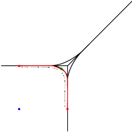
Figure 11. The simplex $\overline{S}_{+},$ drawn in red on the amoeba of $\widetilde{\mathcal{P}}_{1},$ with its barycenter illustrated in green. Note that the vertices of $\overline{S}_{+}$ are the closest points on their respective legs to the origin (blue). The arrows indicate Liouville flow along $\overline{S}_{+}.$

Theorem 5.3.4 ([N4]).

Let $\partial^{0}\widetilde{\mathcal{A}}_{n-1}^{\ell}\subset\widetilde{\mathcal{A}}_{n-1}^{\ell}$ be the component which bounds the region of $\mathbb{R}^{n}$ containing the all-negative orthant. Let $C=\operatorname{Log}^{-1}(\partial^{0}\widetilde{\mathcal{A}}_{n-1}^{\ell})\subset(\mathbb{C}^{\times})^{n}$.

Then $C$ is a contact hypersurface, and the skeleton of $\widetilde{\mathcal{P}}_{n-1}^{\ell}$ is $C\cap(-\mathbb{L}_{n})$

Proof.

We proceed by induction on the dimension of the pants, the case $n=1$ being trivial. Many of the ideas of the proof can be seen in the illustration of Figure 11.

Let us consider the legs of $\widetilde{\mathcal{P}}_{n-1}^{\ell}$. From Lemma 5.3.1, it is clear that any zero of the Liouville vector field contained in the leg $L_{i}$ must be contained inside the zero-section, i.e., the unit circle, of its $\mathbb{C}^{\times}_{i}$ factor; in other words, any zero of the Liouville vector field on $L_{i}$ must project under the $\operatorname{Log}$ map to the $i$th coordinate hyperplane in $\mathbb{R}^{n}.$ In particular, no vanishing happens on the $(n+1)$th leg of the pants, since any vanishing must be contained in the hyperplane given by the sum of the coordinate directions, and the translation by $\ell$ ensures that this hyperplane is disjoint from the leg $L_{n+1}$.

Moreover, the preimage in $\widetilde{\mathcal{P}}_{n-1}^{\ell}$ of the coordinate hyperplanes in $\mathbb{R}^{n}$ is entirely contained in the legs, and stable under the Liouville flow. By Lemma 5.3.1 and the induction hypothesis, the portion of the skeleton contained in $L_{i}$ is $(-\mathbb{L}_{n-1}\times(T^{*}_{S^{1}}S^{1})_{i})\cap C$, using the notation of Equation (2) of Example 4.1.2. By comparing that equation to the statement of this theorem, we see that our remaining task is to show there is exactly one more component of the skeleton, and to identify it with the intersection of $C$ with the positive real points of $\widetilde{\mathcal{P}}_{n-1}^{\ell}$.

Away from the legs of the pants $\widetilde{\mathcal{P}}_{n-1}^{\ell}$, the map $\operatorname{Log}$ is a local diffeomorphism everywhere except the real points $R:=\widetilde{\mathcal{P}}_{n-1}^{\ell}\cap\mathbb{R}^{n}$. Let $z=(z_{1},\ldots,z_{n})\in R$ be a real point where the Liouville vector field vanishes. The equation of the pants $\sum e^{-\ell_{i}}z_{i}=1$ prevents all $z_{i}$ from being negative; if $z_{i}$ is positive and $z_{j}$ is negative, then the Liouville vector field will point partially in the direction of $(z_{1},\ldots,z_{i}+\epsilon,\ldots,z_{j}-\epsilon,\ldots,z_{n})$ and in particular will be nonzero at $z$. Thus $z\in R_{+}=\widetilde{\mathcal{P}}_{n-1}^{\ell}\cap(\mathbb{R}_{>0})^{n}$. In order that $z$ not lie in the legs, it must be contained in

$$S_{+}=\{z\in R_{+}\mid\operatorname{Log}(z)\in(\mathbb{R}_{>0})^{n}\}.$$

Recall that $\operatorname{Log}$ restricts to a diffeomorphism $R_{+}\to\partial^{0}\widetilde{\mathcal{A}}^{\ell}_{n-1}$ from $R_{+}$ to the inner boundary component of the tailored amoeba.

Since $S_{+}$ is contained inside the real points of $\widetilde{\mathcal{P}}_{n-1}^{\ell}$, the Liouville form vanishes on its tangent vectors, so it is preserved by the Liouville vector field. The Liouville flow increases distance to $0\in\mathbb{R}^{n}$ under the Log projection, and the embedding of $\operatorname{Log}(S_{+})$ in $\mathbb{R}^{n}$ is concave and symmetric under exchange of coordinates. Hence the Liouville field everywhere points along $S_{+}$ toward the barycenter of $S_{+}$. This barycenter gives the sole remaining zero of the Liouville form, and it contributes its stable cell $S_{+}$ to the skeleton. ∎

Remark 5.3.5.

The closure $\overline{S}_{+}$ of the region $S_{+}$ is an $(n-1)$ simplex, each facet of which is contained in one of the legs, and whose boundary projects to the intersection of the amoeba with the coordinate hyperplanes. The case $n=2$ is depicted in Figure 11.

5.3.2. Skeleta for $P$-pants

Let $P=\operatorname{Conv}(0,v_{1},\ldots,v_{k})\subset M_{\mathbb{R}}^{\vee}$ be a simplex. In Definition 5.1.4, we described the $P$-pants $\widetilde{\mathcal{P}}_{P}\subset\mathbb{T}^{\vee}_{\mathbb{C}}$ obtained as a cover of the pants $\mathcal{P}_{n-1}$, and in Definition 5.2.3 we described its tailored translated version $\widetilde{\mathcal{P}}_{n-1}$.

After choosing an inner product on $M_{\mathbb{R}}$ and hence respective symplectic and Liouville forms $\omega$ and $\lambda$ on $\mathbb{T}^{\vee}_{\mathbb{C}}\cong T^{*}\mathbb{T}^{\vee}$, we can restrict these to the translated tailored $P$-pants $\widetilde{\mathcal{P}}_{P}^{\ell}$ to equip this space with the structure of a Liouville manifold. As for the standard pants, we will be interested in computing the Lagrangian skeleton of $(\widetilde{\mathcal{P}}_{P}^{\ell},\lambda),$ closely following the calculation in Theorem 5.3.4.

let $\Sigma_{P}$ be the stacky fan whose primitives are the nonzero vertices of $P$. As in the statement of Theorem 5.3.4, let $\partial^{0}\mathcal{A}_{P}^{\ell}$ be the component of the amoeba boundary $\partial\mathcal{A}_{P}^{\ell}$ bounding the “lower-left” orthant of $\mathbb{R}^{n}$. We will be interested in the contact hypersurface $C_{P}\subset\mathbb{T}_{\mathbb{C}}^{\vee}$ lying above this boundary:

$$C_{P}:=\{z\in\mathbb{T}_{\mathbb{C}}^{\vee}\mid\operatorname{Log}(z)\in\mathcal{A}_{P}^{0}\}.$$

As in Section 4, let $G_{\sigma}$ be the possibly disconnected torus $\textup{Hom}(M^{\vee}_{\sigma},\mathbb{R}/\mathbb{Z}),$ where $M^{\vee}_{\sigma}$ is the quotient of $M^{\vee}$ by the vertices of the stacky primitives in $\sigma.$ This defines a Lagrangian

$$\mathbb{L}_{\Sigma_{P}}:=\bigcup_{\sigma\in\Sigma_{P}}G_{\sigma}\times\sigma\subset T^{*}\mathbb{T}^{\vee};$$

using the inner product, we can treat $\Sigma$ as a fan of cones in $M_{\mathbb{R}}$ and hence $\mathbb{L}_{\Sigma_{P}}$ as a subset of $\mathbb{T}^{\vee}_{\mathbb{C}}.$

For $1\leq i\leq k,$ write $\Sigma_{P}^{i}$ for the fan of cones on the $(k-1)$ vectors $v_{1},\ldots,v_{\hat{i}},\ldots,v_{k}.$ As was the case for the standard pants, we find it helpful to rewrite the FLTZ Lagrangian as a union

$$\mathbb{L}_{\Sigma_{P}}=(G_{\Sigma_{P}}\times\Sigma_{P})\bigcup_{1\leq i\leq k}\mathbb{L}_{\Sigma_{P}^{i}}$$

of one new piece (where we write $\Sigma_{P}$ for the big cone in the fan), living in the cotangent fibers over the points $G_{\Sigma_{P}},$ and FLTZ skeleta for lower-dimensional cones of $\Sigma$.

Lemma 5.3.6.

There is an equality

$$\Lambda_{P}=C_{P}\cap(-\mathbb{L}_{\Sigma_{P}})$$

between the skeleton $\Lambda_{P}$ of $\widetilde{\mathcal{P}}^{\ell}_{P}$ and the intersection of the contact hypersurface $C_{P}$ with the negative stacky FLTZ Lagrangian for $\Sigma_{P}.$

Proof.

The proof of Theorem 5.3.4 proceeded by induction on dimension, using the fact that each leg $L_{i}$ of the stnadard pants was itself (the product of $\mathbb{C}^{\times}$ with) a pants one dimension lower. The proof here follows the same strategy: we need to consider here $P$-pants for all $P$ (not necessarily top-dimensional), but as before we induct on the dimension of $P$.

For clarity, we spell out explicitly the base case, when $P=\operatorname{Conv}(0,v)$ is 1-dimensional. In this case, the tailoring construction is unnecessary, since $\mathcal{P}_{P}^{\ell}$ is the hypersurface defined (in coordinates $z=(z_{1},\ldots,z_{n})$) by $\{z_{1}^{v_{1}}\ldots z_{n}^{v_{n}}=e^{\ell}\},$ whose amoeba $\operatorname{Log}(\mathcal{P}_{P}^{\ell})$ is the hyperplane

$$\mathcal{A}_{P}^{\ell}=\{v_{1}x_{1}+\cdots v_{n}x_{n}=\ell\}\subset\mathbb{R}^{n}\cong M_{\mathbb{R}}.$$

In other words, the hypersurface $\mathcal{P}_{P}^{\ell}$ is a copy of $(\mathbb{C}^{\times})^{n-1}$, with its symplectic and Liouville form restricted from those of the ambient $(\mathbb{C}^{\times})^{n}.$ Hence its Liouville vector field is given by the gradient of the restriction of the Morse-Bott function $|\operatorname{Log}|^{2}.$ The critical locus of this function is the fiber of $\mathcal{P}_{P}^{\ell}$ over the point $p\in\mathcal{A}_{P}^{\ell}$ nearest to $0\in M_{\mathbb{R}},$ which is a manifold of minima for $|\operatorname{Log}|^{2}|_{\mathcal{P}_{P}^{\ell}}.$ As $v$ is the normal vector to the hyperplane $\mathcal{A}_{P}^{\ell},$ the point $p$ is the point of $\widetilde{\mathcal{A}}_{P}^{\ell}$ where it intersects the ray defined by $v.$ The fiber over this point is the preimage, under the covering map $f_{A},$ of the corresponding fiber of the standard pants: this is the subtorus $G_{v}\subset\mathbb{T}^{\vee}.$

We now assume by induction that we have proven the lemma for all $P^{\prime}$-pants with $\dim(P^{\prime})<n,$ and we return to the case where $P=\operatorname{Conv}(0,v_{1},\ldots v_{n})$ is an $n$-simplex. From this point the proof follows very closely the proof for the standard pants. As in that case, we first investigate the legs $L_{1},\ldots,L_{n}$ of $\widetilde{\mathcal{P}}_{P}^{\ell}.$ Each of these is itself a $P^{\prime}$-pants, for $P^{\prime}=\operatorname{Conv}(0,v_{1},\ldots,v_{\hat{i}},\ldots,v_{n}),$ and by induction we know that the vanishing of the Liouville vector field on leg $L_{i}$ contributes to the skeleton of $\widetilde{\mathcal{P}}_{P}^{\ell}$ the piece $\mathbb{L}_{\Sigma_{P}^{i}}\cap C_{P}$. It remains for us to determine the vanishing loci of the Liouville vector field on the interior of the pants. (As for the standard pants, it is obvious that no vanishing happens on the final leg.)

We now consider the simplex $\overline{S}_{+}=\partial^{0}\widetilde{\mathcal{A}}_{P}\cap\Sigma_{P},$ where we write $\Sigma_{P}$ for the top-dimensional cone in the fan, and we write $p\in\overline{S}_{+}$ for the point in the interior of $\overline{S}_{+}$ which is closest to 0. Let $S_{+}$ denote the preimage of the interior of this simplex, which is now a disjoint union $S_{+}=\bigsqcup_{i=1}^{d}S_{+}^{i}$ of $d=\operatorname{vol}(P)$ open simplices $S_{+}^{i}.$ Each of these simplices is preserved by the Liouville flow, which flows each simplex to the point lying over $p$, on which the Liouville field vanishes. Hence the remaining pieces of the skeleton are the open simplices $S^{i}_{+},$ each of which is mapped diffeomorphically by $\operatorname{Log}$ onto the interior of $\overline{S}_{+}.$ As $\overline{S}_{+}$ is the intersection of $\partial^{0}\widetilde{\mathcal{A}}_{P}$ with the big cone in $\Sigma_{P},$ and the fiber in $\widetilde{\mathcal{P}}_{P}^{\ell}$ over a point in $\overline{S}_{+}$ is the discrete group $G_{\Sigma}$, this is the desired extra piece in $\mathbb{L}_{\Sigma_{P}}\cap C_{P}.$

Finally, if there were any other vanishing of the Liouville form in the interior of the pants, it would have to lie over a critical value of $\operatorname{Log}$. These critical values are just the preimage (under the cover $f_{A}$) of the real points of $\widetilde{\mathcal{P}}_{n-1},$ and we have already seen in the proof of Theorem 5.3.4 that the Liouville vector field is nonvanishing there. ∎

A crucial point is that the above result holds in the case of a simplex $P$ with arbitrary volume, obtained as a cover of the standard simplex $\Delta_{n-1}.$ For instance, when $n=2$, the $P$-pants $\widetilde{\mathcal{P}}_{P}$ may be higher genus.

Example 5.3.7.

Let $\Delta\subset\mathbb{R}^{2}$ be the simplex with vertices $\{(0,0),(2,0),(0,2)\},$ so that the corresponding stacky fan $\Sigma$ is a stacky fan for the stack $\mathbb{A}^{2}/(\mathbb{Z}/2\times\mathbb{Z}/2).$ We draw the stacky fan and FLTZ skeleton in Figure 12. The boundary $\partial\mathbb{A}^{2}/(\mathbb{Z}/2\times\mathbb{Z}/2)$ matches the mirror skeleton pictured in Figure 13.

                  

Figure 12. The stacky fan and FLTZ skeleton for $\mathbb{A}^{2}/(\mathbb{Z}/2\times\mathbb{Z}/2)$.

Figure 13. The skeleton $\mathbb{L}_{\Delta}$ of the pants $\widetilde{\mathcal{P}}_{\Delta}$ associated to the simplex $\Delta$ with vertices $(0,0),(2,0),(0,2),$ and its 4:1 cover of the skeleton of the standard pants.

6. Patchworking and skeleta

Fix a complex torus $\mathbb{T}^{\vee}_{\mathbb{C}}=T\mathbb{T}^{\vee}$, along with a toric partial compactification $\mathbf{T}_{\Sigma}$ arising from a (stacky) fan $\Sigma\subset M^{\vee}_{\mathbb{R}}$. We write $\Delta^{\vee}$ for the convex hull of the stacky primitives.

According to [HV], the mirror to $\mathbf{T}_{\Sigma}$ is the Landau-Ginzburg model associated to a function $W_{\Sigma}:\mathbb{T}^{\vee}_{\mathbb{C}}\to\mathbb{C}$ whose Newton polytope is $\Delta^{\vee}$. In addition, the expected mirror to $\partial\mathbf{T}_{\Sigma}$ is a general fiber $F_{W}$ of $W_{\Sigma}$.

In this section we will explain how $W_{\Sigma}$ determines a Liouville sector (i.e. prove Prop. 2.3.1) and show that the relative skeleton of this sector is the FLTZ Lagrangian $\mathbb{L}_{\Sigma}$.

Let us briefly outline the ideas involved. We will study the hyperplane $F_{W}$ through its amoeba ([GKZ]), the projection of $\partial\mathbf{T}^{mir}$ to the tangent fiber:

$$\mathcal{A}:=\operatorname{Log}(\partial\mathbf{T}^{mir})\subset M_{\mathbb{R}}.$$

The cones of $\Sigma$ give a triangulation of the polytope $\Delta^{\vee}$. We choose the Laurent polynomial $W_{\Sigma}$ so that its tropicalization $\Pi_{\Sigma}$ is a spine onto which $\mathcal{A}$ retracts. The complex $\Pi_{\Sigma}$ is a piecewise-affine locus dual to the triangulation of $\Delta^{\vee}$ by the cones of $\Sigma$. By assumption, this triangulation is star-shaped (all non-boundary simplices share a common vertex 0); the distinguished vertex corresponds to a distinuished component of the complement of the amoeba. We denote the boundary of this region by $\partial^{0}\mathcal{A}\subset\partial\mathcal{A}$.

Mikhalkin [M] shows how to isotope the hypersurface $F_{W}$ to another hypersurface $F_{\Sigma}$ whose amoeba is “close” to the spine $\Pi_{\Sigma}.$ As we have recalled in Sections 5.2 and 5.3, this isotopy was used by Nadler [N4] to compute the skeleton of the “$n$-dimensional pants”, i.e., the zero locus of the polynomial $W_{\Sigma}=1+\sum_{i=1}^{n}z_{i}$.

In our more general setting, Mikhalkin’s isotopy ensures that the critical points of $\operatorname{Log}|_{F_{\Sigma}}$ – and in fact the entire skeleton $\mathbb{L}_{\Sigma}$ – lie above the distinguished boundary component $\partial^{0}\mathcal{A}$ of the amoeba. The preimage of such a boundary component is precisely a contact type hypersurface. Finally, to each pants in the decomposition of $F_{\Sigma}$ we apply the argument from [N4] described in the previous section to obtain the precise form of the skeleton.

6.1. Pants decomposition of $F_{\Sigma}$

In order to construct $F_{\Sigma}$ and produce its skeleton, we will follow [N4] in using Mikhalkin’s theory of localized hypersurfaces, which we now recall.

6.1.1. Triangulation and dual complex

Recall that we are assuming the fan $\Sigma$ is smooth and quasi-projective, or equivalently, that the subdivision $\mathcal{T}$ of $\Delta^{\vee}$ is a regular triangulation. By definition, regularity of $\mathcal{T}$ means that $\mathcal{T}$ is the corner locus of a convex piecewise-linear function $\alpha:\Delta^{\vee}\cap M^{\vee}\to\mathbb{R}$. The Legendre transform of $\alpha$ is the function

Definition 6.1.1.

The dual complex for the regular triangulation $\mathcal{T}$ is the polyhedral complex in $M_{\mathbb{R}}$ obtained as the corner locus of the Legendre transform $L_{\alpha}$. We will denote the dual complex for $\mathcal{T}$ by $\Pi_{\Sigma}.$

Example 6.1.2.

Let $e_{1},\ldots,e_{n}$ be a basis of $M^{\vee},$ and let $\Delta_{std}^{\vee}$ be the polytope with vertices $0,e_{1},\ldots,e_{n}.$ Then we can define a piecewise-linear function $\alpha$ on $\Delta_{std}^{\vee}$ by declaring $\alpha(0)=0,\alpha(e_{i})=\alpha_{i}$ for some $\alpha_{i}>0$. The resulting dual complex $\Pi_{std}$ is the corner locus of the function $(a_{1},\ldots,a_{n})\mapsto\max(0,a_{1}-\alpha_{1},\ldots,a_{n}-\alpha_{n})$; in other words, it is a translation by $(\alpha_{1},\ldots,\alpha_{n})$ of the tropical pants $\Pi_{n-1}$ defined in Section 5.1.

The geometric significance of $\Pi_{\Sigma}$ is the following. Recall that the amoeba of a hypersurface in $(\mathbb{C}^{\times})^{n}$ is its image in $\mathbb{R}^{n}$ under the map

Proposition 6.1.3.

[M] Let $V$ denote the set of vertices in the triangulation $\mathcal{T},$ and let $H^{t}=\{f^{t}=0\},$ where

$$f^{t}=\sum_{m\in V}t^{-\alpha(m)}z^{m}.$$

For $t\gg 0$, the complex $\Pi_{\Sigma}\cdot\log(t)$ will sit as a spine inside the amoeba of $\operatorname{Log}(H_{t})$, and as $t\to\infty,$ the rescaled amoebae $\operatorname{Log}(H_{t})/\log(t)$ converge (Gromov-Hausdorff) to $\Pi_{\Sigma}.$

Proof.

The basic idea is as follows. Consider a face $E$ of the dual complex $\Pi_{\Sigma}$, corresponding to a face $E^{\vee}$ of the triangulation $\mathcal{T}$. Then the portion of the amoeba lying over the interior of $E$ is a region where the behavior of $f_{t}$ is dominated by those monomials in $f_{t}$ corresponding to vertices of $E^{\vee}$. See [M, Section 6] for details. ∎

One says that the complex $\Pi_{\Sigma}$ is the tropical hypersurface associated to the Newton polytope $\Delta^{\vee}$ with regular triangulation $\mathcal{T}.$ We term $t$ the ‘tropicalization parameter’.

Figure 14. A maximal subdivision of the polygon with vertices $(-1,0),(0,-1),(1,1)$, and its (unimodular) dual complex $\Pi.$

Since the triangulation $\mathcal{T}$ of $\Delta^{\vee}$ is star-shaped, we have:

Lemma 6.1.4.

Let $\Pi_{\Sigma}^{0}$ be the component of $M_{\mathbb{R}}\setminus\Pi_{\Sigma}$ corresponding to the vertex 0 of the triangulation $\mathcal{T}$, and denote its boundary by $\partial^{0}\Pi_{\Sigma}.$ The polytope $\Pi^{0}_{\Sigma}$ is a (possibly unbounded) polytope with face poset anti-equivalent to the poset of nonzero cones in the fan $\Sigma.$

The polytope $\Pi_{\Sigma}^{0}$ will be bounded if and only if the toric variety $\mathbf{T}_{\Sigma}$ is proper, in which case $\Pi_{\Sigma}^{0}$ will be the only bounded polytope in $M_{\mathbb{R}}\setminus\Pi^{0}_{\Sigma}.$

6.1.2. Tropical pants

We required the subdivision $\mathcal{T}$ of $\Delta^{\vee}$ to be a triangulation, which means that all of the faces in $\mathcal{T}$ are simplices. This allows us to divide up $\Pi_{\Sigma}$ into pieces we understand:

Definition 6.1.5.

The neighborhood in $\Pi_{\Sigma}$ of any vertex is a tropical pants.

These pants will be our basic building blocks in the construction to follow. This has two appealing features: the first is that the complex $\Pi_{\Sigma}$ is obtained by gluing these pants together. Second, a $(k-1)$-face in $\Pi_{\Sigma}$ is the product of $\mathbb{R}^{k}$ with a $(n-k-1)$-dimensional tropical pants. Hence the loci along which pants involved in the description of $\Pi_{\Sigma}$ are glued are products of the form $(\text{lower-dimensional pants})\times\mathbb{R}^{k}$.

6.1.3. Tailoring

We now recall the construction of [M] giving an isotopy from $F_{W}$ to some $F_{\Sigma}$ whose amoeba is closer to the tropical hypersurface $\Pi_{\Sigma}$. In the case of the pants $\mathcal{P}_{n-1},$ this isotopy was described in Proposition 5.2.1 above.

It is straightforward to see what $F_{\Sigma}$ should be. Suppose two simplices $P_{1},P_{2}$ in the triangulation $\mathcal{T}$ share a common face $F$, so that their respective dual complexes $\Pi_{P_{1}},\Pi_{P_{2}}$ overlap in a common subcomplex $\Pi_{F}$, and let $U$ be a neighborhood of the interior of $\Pi_{F}.$ Then the inductive structure of the tailored $P$-pants ensures that above $U$, the pants $\widetilde{\mathcal{P}}_{P_{1}}$ and $\widetilde{\mathcal{P}}_{P_{2}}$ agree: both are equal to the tailored leg $\widetilde{\mathcal{P}}_{F}.$ Thus we may take the union of all these pants to define $F_{\Sigma}$.

The isotopy can be glued similarly:

Lemma 6.1.6 ([M, Section 6.6], [A1, Propositions 4.2, 4.9]).

There is a Hamiltonian isotopy of symplectic hypersurfaces $F_{W}\to F_{\Sigma}$ such that for each face $F$ in the tropical curve $\Pi_{\Sigma}\subset M_{\mathbb{R}}$, corresponding to a polytope $P$ in the triangulation $\mathcal{T}$, there is a neighborhood $U_{P}\subset M_{\mathbb{R}}$ such that $\operatorname{Log}^{-1}(U_{v})$ is equal to the intersection $\widetilde{\mathcal{P}}_{P}^{\ell}$ with a large ball in $\mathbb{T}_{\mathbb{C}}^{\vee}.$

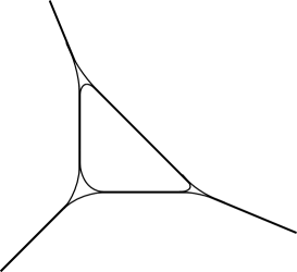
Figure 15. The amoeba of the localization of the hypersurface $xy+\frac{1}{x}+\frac{1}{y}=0.$

Remark 6.1.7.

The symplectic isotopy from [A1] is defined as follows: for $t\geq 0$ and $0\leq s\leq 1,$ write $H^{t,s}=\{f^{t,s}=0\},$

(8) $$f^{t,s}:=\sum_{m}t^{-\alpha(m)}(1-s\phi_{m}(\operatorname{Log}(z)))z^{m},$$

where the sum is taken over the vertices of the triangulation $\mathcal{T}$ of $\Delta^{\vee},$ and $\phi_{m}\in C^{\infty}(\mathbb{R}^{n})$ is a certain function which is 1 in a neighborhood of the component of $M_{\mathbb{R}}\setminus\Pi_{\Sigma}$ corresponding to $m,$ and 0 away from that region; as in Section 6.1.1, taking the tropicalization parameter $t$ large ensures that $\operatorname{Log}(H^{t,s})$ contains $\log(t)\cdot\Pi_{\Sigma}$ as a spine. Taking the “tailoring parameter” $s$ from 0 to 1 deforms the hypersurface $\{\sum_{m}t^{-\alpha(m)}z^{m}\}$ by forcing that, on each region of the amoeba $t$, any term which does not dominate the behavior of $f^{t,0}$ in that region (as described in the proof of Proposition 6.1.3) does not contribute at all.

Remark 6.1.8.

As in our definition of the standard pants, our convention in this paper will differ from that in Equation (8) by our choice to take the sign of the constant coefficient of $f^{t,s}$ to be negative rather than positive. This ensures that the real positive points of $H^{t,s}$ lie over the boundary of the central component of the amoeba complement.

6.2. The skeleton of $F_{\Sigma}$

As in Section 5.3, by choosing an inner-product on $M$, we obtain an isomorphism $\mathbb{T}_{\mathbb{C}}^{\vee}=T\mathbb{T}^{\vee}\cong T^{*}\mathbb{T}^{\vee},$ and we restrict the symplectic form $\omega,$ and its primitive $\lambda$ from this space to $F_{\Sigma}$. We will use the pants decomposition of $F_{\Sigma}$ to (observe that it is a Liouville manifold and) compute its skeleton, which we denote by $\Lambda_{\Sigma}.$

However, in order to avoid performing any calculations beyond those described so far, we must adopt a certain technical hypothesis on the fan $\Sigma$. As remarked in the introduction, this hypothesis can be removed; see [Z] for details.

Definition 6.2.1.

A polytope $P\subset M_{\mathbb{R}}^{\vee}$ is called perfectly centered if for each nonempty face $F\subset P,$ the normal cone of $F$ (transported to $M_{\mathbb{R}}^{\vee}$ by the inner product $M_{\mathbb{R}}^{\vee}\cong M_{\mathbb{R}}$) has nonempty intersection with the relative interior of $F$.

As in the proof of Lemma 2.5.3, we write $\alpha:\Delta^{\vee}\to\mathbb{R}$ for a function inducing the regular triangulation of $\Delta^{\vee}$ defined by $\Sigma.$ The complex $\Pi_{\Sigma}$ depends on our choice of $\alpha$.

Definition 6.2.2.

We will say that a fan $\Sigma$ is PC if there exists some $\alpha$ as above for which the polytope $\Pi_{\Sigma}^{0}$ is perfectly centered.

Assume now that the fan $\Sigma$ is PC.

Remark 6.2.3.

So far, no fan is known to us not to be PC; nor, however, do we know any compelling reason why all fans should be PC.

We will denote the amoeba of $F_{\Sigma}$ by

$$\widetilde{\mathcal{A}}_{\Sigma}:=\operatorname{Log}(F_{\Sigma}).$$

Recall that we write $\Pi^{0}_{\Sigma}$ for the component of $M_{\mathbb{R}}\setminus\Pi_{\Sigma}$ dual to the unique 0-dimensional cone in $\Sigma$ and $\partial^{0}\Pi_{\Sigma}$ for its boundary. Write $\partial^{0}\widetilde{\mathcal{A}}_{\Sigma}$ for the corresponding boundary component of the amoeba, and

Recall that we write $-\mathbb{L}_{\Sigma}=\bigcup_{0\neq\sigma\in\Sigma}\sigma^{\perp}\times\sigma$ for the (negative) FLTZ skeleton.

Theorem 6.2.4.

The skeleton $\Lambda_{\Sigma}$ of $\partial\mathbf{T}^{mir}_{loc}$ can be written as the intersection

Proof.

From our hypothesis that the fan $\Sigma$ is PC, we may assume that the polytope $\Pi_{\Sigma}^{0}$ is perfectly centered, so that each nonzero cone $\sigma$ in $\Sigma$ intersects its dual face in $\Pi_{\Sigma}^{0}$, as in Figure 16. This allows us to define an open cover of $F_{\Sigma}$ as follows: for each top-dimensional cone $\sigma$ in $\Sigma$, let $V_{\sigma}$ be a neighborhood of the cone $\sigma,$ thought of as in $M_{\mathbb{R}}$.

Let $U_{\sigma}=\operatorname{Log}^{-1}(V_{\sigma})\cap F_{\Sigma}$ be the lift of $V_{\sigma}$ to an open subset of $F_{\Sigma}.$ Then $U_{\sigma}$ is an open subset in a pants $\widetilde{\mathcal{P}}_{\sigma}^{\ell}$. By construction, the image of $U_{\sigma}$ in $\widetilde{\mathcal{P}}_{\sigma}^{\ell}$ contains the whole skeleton $\Lambda_{\sigma}$ of $\widetilde{\mathcal{P}}_{\sigma}^{\ell}.$ On the other hand, every zero of $\lambda|_{F_{\Sigma}}$ is contained in some $U_{\tau},$ as is its stable manifold. We conclude the skeleton $\Lambda_{\Sigma}$ is equal to the union of the skeleta $\Lambda_{\tau}.$ ∎

Note $C$ is transverse to the Liouville flow on $\mathbb{T}^{\vee}$, hence contact. In addition:

Lemma 6.2.5.

In a neighborhood of the skeleton $\Lambda_{\Sigma},$ the hypersurface $F_{\Sigma}$ is nowhere tangent to the ambient Liouville vector field of the Weinstein manifold $\mathbb{T}_{\mathbb{C}}^{\vee}.$

Proof.

The pants cover of $F_{\Sigma}$ allows us to reduce to the case where $F_{\Sigma}=\widetilde{\mathcal{P}}_{P}^{\ell}$ is a $P$-pants. Now we can proceed by the induction used in the proof of Lemma 5.3.6.

In the base case, $P=\operatorname{Conv}(0,v)$ is 1-dimensional, and $\widetilde{\mathcal{P}}_{P}^{\ell}=\{z_{1}^{v_{1}}\cdots z_{n}^{v_{n}}=e^{\ell}\}$ is a copy of $(\mathbb{C}^{\times})^{n-1}$ projecting by Log to its tropical hypersurface $\Pi_{\Sigma}$. The Liouville vector field on $\mathbb{T}_{\mathbb{C}}^{\vee}=(\mathbb{C}^{\times})^{n}$, under the Log projection, points directly outward from $\Pi_{\Sigma}.$

Now suppose $P=\operatorname{Conv}(0,v_{1},\ldots,v_{n})$ is an $n$-simplex. We know the result on the legs of $\widetilde{\mathcal{P}}_{P}^{\ell}$ by induction, so we only need to prove it in a neighborhood of the big simplex $S_{+}$ in the skeleton, which is the preimage under the cover $\widetilde{\mathcal{P}}_{P}^{\ell}\to\widetilde{\mathcal{P}}_{n-1}^{\ell}$ of the positive real points of $\widetilde{\mathcal{P}}_{n-1}^{\ell}.$ But the Liouville vector field on $\mathbb{T}_{\mathbb{C}}^{\vee}=(\mathbb{C}^{\times})^{n}$ in coordinates $z_{j}=e^{\xi_{j}+i\theta_{j}}$ is $\sum_{j}\xi_{j}\partial_{\xi_{j}},$ so if $\widetilde{\mathcal{P}}_{P}^{\ell}$ had any tangent vectors along $S_{+}$ in the direction of the Liouville flow, this would imply that $\widetilde{\mathcal{P}}_{n-1}^{\ell}$ had positive real points which do not project to the boundary of the amoeba, which is false. ∎

Corollary 6.2.6.

There is a Liouville domain $D\subset\mathbb{T}^{\vee}$ completing to $\mathbb{T}^{\vee}$ and a Liouville domain $F\subset F_{\Sigma}$ completing to $F_{\Sigma}$, such that $F\subset\partial D$ and the FLTZ Lagrangian $-\mathbb{L}_{\Sigma}$ is a relative skeleton for the pair $(D,F)$.

Proof.

The point is that we may deform $C$ transversely to the Liouville flow in such a way as to cause it to contain some neighborhood $U_{\Sigma}\subset F_{\Sigma}$ of $\Lambda_{\Sigma}$.

Indeed, the Liouville flow gives an identification $T^{*}\mathbb{T}^{\vee}\setminus\mathbb{T}^{\vee}\cong C\times\mathbb{R}$, with $C$ included as $C\times 0$. By Lemma 6.2.5, for some closed manifold $V_{\Sigma}\subset F_{\Sigma}$ neighborhood of $\Lambda_{\Sigma}$, the corresponding projection $V_{\Sigma}\to C$ is an embedding. Its image is some codimension one smooth hypersurface (with boundary) of $C$, over which we may write $V_{\Sigma}$ as the graph of a smooth function. Extend this function arbitrarily to all of $C$. The graph of the result will be the boundary of our desired $D$.

We thank John Pardon for this method of constructing Liouville pairs. ∎

Example 6.2.7.

Let $\Delta^{\vee}$ be the polytope with vertices $(1,1),(0,-1),(-1,0),$ as in Figure 14 and Figure 15. In Figure 16, the fan $\Sigma$ is drawn superimposed on the amoeba $\mathcal{A}_{\Sigma}.$ A neighborhood of each top-dimensional cone in $\Sigma$ is a pair of pants which contributes to $\mathbb{L}$ a pair of circles attached by an interval. The circles live over the points where the rays of $\Sigma$ intersect $\Pi,$ and the intervals lie over the boundary of the bounded region in the center of the amoeba.

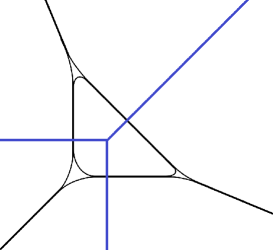
Figure 16. The fan $\Sigma$ for $\mathbb{P}^{2}$ superimposed on the amoeba $\mathcal{A}_{\Sigma}.$

7. Microlocalizing Bondal’s correspondence

Recall we denote by $\mathbb{T}$ a torus with respective character and cocharacter lattices $M$ and $M^{\vee}$. Fix a (stacky) fan $\Sigma\subset M^{\vee}_{\mathbb{R}}$ and the corresponding toric partial compactification $\mathbb{T}_{\mathbb{C}}\subset\mathbf{T}_{\Sigma}$.

Bondal [B] described a fully faithful embedding of the category of coherent sheaves on $\mathbf{T}_{\Sigma}$ into the category of constructible sheaves on the real torus $\mathbb{T}^{\vee}_{\mathbb{R}}:=M\otimes\mathbb{R}/\mathbb{Z}$. This was developed further in [FLTZ2, FLTZ3, Tr]; in particular, the constructible sheaves in question were observed to have microsupport contained in $\mathbb{L}_{\Sigma}$ and conjectured to generate the category of such sheaves. This conjecture was established in [Ku].

We use this equivalence to prove a similarly-flavored equivalence “at infinity”, i.e., an equivalence between the category of coherent sheaves on the toric boundary and the category of wrapped microlocal sheaves away from the zero section.

Categories and conventions — We work with dg categories over a fixed ground ring $k$. This theory can be set up either directly [Kel1, Kel2, Dr] or by specializing the theory of stable $(\infty,1)$-categories of [Lur1, Lur2] as in [GR, I.1.10].

The microlocal sheaf theory of [KS] was originally developed in the setting of the bounded derived category. It is essential for our work here to work with the dg category of unbounded complexes. It is well known to experts that it is straightforward to set up the sheaf theory in this setting (see e.g. [N1, Sec. 2.2] or [GPS3, Sec. 4.1]) and that, with the use of [Spa, RS] to deal with some issues around unbounded complexes, all constructions of [KS] may be translated to this setting.

For a manifold $M$, we write $Sh(M)$ for the unbounded dg derived category of sheaves of $k$-modules on $M$. We impose no restrictions on the stalks; i.e., we write $Sh$ for what in [N4] is called $Sh^{\diamond}$ (and similarly for the later $\mu sh$).

For a conical subset $Z\subset T^{*}M$, we write $Sh_{Z}(M)$ for the full subcategory of $Sh(M)$ consisting of those sheaves with microsupport in $Z$. When $Z$ is subanalytic Lagrangian, then this subcategory is compactly generated, and we write $Sh_{Z}(M)^{c}$ for the subcategory of compact objects. This subcategory is generally larger than the category of sheaves with perfect stalks in $Sh_{Z}(M)$; for instance, when $Z=\emptyset$ it contains the tautological (derived) local system with fiber $C_{*}(\Omega M)$. The idea to use compact objects in the unbounded category to model the wrapped Fukaya category stopped at $Z$ is due to Nadler [N4]; that it works is now a theorem [GPS3]. The reader is referred to these articles for further discussions of this category.

For $X$ an algebraic variety (or stack), we write $\textup{QCoh}(X)$ for the dg derived category of quasi-coherent sheaves on $X$ in the sense of [GR]; as observed there, the bounded subcategory agrees with the usual usage of this term. It is useful to remember that perfect complexes (bounded complexes of projectives) are precisely the compact objects in $\textup{QCoh}(X)$, which can be recovered from $\textup{Perf}(X)$ by ind-completion. Similarly, we will write $\textup{IndCoh}(X)$ for the Ind-completion of the category $\textup{Coh}(X)$ of coherent sheaves on $X$ ([GR]). We can recover the category $\textup{Coh}(X)$ by passing to compact objects.

To simplify notation, we write as if $\Sigma$ is an ordinary (non-stacky) fan. To arrive at the corresponding statements in the stacky case, one need merely remember the data of a finite abelian group $\Gamma_{\sigma}$ for each cone in $\sigma$, and correspondingly replace the sets $\{A(\sigma)\}_{\sigma\in\Sigma},$ $\{B(\sigma)\}_{\sigma\in\Sigma}$ with sets $\{A(\sigma,\chi)\}_{\sigma\in\Sigma,\chi\in\Gamma_{\sigma}}$, $\{B(\sigma,\chi)\}_{\sigma\in\Sigma,\chi\in\Gamma_{\sigma}},$ where the added $\chi$ denotes translation in $\mathbb{T}^{\vee}$ and twists by a character, respectively. See [FLTZ3, Section 5] for details.

7.1. Bondal’s coherent-constructible correspondence

For a cone $\sigma\subset M^{\vee}$, we write $B(\sigma)$ for the structure sheaf on $\textup{Spec}(k[\sigma^{\vee}])$, or its pushforward to any toric variety whose fan contains the cone $\sigma$. On the other hand, we write $A(\sigma)$ for the constructible sheaf on $M\otimes\mathbb{R}/\mathbb{Z}$ obtained by taking the $!$-pushforward of the dualizing (constructible) sheaf on the interior of $\sigma^{\vee}$. One then makes the following

Basic calculation ([B, FLTZ2, Tr]): Let $\mathbf{T}_{\Sigma}$ be a toric variety with fan $\Sigma$, with dense torus $\mathbb{T}_{\mathbb{C}}.$ Let $\sigma,\tau\in\Sigma$ be cones. Then there are canonical isomorphisms

$$H^{*}\textup{Hom}(A(\sigma),A(\tau))\cong k[\tau^{\vee}]\cong H^{*}\textup{Hom}(B(\sigma),B(\tau))\qquad\qquad\mbox{if}\,\,\sigma\supset\tau,$$

and all other Homs between such objects vanish. This is moreover compatible with the evident composition structure.

We denote full dg subcategories generated by the $A(\sigma)$ and $B(\sigma)$ by

$$A_{\Sigma} := \{A(\sigma)\,|\,\sigma\in\Sigma\}\subset Sh(\mathbb{T}^{\vee}),$$

$$B_{\Sigma} := \{B(\sigma)\,|\,\sigma\in\Sigma\}\subset QCoh(\mathbf{T}_{\Sigma}).$$

While the calculation above might seem to imply only the equivalence $H^{0}(A_{\Sigma})\cong H^{0}(B_{\Sigma})$ of triangulated categories, we recall the following useful fact:

Lemma 7.1.1.

Let $\mathcal{C}_{i}$ be a collection of dg categories, each of which has all morphisms concentrated in cohomological degree zero. Then any diagram valued in the $H^{0}(\mathcal{C}_{i})$ lifts canonically to a homotopy coherent diagram in the corresponding $\mathcal{C}_{i}$.

Proof.

The hypothesis on $\mathcal{C}_{i}$ implies that the natural maps

are quasi-isomorphisms. Thus any diagram among the $H^{0}(\mathcal{C}_{i})$ can be lifted to a diagram among the $\mathcal{C}_{i}$ by composing with this pair of quasi-isomorphisms. ∎

As the category of quasicoherent sheaves on a toric variety is generated by the structure sheaves of the affine toric charts, the restriction to the subcategory $B_{\Sigma}$ is really no restriction: the morphism $QCoh(\mathbf{T}_{\Sigma})\to\textup{Mod}-B_{\Sigma}$ is an isomorphism.

On the other side, the objects of $A_{\Sigma}$ all satisfy the microsupport estimate

$$ss(A(\tau))\subset\bigcup_{\sigma\subset\tau}\sigma^{\perp}\times(-\sigma)\subset\mathbb{T}^{\vee}\times M^{\vee}_{\mathbb{R}}=T^{*}\mathbb{T}^{\vee}.$$

In particular, writing

$$\mathbb{L}_{\Sigma}:=\bigcup_{\sigma\in\Sigma}\sigma^{\perp}\times(-\sigma),$$

we have that $A_{\sigma}\in Sh_{\mathbb{L}_{\Sigma}}(\mathbb{T}^{\vee})$ for all $\sigma\in\Sigma$. As conjectured by [FLTZ, Tr], and proven by Kuwagaki [Ku], these objects generate this category:

Theorem 7.1.2.

[Ku] When $\mathbf{T}_{\Sigma}$ is a smooth orbifold, the morphism $Sh_{\mathbb{L}_{\Sigma}}(\mathbb{T}^{\vee})\to\textup{Mod}-A_{\Sigma}$ is an isomorphism.

Remark 7.1.3.

In fact what Kuwakagi proves is that for any, not necessarily smooth, $\mathbf{T}_{\Sigma}$ there is an isomorphism $Sh_{\mathbb{L}_{\Sigma}}(\mathbb{T}^{\vee})\cong IndCoh(\mathbf{T}_{\Sigma})$. The above statement follows because in the smooth case, $IndCoh=QCoh$, which as we mentioned above is generated by the $B_{\sigma}$. We use the above formulation rather than Kuwagaki’s more general result because we will later make calculations with the $A_{\sigma}$ and $B_{\sigma}$ directly, and we restrict ourselves to the smooth case to avoid e.g. worrying about how to lift the $B_{\sigma}$ to $IndCoh$.

This causes no loss of generality, since it is anyway only in the smooth case that we have been able to identify $\partial\mathbb{L}_{\Sigma}$ as a relative skeleton.

7.2. Restriction is mirror to microlocalization

Let $\mathbf{T}$ be a toric variety, $\sigma$ a cone of the fan $\Sigma(\mathbf{T})$, and $i_{\sigma}:\overline{O(\sigma)}\to\mathbf{T}$ the inclusion of the orbit closure corresponding to the cone $\sigma$. As the orbit closure is itself a toric variety, one can ask what functor of constructible sheaf categories corresponds under Bondal’s correspondence to the pullback $i_{\sigma}^{*}.$ We will see that the answer is a sort of microlocalization functor.

7.2.1. Restriction to orbit closures

Recall that the orbit closure $\overline{O(\sigma)}$ carries the structure of a toric variety, with associated cocharacter lattice $M^{\vee}/\mathbb{Z}\sigma$. For $\tau$ a cone containing $\sigma$, we write $\tau/\sigma$ for the image of $\tau$ in $M^{\vee}/\mathbb{Z}\sigma$. The map $\tau\to\tau/\sigma$ gives a bijection between cones containing $\sigma$ and cones in the fan of $\Sigma(\overline{O(\sigma)})$. We will therefore write $\Sigma/\sigma:=\Sigma(\overline{O(\sigma)})$.

Let us recall that

$$\mathbf{T}_{\tau}=\coprod_{\tau\supset\eta}O(\eta)$$

$$\overline{O(\sigma)}=\coprod_{\eta\supset\sigma}O(\eta),$$

and therefore the intersection of the orbit closure $\overline{O(\sigma)}$ with the affine piece $\mathbf{T}_{\tau}$ decomposes as

$$\mathbf{T}_{\tau}\cap\overline{O(\sigma)}=\coprod_{\tau\supset\eta\supset\sigma}O(\eta)=\begin{cases}\overline{O(\sigma)}_{\tau/\sigma}\qquad\qquad\tau\supset\sigma,\\ \emptyset\qquad\qquad\qquad\mbox{otherwise}.\end{cases}$$

For $\tau\supset\sigma,$ there is a natural identification $(\tau/\sigma)^{\vee}\cong\tau^{\vee}\cap\sigma^{\perp}\subset\tau^{\vee}$. The corresponding map $k[(\tau/\sigma)^{\vee}]\hookrightarrow k[\tau^{\vee}]$ has a unique $M$-graded left-inverse $k[\tau^{\vee}]\to k[(\tau/\sigma)^{\vee}]$, which gives the affine inclusion $\overline{O(\sigma)}_{\tau/\sigma}\hookrightarrow\mathbf{T}_{\tau}$. We conclude:

Lemma 7.2.1.

We have canonical isomorphisms

$$i_{\sigma}^{*}B(\tau)=\begin{cases}B(\tau/\sigma)\qquad\qquad\tau\supset\sigma,\\ 0\qquad\qquad\qquad\mbox{otherwise}.\end{cases}$$

The source or target of the induced map $i_{\sigma}^{*}:H^{*}\textup{Hom}(B(\tau^{\prime}),B(\tau))\to H^{*}\textup{Hom}(B(\tau^{\prime}/\sigma),B(\tau/\sigma))$ vanishes unless $\tau^{\prime}\supset\tau\supset\sigma$, and in this case is canonically identified with the map $k[{\tau}^{\vee}]\to k[(\tau/\sigma)^{\vee}]$.

7.2.2. Microlocalization

Our description of the mirror to the restriction functor $i_{\sigma}^{*}$ will be given in terms of Sato’s microlocalization. We now briefly review this notion; for details see [KS, Chap. 4].

Microlocalization is built from Verdier specialization, and the Fourier-Sato transform. The Verdier specialization along a submanifold $X\subset Y$ carries sheaves on $Y$ to conic sheaves on $T_{X}Y$, by pushing forward along a deformation to the normal cone. The Fourier-Sato transformation carries conic sheaves on a bundle to conic sheaves on its dual, by convolution with the kernel given by the constant sheaf on the locus $\{(x,x^{*})\,|\,x^{*}(x)\leq 0\}$. Sato’s microlocalization is the composition of these, and carries sheaves on $Y$ to conic sheaves on $T_{X}^{*}Y$; we denote it by $\mu_{X}$.

As usual, write

$$\mathbb{L}_{\Sigma}=\bigcup_{\sigma\in\Sigma}\sigma^{\perp}\times(-\sigma)\subset T^{*}\mathbb{T}^{\vee}$$

for the [FLTZ] skeleton mirror to $\mathbf{T}_{\Sigma}$.

For the orbit closure $\overline{O(\sigma)}$, we denote the corresponding torus $\mathbb{T}_{\mathbb{C}}(\sigma):=\mathbb{T}_{\mathbb{C}}/(\mathbb{Z}\sigma\otimes\mathbb{G}_{m})$, and the corresponding skeleton $\mathbb{L}_{\Sigma/\sigma}\subset T^{*}\mathbb{T}(\sigma)^{\vee}$. Note the canonical identification $\mathbb{T}(\sigma)^{\vee}\cong\sigma^{\perp}$.

We compute the following microlocalization:

Lemma 7.2.2.

Let $\pi:\sigma^{\perp}\times(-\sigma^{\circ})\to\sigma^{\perp}\cong\mathbb{T}(\sigma)^{\vee}$ be the projection. Then the morphism

$$m_{\sigma}:Sh(\mathbb{T}^{\vee}) \to Sh(\sigma^{\perp})$$

$$F \mapsto \pi_{*}((\mu_{\sigma^{\perp}}F)|_{\sigma^{\perp}\times(-\sigma^{\circ})}).$$

respects FLTZ skeleta, i.e. restricts to $m_{\sigma}:Sh_{\mathbb{L}_{\Sigma}}(\mathbb{T}^{\vee})\to Sh_{\mathbb{L}_{\Sigma/\sigma}}(\sigma^{\perp})$. Moreover, there are canonical isomorphisms

$$m_{\sigma}A(\tau)=\begin{cases}A(\tau/\sigma)\qquad\qquad\tau\supset\sigma\\ 0\qquad\qquad\qquad\mbox{otherwise}.\end{cases}$$

The source or target of the induced map $\mu_{\sigma}:H^{*}\textup{Hom}(A(\tau^{\prime}),A(\tau))\to H^{*}\textup{Hom}(A(\tau^{\prime}/\sigma),A(\tau/\sigma))$ vanishes unless $\tau^{\prime}\supset\tau\supset\sigma$; in this case the map is canonically identified with $k[{\tau}^{\vee}]\to k[(\tau/\sigma)^{\vee}]$.

Proof.

As we will we see the sheaves in question are constant along the fibers of $\pi$, which are contractible, the pushforward $\pi_{*}$ does essentially nothing, and we subsequently omit it from the notation.

As $\mathbb{L}_{\Sigma}$ is the union of the microsupports of the $A(\sigma)$, our argument showing that $m_{\sigma}A(\sigma)=A(\sigma/\tau)$ will also show that $m_{\sigma}(Sh_{\mathbb{L}_{\Sigma}}(\mathbb{T}^{\vee}))\subset Sh_{\mathbb{L}_{\Sigma/\sigma}}(\sigma^{\perp})$. One could also directly use the formula [KS, Thm. 6.4.1] showing that the microsupport of the microlocalization is the specialization of the microsupport to the normal bundle of the conormal bundle.

The vanishing when $\sigma\not\subset\tau$ follows immediately from the microsupport estimate ([FLTZ, Prop. 5.1])

$$ss(A(\tau))\subset\bigcup_{\sigma\subset\tau}\sigma^{\perp}\times(-\sigma)\subset\mathbb{T}^{\vee}\times M^{\vee}_{\mathbb{R}}=T^{*}\mathbb{T}^{\vee}.$$

Now consider $A(\tau)$ with $\sigma\subset\tau$. The specialization of $A(\tau)$ along $\sigma^{\perp}$ can be understood as follows. Choose a splitting $\mathbb{T}^{\vee}=\sigma^{\perp}\times\mathbb{T}^{\prime}$, where $\mathbb{T}^{\prime}=\textup{Hom}(\mathbb{Z}\sigma,\mathbb{R}/\mathbb{Z})$. Let $\mathbb{T}^{\prime}_{\epsilon}$ be an epsilon ball around the origin of $\mathbb{T}^{\prime}$. Then the Verdier specialization along $\sigma^{\perp}$ can be visualized as first restricting to $\sigma^{\perp}\times\mathbb{T}^{\prime}_{\epsilon}$, and then rescaling the $\mathbb{T}^{\prime}_{\epsilon}$ factor to be very large, in the limit as $\epsilon\to 0$. In this limit, the $\mathbb{T}^{\prime}_{\epsilon}$ factor can be identified with $\textup{Hom}(\mathbb{Z}\sigma,\mathbb{R})$.

Restricting to $\sigma^{\perp}\times\mathbb{T}^{\prime}_{\epsilon}$ breaks $A(\tau)$ into a direct sum of $\mathbb{N}^{k}$ pieces, where the $\mathbb{N}^{k}$ grading counts how many times the cone has wrapped around $(S^{1})^{k}$. Let us call the result $A^{\prime}(\tau)$.

First we study the grading zero component, $A^{\prime}(\tau)_{0}$. The rescaling limit carries $A^{\prime}(\tau)_{0}$ to $A^{\prime}(\tau)_{0}|_{\sigma^{\perp}}\boxtimes A_{\epsilon}(\sigma)$, where $A_{\epsilon}(\sigma)$ is the costandard sheaf on the dual cone to $\sigma$ inside $\textup{Hom}(\mathbb{Z}\sigma,\mathbb{R})$. The Fourier transform (which happens only in the second factor) of $A_{\epsilon}(\sigma)$ returns the standard sheaf on $-\sigma$, which restricts to the constant sheaf on $-\sigma^{\circ}$. On the other hand, $A^{\prime}(\tau)_{0}|_{\sigma^{\perp}}$ is readily seen to be $A(\tau/\sigma)$.

For the remaining components, note that since each has already wrapped around at least once in some direction, they are invariant along the line spanned by some extremal ray of the dual cone to $\sigma$ inside $\textup{Hom}(\mathbb{Z}\sigma,\mathbb{R}/\mathbb{Z})$. It follows that their Fourier transform is supported on the face of $\sigma$ annihilated by that ray; hence the restriction of such a component to $-\sigma^{\circ}$ is zero.

Finally, for the Homs, the above statement follows from the fact that $\mathbb{N}^{k}$ grading coming from counting wrapping is identified with the natural gradings on $k[\tau^{\vee}]$, $k[(\tau/\sigma)^{\vee}]$, etc., as in [Tr, Prop 2.3]. ∎

In words: Bondal’s correspondence intertwines the pullback $i_{\sigma}^{*}$ with the microlocalization $m_{\sigma}$, at least as far as $A_{\Sigma}$ and $B_{\Sigma}$ are concerned. By Theorem 7.1.2, (and noting again Lemma 7.1.1), this can be extended to the larger categories.

Remark 7.2.3.

In [FLTZ2, Tr] a different functoriality statement is established, which however does not apply to the case of an inclusion of a toric divisor. Their result concerns morphisms which, on the A-side, can be described in terms of just sheaves on the base manifold, rather than in terms of microlocalization.

7.3. Microlocal sheaves

7.3.1. The Kashiwara-Schapira stack

Let $M$ be a manifold. Using the tools of [KS], one can construct a sheaf of categories on $T^{*}M$, the Kashiwara-Schapira stack, whose global sections recover the usual category of sheaves on $M$. To define it, one begins with the presheaf of categories $\mu sh^{pre},$ whose sections in a small ball $U$ are the quotient category

$$\mu sh^{pre}(U)=Sh(M)/Sh_{T^{*}M\setminus U}(M).$$

For a conical subset $\mathbb{L}\subset T^{*}M$, there is a presheaf of full subcategories $\mu sh_{\mathbb{L}}^{pre}$ on objects whose microsupport near $\mathbb{L}$ is contained in $\mathbb{L}$.

The Kashiwara-Schapira stack is the sheafification of this presheaf of categories; i.e., it is obtained by replacing sections by their limits over certain open covers. While this sheaf of categories is not discussed explicitly in [KS], one does find there discussed its stalks (the $D^{b}(X;p)$ of [KS, Chap. 6]) and the Hom sheaves between global objects (under the name $\mu hom$). The actual sheaf of categories is discussed in some detail in [Gui, Gui2, N4, NS].

To be precise, let us specify in which $(\infty,1)$-category of dg categories these limits should be understood. We use the following notation:

We write $dg$ to mean the category whose objects are small stable (aka pre-triangulated) dg categories, and whose morphisms are exact functors. We write $DG$ for the category whose objects are cocomplete stable dg categories, and whose morphisms are exact functors. There are various not full subcategories of $DG$ characterized by what sort of adjoints the morphisms are. We indicate by ${}^{*}DG$ the category in which all morphisms are left adjoints; by ${}^{*}{}^{*}DG$ the category in which all morphisms are left adjoints of left adjoints; and so on.

Taking adjoints gives equivalences of categories switching the restrictions on adjoints; for instance, ${}^{*}DG\cong(DG{}^{*})^{op}$, and so on. This turns out to be very useful: as described in [Ga], we can turn colimits into limits. Taking ind-completion and then adjoints gives an equivalence $dg\hookrightarrow{}^{*}{}^{*}DG\cong({}^{*}DG{}^{*})^{op}$; with the image being the compactly generated categories. Thus a colimit in $dg$ becomes a limit in ${}^{*}DG{}^{*}$, which we can compute in $DG^{*}$. Taking adjoints again and passing to compact objects gives the originally desired colimit.

We sheafify $\mu sh_{\mathbb{L}}^{pre}$ in the $\infty$-category of $\infty$-categories. The restriction maps of $\mu sh_{\mathbb{L}}^{pre}$ are continuous and cocontinuous; as such we could have viewed the presheaf to be valued in any of $DG^{*}$, ${}^{*}DG$, ${}^{*}DG^{*}$, and sheafified there. But at least when $\mathbb{L}$ is subanalytic Lagrangian (the only case of concern here), in fact it does not matter where we sheafify, since the sections of the presheaf stabilize in a sequence of contractible open neighborhoods around any given point $p\in\mathbb{L}$. In particular our $\mu sh_{\mathbb{L}}^{pre}$ can be regarded as a sheaf valued in ${}^{*}DG^{*}$.

This sheaf becomes a cosheaf via the equivalence $({}^{*}DG{}^{*})^{op}\cong{}^{*}{}^{*}DG$. Again because $\mathbb{L}$ is subanalytic Lagrangian, all sections are compactly generated; we may pass to compact objects in the cosheaf to obtain a cosheaf valued in $dg$.

7.3.2. Microlocal restriction

We now give some lemmas about how to compute the restriction of $\mu sh$. Let $X$ be a manifold and $M\subset X$ a submanifold. We write $T^{*}_{M}X\subset T^{*}X$ for the conormal bundle to $X$. Recall that the Sato microlocalization is a functor

$$\mu_{M}:Sh(X)\to Sh(T^{*}_{M}X)^{\mathbb{R}^{+}}$$

Here the $\mathbb{R}^{+}$ is to indicate that the sheaves are conic, i.e., constant along the cotangent directions.

Note that, locally near $T^{*}_{M}X$, the ambient cotangent bundle $T^{*}X$ is also the cotangent bundle of $T^{*}_{M}X$. Thus it is natural to expect an expression for $SS(\mu_{M}F)\subset T^{*}(T^{*}_{M}X)$ in terms of $SS(F)\subset T^{*}X$. These cannot be equal in general, since $SS(\mu_{M}F)$ must be conic in both the cotangent and in the cotangent-to-cotangent directions in $T^{*}(T^{*}_{M}X)$, whereas $SS(F)\subset T^{*}X$ will only be conic in the $T^{*}X$ cotangent directions. This, however, is the “only” difference:

Theorem 7.3.1.

[KS, Thm. 6.4.1] $SS(\mu_{M}F)\subset T^{*}(T^{*}_{M}X)$ is obtained by specializing $SS(F)$ to the normal cone to $T^{*}_{M}X$.

We will now draw some consquences of this fundamental result.

Lemma 7.3.2.

The Sato microlocalization $Sh(X)\to Sh^{\mathbb{R}^{+}}(T^{*}_{M}X)$ factors through the (global sections of) a morphism of sheaves of categories

(9) $$\mu sh|_{T^{*}_{M}X}\to Sh^{\mathbb{R}^{+}}$$

Here the right hand side is the (sheaf of categories of) conic sheaves on $T^{*}_{M}X$.

Moreover, for $\Lambda\subset T^{*}X$ a conic closed subset, this map restricts to

(10) $$\mu sh_{\Lambda}|_{T^{*}_{M}X}\to Sh_{C_{T^{*}_{M}X}(\Lambda)}^{\mathbb{R}^{+}}$$

where $C_{T^{*}_{M}X}(\Lambda)$ is the specialization of $\Lambda$ to the normal bundle of $T^{*}M_{X}$, with that normal bundle then identified with $T^{*}(T^{*}_{M}X)$.

Proof.

Because the target is a sheaf of categories, it is enough to construct a map from $\mu sh^{pre}$. To do this we should show that for any $\Omega\subset T^{*}X$, the microlocalization $\mu_{M}$ induces a functor $Sh(X)/Sh_{T^{*}X\setminus\Omega}(X)\to Sh(\Omega\cap T^{*}_{M}X)$. In other words, we should show that if $F$ has no microsupport in $\Omega$, then $\mu_{M}(F)$ has no support in $\Omega\cap T^{*}_{M}X$. This follows from Theorem 7.3.1, which gives the microsupport of $\mu_{M}(F)$, so in particular the support. The final statement characterizing the behavior of microsupports is a direct translation of Theorem 7.3.1. ∎

Remark 7.3.3.

Under the identification of $\mu hom$ with the Hom in $\mu sh$, the above functor acts on Hom sheaves as the natural map

(11) $$\mu hom(F,G)|_{T^{*}_{M}X}\to\mathcal{H}om(\mu_{M}F,\mu_{M}G)$$

We are interested conditions on $\Lambda$ which ensure that (10) is an equivalence, and in particular that the map (11) is an isomorphism. It is possible to give counterexamples showing some condition is necessary for (11) to be an isomorphism [GS] (so in particular, the map (9) is not an isomorphism). One known sufficient condition is $\Lambda=T^{*}_{M}X$ (see e.g. [Gui2, Lem. 10.2.2, Prop. 10.2.4], and [KS, Prop. 6.6.1, Lem. 7.5.2], and more generally around [KS, Sec. 7.5], for some precursors). This fact is fundamental to the analysis of $\mu sh$ along a smooth conic Lagrangian.

Here we note that, more generally, it suffices if $\Lambda$ is in an appropriate sense already conic along $T^{*}_{M}X$, so the specialization to the normal cone is an innocent operation.

Lemma 7.3.4.

Consider $\Lambda\subset T^{*}X$. Suppose that, in the neighborhood of a point $\xi\in T^{*}_{M}X$, the set $\Lambda$ is contained in the union of conormals (in $T^{*}X$) to strata in a subanalytic (or otherwise o-minimal) stratification of $M$. Then the map (10)

$$\mu sh_{\Lambda}|_{T^{*}_{M}X}\to Sh_{C_{T^{*}_{M}X}(\Lambda)}^{\mathbb{R}^{+}}$$

is an isomorphism at $\xi$.

Proof.

For morphisms of sheaves valued in the category of categories, whether a map is an isomorphism may be checked on stalks. Thus the question reduces to a question about the $D(X;p)$ for $p\in T^{*}_{M}X$, to which the theory developed in [KS, Chap. 6, 7] applies.

We may replace $X$ by a tubular neighborhood of $M$, and fix a metric so as to identify this neighborhood with the normal bundle to $M$. That is, we replace $X=T_{M}X$. Note that on sheaves conic with respect to the scaling on $T_{M}X$, the given functor is just the Fourier-Sato transform, which is an equivalence.

Now the point is just that the hypothesis of the theorem ensures that the sheaves in question are microlocally conic, i.e. isomorphic to a conic on $T_{M}X$ sheaf in a neighborhood of $T^{*}_{M}X$. That is because the conormals to strata in $M$ remain constant under the deformation to the normal cone to $T^{*}_{M}X$. Thus the Fourier transform is (microlocally) an isomorphism on these sheaves. ∎

Remark 7.3.5.

Evidently the criterion of Lemma 7.3.4 holds at every point away from the zero section in the FLTZ skeleton, when $M$ is taken any sub-torus. More generally, it is automatic away from the zero section for sheaves constructible with respect to a piecewise linear stratification, where $M$ is amongst the strata.

Corollary 7.3.6.

Let $\Sigma\subset M^{\vee}_{\mathbb{R}}$ be a fan and $\mathbb{L}_{\Sigma}$ the corresponding skeleton inside $T^{*}\mathbb{T}^{\vee}_{\mathbb{R}}$.

Let $\sigma\in\Sigma$ be a cone, and let $\pi:{\sigma^{\perp}}\times(-\sigma^{\circ})\to\sigma^{\perp}$ be the projection. Then the functor (from Lem. 7.2.2)

$$m_{\sigma}:Sh_{\mathbb{L}_{\Sigma}}(\mathbb{T}^{\vee}) \to Sh_{\mathbb{L}_{\Sigma/\sigma}}(\sigma^{\perp})$$

$$F \mapsto \pi_{*}((\mu_{\sigma^{\perp}}F)|_{\sigma^{\perp}\times(-\sigma^{\circ})}).$$

factors canonically through an isomorphism

$$\mu sh_{\mathbb{L}_{\Sigma}}(\sigma^{\perp}\times(-\sigma^{\circ}))\to Sh_{\mathbb{L}_{\Sigma/\sigma}}(\sigma^{\perp})$$

Proof.

As we have remarked, sheaves constructible with respect to a piecewise linear stratification necessarily satisfy the hypothesis of Lemma 7.3.4. ∎

7.4. At infinity

We are now ready to pass to the boundary on both sides of Bondal’s correspondence. On the B-side, this means passing from the toric variety $\mathbf{T}_{\Sigma}$ to the union of its toric boundary divisors, and on the A-side, this means moving from the relative skeleton $\mathbb{L}_{{\Sigma}}$ of the LG model $W:T^{*}\mathbb{T}^{\vee}\to\mathbb{C}$ to the complement of the zero section: $\mathbb{L}_{\Sigma}^{\circ}:=\mathbb{L}_{\Sigma}\setminus\mathbb{T}^{\vee}.$

Theorem 7.4.1.

For $\mathbf{T}_{\Sigma}$ smooth, there is an equivalence of categories

$$\textup{Coh}(\partial\mathbf{T}_{\Sigma})\cong\mu sh(\partial\mathbb{L}_{\Sigma})^{c}.$$

Proof.

To avoid worrying about whether various colimits exist, we will work with the cocomplete categories IndCoh and $\mu sh$, and we will return to the above statement at the end by passing to compact objects. This is essentially only a matter of notation.

According to Lemma 3.4.1, the toric boundary is a colimit of its component subvarieties. By [GR, IV.4.A.1.2], taking coherent sheaves carries colimits to colimits (the result is there stated for affine schemes, from which the statement we require follows by étale descent; note also that a colimit of underived schemes or stacks remains a colimit of the corresponding items viewed as derived objects, since the inclusion of underived geometry into derived geometry is left adjoint to truncation of derived structure). Thus: $\textup{IndCoh}(\partial\mathbf{T}_{\Sigma})\cong\operatorname{colim}_{\sigma\in{\Sigma}}\textup{IndCoh}(\overline{O(\sigma)})$. By Zariski (or étale in the stack case) descent we may trade $\textup{IndCoh}(\overline{O(\sigma)})\cong\textup{Mod}-B_{\hat{\Sigma}(\overline{O(\sigma)})}$. (For a detailed explanation of this isomorphism see [Ku].)

The coherent-constructible correspondence of [B, FLTZ, Tr] and Kuwagaki’s theorem [Ku], respectively, give the following two equivalences:

$$\operatorname{colim}_{\sigma\in{\Sigma}}\textup{Mod}-B_{\hat{\Sigma}(\overline{O(\sigma)})}\cong\operatorname{colim}_{\sigma\in{\Sigma}}\textup{Mod}-A_{{\hat{\Sigma}(\overline{O(\sigma)})}}\cong\operatorname{colim}_{\sigma\in{\Sigma}}Sh_{\mathbb{L}_{{\hat{\Sigma}(\overline{O(\sigma)})}}}(\mathbb{T}(\sigma)^{\vee}).$$

Finally, by taking adjoints to the restriction morphisms we analyzed in Lemma 7.2.2 and Corollary 7.3.6, we obtain the following identification:

$$\operatorname{colim}_{\sigma\in{\Sigma}}Sh_{\mathbb{L}_{{\hat{\Sigma}(\overline{O(\sigma)})}}}(\mathbb{T}(\sigma)^{\vee})=\operatorname{colim}_{\sigma\in{\Sigma}}\mu sh_{\mathbb{L}_{\Sigma}}(\sigma^{\perp}\times(-\sigma^{\circ}))$$

On the right, the maps are co-restriction functors of wrapped microlocal sheaves, and this colimit is just the one associated to a cover of $\partial\mathbb{L}_{\Sigma}$. This completes the proof. ∎

Remark 7.4.2.

The result holds without the smoothness hypothesis, as e.g. can be seen by taking some toric resolution, applying Theorem 7.4.1, and then matching the semiorthogonal decomposition of the category of the resolution on the $B$ side with stop removal on the $A$ side. We content ourselves with the smooth case here because we anyway have only in this case identified $\partial\mathbb{L}_{\Sigma}$ as a Weinstein skeleton.

8. A glimpse in the mirror of birational toric geometry

Since the works [BO, K], it has been understood that birational features of algebraic geometry often have natural interpretations in the derived category of coherent sheaves. Mirror symmetry provides an illuminating perspective on these derived equivalences, which in algebraic geometry seem to be among a discrete set of objects. Remarkably, on the mirror this discretization becomes unnatural, and one can continuously interpolate between the mirrors of derived equivalent varieties. Many other features of birational geometry (e.g., semi-orthogonal decompositions associated to blowups) also have beautiful new geometric interpretations in terms of mirror geometry. For discussions in the context of toric varieties, see [FLTZ4, CKK, BDFKK].

Here is another result in this direction.

Corollary 8.0.1.

Let $W:(\mathbb{C}^{\times})^{n}\to\mathbb{C}$ a Laurent polynomial with Newton polytope $\Delta$ and $\Sigma_{1},\Sigma_{2}$ a pair of fans obtained as star-shaped triangulations of $\Delta.$ Then there is a derived equivalence $\textup{Coh}(\mathbf{T}_{\Sigma_{1}})\cong\textup{Coh}(\mathbf{T}_{\Sigma_{2}}).$

Proof.

Let $\mathbb{L}_{1},\mathbb{L}_{2}$ be the corresponding [FLTZ] skeleta. We have shown that (a Liouville domain completing to) the general fiber $\partial\mathbf{T}^{mir}$ of $W$ is isotopic both to a domain with skeleton $\partial\mathbb{L}_{1}$, and to a domain with skeleton $\partial\mathbb{L}_{2}$. By [GPS2, Cor. 2.9], we have an equivalence of the wrapped Fukaya categories $Fuk(T^{*}\mathbb{T}^{\vee},\partial\Lambda_{1})\cong Fuk(T^{*}\mathbb{T}^{\vee},\partial\Lambda_{2})$. By [GPS3] we may trade this for an equivalence of constructible sheaf categories, and by [Ku] we may trade the latter for the asserted equivalence of coherent sheaf categories. ∎

What the above argument does not yet give is a formula for the above equivalence. In fact, there are many such derived equivalences, corresponding to monodromies (as we vary the coefficients of $f$) around the discriminant locus. We will describe these in future work.

8.0.1. Non-Fano mirror symmetry

It was observed in [AKO, A2] that mirror symmetry for toric varieties requires modification in the case of a non-Fano variety $\mathbf{T}$: the naive interpretation of the Hori-Vafa mirror Landau-Ginzburg model for a non-Fano variety contains $\textup{Coh}(\mathbf{T})$ as a full subcategory but can be strictly larger. One procedure to remedy this discrepancy is suggested in [BDFKK]. By contrast, [Ku] holds for all toric varieties. Here we explain this discrepancy in an example; in future work, we plan to use the same ideas to establish the conjectures of [BDFKK].

In the body of this paper, we began with a polytope $\Delta^{\vee}$ with star-shaped triangulation, and let $\Sigma$ be the fan given by this star-shaped triangulation. Any fan $\Sigma$ obtained in this way has the following property: let $v_{1},\ldots,v_{k}$ be (stacky) primitives for the rays in $\Sigma$, and let $\Delta^{\vee}$ be the convex hull of the $v_{i}$. Then each $v_{i}$ is on the boundary of $\Delta^{\vee}.$ This excludes fans $\Sigma$ in which one of the primitives $v_{i}$ is too short to reach $\partial\Delta^{\vee}.$ In this case, the the mirror to $\partial\mathbf{T}_{\Sigma}$ will not be a hypersurface with Newton polytope $\Delta$, but only a Liouville subdomain of such a hypersurface. The simplest case of this is described in the following example.

Example 8.0.2.

Let $\Sigma_{1}$ be the fan with primitive rays $(-1,2),(1,2)$; $\Sigma_{2}$ the fan with primitives $(-1,2),(0,2),(1,2)$; $\Sigma^{\prime}$ the fan with primitives $(-1,2),(0,1),(1,2)$; and $\Delta^{\vee}$ the polytope obtained as convex hull of the primitives for any of the three fans above. (These convex hulls obviously agree.)

Figure 17. The fans $\Sigma_{1},\Sigma_{2},\Sigma^{\prime}$.

Then each of $\Sigma_{1}$ and $\Sigma_{2}$ is obtained as a star-shaped triangulation of $\Delta^{\vee}$; hence the results of this paper show that the boundaries $\partial\mathbf{T}_{\Sigma_{1}}$ and $\partial\mathbf{T}_{\Sigma_{2}}$ are both mirror to a generic hypersurface $H$ with Newton polytope $\Delta^{\vee}.$

Figure 18. The FLTZ boundary skeleta $\Lambda_{1},\Lambda_{2},\Lambda^{\prime}$ for the fans $\Sigma_{1},\Sigma_{2},\Sigma^{\prime}$.

We obtain two different skeleta $\Lambda_{1},\Lambda_{2}$ of the hypersurface $H$, corresponding to the respective triangulations $\Sigma_{1}$ and $\Sigma_{2}$, and we know that each of these is the boundary of a stacky FLTZ skeleton; by studying the fans $\Sigma_{i}$, we conclude that $\Lambda_{1}$ consists of two circles connected by four different intervals (since the two rays in $\Sigma_{1}$ share a non-unimodular simplex of area 4), and $\Lambda_{2}$ consists of four circles, cyclically connected by intervals (there being four circles since the middle ray, of length two, is double-counted by the stacky FLTZ procedure). Each of these is a skeleton for $H$, which is a quadruply-punctured genus-one curve.

Let $\Lambda^{\prime}$ be the boundary of the [FLTZ] skeleton for $\Sigma^{\prime}$. Then $\Lambda^{\prime}$ is no longer a skeleton for the hypersurface $H$, as $\Lambda_{1},\Lambda_{2}$ are. It resembles the skeleton $\Lambda_{2}$, except that the central ray, now of length one, is no longer double-counted. This means that $\Lambda^{\prime}$ is obtained from $\Lambda_{2}$ by deleting one of the two double-counted circles along with its two connecting intervals. Hence $\Lambda^{\prime}$ consists of three circles, connected in a row by a pair of intervals. It is the skeleton of a triply-punctured genus-one curve, a subdomain of the quadruply-punctured curve $H$.

References

- [A1] Mohammed Abouzaid. Homogeneous coordinate rings and mirror symmetry for toric varieties. Geom. Topol. 10 (2006), 1097–1157.
- [A2] Mohammed Abouzaid. Morse homology, tropical geometry, and homological mirror symmetry for toric varieties. Selecta Math. 15.2 (2009), 189–270.
- [A3] Mohammad Abouzaid. On the wrapped Fukaya category and based loops. J. Symplectic Geometry 10.1 (2012), 27–79.
- [AS] Mohammed Abouzaid and Paul Seidel. An open string analogue of Viterbo functoriality. Geom. Topol. 14.2 (2010), 627–718.
- [AAK] Mohammed Abouzaid, Denis Auroux, Ludmil Katzarkov. Lagrangian fibrations on blowups of toric varieties and mirror symmetry for hypersurfaces. Publ. math. IHÉS (2016), 123–199
- [AKO] Denis Auroux, Ludmil Katzarkov, Dmitry Orlov. Mirror symmetry for weighted projective planes and their noncommutative deformations. Ann. of Math. (2) 167.3 (2008), 867–943.
- [Avd] Russell Avdek. Liouville hypersurfaces and connect sum cobordisms. arXiv:1204.3145
- [BDFKK] Matthew Ballard, Colin Diemer, David Favero, Ludmil Katzarkov, and Gabriel Kerr. The Mori program and non-Fano toric homological mirror symmetry. Trans AMS 367.12 (2015), 8933–8974.
- [B] Alexei Bondal. Derived categories of toric varieties. in Convex and Algebraic geometry, Oberwolfach conference reports 3 (2006), 284–286.
- [BO] Alexei Bondal and Dmitri Orlov. Derived categories of coherent sheaves. arxiv:math/0206295
- [BCS] Lev Borisov, Linda Chen, and Gregory Smith. The Orbifold Chow Ring of Toric Deligne-Mumford Stacks. J. AMS 18.1 (2005), 193–215.
- [CE] Kai Cieliebak and Yakov Eliashberg. From Stein to Weinstein and Back: Symplectic Geometry of Affine Complex Manifolds. AMS (2012).
- [CKK] Colin Diemer, Ludmil Katzarkov, and Gabriel Kerr. Symplectomorphism group relations and degenerations of Landau-Ginzburg models. J. EMS 18.10 (2016), 2167–2171.
- [CLS] David Cox, John B. Little, and Henry K. Schenck. Toric varieties. Graduate Studies in Mathematics, AMS (2011).
- [Dr] Vladimir Drinfeld. DG quotients of DG categories. J. Algebra 272.2 (2004), 643–691.
- [Eli] Yakov Eliashberg. Weinstein manifolds revisited. arXiv:1707.03442
- [FLTZ] Bohan Fang, Chiu-Chu Melissa Liu, David Treumann, and Eric Zaslow. T-duality and homological mirror symmetry of toric varieties. Adv. Math 229 (2012), 1873–1911.
- [FLTZ2] Bohan Fang, Chiu-Chu Melissa Liu, David Treumann, and Eric Zaslow. A categorification of Morelli’s theorem. Invent. Math. 186.1 (2011), 179–214.
- [FLTZ3] Bohan Fang, Chiu-Chu Melissa Liu, David Treumann, and Eric Zaslow. The coherent-constructible correspondence for toric Deligne-Mumford stacks. IMRN 2014, No. 4, 914–954.
- [FLTZ4] Bohan Fang, Chiu-Chu Melissa Liu, David Treumann, and Eric Zaslow. The coherent-constructible correspondence and Fourier-Mukai transforms. Acta Math. Sinica, English Series 27.2 (2011), 275–308.
- [FSS] Kenji Fukaya, Paul Seidel, and Ivan Smith. Exact Lagrangian submanifolds in simply-connected cotangent bundles. Invent. Math. 172.1 (2008), 1–27.
- [F] William Fulton. Introduction to toric varieties. Ann. of Math. Studies 131, Princeton UP (1993).
- [Ga] Dennis Gaitsgory. Notes on Geometric Langlands: Generalities on dg categories. math.harvard.edu/~gaitsgde/GL/textDG.pdf.
- [GR] Dennis Gaitsgory and Nick Rozenblyum. A study in derived algebraic geometry. Mathematical Surveys and Monographs 221, AMS (2017).
- [GPS1] Sheel Ganatra, John Pardon, and Vivek Shende. Covariantly functorial wrapped Floer theory on Liouville sectors. Publ. math. IHÉS 131.1 (2020), 73-200.
- [GPS2] Sheel Ganatra, John Pardon, and Vivek Shende. Sectorial descent for wrapped Fukaya categories. arxiv:1809.03427
- [GPS3] Sheel Ganatra, John Pardon, and Vivek Shende. Microlocal Morse theory of wrapped Fukaya categories. arXiv:1809.08807
- [GKZ] Israel M. Gelfand, Mikhail M. Kapranov, and Andrei V. Zelevinsky. Discriminants, resultants, and multidimensional determinants. Mathematics: Theory & Applications. Boston, MA: Birkhaüser (1994).
- [GeSa] Anton Geraschenko and Matthew Satriano. Toric Stacks I: The Theory of Stacky Fans. Trans. AMS 367 (2015), 1033–1071.
- [Gui] Stéphane Guillermou. Quantization of conic Lagrangian submanifolds of cotangent bundles. arxiv:1212.5818
- [Gui2] Stéphane Guillermou. Sheaves and symplectic geometry of cotangent bundles. arxiv:1905.07341
- [GS] Stéphane Guillermou and Pierre Schapira. private communication.
- [HV] Kentaro Hori and Cumrun Vafa. Mirror symmetry. arXiv:hep-th/0002222
- [K] Yujiro Kawamata. Derived categories and birational geometry. in Proceedings of Symposia in Pure Mathematics 80 (2009), 655–665.
- [Kel1] Bernhard Keller. Deriving DG categories. Ann. Sci. ENS (4) 27 (1994), 63–102.
- [Kel2] Bernhard Keller. On differential graded categories. in Proceedings of the International Congress of Mathematicians, Madrid 2006, Eur. Math. Soc. (2007), 151–190.
- [Kon1] Maxim Kontsevich. Homological algebra of mirror symmetry. in Proceedings of the International Congress of Mathematicians (Zürich, 1994), Birkhäuser Basel (1995), 120–139.
- [Kon2] Maxim Kontsevich. Symplectic geometry of homological algebra. http://pagesperso.ihes.fr/~maxim/TEXTS/Symplectic_AT2009.pdf
- [Lur1] Jacob Lurie. Higher Topos Theory. Annals of Math. Studies, 170, Princeton UP (2009).
- [Lur2] Jacob Lurie. Higher Algebra. http://www.math.harvard.edu/~lurie
- [Lur3] Jacob Lurie. The “DAG” series. http://www.math.harvard.edu/~lurie
- [N1] David Nadler. Microlocal branes are constructible sheaves. Selecta Math. (N.S.) 15.4 (2009), 563–619.
- [N2] David Nadler. Arboreal Singularities. Geom. Topol. 21.2 (2017), 1231–1274.
- [N3] David Nadler. Non-characteristic expansions of Legendrian singularities. arxiv:1507.01513
- [N4] David Nadler. Wrapped microlocal sheaves on pairs of pants. arXiv:1604:00114
- [NS] David Nadler and Vivek Shende. Sheaf quantization in Weinstein symplectic manifolds. arXiv:2007.10154
- [NZ] David Nadler and Eric Zaslow. Constructible Sheaves and the Fukaya Category. J. AMS 22 (2009), 233–286.
- [KS] Masaki Kashiwara and Pierre Schapira. Sheaves on Manifolds. Grundlehren der Mathematischen Wissenschafte 292, Springer-Verlag (1990).
- [Ku] Tatsuki Kuwagaki. The nonequivariant coherent-constructible correspondence for toric stacks. Duke Math. J. 169.11 (2020), 2125–2197.
- [M] Grigory Mikhalkin. Decomposition into pairs of pants for complex algebraic hypersurfaces. Topology, 43.5 (2004), 1035–1065.
- [PS] James Pascaleff and Nicolo Sibilla. Topological Fukaya category and mirror symmetry for punctured surfaces. arXiv:1604.06448
- [RS] Marco Robalo and Pierre Schapira. A lemma for microlocal sheaf theory in the -categorical setting. Pub. RIMS 54.2 (2018), 379–391.
- [RSTZ] Helge Ruddat, Nicoló Sibilla, David Treumann, and Eric Zaslow. Skeleta of Affine Hypersurfaces. Geom. Topol. 18.3 (2014), 1343–1395.
- [Sei] Paul Seidel. Homological mirror symmetry for the quartic surface. AMS (2015).
- [Sei2] Paul Seidel. Fukaya categories and Picard-Lefschetz theory. EMS (2008).
- [Sei3] Paul Seidel. More about vanishing cycles and mutation. in Symplectic geometry and mirror symmetry (Seoul, 2000). World Scientific (2001), 429–465.
- [S] Vivek Shende. Microlocal category for Weinstein manifolds via h-principle. arXiv:1707.07663
- [ST] Vivek Shende and Alex Takeda. Calabi-Yau structures on topological Fukaya categories. arXiv:1605.02721
- [Sher1] Nick Sheridan. On the homological mirror symmetry conjecture for pairs of pants. J. Diff. Geom. 89.2 (2011), 271–367.
- [Sher2] Nick Sheridan. Homological mirror symmetry for Calabi–Yau hypersurfaces in projective space. Invent. Math. 199.1 (2015), 1–186.
- [Sher3] Nick Sheridan. On the Fukaya category of a Fano hypersurface in projective space. Pub. Math. IHÉS 124.1 (2016), 165–317.
- [Spa] N. Spaltenstein. Resolutions of unbounded complexes. Compositio Math. 65.2 (1988), 121–154.
- [Sta] Laura Starkston, Arboreal singularities in Weinstein skeleta, Selecta Math. 24.5 (2018), 4105–4140.
- [SYZ] Andrew Strominger, Shing-Tung Yau, and Eric Zaslow. Mirror symmetry is T-duality. Nuclear Physics B 479.1-2 (1996), 243–259.
- [Syl] Zachary Sylvan. On partially wrapped Fukaya categories. J. Topology 12.2 (2019), 372–441.
- [Toë] Bertrand Toën, The homotopy theory of dg-categories and derived Morita theory, Invent. Math. 167.3 (2007), 615-667.
- [Tr] David Treumann. Remarks on the nonequivariant coherent-constructible correspondence for toric varieties. arXiv:1006.5756
- [TZ] David Treumann and Eric Zaslow. Polytopes and Skeleta. arxiv:1109.4430
- [Tyo] Ilya Tyomkin. Tropical geometry and correspondence theorems via toric stacks. Math. Ann. 353 (2012), 945–995.
- [Z] Peng Zhou. Lagrangian skeleta of hypersurfaces in . arXiv:1803.00320