Stationary solutions and asymptotic behaviour for a chemotaxis hyperbolic model on a network

F. R. Guarguaglini
Abstract.

This paper approaches the question of existence and uniqueness of stationary solutions to a semilinear hyperbolic-parabolic system and the study of the asymptotic behaviour of global solutions. The system is a model for some biological phenomena evolving on a network composed by a finite number of nodes and oriented arcs. The transmission conditions for the unknowns, set at each inner node, are crucial features of the model.

Key words and phrases:
nonlinear hyperbolic systems, transmission conditions, stationary solutions, asymptotic behaviour of global solutions, chemotaxis
1991 Mathematics Subject Classification:
Primary 65M06; Secondary 76M20, 76R, 82C40
$\diamond$ Disim, Universitá degli Studi di L’Aquila, Via Vetoio, I–67100 Coppito (L’Aquila), Italy. E–mail: guarguag@univaq.it

1. Introduction

In this paper we consider a semilinear hyperbolic-parabolic system evolving on a finite planar network composed from nodes connected by $m$ oriented arcs $I_{i}$, in one space dimension,

(1.1) $$\left\{\begin{array}[]{l}\partial_{t}u_{i}+\lambda_{i}\partial_{x}v_{i}=0\ ,\\ \\ \partial_{t}v_{i}+\lambda_{i}\partial_{x}u_{i}=u_{i}\partial_{x}\phi_{i}-\beta_{i}v_{i}\ ,\qquad\qquad t\geq 0\,,x\in I_{i}\,,\ i=1,...,m;\\ \\ \partial_{t}\phi_{i}=D_{i}\partial_{xx}\phi_{i}+a_{i}u_{i}-b_{i}\phi_{i}\ ,\end{array}\right.$$

the system is complemented by initial, boundary and transmission conditions at the nodes (see Section 2).

We are interested in the study of stationary solutions and asymptotic behaviour of global solutions of the problem.

The above system has been proposed as a model for chemosensitive movements of bacteria or cells on an artificial scaffold [12]. The unknown $u$ stands for the cells concentration, $v$ is the average flux and $\phi$ is the chemo-attractant concentration. In particular, the model turns out to be useful to describe the process of dermal wound healing, when the stem cells in charge of the reparation of dermal tissue (fibroblasts) create an extracellular matrix and move along it to fill the wound, driven by chemotaxis; tissue engineers use artificial scaffolds, constituted by a network of crossed polymeric threads, inserting them within the wound to accelerate the process (see [16, 21, 26]). In the above mathematical model, the arcs of the graph mimic the fibers of the scaffold; each of them is characterized by a tipical velocity $\lambda_{i}$, a friction coefficient $\beta_{i}$, a diffusion coefficient $D_{i}$, and a production rate $a_{i}$ and a degradation one $b_{i}$ ; the functions $u_{i},\phi_{i}$ are the densities of fibroblasts and chemoattractant on each arc.

Starting from the Keller-Segel paper [14] in 1970 until now, a lot of articles have been devoted to PDE models in domains of ${\mathbb{R}}^{n}$ for chemotaxis phenomena. The parabolic (or parabolic-elliptic) Patlak-Keller-Segel system is the most studied model [20, 24, 23]; in recent years, hyperbolic models have been introduced too, in order to avoid the unrealistic infinite speed of propagation of cells, occurring in parabolic models [7, 8, 17, 24, 25, 10, 18, 19, 11].

In [11] the Cauchy and the Neumann problems for the system in (1.1), respectively in ${\mathbb{R}}$ and in bounded intervals of ${\mathbb{R}}$, are studied, providing existence of global solutions and stability of constant states results.

Recently an interest in these mathematical models evolving on networks is arising, due to their applications in the study of biological phenomena and traffic flows, both in parabolic cases [1, 5, 22] and in hyperbolic ones [9, 6, 27, 12, 2].

We notice that the transmission conditions for the unknowns, at each inner node, which complement the equations on networks, are crucial characteristics of the model, since they are the coupling among the solution’s components on each arc.

Most of the studies carried out until now, consider continuity conditions at each inner node for the density functions [6, 5, 22]; nevertheless, the eventuality of discontinuities at the nodes seems a more appropriate framework to decribe movements of individuals or traffic flows phenomena [4].

For these reason in [12], transmission conditions which link the values of the density functions at the nodes with the fluxes, without imposing any continuity, are introduced; these conditions guarantee the fluxes conservation at each inner node, and, at the same time, the m-dissipativity of the linear spatial differential operators, a crucial property in the proofs of existence of local and global solutions contained in that paper.

In this paper we focus our attention on the stationary solutions to problem (1.1) complemented by null fluxes boundary conditions and by the same transmission conditions of [12] (see next section and Section 3 in [12] for details).

In the case of acyclic networks, although the transmission conditions do not set the continuity of the density $u$ at the inner nodes, the fluxes conservation at those nodes and the boundary null fluxes conditions imply the absence of jumps discontinuities at the inner vertexes, for the component $u$ of a stationary solution.

On the other hand, if the ratio between $a_{i}$ and $b_{i}$ is constant, it is easy to prove that, for any fixed mass $\displaystyle\sum_{i\in{\mathcal{M}}}\int_{I_{i}}u_{i}(x)dx$, a stationary solution constant on the whole network exists and the constant values of the densities are determined by the mass.

Such constant states turn out to be asymptotic profiles for a class of solutions; so, we point out that, for small global solutions to our problem, the discontinuities at the inner nodes vanish when $t$ goes to infinity, since their asymptotic profiles are continuous functions on the whole network.

In the next section we give the statement of the problem; in particular we introduce the transmission conditions .

In Section 3 we consider acyclic networks and we prove the existence and uniqueness of the stationary solution when the mass is suitably small; if the parameters $a_{i},b_{i}$ have constant ratio, such solution is a constant state, continuous on the network. Moreover, for general networks, we prove that the density $u$ of a stationary solution which is small in a suitable norm, has to be continuous.

The last section is devoted to study the asymptotic behaviour of solutions corresponding to initial data which are small perturbations of small constant states. The results obtained in this section constitute the sequel and the development of the result of existence of global solutions in [12] and the proofs are based on the same thecniques; in particular, simple supplements to the a priori estimates for the solutions to (1.1) obtained in [12], allow to prove that the constant states are the asymptotic profiles.

The study of the asymptotic behaviour provide informations about the evolution of a small mass of individuals moving on a network driven by chemotaxis: suitable initial distributions of individuals and chemoattractant, for large time evolve towards constant distributions on the network, preserving the mass of individuals.

We recall that the stability of the constant solutions to this system, considered on bounded interval in ${\mathbb{R}}$, is studied in [11] and stationary solutions and asymptotic behaviour for a linear system of uncoupled conservation laws on network are studied in [15].

Finally, in [2] the authors introduce a numerical scheme to approximate the solutions to the problem (2.1); in that paper transmission conditions are set for the Riemann invariants of the hyperbolic part of the system, $w_{i}^{\pm}=\frac{1}{2}(u_{i}\pm v_{i})$, and are equivalent to our ones for some choices of the transmission coefficients. The tests presented there, in the case of acyclic graph and dissipative transmission coefficients, show an asymptotic behaviour of the solutions which agrees with our theoretical results.

2. Statement of the evolution problem

We consider a finite connected graph $\mathcal{G}=(\mathcal{V},\mathcal{A})$ composed by a set $\mathcal{V}$ of $n$ nodes (or vertexes) and a set $\mathcal{A}$ of $m$ oriented arcs, $\mathcal{A}=\{I_{i}:i\in\mathcal{M}=\{1,2,...,m\}\}$.

Each node is a point of the plane and each oriented arc $I_{i}$ is an oriented segment joining two nodes.

We use $e_{j}$, $j\in\mathcal{J}$, to indicate the external vertexes (or boundary vertexes) of the graph, i.e. the vertexes belonging to only one arc, and by $I_{i(j)}$ the external arc outgoing or incoming in the external vertex $e_{j}$.

Moreover, we use $N_{\nu}$, $\nu\in\mathcal{P}$, to denote the inner nodes; for each of them we consider the set of incoming arcs $\mathcal{A}_{in}^{\nu}=\{I_{i}:i\in\mathcal{I}^{\nu}\}$ and the set of the outgoing ones $\mathcal{A}_{out}^{\nu}=\{I_{i}:i\in\mathcal{O}^{\nu}\}$; let $\mathcal{M}^{\nu}=\mathcal{I}^{\nu}\cup\mathcal{O}^{\nu}$.

In this paper, a path in the graph is a sequence of arcs, two by two adjacent, 
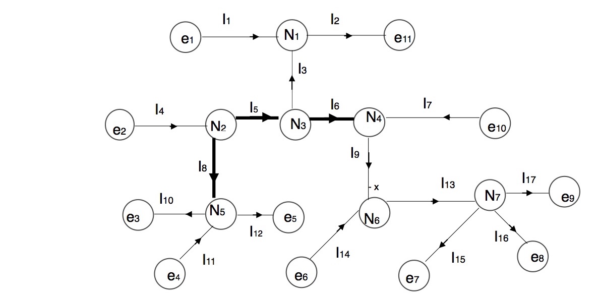
without taking into account orientations . Moreover, we call acyclic a graph which does not contain cycles: for each couple of nodes, there exists a unique path with no repeated arcs connecting them (an example of acyclic graph is in Fig. 1).

Each arc $I_{i}$ is considered as a compact one dimensional interval $[0,L_{i}]$. A function $f$ defined on $\mathcal{A}$ is a m-tuple of functions $f_{i}$, $i\in\mathcal{M}$, each one defined on $I_{i}$; $f_{i}(N_{\nu})$ denotes $f_{i}(0)$ if $N_{\nu}$ is the initial point of the arc $I_{i}$ and $f_{i}(L_{i})$ if $N_{\nu}$ is the end point, and similarly for $f(e_{j})$.

We set $\displaystyle L^{p}(\mathcal{A}):=\{f:f_{i}\in L^{p}(I_{i}),i\in{\mathcal{M}}\}$, $\displaystyle H^{s}(\mathcal{A}):=\{f:f_{i}\in H^{s}(I_{i}),i\in{\mathcal{M}}\}$ and

$$\|f\|_{2}:=\sum_{i\in{\mathcal{M}}}\|f_{i}\|_{2}\ ,\ \|f\|_{H^{s}}:=\sum_{i\in{\mathcal{M}}}\|f_{i}\|_{H^{s}}.$$

We consider the evolution of the following one-dimensional problem on the graph $\mathcal{G}$

(2.1) $$\left\{\begin{array}[]{l}\partial_{t}u_{i}+\lambda_{i}\partial_{x}v_{i}=0\ ,\\ \\ \partial_{t}v_{i}+\lambda_{i}\partial_{x}u_{i}=u_{i}\partial_{x}\phi_{i}-\beta_{i}v_{i}\ ,\qquad t\geq 0,\ x\in I_{i},\ i\in{\mathcal{M}},\\ \\ \partial_{t}\phi_{i}=D_{i}\partial_{xx}\phi_{i}+a_{i}u_{i}-b_{i}\phi_{i}\ ,\end{array}\right.$$

where $a_{i}\geq 0\ ,\lambda_{i}\ b_{i},D_{i},\beta_{i}>0$ .

We complement the system with the initial conditions

(2.2) $$u_{i0},v_{i0}\in H^{1}(I_{i})\ ,\ \phi_{i0}\in H^{2}(I_{i})\ \textrm{ for }i\in{\mathcal{M}}\ ;$$

the boundary conditions at each outer point $e_{j}$ are the null flux conditions

(2.3) $$v_{i(j)}(e_{j},t)=0\ ,\qquad\ t>0\ ,\ j\in\mathcal{J}\ ,$$
(2.4) $${\phi_{i(j)}}_{x}(e_{j},t)=0\qquad\ t>0\ ,\ j\in\mathcal{J}.$$

In addition, at each inner node $N_{\nu}$ we impose the following transmission conditions for the unknown $\phi$

(2.5) $$\left\{\begin{array}[]{ll}\displaystyle D_{i}{\phi_{i}}_{x}(N_{\nu},t)=\sum_{j\in{\mathcal{M}}^{\nu}}\alpha_{ij}^{\nu}(\phi_{j}(N_{\nu},t)-\phi_{i}(N_{\nu},t))\ \ ,\ i\in\mathcal{I}^{\nu}\ ,\ t>0\ ,\\ \\ \displaystyle-D_{i}{\phi_{i}}_{x}(N_{\nu},t)=\sum_{j\in{\mathcal{M}}^{\nu}}\alpha_{ij}^{\nu}(\phi_{j}(N_{\nu},t)-\phi_{i}(N_{\nu},t))\ ,\ \ i\in\mathcal{O}^{\nu}\ ,\ t>0\ ,\\ \\ \alpha_{ij}^{\nu}\geq 0\ ,\ \alpha_{ij}^{\nu}=\alpha_{ji}^{\nu}\ \textrm{ for all }i,j\in{\mathcal{M}}^{\nu}\ ,\end{array}\right.$$

which imply the continuity of the flux at each node, for all $t>0$,

$$\sum_{i\in\mathcal{I}^{\nu}}D_{i}{\phi_{i}}_{x}(N_{\nu},t)=\sum_{i\in\mathcal{O}^{\nu}}D_{i}{\phi_{i}}_{x}(N_{\nu},t)\ .$$

For the unknonws $v$ and $u$ we impose the transmission conditions

(2.6) $$\left\{\begin{array}[]{ll}\displaystyle-\lambda_{i}v_{i}(N_{\nu},t)=\sum_{j\in{\mathcal{M}}^{\nu}}K_{ij}^{\nu}\left(u_{j}(N_{\nu},t)-u_{i}(N_{\nu},t)\right)\ ,\ i\in\mathcal{I}^{\nu}\ ,\ t>0\ ,\\ \\ \displaystyle\lambda_{i}v_{i}(N_{\nu},t)=\sum_{j\in{\mathcal{M}}^{\nu}}K_{ij}^{\nu}\left(u_{j}(N_{\nu},t)-u_{i}(N_{\nu},t)\right)\ ,\ i\in\mathcal{O}^{\nu}\ ,\ t>0\ ,\\ \\ K_{ij}^{\nu}\geq 0\ ,\ K_{ij}^{\nu}=K_{ji}^{\nu}\ \textrm{ for all }i,j\in{\mathcal{M}}^{\nu}\ .\end{array}\right.$$

These conditions ensure the conservation of the flux of the density of cells at each node $N_{\nu}$ , for $t>0$,

$$\sum_{i\in\mathcal{I}^{\nu}}\lambda_{i}v_{i}(N_{\nu},t)=\sum_{i\in\mathcal{O}^{\nu}}\lambda_{i}v_{i}(N_{\nu},t)\ ,$$

which corresponds to the conservation of the total mass

$$\sum_{i\in{\mathcal{M}}}\int_{I_{i}}u_{i}(x,t)\ dx=\sum_{i\in{\mathcal{M}}}\int_{I_{i}}u_{0i}(x)\ dx\ ,$$

i.e. no death nor birth of individuals occours during the observation.

Motivations for the constraints on the coefficients in the transmission conditions can be found in [12] .

Finally, we impose the following compatibility conditions

(2.7) ui0,vi0,ϕi0 satisfy conditions (2.3)-(2.6) for all i.subscript𝑢𝑖0subscript𝑣𝑖0subscriptitalic-ϕ𝑖0 satisfy conditions (2.3)-(2.6) for all 𝑖u_{i0},v_{i0},\phi_{i0}\textrm{ satisfy conditions (\ref{vbc})-(\ref{TC}) for all }i\in{\mathcal{M}}\ .

Existence and uniqueness of local solutions to problem (2.1)-(2.7),

$$u,v\in C([0,T];H^{1}(\mathcal{A}))\cap C^{1}([0,T];L^{2}(\mathcal{A}))\ ,\ \phi\in C([0,T];H^{2}(\mathcal{A}))\cap C^{1}([0,T];L^{2}(\mathcal{A}))$$

are achieved in [12] by means of the linear contraction semigroup theory coupled with the abstract theory of nonhomogeneous and semilinear evolution problems; in fact, the transmission conditions (2.5) and (2.6) allows us to prove that the linear differential operators in (2.1) are m-dissipative and then, to apply the Hille-Yosida-Phillips Theorem (see [3]) . The existence of global solutions when the initial data are small in $(H^{1}(\mathcal{A}))^{2}\times H^{2}(\mathcal{A})$ norm is proved [12] too; this result holds under the further assumption

(2.8)  $$\textrm{ for all }\nu\in\mathcal{P},\textrm{ for some }k\in{\mathcal{M}}^{\nu},K_{ik}^{\nu}\neq 0\textrm{ for all }i\in{\mathcal{M}}^{\nu},i\neq k\ .$$

3. Non negative small stationary solutions on acyclic networks

In this section we approach the question of existence and uniqueness of stationary solutions of problem (2.1)-(2.8), with fixed mass

$$\mu:=\displaystyle\sum_{i\in{\mathcal{M}}}\int_{I_{i}}u_{i}(x)dx\geq 0\ ,$$

in the case of an acyclic network (see Section 2). We look for stationary solutions $(u,v,\phi)\in(H^{1}(\mathcal{A}))^{2}\times H^{2}(\mathcal{A})$.

Obviously, the flux $v$ of a stationary solution has to be constant on each arc and has to be null on the external arcs; in the case of acyclic networks, the boundary and transmission conditions (2.3), (2.6) force it to be null on each arc. In order to prove this fact we consider an internal arc $I_{j}$ and its initial node $N_{\mu}$; we consider the set

$$\mathcal{Q}=\{\nu\in\mathcal{P}:N_{\nu}\textrm{ is linked to }N_{\mu}\textrm{ by a path not covering }I_{j}\}$$

(see Fig.1: if, for example, $j=9$ then $\mu=4$, $\mathcal{Q}=\{1,2,3,5\}$ and the arcs in bold type form the path which links the nodes $N_{5}$ and $N_{4}$).

Refer to caption
Figure 1.

At each node the conservation of the flux of the density of cells, stated in Section 2, holds; then

$$\displaystyle\sum_{\nu\in\mathcal{Q}\cup\{\mu\}}\left(\sum_{i\in I^{\nu}}\lambda_{i}v_{i}(N_{\nu})-\sum_{i\in O^{\nu}}\lambda_{i}v_{i}(N_{\nu})\right)=0\ .$$

Since, for all $i\in{\mathcal{M}}$, $v_{i}(x)$ is constant on $I_{i}$ and $v_{i}(x)=0$ if $I_{i}$ is an external arc, the above equality reduces to

$$v_{j}(N_{\mu})=0\ ;$$

then $v_{j}(x)=0$ for all $x\in I_{j}$.

The previous result implies that stationary solutions must have the form $(u,0,\phi)$, where $u$ and $\phi$ have to verify the system

(3.1) $$\left\{\begin{array}[]{ll}\lambda_{i}{u_{i}}_{x}=u_{i}{\phi_{i}}_{x},\\ \\ -D_{i}{\phi_{i}}_{xx}+b_{i}\phi_{i}=a_{i}u_{i},\end{array}\right.x\in I_{i},\ i\in{\mathcal{M}},\ t>0,$$

with the boundary condition at each outer point $e_{j}$, $j\in\mathcal{J}$,

(3.2) $${\phi_{i(j)}}_{x}(e_{j},t)=0\qquad\ t>0\ ,$$

and the transmission conditions, at each inner node $N_{\nu}$,

(3.3) $$\sum_{j\in{\mathcal{M}}^{\nu}}K^{\nu}_{ij}(u_{j}(N_{\nu})-u_{i}(N_{\nu}))=0,\qquad i\in{\mathcal{M}}^{\nu}\ ,$$
(3.4) $$\begin{array}[]{ll}\displaystyle D_{i}{\phi_{i}}_{x}(N_{\nu})=\sum_{j\in{\mathcal{M}}^{\nu}}\alpha^{\nu}_{ij}(\phi_{j}(N_{\nu})-\phi_{i}(N_{\nu})),\qquad i\in\mathcal{I}^{\nu},\\ \\ \displaystyle D_{i}{\phi_{i}}_{x}(N_{\nu})=-\sum_{j\in{\mathcal{M}}^{\nu}}\alpha^{\nu}_{ij}(\phi_{j}(N_{\nu})-\phi_{i}(N_{\nu})),\qquad i\in\mathcal{O}^{\nu}.\end{array}$$

For each fixed inner node $N_{\nu}$, let $k\in\mathcal{M}^{\nu}$ be the index in condition (2.8) and let consider the transmission relations, for $i\in\mathcal{M}^{\nu}$, $i\neq k$,

(3.5) $$\begin{array}[]{ll}\displaystyle 0=\sum_{j\in{\mathcal{M}}^{\nu},j\neq i}K^{\nu}_{ij}(u_{j}(N_{\nu})-u_{i}(N_{\nu}))\\ \\ =\displaystyle\sum_{j\in{\mathcal{M}}^{\nu},j\neq i,k}K^{\nu}_{ij}(u_{j}(N_{\nu})-u_{k}(N_{\nu}))-\left(\sum_{j\in{\mathcal{M}}^{\nu},j\neq i}K^{\nu}_{ij}\right)(u_{i}(N_{\nu})-u_{k}(N_{\nu}))\ ;\end{array}$$

the assumptions on $K^{\nu}_{kj}$ in (2.8) ensure that the matrix of the coefficients of this linear system in the unknowns $(u_{j}(N_{\nu})-u_{k}(N_{\nu}))$, $j\neq k$, is non singular (if $k=1$ it is immediate to check that it has strictly dominant diagonal). Then the condition (3.3) can be rewritten as

$$\displaystyle u_{j}(N_{\nu})=u_{k}(N_{\nu})\qquad\textrm{ for all }j\in{\mathcal{M}}^{\nu}.$$

Now we fix $\mu_{0}\geq 0$ and we look for stationary solutions such that

(3.6) $$\sum_{i\in{\mathcal{M}}}\int_{I_{i}}u_{i}(x)dx=\mu_{0}\ ;$$

notice that for the evolution problem, the quantity $\displaystyle\sum_{i\in{\mathcal{M}}}\int_{I_{i}}u_{i}(x,t)dx$ is preserved for all $t\geq 0$, thanks to the transmission conditions (2.6).

Integrating the first equation in (3.1) we can rewrite problem (3.1)-(3.6) as the following elliptic problem on network:

Find $C=(C_{1},C_{2},...,C_{m})$ and $\phi\in H^{2}(\mathcal{A})$ such that

(3.7) $$\left\{\begin{array}[]{ll}\displaystyle-D_{i}{\phi_{i}}_{xx}+b_{i}\phi_{i}=a_{i}u_{i}\qquad x\in I_{i}\ ,\quad i\in{\mathcal{M}}\ ,\\ \\ u_{i}(x)=C_{i}\exp\left(\frac{\phi_{i}(x)}{\lambda_{i}}\right)\qquad x\in I_{i}\ ,\quad i\in\mathcal{M},\\ \\ {\phi_{i(j)}}_{x}(e_{j})=0\ ,\qquad j\in\mathcal{J},\\ \\ \displaystyle D_{i}{\phi_{i}}_{x}(N_{\nu})=\sum_{j\in{\mathcal{M}}^{\nu}}\alpha^{\nu}_{ij}(\phi_{j}(N_{\nu})-\phi_{i}(N_{\nu}))\ ,\qquad i\in\mathcal{I}^{\nu},\quad\nu\in\mathcal{P}\ ,\\ \\ \displaystyle D_{i}{\phi_{i}}_{x}(N_{\nu})=-\sum_{j\in{\mathcal{M}}^{\nu}}\alpha^{\nu}_{ij}(\phi_{j}(N_{\nu})-\phi_{i}(N_{\nu}))\ ,\qquad i\in\mathcal{O}^{\nu},\quad\nu\in\mathcal{P}\ ,\\ \\ C_{j}\exp\left(\frac{{\phi}_{j}(N_{\nu})}{\lambda_{j}}\right)=C_{i}\exp\left(\frac{{\phi_{i}}(N_{\nu})}{\lambda_{i}}\right)\ ,\qquad i,j\in\mathcal{M}^{\nu},\quad\nu\in\mathcal{P}\ ,\\ \\ \displaystyle\sum_{i\in{\mathcal{M}}}C_{i}\int_{I_{i}}\exp\left(\frac{{\phi_{i}}(x)}{\lambda_{i}}\right)dx=\mu_{0}\ .\end{array}\right.$$

We consider the linear operator $A:D(A)\to L^{2}(\mathcal{A})$,

(3.8) D(A)={ϕH2(𝒜):(3.2),(3.4) hold },A(ϕ)={Diϕixx+biϕi}i;𝐷𝐴conditional-setitalic-ϕsuperscript𝐻2𝒜3.23.4 hold missing-subexpressionmissing-subexpressionmissing-subexpression𝐴italic-ϕsubscriptsubscript𝐷𝑖subscriptsubscriptitalic-ϕ𝑖𝑥𝑥subscript𝑏𝑖subscriptitalic-ϕ𝑖𝑖missing-subexpression\begin{array}[]{ll}D(A)=\left\{\phi\in H^{2}(\mathcal{A}):(\ref{sbc}),(\ref{stcf})\textrm{ hold }\right\}\ ,\\ \\ A(\phi)=\left\{-D_{i}{\phi_{i}}_{xx}+b_{i}\phi_{i}\right\}_{i\in{\mathcal{M}}}\ ;\end{array}

then the equation in (3.7) and the boundary and transmission conditions for $\phi$ can be written as

(3.9) $$A\phi=F(\phi,C),$$

where, for $i\in{\mathcal{M}}$, $F_{i}(\phi(x),C)=a_{i}C_{i}\exp\left(\frac{\phi_{i}(x)}{\lambda_{i}}\right)$.

We are going to prove the existence and uniqueness of solutions to the problem (3.7) by using the Banach Fixed Point Theorem; in order to do this we need some preliminary results about the linear equation

(3.10) $$A\phi=F(f,C^{f}),$$

where $f\in H^{2}(\mathcal{A})$ is a given function, $C^{f}=(C^{f}_{1},...,C^{f}_{m})$ and $C^{f}_{i}$ are non-negative given real constants.

The existence and uniqueness of the solution $\phi\in H^{2}(\mathcal{A})$ to the above problem (for a general $F\in L^{2}(\mathcal{A})$ and a general network) is showed in [12], by Lax-Milgram theorem, in the proof of Proposition 4.1; here, we need to prove some properties holding for the solution in the case of acyclic graphs, under suitable assumptions on $f$ and $C^{f}_{i}$.

The transmission conditions (2.5) imply the following equality which will be useful in the next proofs:

(3.11) $$\begin{array}[]{ll}\displaystyle\sum_{i\in{\mathcal{M}}}\int_{I_{i}}D_{i}\left(\phi_{i}(x){\phi_{i}}_{x}(x)\right)_{x}\ dx=\\ \\ \displaystyle\sum_{\nu\in\mathcal{P}}\left(\sum_{i\in I^{\nu}}D_{i}\phi_{i}(N_{\nu}){\phi_{i}}_{x}(N_{\nu})-\sum_{i\in O^{\nu}}D_{i}\phi_{i}(N_{\nu})){\phi_{i}}_{x}(N_{\nu})\right)=\\ \\ \displaystyle\sum_{\nu\in\mathcal{P}}\ \sum_{ij\in{\mathcal{M}}^{\nu}}\alpha_{ij}^{\nu}\phi_{i}(N_{\nu})(\phi_{j}(N_{\nu})-\phi_{i}(N_{\nu}))\ =\\ \\ \displaystyle-\frac{1}{2}\sum_{\nu\in\mathcal{P}}\ \sum_{ij\in\mathcal{M}^{\nu}}\alpha^{\nu}_{ij}(\phi_{j}(N_{\nu})-\phi_{i}(N_{\nu}))^{2}\ .\end{array}$$

Let $\displaystyle|\mathcal{A}|:=\sum_{i\in\mathcal{M}}|I_{i}|$ and $\|g\|_{\infty}:=\max\{\|g_{i}\|_{\infty},i\in{\mathcal{M}}\}$.

Lemma 3.1.

Let $\mathcal{G}=(\mathcal{V},\mathcal{A})$ be an acyclic network, let $f\in H^{2}(\mathcal{A})$ and let $C_{i}^{f}$ be non-negative real numbers, for $i\in{\mathcal{M}}$. Then the solution $\phi$ to problem (3.8),(3.10) is non-negative. Moreover, if

(3.12) $$\sum_{i\in{\mathcal{M}}}C_{i}^{f}\int_{I_{i}}\exp{\left(\frac{f_{i}(x)}{\lambda_{i}}\right)}dx=\mu_{0}\ ,$$

then

(3.13) $$\|\phi_{x}\|_{\infty}\leq\frac{2\max\{a_{i}\}_{i\in{\mathcal{M}}}}{\min\{D_{i}\}_{i\in{\mathcal{M}}}}\mu_{0}\\ ;$$

if (3.12) holds and

(3.14) $$\displaystyle\|f_{x}\|_{\infty}\leq\frac{2\max\{a_{i}\}_{i\in{\mathcal{M}}}}{\min\{D_{i}\}_{i\in{\mathcal{M}}}}\mu_{0}\ ,$$

then there exists a quantity $K_{\mu_{0}}=K_{\mu_{0}}(a_{i},b_{i},D_{i},\lambda_{i},|\mathcal{A}|,\mu_{0})$, depending only on the parameters appearing in brackets, infinitesimal when $\mu_{0}$ goes to zero, such that

(3.15) $$\|\phi\|_{W^{2,1}(\mathcal{A})},\|\phi\|_{H^{2}(\mathcal{A})}\leq K_{\mu_{0}}\ .$$
Proof.

Let consider a function $\Gamma\in C^{1}({\mathbb{R}})$, strictly increasing in $(0,+\infty)$, and let $\Gamma(y)=0$ for $y\leq 0$; following standard methods for the proofs of the maximum principle for elliptic equations and setting $F_{i}(x)=F_{i}(f(x),C^{f})$, we obtain

$$\sum_{i\in{\mathcal{M}}}\int_{I_{i}}\left(-D_{i}(\phi_{i_{x}}(x)\Gamma(-\phi_{i}(x)))_{x}-D_{i}\Gamma^{\prime}(-\phi_{i}(x))\phi^{2}_{i_{x}}(x)\,+\right.\qquad$$
$$\left.\qquad\qquad\qquad b_{i}\phi_{i}(x)\Gamma(-\phi_{i}(x))-F_{i}(x)\Gamma(-\phi_{i}(x))\right)\ dx=0\ .$$

As regard to the first term, we can argue as in (3.11), taking into account the properties of $\Gamma$,

(3.16) $$\begin{array}[]{ll}\displaystyle\sum_{i\in{\mathcal{M}}}\int_{I_{i}}D_{i}\left(\Gamma(-\phi_{i}){\phi_{i}}_{x}\right)_{x}=\\ \\ \displaystyle-\frac{1}{2}\sum_{\nu\in\mathcal{P}}\ \sum_{ij\in\mathcal{M}^{\nu}}\alpha^{\nu}_{ij}(\phi_{j}(N_{\nu})-\phi_{i}(N_{\nu}))(\Gamma(-\phi_{j}(N_{\nu}))-\Gamma(-\phi_{i}(N_{\nu})))\geq 0\ ;\end{array}$$

the above inequality and the non-negativity of $F_{i}$ imply that

$$\sum_{i\in{\mathcal{M}}}b_{i}\int_{I_{i}}\phi_{i}(x)\Gamma(-\phi_{i}(x))dx\geq 0\ ,$$

so that, thanks to the properties of $\Gamma$ , we can conclude that $\phi_{i}(x)\geq 0$ for all $i\in{\mathcal{M}}$.

By integration of the equation (3.10), taking into account (3.4) and (3.2), we obtain

(3.17) $$\sum_{i\in{\mathcal{M}}}b_{i}\int_{I_{i}}\phi_{i}(x)dx=\sum_{i\in{\mathcal{M}}}\int_{I_{i}}F_{i}(f(x),C^{f})dx$$

which implies

(3.18) $$\|\phi\|_{1}\leq K_{1}(a_{i},b_{i})\mu_{0}\ .$$

In order to obtain (3.13), first we notice that, if $I_{j}$ is an external arc, then the following inequality holds

$$|D_{j}{\phi_{j}}_{x}(x)|\leq\int_{I_{j}}D_{j}|{\phi_{j}}_{yy}(y)|\ dy\leq\int_{I_{j}}\left(b_{j}\phi_{j}(y)+C_{j}^{f}a_{j}\exp\left(\frac{f_{j}(y)}{\lambda_{j}}\right)\right)dy\ .$$

Then we consider an internal arc $I_{j}$ and its initial node $N_{\mu}$ and the sets

$$\mathcal{Q}=\{\nu\in\mathcal{P}:N_{\nu}\textrm{ is linked to }N_{\mu}\textrm{ by a path not covering }I_{j}\}\ ,$$
$$\mathcal{S}=\{i\in\mathcal{M}:I_{i}\textrm{ is incident with }N_{l}\textrm{ for some }l\in\mathcal{Q}\}$$

(see Fig.1: if, for example, $j=9$, then $\mu=4$, $\mathcal{Q}=\{1,2,3,5\}$, $\mathcal{S}=\{1,2,3,4,5,6,8,$ $10,11,12\}$); at each node the conservation of the flux, stated in Section 2 as a consequence of the transmission conditions, holds; then

$$\displaystyle\sum_{\nu\in\mathcal{Q}\cup\{\mu\}}\left(\sum_{i\in I^{\nu}}D_{i}{\phi_{i}}_{x}(N_{\nu})-\sum_{i\in O^{\nu}}D_{i}{\phi_{i}}_{x}(N_{\nu})\right)=0\ .$$

Let $x$ be a point on the arc $I_{j}$ (see Fig.1 for $j=9$, $\mu=4$) and $I_{j}^{x}$ the part of $I_{j}$ which connects $N_{\mu}$ and $x$; then, using the above equality and the boundary conditions (2.4), we have

$$|D_{j}{\phi_{j}}_{x}(x)|=\left|D_{j}{\phi_{j}}_{x}(x)+\displaystyle\sum_{\nu\in\mathcal{Q}\cup\{\mu\}}\left(\sum_{i\in I^{\nu}}D_{i}{\phi_{i}}_{x}(N_{\nu})-\sum_{i\in O^{\nu}}D_{i}{\phi_{i}}_{x}(N_{\nu})\right)\right|=$$
$$\left|\sum_{i\in\mathcal{S}}\int_{I_{i}}D_{i}{\phi_{i}}_{yy}(y)\ dy+\int_{I_{j}^{x}}D_{j}{\phi_{j}}_{yy}(y)\ dy\right|=$$
$$\left|\sum_{i\in\mathcal{S}}\int_{I_{i}}\left(b_{i}\phi_{i}(y)-C_{i}^{f}a_{i}\exp\left(\frac{f_{i}(y)}{\lambda_{i}}\right)\right)dy+\int_{I_{j}^{x}}\left(b_{j}\phi_{j}(y)-C_{j}^{f}a_{j}\exp\left(\frac{f_{j}(y)}{\lambda_{j}}\right)\right)dy\right|\ .$$

Then $\displaystyle D_{j}\|\phi_{j_{x}}\|_{\infty}\leq 2\mu_{0}\max\{a_{i}\}_{i\in{\mathcal{M}}}$ for all $j\in{\mathcal{M}}$ and we obtain (3.13) which implies

(3.19) $$\|\phi_{x}\|_{1}\leq\frac{2\max\{a_{i}\}_{i\in{\mathcal{M}}}}{\min\{D_{i}\}_{i\in{\mathcal{M}}}}|\mathcal{A}|\mu_{0}\,,$$

and

(3.20) $$\|\phi_{x}\|_{2}\leq\frac{2\max\{a_{i}\}_{i\in{\mathcal{M}}}}{\min\{D_{i}\}_{i\in{\mathcal{M}}}}|\mathcal{A}|^{\frac{1}{2}}\mu_{0}\ ;$$

moreover, by Sobolev embedding theorem, we obtain

$$\|\phi\|_{\infty}\leq K_{4}(a_{i},b_{i},D_{i},|\mathcal{A}|)\mu_{0}\ ,$$

where $K_{4}$ is a suitable constant.

The estimates for the function $\phi_{xx}$ follow by using the equation (3.10), taking into account (3.12), (3.14). In particular, from the equation (3.10), using (3.11), we have

$$\sum_{i\in{\mathcal{M}}}\frac{D_{i}^{2}}{b_{i}}\int_{I_{i}}{\phi_{i}}_{xx}^{2}(x)\ dx\leq\sum_{i\in{\mathcal{M}}}\frac{\|F_{i}\|_{\infty}}{b_{i}}\int_{I_{i}}F_{i}(x)\ dx\leq\frac{\max\{a_{i}\|F_{i}\|_{\infty}\}}{\min\{b_{i}\}}\mu_{0}$$

and the embedding of $W^{1,1}(I_{i})$ in $L^{\infty}(I_{i})$ gives

$$\sum_{i\in{\mathcal{M}}}\frac{D_{i}^{2}}{b_{i}}\int_{I_{i}}{\phi_{i}}_{xx}^{2}(x)\ dx\leq K_{5}(1+\|{f}_{x}\|_{\infty})\mu_{0}^{2}$$

where $K_{5}=K_{5}(a_{i},b_{i},D_{i},\lambda_{i})$ . ∎

Now we can prove the following theorem.

Theorem 3.1.

Let $\mathcal{G}=(\mathcal{V},\mathcal{A})$ be an acyclic network. There exists $\epsilon>0$ such that, if $0\leq\mu_{0}\leq\epsilon$ , then problem (2.1)-(2.8) has a unique stationary solution satisfying (3.6); the solution has the form

$$\left(C_{i}\exp\left(\frac{{\phi_{i}}(x)}{\lambda_{i}}\right),0,\phi_{i}(x)\right)\ \ i\in{\mathcal{M}},$$

where $\phi_{i}(x)\geq 0$ and $C_{i}$ are nonnegative constants such that $u_{j}(N_{\nu})=u_{i}(N_{\nu})$ for all $\nu\in\mathcal{P}$, $i,j\in\mathcal{M}^{\nu}$.

Proof.

First we notice that, if a stationary solution $(u,v,\phi)$ satisfying (3.6) exists, then $u$ is non-negative, since the costants $C_{i}$ in (3.7) must have the same sign, so that they have to be non-negative to satisfy the condition $\mu_{0}\geq 0$; arguing as in the proof of Lemma 3.1 we prove that $\phi$ is non-negative too. If $\mu_{0}>0$ then $u$ and $\phi$ are positive functions.

We are going to use a fixed point technique. Given $\phi^{0}\in D(A)$, we want to define a function $u^{0}(x)$ on the network, such that, for $i\in{\mathcal{M}}$,

$$u_{i}^{0}(x)=C^{\phi^{0}}_{i}\exp\left(\frac{\phi_{i}^{0}(x)}{\lambda_{i}}\right)\,,$$

where the constants $C_{i}^{\phi^{0}}$ satisfy the following linear system composed by the last conditions in (3.7)

(3.21) $$\displaystyle C^{\phi^{0}}_{j}\exp\left(\frac{\phi^{0}_{j}(N_{\nu})}{\lambda_{j}}\right)=C^{\phi^{0}}_{i}\exp\left(\frac{{\phi_{i}}^{0}(N_{\nu})}{\lambda_{i}}\right)\ ,\qquad i,j\in\mathcal{M}^{\nu},\quad\nu\in\mathcal{P}\ ,$$
(3.22) $$\displaystyle\sum_{i\in{\mathcal{M}}}C^{\phi^{0}}_{i}\int_{I_{i}}\exp\left(\frac{{\phi_{i}}^{0}(x)}{\lambda_{i}}\right)dx=\mu_{0}\ .$$

The system (3.21),(3.22) has a unique solution; actually, since the network has no cycles, the system (3.21) has $\infty^{1}$ solutions $C^{\phi^{0},\alpha}=(\alpha,\alpha\delta_{2},\alpha\delta_{3},...,\alpha\delta_{m})$, $\alpha\in{\mathbb{R}}$, where $\delta_{i}$ are suitable coefficients, and the condition (3.22) determines the value of $\alpha$.

In order to give an explicit expression for the coefficients $\delta_{i}$ we consider an arc, $I_{1}$, and we define

$$u^{0}_{1}(x):=\alpha\exp\left(\frac{\phi_{1}^{0}(x)}{\lambda_{1}}\right)\ .$$

Let $N_{\mu}$ one of the extreme points of $I_{1}$, then we define the function $u^{0}$ on the other arcs which are incident with $N_{\mu}$ in such a way to verify the equalities in (3.21) for the node $N_{\mu}$,

$$u^{0}_{j}(x):=\alpha\exp\left(\frac{\phi_{1}^{0}(N_{\mu})}{\lambda_{1}}\right)\exp\left(-\frac{\phi_{j}^{0}(N_{\mu})}{\lambda_{j}}\right)\exp\left(\frac{\phi_{j}^{0}(x)}{\lambda_{j}}\right)\ \textrm{ for all }j\in\mathcal{M}^{\mu}\,,j\neq 1;$$

i.e. we set $C^{\phi^{0}}_{j}=\alpha\exp\left(\frac{\phi_{1}^{0}(N_{\mu})}{\lambda_{1}}\right)\exp\left(-\frac{\phi_{j}^{0}(N_{\mu})}{\lambda_{j}}\right)$ , $j\in\mathcal{M}^{\mu}\,,j\neq 1$.

Refer to caption
Figure 2.

This procedure can be iterated at each node reached by one of the arcs $I_{j}$, $j\in{\mathcal{M}}^{\mu}$, and at the other extreme point of $I_{1}$, if it is an internal arc, and so on, defining in this way the function $u^{0}$ on each arc of the network. Notice that this construction is possible since there are no cycles in the graph. The function $u$ can be expressed, on each arc of the network, as follows (if it is the case, renumbering in suitable way the arcs and the nodes): let consider the path from the outer point $e_{1}$ to an inner node $N_{h-1}$, composed from the arcs $I_{i}$, $i=1,...,h-1$, (passing through the vertexes $N_{i}$, $i=1,...,h-1$), and let $I_{h}$ be an arc incident with the node $N_{h-1}$, not belonging to the path (see Fig.2 where h=5 and the highlighted arcs forms the path); following the procedure described before, after setting

$$\displaystyle\mathcal{E}_{h}(\phi^{0}):=\frac{\Pi_{i=1,...,h-1}\exp\left(\frac{\phi^{0}_{i}(N_{i})}{\lambda_{i}}\right)}{\Pi_{i=1,...,h-1}\exp\left(\frac{\phi^{0}_{i+1}(N_{i})}{\lambda_{i+1}}\right)}\ ,$$

we define

$$u^{0}_{h}(x):=\alpha\mathcal{E}_{h}(\phi^{0})\exp\left(\frac{\phi^{0}_{h}(x)}{\lambda_{h}}\right)\ .$$

The quantity $\alpha$ is fixed in such a way to verify the last condition in (3.7),

$$\alpha\sum_{i\in{\mathcal{M}}}\mathcal{E}_{i}(\phi^{0})\int_{I_{i}}\exp\left(\frac{{\phi_{i}}^{0}(x)}{\lambda_{i}}\right)dx=\mu_{0}\ ,$$

so that, for all $i\in{\mathcal{M}}$,

(3.23) $$u^{0}_{i}(x)=\displaystyle C_{i}^{\phi^{0}}\exp\left(\frac{\phi_{i}^{0}(x)}{\lambda_{i}}\right)\ ,\ \ C_{i}^{\phi^{0}}:=\mu_{0}\frac{\ \mathcal{E}_{i}(\phi^{0})}{\displaystyle\ \sum_{j\in{\mathcal{M}}}\mathcal{E}_{j}(\phi^{0})\int_{I_{j}}\exp\left(\frac{{\phi}^{0}_{j}(x)}{\lambda_{j}}\right)dx\ }.$$

Let $G$ be the operator defined in $D(A)$ such that $\phi^{1}:=G(\phi^{0})$ is the solution of problem (3.10) where $f=\phi_{0}$ and $C_{i}^{f}=C_{i}^{\phi^{0}}$ for $i\in{\mathcal{M}}$,

$$A\phi^{1}=F(C^{\phi^{0}},\phi^{0})\ ;$$

let $K_{\mu_{0}}=K_{\mu_{0}}(a_{i},b_{i},D_{i},\lambda_{i},|\mathcal{A}|,{\mu_{0}})$ be the quantity in Lemma 3.1, and let

$$B_{\mu_{0}}:=\{\phi\in D(A):\phi\geq 0\ ,\|\phi_{x}\|_{\infty}\leq\frac{2\max\{a_{i}\}_{i\in{\mathcal{M}}}}{\min\{D_{i}\}_{i\in{\mathcal{M}}}}\mu_{0}\ ,\|\phi\|_{H^{2}}\leq K_{\mu_{0}}\ \}$$

equipped with the distance $d$ generated by norm of $H^{2}(\mathcal{A})$; $(B_{\mu_{0}},d)$ is a complete metric space. From the lemma we know that solutions to problem (3.8)-(3.12) have to belong to $B_{\mu_{0}}$, then $G(B_{\mu_{0}})\subseteq B_{\mu_{0}}$; next we are proving that, if $\mu_{0}$ is small enough, then $G$ is a contraction in $B_{\mu_{0}}$.

We consider $\phi^{0},\overline{\phi}^{0}\in B_{\mu_{0}}$ and the corresponding $u^{0},\overline{u}^{0}$ and $\phi^{1},\overline{\phi}^{1}$; using the equation satisfied by $\phi^{0}$ and $\overline{\phi}^{0}$ , for all $i\in{\mathcal{M}}$ we can write

(3.24) $$\begin{array}[]{ll}\displaystyle b_{i}\int_{I_{i}}(\phi^{1}_{i}(x)-\overline{\phi}^{1}_{i}(x))^{2}\,dx+D_{i}\int_{I_{i}}(\phi^{1}_{ix}(x)-\overline{\phi}^{1}_{ix}(x))^{2}\,dx\\ \\ \displaystyle-D_{i}\int_{I_{i}}\left((\phi^{1}_{ix}(x)-\overline{\phi}^{1}_{ix}(x))(\phi^{1}_{i}(x)-\overline{\phi}^{1}_{i}(x))\right)_{x}\,dx\\ \\ \displaystyle=a_{i}\int_{I_{i}}(u^{0}_{i}(x)-\overline{u}^{0}_{i}(x))(\phi^{1}_{i}(x)-\overline{\phi}^{1}_{i}(x))\ \,dx\ ;\end{array}$$

using (3.11), from (3.24) we infer that

(3.25) $$\sum_{i\in{\mathcal{M}}}\|{\phi_{i}}^{1}-\overline{\phi_{i}}^{1}\|_{H^{2}}\leq K(a_{i},b_{i},D_{i})\sum_{i\in{\mathcal{M}}}\|u^{0}_{i}-\overline{u}_{i}^{0}\|_{2}\ ,$$

We set

$$J_{i}^{\phi^{0}}:=\int_{I_{i}}\exp\left(\frac{{\phi_{i}}^{0}(x)}{\lambda_{i}}\right)dx\,,\qquad E_{i}^{\phi^{0}}(x):=\exp\left(\frac{{\phi_{i}}^{0}(x)}{\lambda_{i}}\right)\ \ ;$$

we have

(3.26) $$\begin{array}[]{ll}\displaystyle|u_{i}^{0}(x)-\overline{u}_{i}^{0}(x)|=\displaystyle\mu_{0}\left|\frac{\ \mathcal{E}_{i}(\phi^{0})E^{\phi^{0}}_{i}(x)\ }{\displaystyle\ \sum_{j\in{\mathcal{M}}}\mathcal{E}_{j}(\phi^{0})J_{j}^{\phi^{0}}\ }-\frac{\ \mathcal{E}_{i}(\overline{\phi}^{0})E^{\overline{\phi}^{0}}_{i}(x)\ }{\ \displaystyle\sum_{j\in{\mathcal{M}}}\mathcal{E}_{j}(\overline{\phi}^{0})J^{\overline{\phi}^{0}}_{j}\ }\right|\par\par\par\ .\end{array}$$

In order to treat the above quantity we have to consider that, for all $g\in B_{\mu_{0}}$, $E^{g}_{i}(x)\geq 1$, ${J^{g}_{i}}\geq|I_{i}|$ and there exists a constant $K_{6}=K_{6}(K_{\mu_{0}},\lambda_{i})$, increasing with $\mu_{0}$, such that, for all $i\in{\mathcal{M}}$

$$\max_{I_{i}}E^{g}_{i}(x)\leq K_{6}\ ,\quad J_{i}^{g}\leq K_{6}|I_{i}|\ ,$$
$$\left|E^{\phi^{0}}_{i}(x)-{E^{\overline{\phi}^{0}}_{i}}(x)\right|\leq K_{6}|\phi_{i}^{0}(x)-\overline{\phi}_{i}^{0}(x)|\ ,$$
$$|J_{i}^{\phi^{0}}-J_{i}^{\overline{\phi}^{0}}|\leq K_{6}\int_{I_{i}}|\phi_{i}^{0}(x)-\overline{\phi}_{i}^{0}(x)|\,dx\ .$$

The above inequalities can be used in (3.26) so that (3.25) implies

(3.27) $$\sum_{i\in{\mathcal{M}}}\|{\phi_{i}}^{1}-\overline{\phi_{i}}^{1}\|_{H^{2}}\leq\mu_{0}K_{7}(a_{i},b_{i},D_{i},K_{\mu_{0}},|\mathcal{A}|)\sum_{i\in{\mathcal{M}}}\|\phi_{i}^{0}-\overline{\phi}_{i}^{0}\|_{H^{1}}\ ,$$

where $K_{7}$ increases with $\mu_{0}$; hence, for $\mu_{0}$ small enough, $G$ is a contraction on $B_{\mu_{0}}$ and we can use the Banach Fixed Point Theorem.

Let $\phi$ be the unique fixed point of $G$ in $B_{\mu_{0}}$ and let $C^{\phi}=(C_{1}^{\phi},C_{2}^{\phi},...,C_{m}^{\phi})$ where $C_{i}^{\phi}$, for $i\in{\mathcal{M}}$, are computed as in (3.23); then $(\phi,C^{\phi})$ is the unique solution to Problem (3.7)3.7(\ref{pr-ell2}) and the claim is proved.

For any constant $U\geq 0$, the triple $(U,0,\frac{a_{i}}{b_{i}}U)$ satisfies the equations in (2.1) on the arc $I_{i}$. Let $Q$ be a real non-negative number; if $\frac{a_{i}}{b_{i}}=Q$ for all $i\in{\mathcal{M}}$, then the same triple $(U,0,QU)$ satisfies the equations on each arc $I_{i}$ and it is a stationary solution to the problem (2.1)-(2.8). Then, as a consequence of the previous theorem, we have the following proposition, with $\epsilon$ as in the theorem.

Proposition 3.1.

Let $\mathcal{G}=(\mathcal{V},\mathcal{A})$ be an acyclic network. If $\frac{a_{i}}{b_{i}}=Q$ for all $i\in{\mathcal{M}}$ and $0\leq\mu_{0}\leq\epsilon$, then the unique stationary solution to problem (2.1)-(2.8), (3.6) is the constant solution $\displaystyle\left(\frac{\mu_{0}}{|\mathcal{A}|},0,Q\frac{\mu_{0}}{|\mathcal{A}|}\right)$.

Remark 3.1 For general networks, when the value of $\frac{a_{i}}{b_{i}}=Q$ on each arc, the stationary solution of Proposition 3.1 always exists. More precisely, if $\frac{a_{i}}{b_{i}}=Q$, in the class of the functions $(u,v,\phi)$ which are constant on each arc, the stationary solution $\displaystyle\left(\frac{\mu_{0}}{|\mathcal{A}|},0,Q\frac{\mu_{0}}{|\mathcal{A}|}\right)$ is the unique stationary solution with mass $\mu_{0}$; this fact is true without any restrictions on the value of $\mu_{0}$ and on the structure of the network. Actually, if we assume that $u$ is constant on each arc, then, using the equations, we infer that, on each arc, $\phi_{x}(x)$ is constant too, hence $\phi_{xx}=0$ and $\phi(x)$ is constant. Then $v(x)=0$ on each arc; hence, arguing as at the beginning of this section, we obtain that $u$ is continuous on the network.

In the next proposition we are going to prove that, in a set of small solutions, such stationary solution is the unique one with fixed mass $\mu_{0}$.

Proposition 3.2.

Let $\frac{a_{i}}{b_{i}}=Q$ for all $i\in{\mathcal{M}}$ and let $(u,v,\phi)\in(H^{1}(\mathcal{A}))^{2}\times H^{2}(\mathcal{A})$ be a stationary solution of problem (2.1)-(2.8),(3.6). There exists $\epsilon_{0}>0,$ depending on $\lambda_{i},a_{i},b_{i},D_{i},\beta_{i},|\mathcal{A}|$, such that, if $\|u\|_{H^{1}}\leq\epsilon_{0}$, then $(u,v,\phi)=\displaystyle\left(\frac{\mu_{0}}{|\mathcal{A}|},0,Q\frac{\mu_{0}}{|\mathcal{A}|}\right)$.

Proof.

We set $H:=\|u\|_{H^{1}}$. The transmission conditions (2.6) imply that

$$\sum_{\nu\in\mathcal{P}}\left(\sum_{i\in\mathcal{I}^{\nu}}\lambda_{i}u_{i}(N^{\nu})v_{i}(N^{\nu})-\sum_{i\in\mathcal{O}^{\nu}}\lambda_{i}u_{i}(N^{\nu})v_{i}(N^{\nu})\right)\geq 0\ ,$$

so, by using the first two equations in (2.1), we obtain

$$2\sum_{i\in{\mathcal{M}}}\beta_{i}\int_{I_{i}}v_{i}^{2}(x)dx\leq\sum_{i\in{\mathcal{M}}}\|u_{i}\|_{\infty}\int_{I_{i}}(v_{i}^{2}(x)+\phi^{2}_{i_{x}}(x))\ dx\ ,$$
$$\sum_{i\in{\mathcal{M}}}\lambda_{i}\int_{I_{i}}u^{2}_{i_{x}}(x)\ dx\leq\sum_{i\in{\mathcal{M}}}\|u_{i}\|_{\infty}\int_{I_{i}}(u_{i_{x}}^{2}(x)+\phi^{2}_{i_{x}}(x))\ dx\ +\qquad\qquad\qquad$$
$$\qquad\sum_{i\in{\mathcal{M}}}\frac{\beta_{i}^{2}}{\lambda_{i}}\int_{I_{i}}v^{2}_{i}(x)\ dx\ ;$$

the above inequalities implies the following one

(3.28) $$\|v\|_{2}^{2}+\|u_{x}\|_{2}^{2}\leq K_{0}H\left(\|\phi_{x}\|_{2}^{2}+\|v\|_{2}^{2}+\|u_{x}\|_{2}^{2}\right)\ ,$$

where $K_{0}$ is a positive constant depending on the parameters $\lambda_{i},\beta_{i}$ and the Sobolev embedding costant.

The transmission conditions (2.5) imply that

$$-\sum_{\nu\in\mathcal{P}}\left(\sum_{i\in\mathcal{I}^{\nu}}D_{i}\phi_{i}(N^{\nu}){\phi_{i}}_{x}(N^{\nu})-\sum_{i\in\mathcal{O}^{\nu}}D_{i}\phi_{i}(N^{\nu}){\phi_{i}}_{x}(N^{\nu})\right)\geq 0\ ;$$

moreover, the assumption (2.8) imply that, for each $\nu\in\mathcal{P}$, for suitable coefficients $\theta^{\nu}_{ij}$ and suitable $k\in{\mathcal{M}}^{\nu}$,

$$\displaystyle u_{j}(N_{\nu})=u_{k}(N_{\nu})+\sum_{i\in{\mathcal{M}}^{\nu},i\neq k}\theta^{\nu}_{ij}v_{i}(N_{\nu})\qquad\textrm{ for all }j\in{\mathcal{M}}^{\nu}\ ,$$

(see Lemma 5.9 in [12]); then, by the last equation in (2.1), arguing as in the proof of Proposition 5.8 in [12], we obtain

(3.29) $$\|\phi_{x}\|_{2}^{2}+\|\phi_{xx}\|_{2}^{2}\leq K_{1}\left(\|v\|_{2}^{2}+\|u_{x}\|_{2}^{2}\right)\ ,$$

where $K_{1}$ is a positive constant depending on the parameters $D_{i},a_{i},b_{i},\theta^{\nu}_{ij}$.

By inequalities (3.28) and (3.29) we deduce the following one

$$\|v\|_{2}^{2}+\|u_{x}\|_{2}^{2}\leq K_{0}(1+K_{1})H\left(\|v\|_{2}^{2}+\|u_{x}\|_{2}^{2}\right)\ ,$$

which, for small $H$, implies $\|v\|_{2},\|u_{x}\|_{2}=0$.

In the cases when $\frac{a_{i}}{b_{i}}$ depends on the arc in consideration, stationary solutions with the component $u$ constant on each arc, can be inadmissible. As we showed before, $v$ should be zero, $u$ should be constant on the whole network and $\phi$ should be constant on each arc,

$$u_{i}(x)=\frac{\mu_{0}}{|\mathcal{A}|}\ ,\ \ \ \phi_{i}(x)=\frac{a_{i}}{b_{i}}\frac{\mu_{0}}{|\mathcal{A}|}\ ,\qquad i\in{\mathcal{M}}\ .$$

Therefore the transmission conditions, for each $\nu\in\mathcal{P}$,

$$\sum_{j\in{\mathcal{M}}^{\nu}}\alpha^{\nu}_{ij}\frac{\mu_{0}}{|\mathcal{A}|}\left(\frac{a_{j}}{b_{j}}-\frac{a_{i}}{b_{i}}\right)=0\ ,\qquad i\in{\mathcal{M}}^{\nu}\ ,$$

are constraints on the relations between the parameters of the problem which have to hold if the constant stationary solution exists.

For example, in the case of two arcs, if $\frac{b_{2}}{a_{2}}\neq\frac{b_{1}}{a_{1}}$ (and $0<\mu_{0}\leq\epsilon$), the stationary solution can not be constant on the arcs , since the trasmission condition at the node,

$$\alpha_{11}\frac{\mu_{0}}{|\mathcal{A}|}\left(\frac{b_{2}}{a_{2}}-\frac{b_{1}}{a_{1}}\right)=0\ ,$$

cannot be satisfied.

Hence, in the cases when $\frac{a_{i}}{b_{i}}$ depends on the arc in consideration, if $(u,v,\phi)$ is the stationary solution in Theorem 3.1, then $u$ is a continuous function on all the network but it is not constant on each arc.

4. Asymptotic behaviour

In this section we are going to show that the constant stationary solutions previously introduced, provide the asymptotic profiles for a class of solutions to problem (2.1)-(2.8). We recall that existence and uniqueness of global solutions

(4.1) $$\begin{array}[]{ll}u,v\in C\left([0,+\infty);H^{1}(\mathcal{A})\right)\cap C^{1}\left([0,+\infty);L^{2}(\mathcal{A})\right),\\ \\ \phi\in C\left([0,+\infty);H^{2}(\mathcal{A})\right)\cap C^{1}\left([0,+\infty);L^{2}(\mathcal{A})\right),\par\phi_{x}\in H^{1}\left((0,+\infty)\times\mathcal{A}\right),\end{array}$$

to such problem is proved in [12], when the initial data are sufficiently small in $(H^{1}(\mathcal{A}))^{2}\times H^{2}(\mathcal{A})$ norm and the following condition holds

(4.2) $$\frac{a_{i}}{b_{i}}=Q\ \ \textrm{for all }i\in{\mathcal{M}}\ ;$$

in particular it is proved that the functional $F$ defined by

(4.3) $$\begin{array}[]{ll}\displaystyle F_{T}^{2}(u,v,\phi):=\sum_{i\in{\mathcal{M}}}\left(\sup_{t\in[0,T]}\|u_{i}(t)\|_{H^{1}}^{2}+\sup_{t\in[0,T]}\|v_{i}(t)\|_{H^{1}}^{2}+\sup_{t\in[0,T]}\|{\phi_{i}}_{x}(t)\|_{H^{1}}^{2}\right)\\ \\ \displaystyle+\int_{0}^{T}\left(\|u_{x}(t)\|_{2}^{2}+\|v(t)\|_{H^{1}}^{2}+\|v_{t}(t)\|_{2}^{2}+\|\phi_{x}(t)\|_{H^{1}}^{2}+\|\phi_{xt}(t)\|_{2}^{2}\right)\ dt\end{array}$$

is uniformly bounded for $T>0$.

Here and below we use the notations

$$\|f_{i}(t)\|_{2}:=\|f_{i}(\cdot,t)\|_{L^{2}(I_{i})},\ \ \|f_{i}(t)\|_{H^{s}}:=\|f_{i}(\cdot,t)\|_{H^{s}(I_{i})}\ .$$

Now we assume (4.2), we fix $\overline{\mu}\geq 0$ and we consider the constant stationary solution, $(\overline{u},0,\overline{\phi})$, to problem (2.1)-(2.8), such that $\displaystyle\overline{u}|\mathcal{A}|=\overline{\mu}$; moreover let $(\tilde{u}_{0},\tilde{v}_{0},\tilde{\phi}_{0})\in(H^{1}(\mathcal{A}))^{2}\times H^{2}(\mathcal{A})$ be a small perturbation of $(\overline{u},0,\overline{\phi})$, i.e., setting $u_{0}:=\tilde{u}_{0}-\overline{u},v_{0}:=\tilde{v}_{0},\phi_{0}:=\tilde{\phi}_{0}-\overline{\phi}$ , the $(H^{1}(\mathcal{A}))^{2}\times H^{2}(\mathcal{A})$ norm of $(u_{0},v_{0},\phi_{0})$ is bounded by a suitable small $\epsilon_{0}>0$.

If $(\tilde{u},\tilde{v},\tilde{\phi})$ is the solution to problem (2.1)-(2.8) with initial data $(\tilde{u}_{0},\tilde{v}_{0},\tilde{\phi}_{0})$ and $u:=\tilde{u}-\overline{u},v:=\tilde{v},\phi:=\tilde{\phi}-\overline{\phi}$ , then $(u,v,\phi)$ is solution to the system

(4.4) $$\left\{\begin{array}[]{l}\partial_{t}u_{i}+\lambda_{i}\partial_{x}v_{i}=0\\ \\ \partial_{t}v_{i}+\lambda_{i}\partial_{x}u_{i}=(u_{i}+\overline{u})\partial_{x}\phi_{i}-\beta_{i}v_{i}\qquad\qquad x\in I_{i}\,,t\geq 0\,,i\in{\mathcal{M}},\\ \\ \partial_{t}\phi_{i}=D_{i}\partial_{xx}\phi_{i}+a_{i}u_{i}-b_{i}\phi_{i}\ ,\end{array}\right.$$

complemented with the conditions (2.2)-(2.8) and initial data $(u_{0},v_{0},\phi_{0})$ defined above.

The existence and uniqueness of local solutions to this problem can be achieved by means of semigroup theory, following the method used in[12], with little modifications.

On the other hand, if we assume that $\overline{u}$ is suitably small, the method used in that paper to obtain the global existence result in the case of small initial data can be used here too, modifying the estimates in order to treat the further term in the second equation and then using the smallness of $\overline{u}$.

Below we list a priori estimates holding for the solutions to problem (4.4), (2.2)-(2.7); we don’t give the proofs since they are equal to those in [12], in Section 5, except for easy added calculations to treat the term $\overline{u}{\phi_{i}}_{x}$.

Proposition 4.1.

Let $(u,v,\phi)$ be a local solution to problem (4.4),(2.2)-(2.7),

$$\begin{array}[]{ll}u,v\in C\left([0,T];H^{1}(\mathcal{A})\right)\cap C^{1}\left([0,T];L^{2}(\mathcal{A})\right)\ ,\\ \\ \phi\in C\left([0,T];H^{2}(\mathcal{A})\right)\cap C^{1}\left([0,T];L^{2}(\mathcal{A})\right)\ ,\ \phi_{x}\in H^{1}\left((0,T)\times\mathcal{A}\right)\ ;\end{array}$$

then

  • a)
    $$\begin{array}[]{ll}\displaystyle\sum_{i\in{\mathcal{M}}}\left(\sup_{[0,T]}\|u_{i}(t)\|_{2}^{2}+\sup_{[0,T]}\|v_{i}(t)\|_{2}^{2}+\beta_{i}\int_{0}^{T}\|v_{i}(t)\|_{2}^{2}dt\right)\\ \\ \leq C\displaystyle\sum_{i\in{\mathcal{M}}}\left(\|u_{0i}\|_{2}^{2}+\|v_{0i}\|_{2}^{2}\right)\\ \\ +\displaystyle C\sum_{i\in{\mathcal{M}}}\left(\sup_{[0,T]}\|u_{i}(t)\|_{H^{1}}+\overline{u}\right)\int_{0}^{T}\left(\|{\phi_{i}}_{x}(t)\|_{2}^{2}+\|v_{i}(t)\|_{2}^{2}\right)dt\ ;\end{array}$$
  • b)
    $$\begin{array}[]{ll}\displaystyle\sum_{i\in{\mathcal{M}}}\left(\sup_{[0,T]}\|{v_{i}}_{x}(t)\|_{2}^{2}+\sup_{[0,T]}\|{v_{i}}_{t}(t)\|_{2}^{2}+\int_{0}^{T}\|{v_{i}}_{t}(t)\|_{2}^{2}\,dt\right)\\ \\ \leq\displaystyle C\left(\|v_{0}\|_{H^{1}}^{2}+\|u_{0}\|_{H^{1}}^{2}\|\phi_{0}\|_{H^{2}}^{2}\right)\\ \\ +\displaystyle C\sum_{i\in{\mathcal{M}}}\left(\sup_{[0,T]}\|u_{i}(t)\|_{H^{1}}+\overline{u}\right)\int_{0}^{T}\left({\phi_{i}}_{xt}(t)\|_{2}^{2}+\|{v_{i}}_{t}(t)\|_{2}^{2}\right)\ dt\\ \\ +\displaystyle C\sum_{i\in{\mathcal{M}}}\sup_{[0,T]}\|\phi_{x}(t)\|_{H^{1}}\int_{0}^{T}\left(\|{v_{i}}_{t}(t)\|_{2}^{2}+\|v_{i}(t)\|_{H^{1}}^{2}\right)\,dt\ ;\end{array}$$
  • c)
    $$\begin{array}[]{ll}\displaystyle\sum_{i\in{\mathcal{M}}}\sup_{[0,T]}\|{u_{i}}_{x}(t)\|_{2}^{2}\leq C\sum_{i\in{\mathcal{M}}}\left(\sup_{[0,T]}\|{v_{i}}_{t}(t)\|_{2}^{2}+\sup_{[0,T]}\|v_{i}(t)\|_{2}^{2}\right)\\ \\ \displaystyle+C\sum_{i\in{\mathcal{M}}}\left(\sup_{[0,T]}\|u_{i}(t)\|_{H^{1}}+\overline{u}\right)\left(\sup_{[0,T]}\|{u_{i}}_{x}(t)\|_{2}^{2}+\sup_{[0,T]}\|{\phi_{i}}_{x}(t)\|_{2}^{2}\right)\ ;\end{array}$$
  • d)
    $$\begin{array}[]{ll}\displaystyle\sum_{i\in{\mathcal{M}}}\int_{0}^{T}\|{u_{i}}_{x}(t)\|_{2}^{2}\,dt\leq C\sum_{i\in{\mathcal{M}}}\int_{0}^{T}\left(\|{v_{i}}_{t}(t)\|_{2}^{2}+\|v_{i}(t)\|_{2}^{2}\right)\,dt\\ \\ \displaystyle+C\sum_{i\in{\mathcal{M}}}\left(\sup_{[0,T]}\|u_{i}(t)\|_{H^{1}}+\overline{u}\right)\int_{0}^{T}\left(\|{u_{i}}_{x}(t)\|_{2}^{2}+\|{\phi_{i}}_{x}(t)\|_{2}^{2}\right)\,dt\ ;\end{array}$$
  • e)
    $$\begin{array}[]{ll}\displaystyle\sum_{i\in{\mathcal{M}}}\int_{0}^{T}\|{v_{i}}_{x}(t)\|_{2}^{2}\,dt\leq C\sum_{i\in{\mathcal{M}}}\left(\|v_{0i}\|_{2}^{2}+\|u_{0i}\|_{H^{1}}^{2}\left(1+\|\phi_{0i}\|_{H^{1}}^{2}\right)\right)\\ \\ \displaystyle+C\sum_{i\in{\mathcal{M}}}\left(\int_{0}^{T}\|v_{it}(t)\|_{2}^{2}\,dt+\sup_{[0,T]}\|{v_{i}}_{t}(t)\|_{2}^{2}\right)\\ \\ \displaystyle+C\sum_{i\in{\mathcal{M}}}\left(\sup_{[0,T]}\|u_{i}(t)\|_{H^{1}}+\sup_{[0,T]}\|{\phi_{i}}_{x}(t)\|_{H^{1}}+\overline{u}\right)\\ \\ \qquad\qquad\qquad\displaystyle\times\int_{0}^{T}\left(\|v_{i}(t)\|_{H^{1}}^{2}+\|\phi_{ixt}(t)\|_{2}^{2}\right)\,dt\ ;\end{array}$$
  • f)
    $$\begin{array}[]{ll}\displaystyle\sum_{i\in{\mathcal{M}}}\left(\sup_{[0,T]}\|{\phi_{i}}_{t}(t)\|_{2}^{2}+\int_{0}^{T}\left(\|{\phi_{i}}_{t}(t)\|_{2}^{2}+\|{\phi_{i}}_{tx}(t)\|_{2}^{2}\right)\ dt\right)\\ \\ \qquad\qquad\leq\displaystyle C\sum_{i\in{\mathcal{M}}}\left(\|\phi_{0i}\|_{H^{2}}^{2}+\|u_{0i}\|_{2}^{2}+\int_{0}^{T}\|{u_{i}}_{t}(t)\|_{2}^{2}\right)\end{array}$$
  • g)
    $$\begin{array}[]{ll}\displaystyle\sum_{i\in{\mathcal{M}}}\left(\sup_{[0,T]}\|{\phi_{i}}_{xx}(t)\|_{2}^{2}+\sup_{[0,T]}\|{\phi_{i}}_{x}(t)\|_{2}^{2}\right)\\ \\ \qquad\qquad\leq\displaystyle C\sum_{i\in{\mathcal{M}}}\left(\sup_{[0,T]}\|{\phi_{i}}_{t}(t)\|_{2}^{2}+\sup_{[0,T]}\|u_{i}(t)\|_{2}^{2}\right)\ ;\end{array}$$
  • h)

    if (2.8) and (4.2) hold, then

    $$\begin{array}[]{ll}\displaystyle\sum_{i\in{\mathcal{M}}}\int_{0}^{T}\left(\|{\phi_{i}}_{x}(t)\|_{2}^{2}+\|{\phi_{i}}_{xx}(t)\|_{2}^{2}\right)\ dt\\ \\ \qquad\qquad\leq\displaystyle C\sum_{i\in{\mathcal{M}}}\int_{0}^{T}\left(\|{u_{i}}_{x}(t)\|_{2}^{2}+\|v_{i}(t)\|_{H^{1}}^{2}+\|{\phi_{i}}_{t}(t)\|_{2}^{2}\right)\ dt\ ,\end{array}$$

for suitable costants $C$.

The estimates in the previous proposition allow to prove the following theorem about the existence of global solutions to problem (4.4),(2.2)-(2.8),

Let $F_{T}(u,v,\phi)$ be the functional defined in (4.3) .

Theorem 4.1.

Let (4.2) hold. There exists $\epsilon_{0},\epsilon_{1}>0$ such that, if

$$\overline{u}\leq\epsilon_{1}\ ,\ \ \|u_{0}\|_{H^{1}},\|v_{0}\|_{H^{1}},\|\phi_{0}\|_{H^{2}}\leq\epsilon_{0}\ ,$$

then there exists a unique global solution $(u,v,\phi)$ to problem (4.4),(2.2)-(2.8),

$$u,v\in C([0,+\infty);H^{1}(\mathcal{A}))\cap C^{1}([0,+\infty);L^{2}(\mathcal{A}))\ ,$$
$$\phi\in C([0,+\infty);H^{2}(\mathcal{A}))\cap C^{1}([0,+\infty);L^{2}(\mathcal{A}))\ ,\ \phi_{x}\in H^{1}\left(\mathcal{A}\times(0,+\infty)\right)\ .$$

Moreover, $F_{T}(u,v,\phi)$ is bounded, uniformly in $T$.

Proof.

It is sufficient to prove that the functional $F_{T}(u,v,\phi)$ is bounded, uniformly in $T$.

We notice that each term in $F_{T}^{2}(u,v,\phi)$ is in the left hand side of one of the estimates in Proposition 4.1, therefore, arranging all the estimates, we can prove the following inequality

$$F_{T}^{2}(u,v,\phi)\leq c_{1}F_{0}^{2}(u,v,\phi)+c_{2}\overline{u}F^{2}_{T}(u,v,\phi)+c_{3}F_{T}^{3}(u,v,\phi)\ ,$$

taking into account also that, on the right hand side of the estimates, the quadratic terms (not involving initial data) which have not the coefficient $\overline{u}$, can be bounded by means of cubic ones.

If $\overline{u}$ is sufficiently small, the previous inequality implies

$$F_{T}^{2}(u,v,\phi)\leq c_{4}F_{0}^{2}(u,v,\phi)+c_{5}F_{T}^{3}(u,v,\phi)$$

for suitable positive constants $c_{i}$.

It is easy to verify that, if $y_{0}$ is a sufficiently small positive real number and $h(y)=c_{5}y^{3}-y^{2}+c_{4}y_{0}$ then there exists $0<\overline{y}<\frac{2}{3c_{5}}$ such that $h(y)>0$ in $[0,\overline{y})$ and $h(y)<0$ in $(\overline{y},\frac{2}{3c_{5}}]$ .

Then we can conclude that, if $F_{0}$ is suitably small , then $F_{T}$ remains bounded for all $T>0$.


The above result, in particular the uniform, in time, boundedness of the functional $F_{T}$, allow us to prove the theorem below.

Let (4.2) hold and let $(\overline{u},0,\overline{\phi})$ be the constant stationary solution to problem (2.1)-(2.8) such that $\overline{u}|\mathcal{A}|=\overline{\mu}$; moreover, let $\mathcal{C}(\mathcal{A})$ be the set of the funcions $f$ defined on $\mathcal{A}$ such that $f_{i}\in\mathcal{C}(I_{i})$ for $i\in{\mathcal{M}}$.

Theorem 4.2.

Let (4.2) hold. There exist $\epsilon_{0},\epsilon_{2}>0$ such that, if $\overline{u}\leq\epsilon_{2}$, $\displaystyle\sum_{i\in{\mathcal{M}}}\int_{I_{i}}u_{0}(x)=\overline{\mu}$ and $\|(u_{0}-\overline{u},v_{0},\phi_{0}-\overline{\phi})\|_{(H^{1})^{2}\times H^{2}}\leq\epsilon_{0}$, then problem (2.1)-(2.8) has a unique global solution $(u,v,\phi)$ ,

$$u,v\in C([0,+\infty);H^{1}(\mathcal{A}))\cap C^{1}([0,+\infty);L^{2}(\mathcal{A}))\ ,$$
$$\phi\in C([0,+\infty);H^{2}(\mathcal{A}))\cap C^{1}([0,+\infty);L^{2}(\mathcal{A}))\ ,$$

and, for all $i\in{\mathcal{M}}$,

$$\displaystyle\lim_{t\to+\infty}\|u_{i}(\cdot,t)-\overline{u}\|_{C(\overline{I}_{i})}\ ,\lim_{t\to+\infty}\|v_{i}(\cdot,t)\|_{C(\overline{I}_{i})}\ ,\lim_{t\to+\infty}\|\phi_{i}(\cdot,t)-\overline{\phi}\|_{C^{1}(\overline{I}_{i})}=0\ .$$
Proof.

Let $(u,v,\phi)$ be the local solution to problem (2.1)-(2.8) and let

$$\hat{u}:=u-\overline{u},\hat{v}:=v,\hat{\phi}:=\phi-\overline{\phi};$$

we already noticed that $(\hat{u},\hat{v},\hat{\phi})$ is the local solution to system (4.4) complemented by the initial condition $(u_{0}-\overline{u},v_{0},\phi_{0}-\overline{\phi})$ and the same boundary and transmission condition given by (2.3)-(2.8) for system (2.1).

For suitable $\epsilon_{0},\epsilon_{2}$ the assumptions of Theorem 4.1 are satisfied, then we obtain the uniform boundedness of the functional $F_{T}(\hat{u},\hat{v},\hat{\phi})$, for $T\in[0,+\infty)$.

Hence the set $\{\hat{u}(t),\hat{v}(t),\hat{\phi}(t)\}_{t\in[0,+\infty)}$ is uniformly bounded in $(H^{1}(\mathcal{A}))^{2}\times H^{2}(\mathcal{A})$; thus, if we call $E_{s}$ the set of accumulation points of $\{\hat{u}(t),\hat{v}(t),\hat{\phi}(t)\}_{t\geq s}$ in $(C(\mathcal{A}))^{2}\times C^{1}(\mathcal{A})$, then $E_{s}$ is not empty and $\displaystyle E:=\cap_{s\geq 0}E_{s}\neq\emptyset$.

Let $(U(x),V(x),\Phi(x))$ be such that, for a sequence $t_{n}\to+\infty$,

(4.5) $$\begin{array}[]{ll}\displaystyle\lim_{n\to+\infty}\sum_{i\in{\mathcal{M}}}\|\hat{u}_{i}(\cdot,t_{n})-U_{i}(\cdot)\|_{C(\overline{I}_{i})}=0\ ,\\ \\ \displaystyle\lim_{n\to+\infty}\sum_{i\in{\mathcal{M}}}\|\hat{v}_{i}(\cdot,t_{n})-V_{i}(\cdot)\|_{C(\overline{I}_{i})}=0\ ,\\ \\ \displaystyle\lim_{n\to+\infty}\sum_{i\in{\mathcal{M}}}\|\hat{\phi}_{i}(\cdot,t_{n})-\Phi_{i}(\cdot)\|_{C^{1}(\overline{I}_{i})}=0\ .\end{array}$$

In order to identify the limit functions we notice that $\displaystyle\sum_{i\in{\mathcal{M}}}\int_{I_{i}}U_{i}(x)dx=0$, since $\displaystyle\sum_{i\in{\mathcal{M}}}\int_{I_{i}}\hat{u}(x,t_{n})\,dx=0$ for all $t_{n}$.

Moreover, since $\displaystyle\hat{v}_{i}\in H^{1}(I_{i}\times(0,+\infty))$ for all $i\in{\mathcal{M}}$, if we set

$$\omega_{i}(t):=\|\hat{v}_{i}(t,\cdot)\|_{L^{2}(I_{i})}$$

then $\omega_{i}\in H^{1}((0,+\infty))$ and, as a consequence, $\displaystyle\lim_{t\to+\infty}\omega_{i}(t)=0$.

As $\displaystyle\lim_{n\to+\infty}\|\hat{v}_{i}(\cdot,t_{n})\|_{2}=\|V_{i}(\cdot)\|_{2}$, we obtain $\|V\|_{2}=0$.

The same argument can be applied to the functions $\hat{\phi}_{i_{x}}$ since they belongs to $H^{1}(I_{i}\times(0,+\infty))$. Finally, it can be applied to the functions $a_{i}\hat{u}_{i}-b_{i}\hat{\phi}_{i}$ since $\hat{\phi}_{i_{t}},\hat{\phi}_{i_{xx}},\hat{u}_{i_{x}},\hat{\phi}_{i_{x}}\in L^{2}(I_{i}\times(0,+\infty))$, thanks to the uniform boundedness of $F_{T}(\hat{u},\hat{v},\hat{\phi})$ and to estimate f) in Proposition 4.1.

As a consequence we have that

$$V_{i}(x)=0,\ \quad a_{i}U_{i}(x)-b_{i}\Phi_{i}(x)=0\ ,\ \qquad\Phi_{i}(x)=\overline{\Phi}_{i},\qquad\ x\in I_{i}\ ,$$

where $\overline{\Phi}_{i}$ are real numbers, so that the limit function is given by $(\frac{b_{i}}{a_{i}}\Phi_{i},0,\Phi_{i})$ in each interval $I_{i}$, for all $i\in{\mathcal{M}}$. It is easily seen that such function is a stationary solution to problem (2.1)-(2.8), which is constant in each arc $I_{i}$; in particular it verifies the transmission conditions since $(\hat{u},\hat{v},\hat{\phi})$ verifies them and the convergence result (4.5) holds.

The condition $\displaystyle\sum_{i\in{\mathcal{M}}}\int_{I_{i}}U_{i}(x)dx=0$ and Remark 3.1 imply that $\Phi_{i}=0$ for all $i\in{\mathcal{M}}$, so that we can conclude that the unique possible limit function is $(U(x),V(x),\Phi(x))=(0,0,0)$; this fact proves the claimed convergence results .

References

  • [1] R.Borsche, S.Gottlich,A.Klar, P.Schillen, The scalar Keller-Segel model on networks, Math. Models Methods Appl. Sci. 24, 221 (2014).
  • [2] G.Bretti, R.Natalini, M.Ribot, A hyperbolic model of chemotaxis on a network: a numerical study, ESAIM: Mathematical Modelling and Numerical Analysis, Vol 48, n.1, (2014) 231-258.
  • [3] T. Cazenave, A.Haraux, An Introduction to Semilinear Evolution Equations, Clarendon Press-Oxford (1998).
  • [4] G.M.Coclite, M.Garavello, B.Piccoli, Traffic flow on a road network, SIAM J. Math. Anal., 36 (6) (2005), 1862-1886.
  • [5] L.Corrias. F.Camilli, Parabolic models for chemotaxis on weighted nerworks, arXive: 1511.072779v1 (2015).
  • [6] R.Dager, E.Zuazua, Wave propagation, observation and control in 1-d flexible multi-structures, volume 50 of Mathematiques & Applications (Berlin) [Mathematics & Applications] Springer-Verlag, Berlin (2006).
  • [7] Y.Dolak, T.Hillen, Cattaneo models for chemosensitive movement.Numarical solution and pattern formation, J.Math.Biol., 46 (2003), 153-170.
  • [8] F.Filbet, P.Laurencot,B.Pertame, Derivation of hyperbolic model for chemosensitive movement, J.Math.Biol., 50(2) (2005), 189-207.
  • [9] M.Garavello,B.Piccoli, Traffic flow on networks, volume 1 of AIMS Series on Applied Mathematics, American Institute of Mathematical Sciences (AIMS), Springfield, MO, (2006), Conservation laws model
  • [10] J.M.Greemberg, W.Alt, Stability results for a diffusion equation with functional drift approximating a chemotaxis model, Trans.Amer.Math.Soc., 300 (1987), 235-258.
  • [11] F.R.Guarguaglini, C.Mascia, R.Natalini, M.Ribot, Stability of constant states and qualitative behavior of solutions to a one dimensional hyperbolic model of chemotaxis, Discrete Contin.Dyn.Syst.Ser.B, 12 (2009), 39-76.
  • [12] F.R.Guarguaglini, R.Natalini, Global smooth solutions for a hyperbolic chemotaxis model on a network, SIAM J.Math.Anal. Vol. 47, n. 6, (2015), 4652-4671.
  • [13] Kedem, 0., and Katchalsky, A. Thermo dynamic analysis of the permeability of biological membranes to non-electrolytes, Biochim. Biophvs. Acta 27, (1958).
  • [14] E.F.Keller, L.A. Segel, Initiation of slime mold aggregation viewed as an instability, J.Theor.Biol., 26 (1970), 399-415.
  • [15] M.Kramar, E.Sikolya, Spectral properties and asymptotic periodicity of flows in networks, Mathematische Zeitschrift (2004).
  • [16] B.A.C.Harley, H.Kim,M.H. Zaman, I.V.Yannas,D.A.Lauffenburger, L.J.Gibson, Microarchitecture of Three-Dimensional Scaffold Inuences Cell Migration Behavior via Junction Interaction Biophysical Journal, 29 (2008), 4013-4024.
  • [17] T.Hillen, Hyperbolic models for chemosensitive mevement, Math.Models Methods Appl.Sci., 12(7)(2002),1007-1034. Special issue on kinetic theory.
  • [18] T.Hillen, C.Rhode, F.Lutscher, Existence of weak solutions for a hyperbolic model of chemosensitive movement, J.Math.Anal.Appl.,26(2001),173-199.
  • [19] T.Hillen,A.Stevens, Hyperbolic model for chemotaxis in 1-D, Nonlinear Anal.Real World Appl.,1(2000), 409-433.
  • [20] D.Horstmann, From 1970 until present: the Keller-Segel model in chemotaxis and its consequences, I.Jahresber.Deutsch Math-Verein, 105, (2003), 103-165.
  • [21] B.B.Mandal, S.C.Kundu, Cell proliferation and migration in silk broin 3D scaffolds, Biomaterials, 30(2009) 2956-2965.
  • [22] D.Mugnolo, Simigroup Methods for Evolutions Equations on Networks, Springer (2014).
  • [23] J.D.Murray, Mathematical biology.I An introduction,Third edition.Interdisciplinary Applied Mathematics, 17 Springer Verlag , New York, 2002; Mathematical Biology. II Spatial models and biomedical applications Third edition. Interdisciplinary Applied Mathematics, 18 Springer Verlag , New York, 2003.
  • [24] B.Perthame, Transport equations in biology, Frontiers in Mathematics, Birkhauser, (2007).
  • [25] L.A.Segel, A theoretical study of receptor mechanisms in bacterial chemotaxis, SIAM J.Appl.Math.32(1977) 653-665.
  • [26] C.Spadaccio,A.Rainer,S.De Porcellinis, M.Centola, F.De Marco, M. Chello, M.Trombetta, J.A.Genovese. A G-CSF functionalized PLLA scaffold for wound repair: an in vitro preliminary study Conf. Proc. IEEE Eng.Med.Biol.Soc. (2010)
  • [27] J.Valein,E.Zuazua, Stabilization of the wave equation on 1-D networks SIAM J.Control Optim., 48 (4) (2009),2771-2797.