Wavelet-based Reflection Symmetry Detection via Textural and Color Histograms

Abstract

Symmetry is one of the significant visual properties inside an image plane, to identify the geometrically balanced structures through real-world objects. Existing symmetry detection methods rely on descriptors of the local image features and their neighborhood behavior, resulting incomplete symmetrical axis candidates to discover the mirror similarities on a global scale. In this paper, we propose a new reflection symmetry detection scheme, based on a reliable edge-based feature extraction using Log-Gabor filters, plus an efficient voting scheme parameterized by their corresponding textural and color neighborhood information. Experimental evaluation on four single-case and three multiple-case symmetry detection datasets validates the superior achievement of the proposed work to find global symmetries inside an image.

1 Introduction

Reflection symmetry is a geometrical property in natural and man-made scenes which attracts the human attention by achieving the state of equilibrium through the appearance of the similar visual patterns around [2, 29]. It can be defined as a balanced region where local patterns are nearly matching on each side of a symmetry axis. This paper focuses on detecting the global mirror symmetries inside an image plane by highlighting the inter-correlation between the edge, textural and color information of major involved objects.

Many detection algorithms of reflection symmetry has been introduced in the last decade. Loy and Eklundh [17] proposed the baseline algorithm by analyzing the bilateral symmetry from image features’ constellation. Firstly, local feature points (i.e. SIFT) are extracted associated with local geometrical properties and descriptor vectors. Secondly, the process of pairwise matching is computed based on the measure of the local symmetry magnitude of their descriptors. Finally, A Hough-like voting space is constructed, respect to the accumulation of symmetry candidates’ magnitude, parametrized with orientation and displacement components, to select the dominant axes inside an image. Park et al. [23] presented a survey for symmetry detection algorithms, followed by two symmetry detection challenges [25, 16], in which Loy and Eklundh [17] have the best symmetrical results against the participated methods [21, 14, 19, 24]. Later, other feature-based approaches [7, 5] introduced some improvements over the baseline algorithm [17]. Edge-based features [20, 9, 28, 3, 8, 4, 10] were more recently proposed instead of the feature points, due to their robust behavior in detecting an accurate symmetric information inside an image plane.

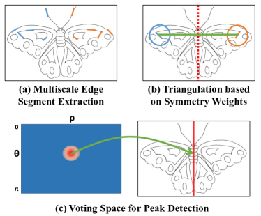
Figure 1: The general framework of the proposed reflection symmetry detection, using multi-scale edge detection followed by symmetry triangulation based on local geometrical, spatial and color information.

Log-Gabor filter was introduced by Field [11] in late 1980’s, as an alternative to the Gabor filter (formerly used in [10]), to suppress the effect of DC component through the computation of the multi-scale logarithmic function in the frequency domain. This process extracts more accurate feature (edge/corner) information from an image, plus ensuring the robustness of these features with respect to illumination variations. Feature extraction methods based on Log-Gabor filter have been successfully used in different computer vision applications (biometric authentication [13, 1], image retrieval [26], face recognition [15], image enhancement [27], character segmentation [18], and edge detection [12]).

Our contribution is twofold. Firstly, we extract edge features upon the application of Log-Gabor filters for symmetry detection instead of using Gabor filters. Secondly, we propose a similarity measure based on color image information, to improve the symmetry magnitude estimation in the voting step. In addition, we evaluate the proposed methods over all public datasets for reflection symmetry (single and multiple cases), in comparison with state-of-the-art algorithms.

Figure 1 shows our proposed algorithm, which detects globally the symmetry axes inside an image plane. We firstly extract edge features using Log-Gabor filters with different scales and orientations. Afterwards, we use the edge characteristics associated with the textural and color information as symmetrical weights for voting triangulation. In the end, we construct a polar-based voting histogram based on the accumulation of the symmetry contribution (local texture and color information), in order to find the maximum peaks presenting as candidates of the primary symmetry axes.

The remaining part of the paper is organized as follows. In section 2, we explain Log-Gabor transform and its feature-based application on a gray-scale image. In section 3, textural and color histograms of window-based features are described in details. In section 4, we illustrate the detection of symmetry candidates through triangulation and voting processes. Experimental details and results are presented in section 5. Finally, section 6 contains conclusion and future work.

2 Log-Gabor Edge Detection

Log-Gabor filter consists of logarithmic transformation of a Gabor filter in the Fourier domain, which suppresses the negative effect of the DC component:

$$\hat{G}(\eta,\alpha;s,o)=\hat{G}_{s}(\eta)\;\hat{G}_{o}(\alpha)$$ (1)

$$\hat{G}_{s}(\eta)=\exp(-\frac{(log(\frac{\eta}{\eta_{s}}))^{2}}{2(log(\sigma_{\eta}))^{2}})\>U(\eta)$$ (2)

$$\hat{G}_{o}(\alpha)=\exp(-\frac{|{atan(\frac{sin(\alpha-\alpha_{o})}{cos(\alpha-\alpha_{o})}})|}{2\sigma^{2}_{\alpha}})$$ (3)

where $(\eta,\alpha)$ are the log-polar coordinates representing radial and angular components over $S$ scales and $O$ orientations, associated with the frequency centers $(\eta_{s},\alpha_{o})$ and their bandwidths $(\sigma_{\eta},\sigma_{\alpha})$. $\hat{G}_{s}(\eta)$ is multiplied by low-pass Butterworth filter $U(\eta)$ of order $15$, and frequency $0.45$, to eliminate any extra frequencies at Fourier corners.

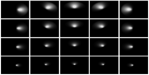
(a) Fourier

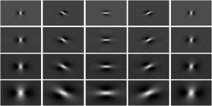
(b) Real

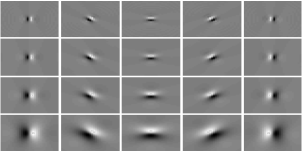
(c) Imaginary

Figure 2: Multi-resolution log-Gabor arrangement with $S=4$ scales (in rows) and $O=5$ orientations (in columns). (a) Filters in the Fourier domain. (b,c) Real and imaginary components in the spatial domain.

The modulus of complex wavelet coefficients $I_{s,o}(x,y)$ are computed on an image $I$ (width $W$ and height $H$) over multiple scales $s\in\{1,\ldots,S\}$ and orientations $o\in\{\frac{z\pi}{O},z=0,\ldots,O-1\}$ as follows:

$$I\;\;{\underset{GS}{\rightarrow}}\;\;I_{GS}\;\;{\overset{FT}{\rightarrow}}\;\;\hat{I}_{GS}$$ (4)

$$I_{s,o}(x,y)=|{FT}^{-1}(\hat{I}_{GS}\times\hat{G})|$$ (5)

where $\hat{I}_{GS}$ is the gray-scale version of the image $I$ in frequency domain, and ${FT}(.),\>{FT}^{-1}(.)\;$ are the Fourier transform and its inverse. Figure 2a shows Log-Gabor wavelet filter bank with $4$ scales and $5$ orientations where schematic contours cover the frequency space in the Fourier domain. Consequently, the elongation scheme of Log-Gabor wavelets appears in figures 2b, 2c presenting the real and imaginary components in the spatial domain.

(a) Input

(b) Amplitude

(c) Orientation

Figure 3: Log-Gabor response: (a) Input image. (b) Amplitude map $J\in[0,1]$. (c) Orientation map $\phi\in[-90^{\circ},90^{\circ}]$.

Figure 3 presents an example of Log-Gabor response $I_{s,o}$ on some natural image with a blurring background. Amplitude map $J(x,y)=\max\limits_{s,o}I_{s,o}(x,y)$ highlights the edge details of the foreground object in a sharp way, accompanied by precise angular values in the corresponding orientation map $\phi(x,y)$. Upon a spatial sampling of the input image $I$ using non-interleaved cells along a regular grid (stride and cell size are proportional to the maximum image dimension $\max(W,H)$). A feature point $p^{i}$ is extracted within each non-homogeneous cell $D_{i}$ using the wavelet response of Log-Gabor filter $I_{s,o}(D_{i})$, associated with its maximum wavelet response $J_{i}=J(p^{i})$ along side with the corresponding orientation $\phi_{i}$ and color in $HSV$ color space $\psi_{i}$.

3 Textural and Color Histograms

The textural and color information around an edge segment are prominent similarity characteristics for natural images, describing the symmetrical behavior of local edge orientation, and the balanced distribution of luminance and chrominance components. Hence, we introduce two histograms: Firstly, neighboring textural histogram $h^{i}$ of size $N$:

$$h^{i}(n)=\sum_{r\in D_{i}}J_{r}\;\mathbbm{1}_{\Phi_{n}}(\phi_{r}),$$ (6)

$$\Phi_{n}=[\frac{n\pi}{N},\frac{(n+1)\pi}{N}[,\;n=0,\ldots,N-1$$

where $\mathbbm{1}$ is the indicator function. $h^{i}$ is $l1$ normalized and circular shifted with respect to the orientation of the maximum magnitude $\phi_{i}$ among the neighborhood cell $D_{i}$. Secondly, the local $HSV$ histogram $g^{i}$ of size $C$ with sub-sampling rate ($C^{hu}:C^{sa}:C^{va}$)

$$g^{i}(c)=\sum_{r\in D^{*}_{i}}\mathbbm{1}_{\Psi_{c}}(\psi_{r}),$$ (7)

$$c =(c^{hu},c^{sa},c^{va}),$$

$$c^{hu} \in\{0,\ldots,C^{hu}-1\},$$

$$c^{sa} \in\{0,\ldots,C^{sa}-1\},$$

$$c^{va} \in\{0,\ldots,C^{va}-1\},$$

where $D^{*}_{i}$ is the neighborhood window around feature point $p^{i}$ , $\psi_{c}$ is a sub-sampled set of $HSV$ space, in terms of three components: hue ($hu$), saturation ($sa$) and value ($va$). $l1$ normalization is applied to $g^{i}(.)$ for bin-wise histogram comparison.

4 Symmetry Triangulation and Voting

A set of feature pairs $(p^{i},p^{j})$ of size $\frac{P(P-1)}{2}$ are elected such that $i\neq j$, and $P$ is the number of feature points. Then, we compute the symmetry candidate axis based a triangulation process with respect to the image origin. This candidate axis is parametrized by angle $\theta_{i,j}$ (orientation of the norm), and displacement $\rho_{i,j}$ (norm distance to the image origin) and has a symmetry weight $\omega_{i,j}$ defined as follows:

$$\omega_{i,j}=\omega(p^{i},p^{j})=m(i,j)\;t(i,j)\;q(i,j)$$ (8)

$$m(i,j) =|\tau^{i}R(T_{ij}^{\perp})\tau^{j}|$$ (9)

$$t(i,j) =\sum_{n=1}^{N}min(h^{i}(n),\tilde{h}^{j}(n))$$ (10)

$$q(i,j) =\sum_{c=1}^{C}min(g^{i}(c),g^{j}(c))$$ (11)

where $\tau^{i}$ is a direction vector associated with angle $\phi_{i}$, $R(T_{ij}^{\perp})$ is the reflection matrix with respect to the perpendicular of the line connecting $(p^{i},p^{j})$ [9, 10], and $\tilde{h}^{j}$ is the reverse version of $h^{j}$ histogram. $l1$ normalization is applied to symmetry weights $\omega$.

A symmetry histogram $H(\rho,\theta)$ is defined as the sum of the symmetry weights of all pairs of feature points such as:

$$H(\rho,\theta)=\sum_{\begin{subarray}{c}p^{i},p^{j}\\ i\neq{j}\end{subarray}}\omega_{i,j}\delta_{\rho-\rho_{i,j}}\delta_{\theta-\theta_{i,j}}$$ (12)

where $\delta$ is the Kronecker delta.

the voting histogram $H(\rho,\theta)$ is smoothed using a Gaussian kernel to output a proper density representation (as shown in figure 4), in which the major symmetry peaks are selected by reaching-out clear extreme spots using well-known non-maximal suppression technique [6]. The spatial boundaries of each symmetry axis is computed through the convex hull of the associated voting pairs.

(a) Input with GT

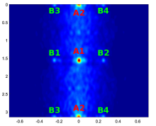
(b) Voting representation

Figure 4: Symmetry voting process: (a) Input image with major (in red) and minor (in green) symmetry axes. (b) Smoothed output of the symmetry histogram $H$ with $\rho$ displacement x-axis and $\theta$ angle y-axis, highlighting the corresponding axes.

5 Results and Discussions

This section describes the details of public symmetry datasets, evaluation metrics, and experimental settings for performance comparison of the proposed work. Performance analysis against the state-of-the-art algorithms is also provided in this section.

5.1 Datasets description

Seven public datasets of reflection symmetry detection are used from four different databases: (1) PSU datasets (single,multiple): Liu’s vision group proposed symmetry groundtruth for Flickr images (# images = # symmetries = 157 for single case, # images = 142 and # symmetries = 479 for multiple case) in ECCV2010, CVPR2011 and CVPR2013. (2) AVA dataset (single): Elawady et. al [10] provided axis groundtruth for some professional photographs (# images = # symmetries = 253 for single case) from large-scale aesthetic-based dataset called AVA [22]. (3) NY datasets (single,multiple): Cicconet et al. [8] introduced a symmetry database (# images = # symmetries = 176 for single case, # images = 63 and # symmetries = 188 for multiple case) in 2016, providing more stable groundtruth. (4) ICCV2017 training datasets (single,multiple): Seungkyu Lee delivered a challenge database associated with reflection groundtruth (# images = # symmetries = 100 for single case, # images = 100 and # symmetries = 384 for multiple case).

5.2 Evaluation metrics

Assuming a symmetry line defined by two endpoints $(a=[a_{x},x_{y}]^{T},\;b=[b_{x},b_{y}]^{T})$, quantitative comparisons are fundamentally performed by considering a detected symmetry candidate $SC=[a^{SC},b^{SC}]^{T}$ as a true positive (TP) respect to the corresponding groundtruth $GT=[a^{GT},b^{GT}]^{T}$ if satisfying the following two conditions:

$$T({atan}(\frac{{abs(\begin{vmatrix}v_{x}^{SC}&v_{x}^{GT}\\ v_{y}^{SC}&v_{y}^{GT}\end{vmatrix})}}{<v^{SC},v^{GT}>}))<\gamma\>,$$ (13)

$$\sqrt{(t_{x}^{SC}-t_{x}^{GT})^{2}+(t_{y}^{SC}-t_{y}^{GT})^{2}}<\zeta\>,$$ (14)

$$v^{SC}=(a^{SC}-b^{SC}),\>v^{GT}=(a^{GT}-b^{GT})\>,$$

$$t^{SC}=\frac{(a^{SC}+b^{SC})}{2},\>t^{GT}=\frac{(a^{GT}+b^{GT})}{2},$$

$$T(\Gamma)=\begin{cases}\pi-\Gamma,&\text{if }\Gamma>\frac{\pi}{2}\\ \Gamma,&\text{otherwise}\end{cases}$$

The conditions represent angular and distance constraints between detection and groundtruth axes. These constraints are upper-bounded by the corresponding thresholds $\gamma$ and $\zeta$, which are defined in table 1. Furthermore, the precision $PR$ and recall $RC$ rates are defined by selecting the symmetry peaks according to the candidates’ amplitude normalized by the highest detection score, to show the performance curve for each algorithm:

$$PR=\frac{TP}{TP+FP},\>RC=\frac{TP}{TP+FN}$$ (15)

where $FP$ is a false positive (non-matched detection), and $FN$ is a false negative (non-matched groundtruth). In addition, we used the maximum $F_{1}$ score identifying a unique comparison measure, to show the overall accuracy of each symmetry algorithm:

$${max}\{F_{1}\}={max}\{2\frac{PR\times RC}{PR+RC}\}$$ (16)

Table 1: Threshold values of evaluation metrics across different reflection symmetry competitions.

Competitions	$\gamma$	$\zeta$
CVPR2011 [25]	$10^{\circ}$	$20\%\times{len}(GT)$
CVPR2013 [16]	$10^{\circ}$	$20\%\times{min}\{{len}(MT),{len}(GT)\}$
ICCV2017	$3^{\circ}$	$2.5\%\times{min}\{W,H\}$

5.3 Experimental settings

We compare the proposed methods (Lg: without color information and LgC: with color information) against three state-of-the-art approaches: Loy and Eklundh (Loy2006) [17], Cicconet et al. (Cic2014) [9], and Elawady et al. (Ela2016) [10]). Their open-source codes are used with default parameter values for performance comparison. In Log-Gabor edge detection, we set the number of scales $S$ and number of orientations $O$ to $12$ and $32$. We also set the radial bandwidth $\sigma_{\eta}$ to $0.55$ and the angular bandwidth $\sigma_{\alpha}$ to $0.2$. In textural and color histogram calculations, we define the number of bins for textural $N$ and color $C$ to $32$ and $32$ (sampling rate $C^{hu}:C^{sa}:C^{va}=8:2:2$) respectively. In case of gray-scale images, contrast values are used instead of color information in $HSV$ color space. In symmetry voting, we declare the 2D histogram space of $\rho=\sqrt{W^{2}+H^{2}}$ displacement bins and $\theta=360$ orientation bins for extrema selection.

5.4 Performance analysis

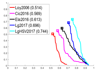
(a) PSU

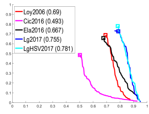
(b) AVA

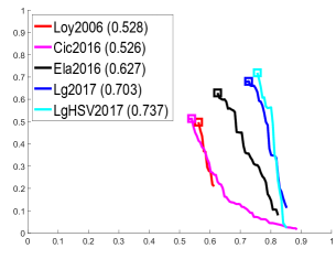
(c) NY

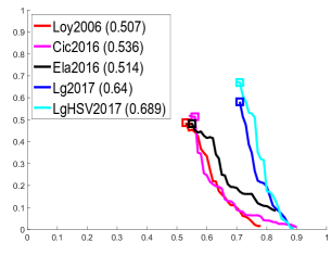
(d) ICCV’17

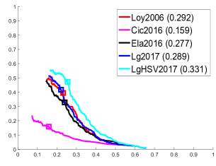
(e) PSUm

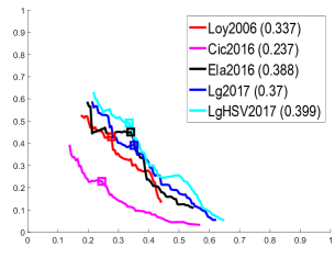
(f) NYm

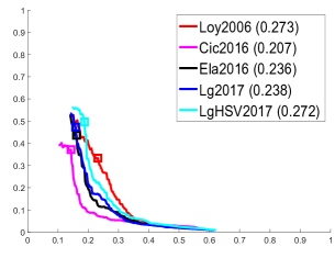
(g) ICCV’17m

Figure 5: Using evaluation metrics CVPR2013 [16], Precision-Recall curves on: (1) four single-case symmetry (a,b,c,d) datasets, and (2) three multiple-case symmetry (e,f,g) datasets to show the overall superior performance of our proposed methods ( Lg2017 and LgHSV2017) against the three prior algorithms (Loy2006 [17], Cic2014 [9], and Ela2016 [10]). The maximum F1 scores are qualitatively presented as square symbols along the curves, and quantitatively indicated between parentheses inside the top-right legends. Best seen on screen (zoom-in for details).

Table 2: Using evaluation metrics CVPR2013 [16], comparison of the true positive rates based on top detection for the proposed methods against the state-of-art algorithms. Symmetry datasets are presented as: single-case (first 4 rows) and multiple-case (last 3 rows), highlighted between (parenthesis) the number of images for each dataset. Top 1st and 2nd values are in Bold and underlined respectively.

Datasets	Loy[17]	Cic[9]	Ela[10]	Lg	LgC
PSU(157)	81	90	97	109	116
AVA(253)	174	124	170	191	197
NY(176)	98	92	109	125	132
ICCV17(100)	52	53	52	70	69
PSUm(142)	69	68	67	74	79
NYm(63)	32	36	36	39	40
ICCV17m(100)	54	39	53	53	56

Table 3: Using evaluation metrics ICCV17, comparison of the true positive rates based on top detection in single-case and all detections in multiple-case for the proposed methods against the state-of-art algorithms. Symmetry datasets are presented as: single-case (first 4 rows) and multiple-case (last 3 rows), highlighted between (parenthesis) the number of groundtruth for each dataset. Top 1st and 2nd values are in Bold and underlined respectively.

Datasets	Loy[17]	Cic[9]	Ela[10]	Lg	LgC
PSU(157)	41	27	46	52	51
AVA(253)	63	36	95	86	87
NY(176)	34	35	43	50	53
ICCV17(100)	17	9	19	22	22
PSUm(479)	130	65	129	154	157
NYm(188)	48	45	69	57	60
ICCV17m(384)	95	38	86	111	111

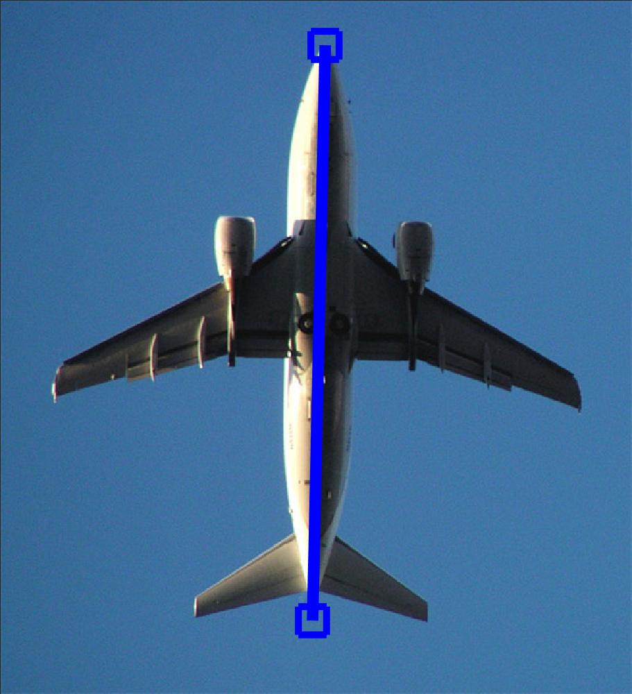
(a) 16550 - GT

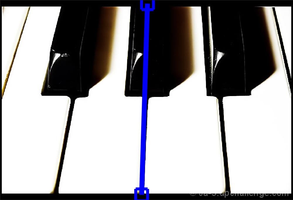
(b) 832486 - GT

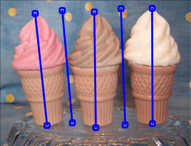
(c) ref_rm_13 - GT

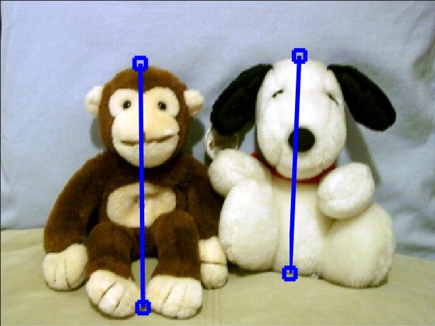
(d) ref_rm_65 - GT

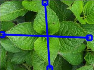
(e) I034 - GT

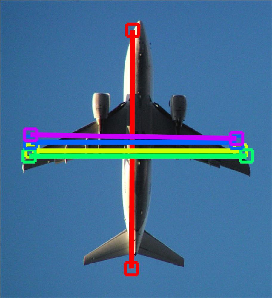
(f) 16550 - LgC

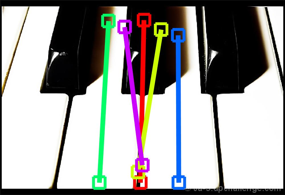
(g) 832486 - LgC

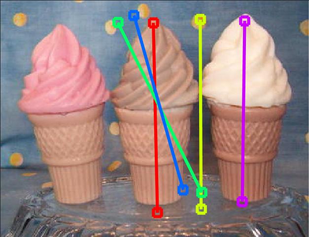
(h) ref_rm_13 - LgC

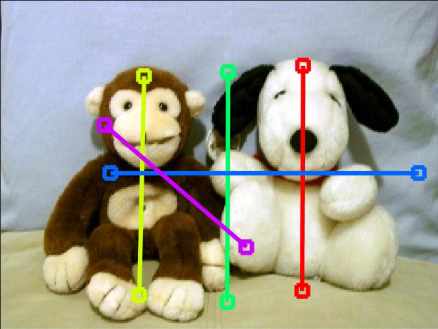
(i) ref_rm_65 - LgC

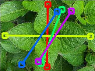
(j) I034 - LgC

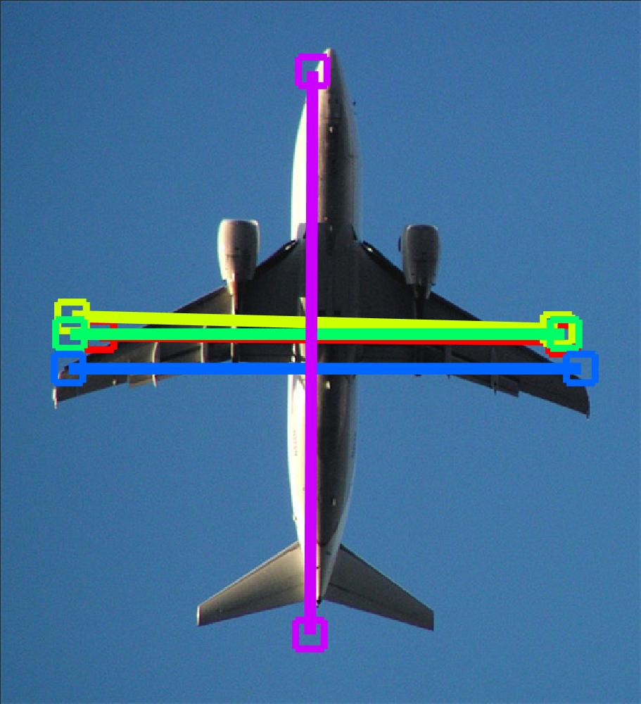
(k) 16550 - Lg

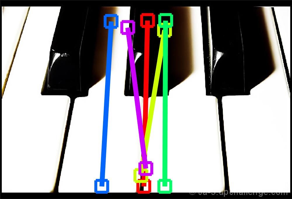
(l) 832486 - Lg

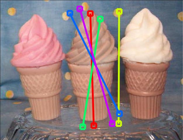
(m) ref_rm_13 - Lg

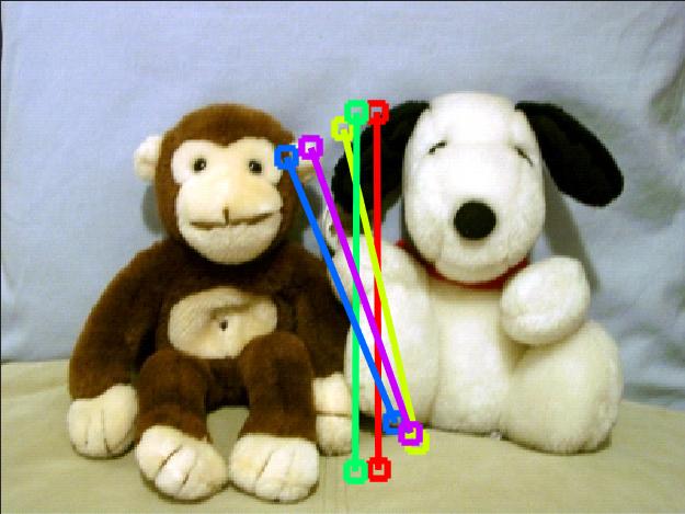
(n) ref_rm_65 - Lg

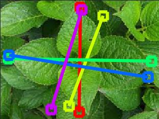
(o) I034 - Lg

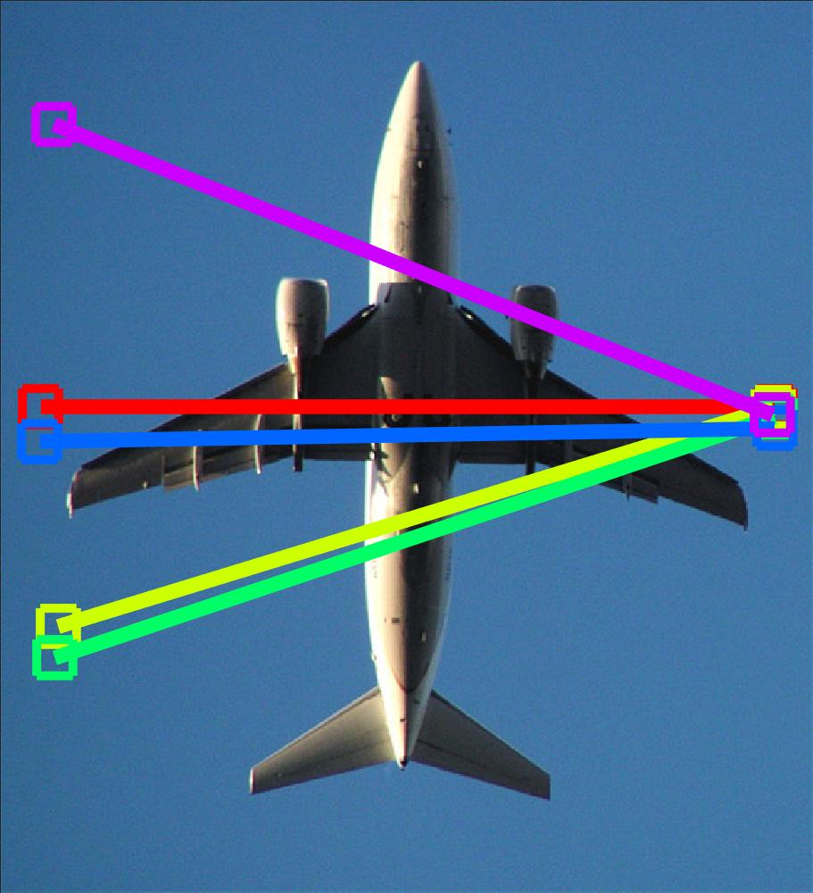
(p) 16550 - Ela

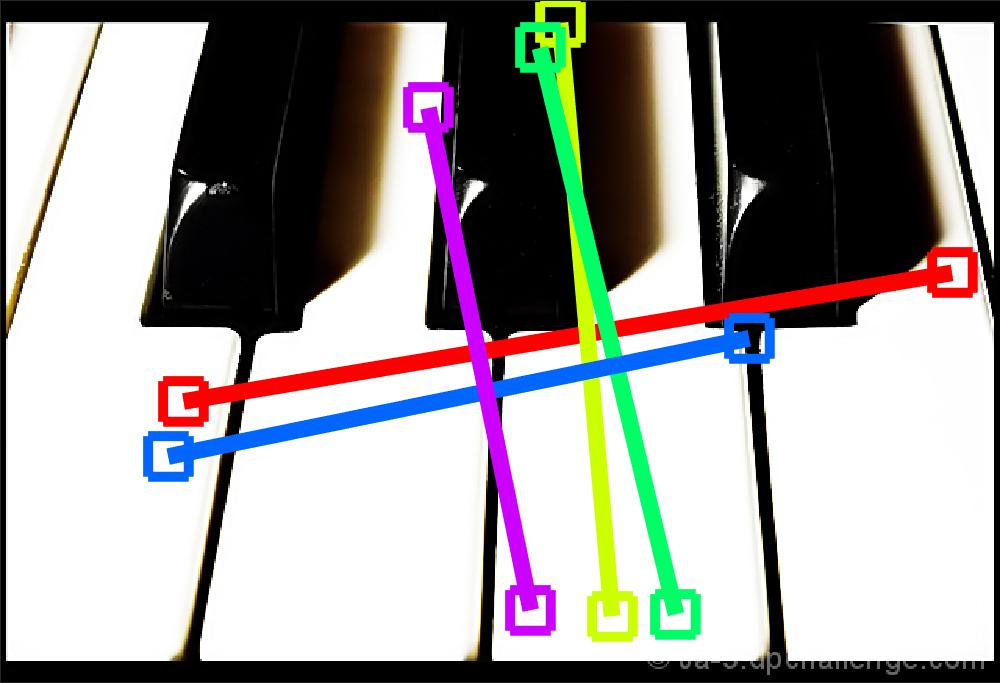
(q) 832486 - Ela

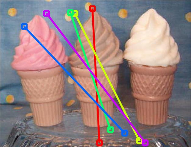
(r) ref_rm_13 - Ela

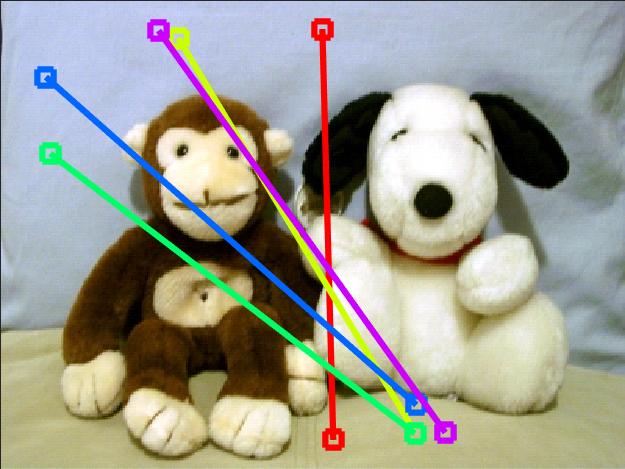
(s) ref_rm_65 - Ela

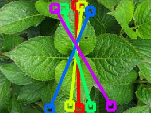
(t) I034 - Ela

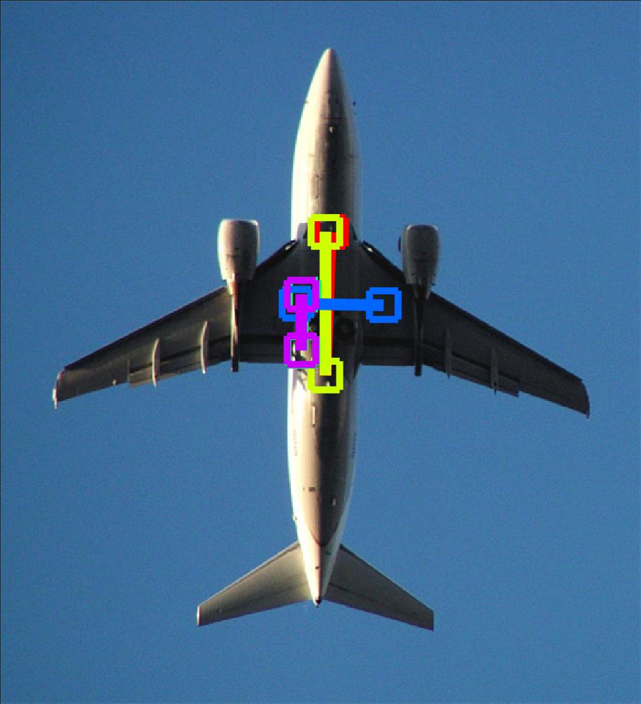
(u) 16550 - Loy

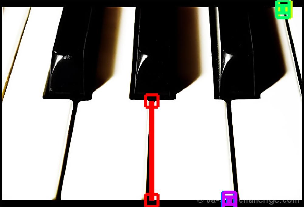
(v) 832486 - Loy

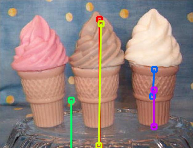
(w) ref_rm_13 - Loy

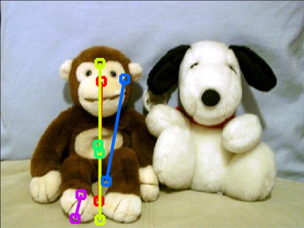
(x) ref_rm_65 - Loy

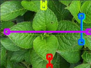
(y) I034 - Loy

Figure 6: Some single-case and multiple-case results from AVA [10], PSUm [25, 16], and NYm [8] datasets with groundtruth ( blue) in 1st row (a-e). our methods in 2nd and 3rd rows (f-o) produces better results among El2016 [10] in 4rd row (p-t) and Loy2006 [17] in 5th row (u-y). For each algorithm, the top five symmetry results is presented in such order: red, yellow, green, blue, and magenta. Each symmetry axis is shown in a straight line with squared endpoints. Best seen on screen.

In our experimental evaluation, the algorithms are executed to detect and compare the global symmetries inside synthetic and real-world images. Tables 2, 3 show the different versions of true positive rates for the proposed methods (Lg and LgC) against Loy and Eklundh (Loy) [17], Cicconet et al. (Cic) [9], and Elawady et al. (Ela) [10]. LgC performs the best result among most cases in single and multiple symmetry, due to the importance of color information for the voting computations in colorful images. At the same time, Lg has the top 2nd result, and sometimes the top 1st results in gray-scale or low-saturated images. Ela [10] ranked as the top 3rd result, due to the utilization of small grids to compute window-based features. Thanks for the advantage of SIFT features, Loy [17] is still strong competent to be ranked as the top 4th result in general. Cic [9] has the lowest performance.

Figure 5 presents performance results in terms of precision and recall curves for single-case and multiple-case symmetry datasets, plus values of the maximum $F_{1}$ score to measure the performance of the proposed algorithms (Lg2017 and LgHSV2017) against Loy and Eklundh (Loy2006) [17], Cicconet et al. (Cic2014) [9], and Elawady et al. (Ela2016) [10]. In single-case symmetry, our method Lg2017 outperforms the other concurrent algorithms (Loy2006, Cic2014, and Ela2016) in the context of using only gray-scale version of involved images. Furthermore, color version of our method LgHSV2017 exploits slightly improvement over gray-scale one Lg2017. On the other hand, Only LgHSV2017 has better precision performance among others in (PSUm and NYm) datasets, due to many local symmetry groundtruth presenting inside multiple-case symmetry.

As a summary of the previous quantitative evaluations, figure 6 compares qualitatively top performing algorithms showing different examples of reflection symmetry detection. Despite the single-case images (1st and 2nd columns) have strong shadowing effect in foreground objects, the color version of the proposed method LgC easily finds the correct symmetry axes as a first candidate. On the other hand, the non-color proposed method Lg satisfies the single-symmetry groundtruth in the two examples as first and fifth detections respectively. In contrast, Ela [10] mismatches the provided groundtruth with all detection and Loy [17] only finds the local symmetry axes in the object parts having same contrast values. In multiple-case images (3rd, 4th and 5th columns), LgC clearly detects the global and most of local symmetries. In the opposite side, the other methods struggle determining only more than one correct groundtruth.

6 Conclusion

In this paper, we detect global symmetry axes inside an image using the edge characteristics of Log-Gabor wavelet response. For the purpose of improving our results, we additionally use textural and color histograms as local symmetrical measure around edge features. We show that the proposed methods provide a great improvement over single and multiple symmetry cases in all public datasets. Future work will focus on improving the voting representations, respect to the number of symmetry candidate pairs, resulting a precise selection of symmetrical axis peaks and their corresponding voting features. For art and aesthetic ranking applications, a unified balance measure is required to describe the global symmetry degree inside an image.

References

- [1] N. U. Ahmed, S. Cvetkovic, E. H. Siddiqi, A. Nikiforov, and I. Nikiforov. Combining iris and periocular biometric for matching visible spectrum eye images. Pattern Recognition Letters, 91:11–16, 2017.
- [2] R. Arnheim. Art and visual perception. Stockholms Universitet, Institutionen för Konstvetenskap, 2001.
- [3] I. Atadjanov and S. Lee. Bilateral symmetry detection based on scale invariant structure feature. In Image Processing (ICIP), 2015 IEEE International Conference on, pages 3447–3451. IEEE, 2015.
- [4] I. R. Atadjanov and S. Lee. Reflection symmetry detection via appearance of structure descriptor. In European Conference on Computer Vision, pages 3–18. Springer, 2016.
- [5] D. Cai, P. Li, F. Su, and Z. Zhao. An adaptive symmetry detection algorithm based on local features. In Visual Communications and Image Processing Conference, 2014 IEEE, pages 478–481. IEEE, 2014.
- [6] J. Canny. A computational approach to edge detection. IEEE Transactions on pattern analysis and machine intelligence, (6):679–698, 1986.
- [7] M. Cho and K. M. Lee. Bilateral symmetry detection via symmetry-growing. In BMVC, pages 1–11. Citeseer, 2009.
- [8] M. Cicconet, V. Birodkar, M. Lund, M. Werman, and D. Geiger. A convolutional approach to reflection symmetry. Pattern Recognition Letters, 2017.
- [9] M. Cicconet, D. Geiger, K. C. Gunsalus, and M. Werman. Mirror symmetry histograms for capturing geometric properties in images. In Computer Vision and Pattern Recognition (CVPR), 2014 IEEE Conference on, pages 2981–2986. IEEE, 2014.
- [10] M. Elawady, C. Barat, C. Ducottet, and P. Colantoni. Global bilateral symmetry detection using multiscale mirror histograms. In International Conference on Advanced Concepts for Intelligent Vision Systems, pages 14–24. Springer, 2016.
- [11] D. J. Field. Relations between the statistics of natural images and the response properties of cortical cells. Josa a, 4(12):2379–2394, 1987.
- [12] X. Gao, F. Sattar, and R. Venkateswarlu. Multiscale corner detection of gray level images based on log-gabor wavelet transform. IEEE Transactions on Circuits and Systems for Video Technology, 17(7):868–875, 2007.
- [13] H. Kaur and P. Khanna. Cancelable features using log-gabor filters for biometric authentication. Multimedia Tools and Applications, 76(4):4673–4694, 2017.
- [14] S. Kondra, A. Petrosino, and S. Iodice. Multi-scale kernel operators for reflection and rotation symmetry: further achievements. In Computer Vision and Pattern Recognition Workshops (CVPRW), 2013 IEEE Conference on, pages 217–222. IEEE, 2013.
- [15] J. Li, N. Sang, and C. Gao. Log-gabor weber descriptor for face recognition. Journal of Electronic Imaging, 24(5):053014–053014, 2015.
- [16] J. Liu, G. Slota, G. Zheng, Z. Wu, M. Park, S. Lee, I. Rauschert, and Y. Liu. Symmetry detection from realworld images competition 2013: Summary and results. In Computer Vision and Pattern Recognition Workshops (CVPRW), 2013 IEEE Conference on, pages 200–205. IEEE, 2013.
- [17] G. Loy and J.-O. Eklundh. Detecting symmetry and symmetric constellations of features. In Computer Vision–ECCV 2006, pages 508–521. Springer, 2006.
- [18] C. Mancas-Thillou and B. Gosselin. Character segmentation-by-recognition using log-gabor filters. In Pattern Recognition, 2006. ICPR 2006. 18th International Conference on, volume 2, pages 901–904. IEEE, 2006.
- [19] E. Michaelsen, D. Muench, and M. Arens. Recognition of symmetry structure by use of gestalt algebra. In Computer Vision and Pattern Recognition Workshops (CVPRW), 2013 IEEE Conference on, pages 206–210. IEEE, 2013.
- [20] Y. Ming, H. Li, and X. He. Symmetry detection via contour grouping. In Image Processing (ICIP), 2013 20th IEEE International Conference on, pages 4259–4263. IEEE, 2013.
- [21] Q. Mo and B. Draper. Detecting bilateral symmetry with feature mirroring. In CVPR 2011 Workshop on Symmetry Detection from Real World Images, 2011.
- [22] N. Murray, L. Marchesotti, and F. Perronnin. Ava: A large-scale database for aesthetic visual analysis. In Computer Vision and Pattern Recognition (CVPR), 2012 IEEE Conference on, pages 2408–2415. IEEE, 2012.
- [23] M. Park, S. Lee, P.-C. Chen, S. Kashyap, A. A. Butt, and Y. Liu. Performance evaluation of state-of-the-art discrete symmetry detection algorithms. In Computer Vision and Pattern Recognition, 2008. CVPR 2008. IEEE Conference on, pages 1–8. IEEE, 2008.
- [24] V. Patraucean, R. G. von Gioi, and M. Ovsjanikov. Detection of mirror-symmetric image patches. In Computer Vision and Pattern Recognition Workshops (CVPRW), 2013 IEEE Conference on, pages 211–216. IEEE, 2013.
- [25] I. Rauschert, K. Brocklehurst, S. Kashyap, J. Liu, and Y. Liu. First symmetry detection competition: Summary and results. Technical report, Technical Report CSE11-012, Department of Computer Science and Engineering, The Pennsylvania State University, 2011.
- [26] E. Walia and V. Verma. Boosting local texture descriptors with log-gabor filters response for improved image retrieval. International Journal of Multimedia Information Retrieval, 5(3):173–184, 2016.
- [27] W. Wang, J. Li, F. Huang, and H. Feng. Design and implementation of log-gabor filter in fingerprint image enhancement. Pattern Recognition Letters, 29(3):301–308, 2008.
- [28] Z. Wang, Z. Tang, and X. Zhang. Reflection symmetry detection using locally affine invariant edge correspondence. Image Processing, IEEE Transactions on, 24(4):1297–1301, 2015.
- [29] R. D. Zakia and D. Page. Photographic Composition: A Visual Guide. Taylor & Francis, 2010.