Asymptotic Floquet states of non-Markovian systems

Abstract

We propose a method to find asymptotic states of a class of periodically modulated open systems which are outside the range of validity of the Floquet theory due to the presence of memory effects. The method is based on a Floquet treatment of the time-local, memoryless dynamics taking place in a minimally enlarged state space where the original system is coupled to auxiliary – typically non-physical – variables. A projection of the Floquet solution into the physical subspace returns the sought asymptotic state of the system. The spectral gap of the Floquet propagator acting in the enlarged state space can be used to estimate the relaxation time. We illustrate the method with a modulated version of quantum random walk model.

I Introduction

Periodically driven systems can exhibit a spectrum of states which are unattainable in the static limit. This makes the idea of modulations appealing to various fields, ranging from dynamical chaos theory Kadanoff1993 and chemical kinetics Petrov et al. (1997) to neuroscience Herrmann (2001) and quantum physics  Shirley (1965); Sambe (1973); Grifoni and Hänggi (1998); Bukov et al. (2015); Eckardt and Anisimovas (2015). In the latter field, periodic driving was used to realize new topological states Lindner et al. (2011); Liu et al. (2013), engineer artificial gauge fields Struck et al. (2011); Goldman and Dalibard (2014), and create so-called ‘Floquet time crystals’ Else et al. (2016); Zhang et al. (2017); Choi et al. (2017).
Typically, one models periodically modulated systems via linear differential equations with time-periodic coefficients whose solution is provided by Floquet theory Floquet (1883); Yakubovich and Starzhinskii (1975). The key prerequisite to construct such a model is the time-local character of the system dynamics which means that the future of the system depends on its current state and not on its history. For a system with time-local and contractive (in terms of some proper norm) dynamics, the fate of the system is specified by the asymptotic state(s). A periodically modulated system interacting with a broadband environment in the Markovian limit, evolves towards an asymptotic state which is periodic with the period of the modulations Jung (1993); Gammaitoni et al. (1998); Hartmann et al. (2017). On the model level, this state represents a limit cycle solution of the dissipative equations describing the system dynamics Yakubovich and Starzhinskii (1975). Very recently, an idea to combine modulations and dissipation to explore many-body quantum states Vorberg et al. (2013); Lazarides and Moessner (2017) has emerged as a natural extension of the established Hamiltonian-oriented approach Goldman and Dalibard (2014); Bukov et al. (2015); Sommer and Simon (2016); Meinert et al. (2016); Eckardt (2017). Still, the use of Floquet theory in the dissipative context implies that the equations used to describe the dynamics remain local in time Kohler et al. (2005); Alicki and Lendi (2007); Bastidas et al. (2017).
What are the asymptotic Floquet states of systems governed by time-nonlocal evolution equations? This question is of a special relevance in the context of quantum non-Markovian dynamics, a topic being actively explored now both in theoretical Breuer et al. (2016) and experimental Liu2011 domains. Here we present a method to get the answer for a broad class of periodically modulated systems whose evolution is governed by memory-kernel master equations. We show that the corresponding asymptotic solutions possess the periodicity of the modulations and have the form prescribed by the recently introduced generalized Floquet theorem (gFT) Traversa et al. (2013).

II Method

We consider physical systems, both classical and quantum, whose state is described by a $n$-dimensional vector $\mathbf{x}(t)$ obeying a generalized master equation of the form

$$\dot{\mathbf{x}}(t)=\int_{t_{0}}^{t}dt^{\prime}\mathbf{K}(t,t^{\prime})\mathbf{x}(t^{\prime})+\mathbf{z}(t)\;,$$ (1)

with an integrable memory kernel (MK) matrix $\mathbf{K}(t,t^{\prime})$ and an asymptotically vanishing inhomogeneous term, $\lim_{t\rightarrow\infty}\mathbf{z}(t)=\mathbf{0}$ . The vector $\mathbf{x}(t)$ may describe, for example, a $n$-state classical system or the density matrix of a quantum system in a suitable representation Vacchini (2013, 2016). We assume the MK to be biperiodic, i.e., $\mathbf{K}(t+T,t^{\prime}+T)=\mathbf{K}(t,t^{\prime})$, where $T$ denotes the period of the modulation. The above requirements ensure that, in the limit $t\rightarrow\infty$, the action of the operator $\mathcal{L}_{t}\{\mathbf{x}(t)\}=\int_{t_{0}}^{t}dt^{\prime}\mathbf{K}(t,t^{\prime})\mathbf{x}(t^{\prime})+\mathbf{z}(t)$ commutes with that of the one-period translation operator $\mathcal{S}_{T}\{\mathbf{x}(t)\}=\mathbf{x}(t+T)$, thus entailing the applicability of the gFT to the asymptotic dynamics induced by Eq. (1) note1 . Note that the condition of biperiodicity is automatically satisfied if the MK depends exclusively on the difference $\tau=t-t^{\prime}$ or if the MK is periodic with respect to $t$ ($t^{\prime}$) and depends only on $t$ ($t^{\prime}$) and $\tau$.
Our approach to determine the asymptotic solution of Eq. (1) is based on the idea of embedding the system into an enlarged state space where the physical variable $\mathbf{x}(t)$ is coupled to an auxiliary vector variable $\mathbf{u}(t)$. The coupling is realized in such a way that the resulting extended system described by the new vector $\mathbf{v}^{\rm T}(t)=[\mathbf{x}^{\rm T}(t),\mathbf{u}^{\rm T}(t)]$ (concatenation) obeys a time-local equation satisfying the conditions of the standard Floquet theorem. The latter provides the solution for the state of the extended vector $\mathbf{v}(t)$ whose projection into the physical $\mathbf{x}$-subspace constitutes the asymptotic Floquet state of the system.

The concept of embedding is well known within the theory of classical stochastic processes Grabert et al. (1977, 1978, 1980); Grigolini (1982); Kupferman (2004); Siegle et al. (2010) where it is related to celebrated Erlang’s method of stages Cox and Miller (1977). Embedding schemes are also employed Breuer (2004); Budini (2013); Kretschmer et al. (2016) in the recently established field of quantum non-Markovian processes Breuer2008 ; Vacchini (2016); Breuer et al. (2016). However, in the above cases the embedding is physical, i.e., the new auxiliary variables (states or degrees of freedom) have the same physical meaning as the original variable(s). In other words, the enlarged system is obtained by attaching ancillas to the original system, see, e.g., Ref. Budini (2013). In the quantum case, such physical embedding might be very hard (or not possible) to construct for a given kernel and, even when constructed, it might be very complicated to deal with. Here we do not restrict ourselves to the physical embedding. Instead we propose a minimal enlargement of the system, by introducing a set of non-physical auxiliary variables, which leads to a new set of equations, now local in time.
For the $n\times n$ MK matrix in Eq. (1) we consider the following structure

$$\mathbf{K}(t,t^{\prime})=\sum_{j=1}^{k}\Gamma_{j}e^{-\gamma_{j}(t-t^{\prime})}\mathbf{E}_{j}(t)\mathbf{F}_{j}(t^{\prime})\;,$$ (2)

with $\Gamma_{j},\gamma_{j}\in\mathbb{C}$ and $\mathbf{E}_{j}(t)=\mathbf{E}_{j}(t+T)$, $\mathbf{F}_{j}(t)=\mathbf{F}_{j}(t+T)\in\mathbb{C}^{n\times n}$. In the stationary case, $\mathbf{E}_{j}(t)\equiv\mathbf{E}_{j}$ and $\mathbf{F}_{j}(t^{\prime})\equiv\mathbf{F}_{j}$, this form relates to Erlang’s method of stages Cox (1955). The structure given by Eq. (2) allows to reproduce – exactly or arbitrary well – a large class of memory kernels, including oscillatory ones Beylkin and Monzón (2005).
With the kernel (2), the time evolution given by Eq. (1) for the physical system described by $\mathbf{x}$ is equivalently obtained by solving a time-local set of equations in which the $n$-dimensional vector $\mathbf{x}$ is coupled to an auxiliary variable $\mathbf{u}$ of the dimension $p=n\times k$. The equations for the extended system read (from now on we set $t_{0}=0$)

$$\left\{\begin{array}[]{lr}\dot{\mathbf{x}}(t)=-\mathbf{H}(t)\mathbf{u}(t)\\ \dot{\mathbf{u}}(t)=-\mathbf{G}(t)\mathbf{x}(t)-\mathbf{A}\mathbf{u}(t)\;,\end{array}\right.$$ (3)

where $\mathbf{H}(t)=(\Gamma_{1}\mathbf{E}_{1}(t),\dots,\Gamma_{k}\mathbf{E}_{k}(t))$, $\mathbf{G}^{\rm T}(t)=(\mathbf{F}^{\rm T}_{1}(t),\dots,\mathbf{F}^{\rm T}_{k}(t))$, and $\mathbf{A}=\rm diag(\gamma_{1}\mathbf{1}^{n\times n},\dots,\gamma_{k}\mathbf{1}^{n\times n})$.
To assess the equivalence of Eqs. (1) and (3) we set $\mathbf{G}(t)\mathbf{x}(t)\equiv\mathbf{w}(t)$ and note that the equation for $\mathbf{u}$ reads in Laplace space $\mathbf{u}(\lambda)=\left[\lambda\mathbf{1}+\mathbf{A}\right]^{-1}\mathbf{u}(0)-\left[\lambda\mathbf{1}+\mathbf{A}\right]^{-1}\mathbf{w}(\lambda)$. Going back to the time domain, multiplying the resulting equation to the left by $-\mathbf{H}(t)$, and using the first of equations (3), we end up with Eq. (1) with $\mathbf{K}(t,t^{\prime})=\mathbf{H}(t)e^{-\mathbf{A}(t-t^{\prime})}\mathbf{G}(t^{\prime})$, provided that the following relation is satisfied

$$\mathbf{z}(t)=-\mathbf{H}(t)e^{-\mathbf{A}t}\mathbf{u}(0)\;.$$ (4)

Thus, the requirement for the evolution of the physical part $\mathbf{x}(t)$ of the enlarged system to coincide with that given by Eq. (1), fixes the initial condition for the auxiliary variable $\mathbf{u}(t)$.
The system of equations (3) can be put into the compact form

$$\dot{\mathbf{v}}(t)=\mathbf{M}(t)\mathbf{v}(t)\;,$$ (5)

where $\mathbf{v}=(x_{1},\dots,x_{n},u_{1},\dots,u_{nk})^{\rm T}$ is the $(p=n+nk)$-dimensional vector describing the enlarged system, with the matrix $\mathbf{M}$ assuming the block structure

$$\mathbf{M}(t)=\left(\begin{array}[]{lr}\quad\mathbf{0}\quad-\mathbf{H}(t)\\ -\mathbf{G}(t)\quad\mathbf{A}\end{array}\right)$$ (8)

where $\mathbf{0}\in\mathbb{R}^{n\times n}$. A memory kernel of the form (2), with $T$-periodic $\mathbf{E}(t)$ and $\mathbf{F}(t)$, entails the $T$-periodicity for the matrix $\mathbf{M}(t)$. This in turn ensures that Eq. (5) qualifies to invoke the Floquet theorem which leads to a solution of the form $\mathbf{v}(t)=\tilde{\mathbf{S}}(t,0)e^{\mathbf{R}t}\mathbf{v}(0)$, where $\tilde{\mathbf{S}}(t,0)$ is a $T$-periodic $p\times p$ matrix and $\mathbf{R}$ a constant $p\times p$ matrix Yakubovich and Starzhinskii (1975). The projection of the vector $\mathbf{v}(t)$ onto the physical manifold, $\mathcal{P}_{\mathbf{x}}\mathbf{v}(t)=\mathbf{x}(t)$, yields for the solution in the original state space,

$$\mathbf{x}(t)=\mathbf{S}(t,0)e^{\mathbf{R}t}\mathbf{v}(0)\;,$$ (9)

with a $n\times p$ matrix $\mathbf{S}=\mathcal{P}_{\mathbf{x}}\tilde{\mathbf{S}}$. This is the form expected from the gFT Traversa et al. (2013). In the time-local limit, i.e., $\mathbf{K}(t,t^{\prime})=\delta(t-t^{\prime})\mathbf{K}_{\rm t.l.}(t)$, the solution reduces to the standard Floquet form, with $p=n$ Yakubovich and Starzhinskii (1975).
Equation (5) can be solved by constructing the Floquet propagator $\mathbf{U}_{T}=\mathcal{T}\exp[\int_{0}^{T}\mathbf{M}(\tau)d\tau]$, where $\cal{T}$ denotes the time-ordering operator, and then finding its invariant, $\mathbf{U}_{T}\mathbf{y}=\mathbf{y}$ Yakubovich and Starzhinskii (1975). This vector yields the asymptotic solution at stroboscopic instants of time, i.e., $\mathbf{y}=\mathbf{v}^{\mathrm{a}}(sT)$, $s\in\mathbb{Z}$. The spectral properties of the propagator can be used to characterize the relaxation time towards the asymptotic state. A conventional candidate is the spectral gap Levin et al. (2008), $g=1-|\lambda_{m}|$, with $\lambda_{m}$ being the second largest (by absolute value) eigenvalue of $\mathbf{U}_{T}$ after $\lambda_{1}=1$. A straightforward diagonalization of the propagator and the use of the obtained $\lambda_{m}$ as the quantifier of the relaxation speed is not suitable in our case. This is because this eigenvalue addresses the whole enlarged space, including the part which is not accessible with any physically meaningful initial condition. To address the physical manifold only, we suggest the Arnoldi iteration method, starting with the initial vector $\mathbf{v}^{\rm T}(0)=[\mathbf{x}^{\rm T}(0),\mathbf{u}^{\rm T}(0)]$, where $\mathbf{u}(0)$ satisfies Eq. (4), with consecutive diagonalization of the Hessenberg matrix Golub and Van Loan (1996).

III Application: Periodically driven quantum random walk

Here we apply the method described above to the non-Markovian master equation for a continuous time quantum random walk model which yields, by construction, a completely positive and trace preserving (CPT) quantum evolution Budini (2004); Vacchini (2013). The model has a direct interpretation in terms of an operator generalization of a classical semi-Markov process, a multi-site jump process defined by a transition matrix and a waiting time distribution (WTD) $f$ Vacchini (2012, 2016). This classical process is itself described by a generalized master equation of the form (1) and turns out to be Markovian only for exponentially distributed waiting times $\tau$ between consecutive jumps, i.e., $f(\tau)=\lambda\exp(-\lambda\tau)$.
In our application, a qubit whose density matrix $\rho(t)$ undergoes a trivial continuous background evolution (provided by the identity map $\mathbb{1}$), interrupted by the instantaneous actions of a CPT map $\mathcal{E}$  Budini (2004); Vacchini (2013). These ’collisions’ occur at random instances of time, with the time intervals between consecutive collisions distributed according to a WTD of the bi-exponential form

$$f(\tau)=\frac{2A}{a}e^{-\gamma\tau/2}\sinh(a\tau/2)\;,$$ (10)

with $a=\sqrt{\gamma^{2}-4A}>0$.

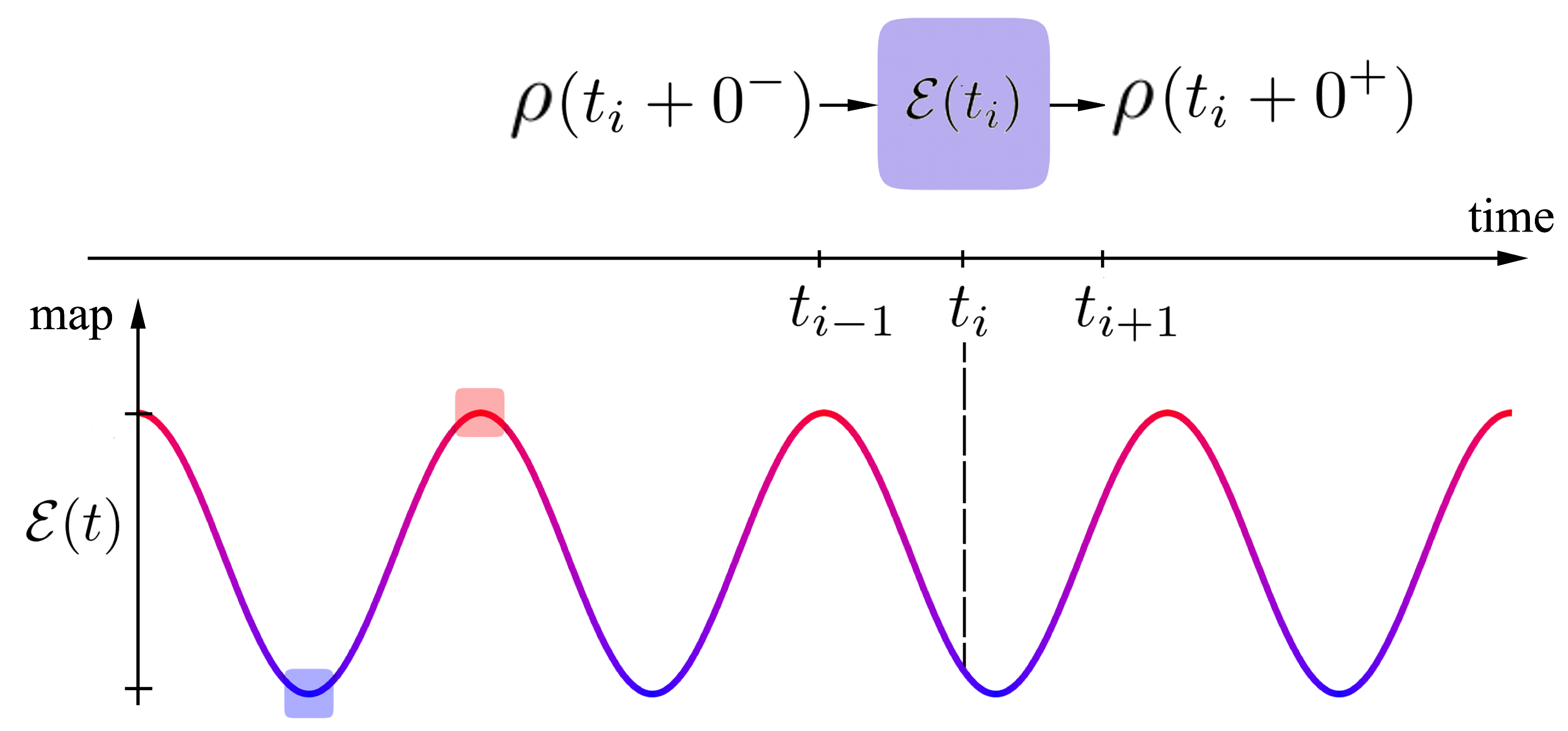
Figure 1: (color online) Continuous time quantum random walk with a time-periodic map. A qubit undergoes repeated instantaneous actions of a time-dependent map $\mathcal{E}(t)$ at random instances of times $...t_{i-1},t_{i},t_{i+1},...$. The time interval between consecutive collisions, $\tau_{i}=t_{i+1}-t_{i}$, is controlled by a waiting time distribution $f(\tau)$. There is no evolution of the qubit in between collisions. The map $\mathcal{E}(t)$ is obtained as a convex combination of constant CPT maps (in this case, of two maps labelled by colored squares), with time-periodic coefficients. Averaging over an infinite number of realizations of the process results in the master equation (14).

We generalize the original model Budini (2004); Vacchini (2013) by assuming that the collision map itself periodically evolves in time, $\mathcal{E}(t+T)=\mathcal{E}(t)$; see Fig. 1. The time-periodic CPT $\mathcal{E}(t)$ can be constructed as a convex combination of $L$ CPT maps $\mathcal{E}(t)=\sum_{s}^{L}l_{s}(t)\mathcal{E}_{s}$, where $l_{s}(t)\geq 0$, $\sum_{s}^{L}l_{s}(t)=1$ for $\forall t\in[0,T]$, and $l_{s}(t+T)=l_{s}(t)$. Note that, in order to get a nontrivial asymptotic state, $\rho^{\mathrm{a}}(t)\neq\mathbb{1}/2$, at least one of the maps $\mathcal{E}_{s}$ has to be non-unital. We choose the following time-periodic map

$$\mathcal{E}(t)=l_{1}(t)\mathcal{E}_{1}+l_{2}(t)\mathcal{E}_{2}+l_{3}(t)\mathcal{E}_{3}\;,$$ (11)

with $l_{1}(t)=\sin^{2}(\Omega t)$, $l_{2}=\sin^{2}(\Omega t)\cos^{2}(\Omega t)$, and $l_{3}=\cos^{4}(\Omega t)$, so that $T=\pi/\Omega$. The map $\mathcal{E}_{1}$ is the non-unital amplitude damping map defined by the following action on the $2\times 2$ qubit density matrix Nielsen and Chuang (2010)

$$\mathcal{E}_{1}[\rho] = M_{0}\rho M_{0}^{{\dagger}}+M_{1}\rho M_{1}^{{\dagger}},$$ (12)

where $M_{0}=\begin{pmatrix}1&0\\ 0&b\\ \end{pmatrix}$ and $M_{1}=\begin{pmatrix}0&d\\ 0&0\\ \end{pmatrix}$ , with $b^{2}=1-d^{2}$. The remaining two maps are $\mathcal{E}_{2(3)}[\rho]=M_{2(3)}\rho M_{2(3)}^{{\dagger}}$, with $M_{2(3)}=(\sigma_{y(x)}+\sigma_{z})/\sqrt{2}$.
The density operator of the qubit is the average over all the possible realizations of the described process,

$$\rho(t) = g(t)\rho_{0}+\sum_{n=1}^{\infty}\int_{0}^{t}dt_{n}\dots\int_{0}^{t_{2}}dt_{1}f(t-t_{n})$$ (13)

$$\times\mathcal{E}(t_{n})\dots\mathcal{E}(t_{2})f(t_{2}-t_{1})\mathcal{E}(t_{1})g(t_{1})\rho_{0}\;,\quad$$

where the function $g(t)=1-\int_{0}^{t}d\tau f(\tau)$ yields the probability that no collision has occurred up to time $t$. The resulting dynamics is equivalently obtained as the solution of the non-Markovian master equation

$$\dot{\rho}(t)=\int_{0}^{t}dt^{\prime}\mathcal{K}(t-t^{\prime})\mathcal{E}(t^{\prime})\rho(t^{\prime})+\mathcal{I}(t)\rho_{0}\;,$$ (14)

where $\mathcal{K}(t)=[\frac{d}{dt}f(t)+f(0)\delta(t)]\mathbb{1}$ and $\mathcal{I}(t)=\frac{d}{dt}g(t)\mathbb{1}=-f(t)\mathbb{1}$ (see the Appendix). Equation (14) is one of the few known instances of a well-defined memory-kernel quantum master equation. Within the path integral formalism, evolution equations of the general form (1) are also found for driven dissipative quantum systems Grifoni et al. (1996); Grifoni and Hänggi (1998).
In order to cast Eq. (14) in the form of Eq. (1), it is convenient to express the action of the quantum map $\mathcal{E}(t)$ on the qubit density matrix as a matrix multiplication of a four-dimensional vector $\boldsymbol{x}$ with a $4\times 4$ matrix $\boldsymbol{\mathcal{E}}(t)$. The vector $\mathbf{x}$ has components $x_{i}={\rm Tr}\{\rho\sigma_{i-1}\}/\sqrt{2}$ ($i=1,\dots,4$) with $\sigma_{0}=\mathbb{1}$ and $\sigma_{1,2,3}\equiv\sigma_{x,y,z}$. In this four-dimensional representation, the time periodic matrix $\boldsymbol{\mathcal{E}}(t)$ reads

$$\boldsymbol{\mathcal{E}}(t)=\begin{pmatrix}1&0&0&0\\ 0&bf_{1}(t)+f_{3}(t)&0&f_{2}(t)\\ 0&0&bf_{1}(t)-f_{2}(t)&f_{3}(t)\\ d^{2}f_{1}(t)&f_{2}(t)&f_{3}(t)&b^{2}f_{1}(t)\\ \end{pmatrix}.$$

The four-dimensional vector $\boldsymbol{x}(t)$ obeys Eq. (1), with $\mathbf{z}(t)=-f(t)\boldsymbol{x}_{0}$, and a $4\times 4$ kernel matrix of the form (2), with $k=2$, where $\mathbf{E}_{1}(t)=\mathbf{E}_{2}(t)=\boldsymbol{1}^{4\times 4}$ and $\mathbf{F}_{1}(t)=\mathbf{F}_{2}(t)=\boldsymbol{\mathcal{E}}(t)$, and where $\Gamma_{1,2}=\pm A\gamma_{\pm}/a$ and $\gamma_{1,2}=(\gamma\pm a)/2$, cf. Eq. (10).
The embedding procedure with the kernel (2) consisting of two terms, yields a $12$-component vector $\mathbf{v}=(x_{1},\dots,x_{4},u_{1},\dots,u_{8})^{\text{T}}$. Its evolution is governed by the time-local Eq. (5), with time-periodic matrix

$$\mathbf{M}(t)=\begin{pmatrix}\mathbf{0}&-\mathbf{H}\\ -\mathbf{G}(t)&\mathbf{A}\\ \end{pmatrix}.$$ (15)

Here $\mathbf{0}$ is the null ${4\times 4}$ matrix, $\mathbf{H}=\begin{pmatrix}\Gamma_{1}\boldsymbol{1},&\Gamma_{2}\boldsymbol{1}\end{pmatrix}$,

$$\mathbf{G}(t)=\begin{pmatrix}\boldsymbol{\mathcal{E}}(t)\\ \boldsymbol{\mathcal{E}}(t)\end{pmatrix},\qquad\text{and}\qquad\mathbf{A}=\begin{pmatrix}\gamma_{1}\boldsymbol{1}&\mathbf{0}\\ \mathbf{0}&\gamma_{2}\boldsymbol{1}\end{pmatrix},$$ (16)

where $\boldsymbol{1}\in\mathbb{R}^{4\times 4}$. Note that the embedding procedure yields both the transient and asymptotic dynamics for the physical variable $\mathbf{x}(t)$ provided that the initial condition for the auxiliary vector, determined by using Eq. (4), is

$$\mathbf{u}(0)=-\left(\frac{x_{1}(0)}{\gamma_{1}},\dots,\frac{x_{4}(0)}{\gamma_{1}},\frac{x_{1}(0)}{\gamma_{2}},\dots,\frac{x_{4}(0)}{\gamma_{2}}\right)^{\text{T}}.$$

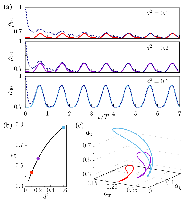
Figure 2: (color online) Periodically modulated continuous time quantum random walk of a qubit. Dynamics, spectral gap, and limit cycle solution for three values of the parameter $d^{2}$ of the amplitude damping map $\mathcal{E}_{1}$, see Eq. (12), are shown. $(a)$ Relaxation of the state $|0\rangle$ population obtained by numerical integration of Eq. (1) with initial condition $\rho(0)=|0\rangle\langle 0|$ (dotted lines), and asymptotic periodic states (solid lines) obtained from the Floquet propagator $\mathbf{U}_{T}$ of the embedded system. (b) Relevant spectral gap $g$ of $\mathbf{U}_{T}$. (c) Limit cycle solutions for the Bloch vector. The waiting time distribution (10) has parameters $\gamma=1$ and $A=0.24$. The modulation frequency $\Omega$ is $0.1$.

In Fig. 2(a) we show the time evolution of $\rho_{00}(t)=\langle 0|\rho(t)|0\rangle$ obtained by the direct integration of Eq. (1), starting from $\rho(0)=|0\rangle\langle 0|$ (dashed lines). After several periods, the solutions land on the asymptotic limit cycles (solid lines) obtained from the Floquet propagator $\mathbf{U}_{T}$ with three Arnoldi iterations. The corresponding limit cycles of the Bloch vector of components $a_{i}={\rm Tr}\{\rho\sigma_{i}\}$ ($i=x,y,z$) are presented in Fig. 2(c). As shown in Fig. 2(b), the relevant spectral gap increases with the value of $d^{2}$, which in turn corresponds to a shorter timescale of relaxation towards the asymptotic state, see dashed lines in Fig. 2(a).

IV Conclusions

We have presented a method to find the asymptotic Floquet states for a class of periodically modulated systems governed by memory-kernel master equations. The method has been applied to a time-periodically modulated model of piecewise dynamics of a qubit, a quantum generalization of a classical semi-Markov process Breuer2008 . The asymptotic Floquet states are especially interesting in this context. In the stationary limit, the difference in non-Markovian and Markovian evolutions is noticeable only during the relaxation towards the asymptotic stationary state Breuer et al. (2016), which, f.e., in the case of the qubit is a point inside (or on) Bloch sphere. This point can be reached by following infinitely many trajectories, some of them corresponding to Markovian evolution and some not, so once the relaxation is over it is impossible to decide what kind of evolution the system has undergone. It is different when the qubit is periodically modulated because its asymptotic state represents a one-dimensional, time-parametrized manifold; see Fig. 2(c). This manifold is specific to the Liouville superoperator $\mathcal{L}$ and it could be that some Floquet states are not attainable with Markovian $\mathcal{L}$. Outside of the quantum field, memristors Pershin and Di Ventra (2011) and meta-materials with memory Driscoll et al. (2009); Zheng et al. (2013) are considered now as perspective candidates for a new generation of nano-scale devices. They are typically modeled with equation (1); modulations can be introduced in these systems in different ways, thus creating room for new regimes.

Appendix A Derivation of Eq. (14)

Consider the general case in which the continuous background evolution between jumps is provided by some CPT map $\mathcal{F}(t)$. In the application we consider the case of a continuous time quantum random walk Budini (2004) by setting $\mathcal{F}(t)\equiv\mathbb{1}$. The jumps are caused by the instantaneous actions of a CPT map $\mathcal{E}(t)$ at random instances of time distributed according to a waiting time distribution $f(t)$. The starting point for deriving the generalized master equation (14) for the density matrix $\rho(t)$ in the case of modulated piecewise dynamics, meaning that the map $\mathcal{E}$ is is itself time-dependent, is the following sum over trajectories

$$\rho(t) = \mathcal{G}(t)\rho_{0}+\sum_{n=1}^{\infty}\int_{0}^{t}dt_{n}\dots\int_{0}^{t_{2}}dt_{1}\tilde{\mathcal{F}}(t-t_{n})\mathcal{E}(t_{n})$$ (17)

$$\times\dots\mathcal{E}(t_{2})\tilde{\mathcal{F}}(t_{2}-t_{1})\mathcal{E}(t_{1})\mathcal{G}(t_{1})\rho_{0}\;,$$

where

$$\mathcal{G}(t) = g(t)\mathcal{F}(t)$$

$$\tilde{\mathcal{F}}(t_{j+1}-t_{j}) = f(t_{j+1}-t_{j})\mathcal{F}(t_{j+1}-t_{j})\;.$$ (18)

Here the function $g(t)$ gives the probability that no jump has occurred up to time $t$ and is therefore defined by $g(t)=1-\int_{0}^{t}d\tau f(\tau)$.
In order to obtain the piecewise dynamics described by Eq. (17) in the form of a master equation, we start by evaluating the series order by order in the number $n$ of jupms, i.e., of actions of the map $\mathcal{E}$.

• Zero jumps ($n=0$)

  $$\rho^{(0)}(t)=\mathcal{G}(t)\rho_{0}\;.$$ (19)

• One jump ($n=1$)

  $$\rho^{(1)}(t) = \int_{0}^{t}dt_{1}\tilde{\mathcal{F}}(t-t_{1})\mathcal{E}(t_{1})\mathcal{G}(t_{1})\rho_{0}$$ (20)

  $$= \int_{0}^{t}dt_{1}\tilde{\mathcal{F}}(t-t_{1})\mathcal{E}(t_{1})\rho^{(0)}(t_{1})\;.$$

• Two jumps ($n=2$)

  $$\rho^{(2)}(t) = \int_{0}^{t}dt_{2}\int_{0}^{t_{2}}dt_{1}\tilde{\mathcal{F}}(t-t_{2})\mathcal{E}(t_{2})$$ (21)

  $$\quad\times\tilde{\mathcal{F}}(t_{2}-t_{1})\mathcal{E}(t_{1})\mathcal{G}(t_{1})\rho_{0}$$

  $$= \int_{0}^{t}dt_{2}\tilde{\mathcal{F}}(t-t_{2})\mathcal{E}(t_{2})$$

  $$\quad\times\int_{0}^{t_{2}}dt_{1}\tilde{\mathcal{F}}(t_{2}-t_{1})\mathcal{E}(t_{1})\rho^{(0)}(t_{1})$$

  $$= \int_{0}^{t}dt_{2}\tilde{\mathcal{F}}(t-t_{2})\mathcal{E}(t_{2})\rho^{(1)}(t_{2})\;,$$

and so on. We find the recursive relation

$$\rho^{(n)}(t) = \int_{0}^{t}dt^{\prime}\tilde{\mathcal{F}}(t-t^{\prime})\mathcal{E}(t^{\prime})\rho^{(n-1)}(t^{\prime}),\qquad(n\geq 1)$$

$$\rho^{(0)}(t) = \mathcal{G}(t)\rho_{0}\;.$$ (22)

Summing the series we get

$$\rho(t) = \mathcal{G}(t)\rho_{0}+\int_{0}^{t}dt^{\prime}\tilde{\mathcal{F}}(t-t^{\prime})\mathcal{E}(t^{\prime})\sum_{n=1}^{\infty}\rho^{(n-1)}(t^{\prime})$$ (23)

$$= \mathcal{G}(t)\rho_{0}+\int_{0}^{t}dt^{\prime}\tilde{\mathcal{F}}(t-t^{\prime})\mathcal{E}(t^{\prime})\rho(t^{\prime})\;.$$

Finally, taking the time derivative of Eq. (23) we obtain

$$\dot{\rho}(t) = \frac{d}{dt}\mathcal{G}(t)\rho_{0}+\int_{0}^{t}dt^{\prime}\frac{\partial}{\partial t}\tilde{\mathcal{F}}(t-t^{\prime})\mathcal{E}(t^{\prime})\rho(t^{\prime})$$ (24)

$$+\tilde{\mathcal{F}}(0)\mathcal{E}(t)\rho(t)$$

$$= \int_{0}^{t}dt^{\prime}\mathcal{K}(t-t^{\prime})\mathcal{E}(t^{\prime})\rho(t^{\prime})+\mathcal{I}(t)\rho_{0}\;,$$

where

$$\mathcal{K}(t) = \frac{d}{dt}\tilde{\mathcal{F}}(t)+\tilde{\mathcal{F}}(0)\delta(t)$$

$$\mathcal{I}(t) = \frac{d}{dt}\mathcal{G}(t)\;.$$ (25)

In the static case $\mathcal{E}(t)\equiv\mathcal{E}$, Eq. (24) coincides with Eq. (7) of Ref. Vacchini (2013). If instead we set $\mathcal{F}(t)\equiv\mathbb{1}$ the case considered in the application is recovered.

References

- (1) L. P. Kadanoff, From Order to Chaos (World Scientific, 1993).
- Petrov et al. (1997) V. Petrov, Q. Ouyang, and H. L. Swinney, Nature 388, 655 (1997).
- Herrmann (2001) C. S. Herrmann, Exp. Brain Res. 137, 346 (2001).
- Shirley (1965) J. H. Shirley, Phys. Rev. 138, B979 (1965).
- Sambe (1973) H. Sambe, Phys. Rev. A 7, 2203 (1973).
- Grifoni and Hänggi (1998) M. Grifoni and P. Hänggi, Phys. Rep. 304, 229 (1998).
- Bukov et al. (2015) M. Bukov, L. D’Alessio, and A. Polkovnikov, Adv. Phys. 64, 139 (2015).
- Eckardt and Anisimovas (2015) A. Eckardt and E. Anisimovas, New J. Phys. 17, 093039 (2015).
- Lindner et al. (2011) N. H. Lindner, G. Refael, and V. Galitski, Nat. Phys. 7, 490 (2011).
- Liu et al. (2013) D. E. Liu, A. Levchenko, and H. U. Baranger, Phys. Rev. Lett. 111, 047002 (2013).
- Struck et al. (2011) J. Struck, C. Ölschläger, R. Le Targat, P. Soltan-Panahi, A. Eckardt, M. Lewenstein, P. Windpassinger, and K. Sengstock, Science 333, 996 (2011).
- Goldman and Dalibard (2014) N. Goldman and J. Dalibard, Phys. Rev. X 4, 031027 (2014).
- Else et al. (2016) D. V. Else, B. Bauer, and C. Nayak, Phys. Rev. Lett. 117, 090402 (2016).
- Zhang et al. (2017) J. Zhang et al., Nature 543, 217 (2017).
- Choi et al. (2017) S. Choi et al., Nature 543, 221 (2017).
- Floquet (1883) G. Floquet, Ann. Sci. Ec. Norm. Sup. 12, 47 (1883).
- Yakubovich and Starzhinskii (1975) V. A. Yakubovich and V. M. Starzhinskii, Linear Differential Equations with Periodic Coeffcients (Wiley, New York, 1975).
- Jung (1993) P. Jung, Phys. Rep. 234, 175 (1993).
- Gammaitoni et al. (1998) L. Gammaitoni, P. Hänggi, P. Jung, and F. Marchesoni, Rev. Mod. Phys. 70, 223 (1998).
- Hartmann et al. (2017) M. Hartmann, D. Poletti, M. Ivanchenko, S. Denisov, and P. Hänggi, New J. Phys. 19, 083011 (2017).
- Vorberg et al. (2013) D. Vorberg, W. Wustmann, R. Ketzmerick, and A. Eckardt, Phys. Rev. Lett. 111, 240405 (2013).
- Lazarides and Moessner (2017) A. Lazarides and R. Moessner, arXiv:1703.02547 (2017).
- Sommer and Simon (2016) A. Sommer and J. Simon, New J. Phys. 18, 035008 (2016).
- Meinert et al. (2016) F. Meinert, M. J. Mark, K. Lauber, A. J. Daley, and H. C. Nägerl, Phys. Rev. Lett. 116, 205301 (2016).
- Eckardt (2017) A. Eckardt, Rev. Mod. Phys. 89, 011004 (2017).
- Kohler et al. (2005) S. Kohler, J. Lehmann, and P. Hänggi, Phys. Rep. 406, 379 (2005).
- Alicki and Lendi (2007) R. Alicki and K. Lendi, Quantum Dynamical Semigroups and Applications, Lecture Notes in Physics, Vol. 717 (Springer Berlin Heidelberg, 2007).
- Bastidas et al. (2017) V. M. Bastidas, T. H. Kyaw, J. Tangpanitanon, G. Romero, L.-C. Kwek, and D. G. Angelakis, arXiv:1707.04423v1 (2017).
- Breuer et al. (2016) H.-P. Breuer, E.-M. Laine, J. Piilo, and B. Vacchini, Rev. Mod. Phys. 88, 021002 (2016).
- (30) Bi-Heng Liu, Li Li, Yun-Feng Huang, Chuan-Feng Li, Guang-Can Guo, E.-M.Laine, H.-P. Breuer, J. Piilo, Nature Phys. 7, 931 (2011).
- Traversa et al. (2013) F. L. Traversa, M. Di Ventra, and F. Bonani, Phys. Rev. Lett. 110, 170602 (2013).
- Budini (2004) A. A. Budini, Phys. Rev. A 69, 042107 (2004).
- Note (1) For , the method has to be complemented with a non-homogeneous extension of Floquet theory Yakubovich and Starzhinskii (1975).
- Vacchini (2013) B. Vacchini, Phys. Rev. A 87, 030101 (2013).
- Vacchini (2016) B. Vacchini, Phys. Rev. Lett. 117, 230401 (2016).
- (36) Being preconditioned by the existence of the unique -periodic asymptotic solution , Eq. (1) can be transformed into the finite-length memory form used in Ref. Traversa et al. (2013), with , by folding the kernel into the time interval , , and setting .
- Grabert et al. (1977) H. Grabert, P. Talkner, and P. Hänggi, Z. Physik B 26, 389 (1977).
- Grabert et al. (1978) H. Grabert, P. Talkner, and P. Hänggi, Z. Physik B 29, 273 (1978).
- Grabert et al. (1980) H. Grabert, P. Hänggi, and P. Talkner, J. Stat. Phys. 22, 537 (1980).
- Grigolini (1982) P. Grigolini, J. Stat. Phys. 27, 283 (1982).
- Kupferman (2004) R. Kupferman, J. Stat. Phys. 114, 291 (2004).
- Siegle et al. (2010) P. Siegle, I. Goychuk, P. Talkner, and P. Hänggi, Phys. Rev. E 81, 011136 (2010).
- Cox and Miller (1977) D. Cox and H. Miller, The Theory of Stochastic Processes (Chapman and Hall/CRC, 1977).
- Breuer (2004) H.-P. Breuer, Phys. Rev. A 70, 012106 (2004).
- Budini (2013) A. A. Budini, Phys. Rev. A 88, 032115 (2013).
- Kretschmer et al. (2016) S. Kretschmer, K. Luoma, and W. T. Strunz, Phys. Rev. A 94, 012106 (2016).
- (47) H.-P. Breuer and B. Vacchini, Phys. Rev. Lett. 101, 140402 (2008).
- Cox (1955) D. R. Cox, Math. Proc. Cambridge 51, 433 (1955).
- Beylkin and Monzón (2005) G. Beylkin and L. Monzón, Appl. Comput. Harmon. Anal. 19, 17 (2005).
- Levin et al. (2008) D. Levin, Y. Peres, and E. Wilmer, Markov Chains and Mixing Times, 1st ed. (American Mathematical Society, 2008).
- Golub and Van Loan (1996) G. H. Golub and C. F. Van Loan, Matrix Computations, 3rd ed., Vol. 3 (The Johns Hopkins University Press, Baltimore, 1996).
- Vacchini (2012) B. Vacchini, J. Phys. B 45, 154007 (2012).
- Nielsen and Chuang (2010) M. A. Nielsen and I. L. Chuang, Quantum Computation and Quantum Information (Cambridge University Press, NY, 2010).
- Grifoni et al. (1996) M. Grifoni, M. Sassetti, and U. Weiss, Phys. Rev. E 53, R2033 (1996).
- Pershin and Di Ventra (2011) Y. V. Pershin and M. Di Ventra, Adv. Phys. 60, 145 (2011).
- Driscoll et al. (2009) T. Driscoll, H.-T. Kim, B.-G. Chae, B.-J. Kim, Y.-W. Lee, N. M. Jokerst, S. Palit, D. R. Smith, M. Di Ventra, and D. N. Basov, Science 325, 1518 (2009).
- Zheng et al. (2013) X. Zheng, Y. Yan, and M. Di Ventra, Phys. Rev. Lett. 111, 086601 (2013).