Light-nuclei spectra from chiral dynamics

A major goal of nuclear theory is to explain the spectra and stability of nuclei in terms of effective many-body interactions amongst the nucleus’ constituents—the nucleons, i.e., protons and neutrons. Such an approach, referred to below as the basic model of nuclear theory, is formulated in terms of point-like nucleons, which emerge as effective degrees of freedom, at sufficiently low energy, as a result of a decimation process, starting from the fundamental quarks and gluons, described by Quantum Chromodynamics (QCD). A systematic way to account for the constraints imposed by the symmetries of QCD, in particular chiral symmetry, is provided by chiral effective field theory, in the framework of a low-energy expansion. Here we show, in quantum Monte Carlo calculations accurate to $\leq\!2\%$ of the binding energy, that two- and three-body chiral interactions fitted only to bound- and scattering-state observables in, respectively, the two- and three-nucleon sectors, lead to predictions for the energy levels and level ordering of nuclei in the mass range $A\,$= 4–12 in very satisfactory agreement with experimental data. Our findings provide strong support for the fundamental assumptions of the basic model, and pave the way to its systematic application to the electroweak structure and response of these systems as well as to more complex nuclei.

The nuclear Hamiltonian in the basic model is taken to consist of non-relativistic kinetic energy, and two- and three-body interactions. There are indications that four-body interactions may contribute at the level of $\sim\,$100 keV in ⁴He, but current formulations of the basic model do not typically include them (see, for example, Ref. Carlson:2015 ). Two-body interactions consist of a long-range component, for inter-nucleon separation $r\gtrsim 2$ fm, due to one-pion exchange (OPE) Yukawa:1935 , and intermediate- and short-range components, for, respectively, $1\,\,{\rm fm}\lesssim r\lesssim 2$ fm and $r\lesssim 1$ fm. Up to the mid-1990’s, such models were based almost exclusively on meson-exchange phenomenology. The mid-1990’s models Stoks:1994 ; Wiringa:1995 ; Machleidt:2001 were constrained by fitting nucleon-nucleon ($N\!N$) elastic scattering data up to lab energies of 350 MeV, with $\chi^{2}$/datum $\simeq 1$ relative to the database available at the time Stoks:1993 . Two well-known and still widely used examples in this class are the Argonne $v_{18}$ (AV18) Wiringa:1995 and CD-Bonn Machleidt:2001 . These so-called realistic interactions also contained isospin-symmetry-breaking (ISB) terms. At the level of accuracy required Stoks:1993 , full electromagnetic interactions, along with strong interactions, had to be specified in order to fit the data precisely, and the AV18 model included electromagnetic corrections up to order $\alpha^{2}$ ($\alpha$ is the fine structure constant).

Already in the 1980’s, accurate three-body calculations showed that contemporary $N\!N$ interactions did not provide enough binding for the three-body nuclei, ³H and ³He Friar:1984 . In the late 1990’s and early 2000’s this realization was extended to the spectra (ground and low-lying excited states) of light p-shell nuclei in calculations based on quantum Monte Carlo (QMC) methods Pudliner:1997 and in no-core shell-model (NCSM) studies Navratil:2000 . Consequently, the basic model with $N\!N$ interactions fit to scattering data, without the inclusion of a three-nucleon ($3N$) interaction, is incomplete.

Because of the composite nature of the nucleon and, in particular, the dominant role of the $\Delta$ resonance in pion-nucleon scattering, multi-nucleon interactions arise quite naturally in meson-exchange phenomenology. The Illinois $3N$ interactions Pieper:2001 contain a dominant two-pion exchange (TPE)—the venerable Fujita-Miyazawa interaction Fujita:1957 —and smaller multi-pion exchange components resulting from the excitation of intermediate $\Delta$’s. The most recent version, Illinois-7 (IL7) Pieper:2008 , also contains phenomenological isospin-dependent central terms. The small number (four) of parameters that fully characterize it were determined, in conjunction with the AV18, by fitting 23 ground or low-lying nuclear states in the mass range $A$=3–10. The resulting AV18+IL7 Hamiltonian then led to predictions of about 100 ground- and excited-state energies up to $A$=12, including the ¹²C ground- and Hoyle-state energies, in good agreement with the corresponding empirical values Carlson:2015 .

A new phase in the evolution of the basic model, and renewed interest in its further development, have been spurred by the emergence in the early 1990’s of chiral effective field theory ($\chi$EFT) Weinberg:1990 ; Weinberg:1991 ; Weinberg:1992 . In $\chi$EFT the symmetries of QCD, in particular its approximate chiral symmetry, are used to systematically constrain classes of Lagrangians describing, at low energies, the interactions of baryons ($N$’s and $\Delta$’s) with pions as well as the interactions of these hadrons with electroweak fields Park:1993 ; Park:1996 ; Park:2003 . While the conventional meson-exchange formulation of the basic model described earlier relied on an expansion in terms of exchanges of heavier and heavier mesons (and hence shorter and shorter ranges of associated interactions), the $\chi$EFT formulation has, by contrast, an expansion in powers of pion momenta as its organizing principle, directly rooted in QCD. From this perspective, it can be justifiably argued to have put the basic model on a more fundamental basis, by providing a link between QCD and its symmetries, and the strong and electroweak interactions in nuclei.

Within $\chi$EFT many studies have been carried out dealing with the construction of $NN$ and $3N$ interactions Ordonez:1996 ; Epelbaum:1998 ; Entem:2003 ; Machleidt:2011 ; vanKolck:1994 ; Epelbaum:2002 ; Bernard:2011 ; Girlanda:2011 ; Krebs:2012 and accompanying ISB corrections Friar:1999 ; Friar:2004 ; Friar:2005 . These interactions were typically formulated in momentum space, and included cutoff functions to regularize their behavior at large momenta which, however, made them strongly non-local when Fourier-transformed in configuration space, and therefore unsuitable for use with quantum Monte Carlo methods Carlson:2015 . Among these, in particular, Green’s Function Monte Carlo (GFMC) is the method of choice to provide reliable solutions of the many-body Schrödinger equation—presently for up to $A\,$=12 nucleons—with full account of the complexity of the many-body, spin- and isospin-dependent correlations induced by nuclear interactions.

Nuclear Hamiltonian

In order to overcome these difficulties, in recent years local, configuration-space chiral $NN$ interactions have been derived Gezerlis:2013 ; Piarulli:2016 . We will point out differences between these models below. In the following, we focus on the family of local interactions constructed by our group. They are written as the sum of an electromagnetic-interaction component, $v^{\rm EM}_{ij}$, including first- and second-order Coulomb, Darwin-Foldy, vacuum polarization, and magnetic moment terms (as in Ref. Wiringa:1995 ), and a strong-interaction component, $v_{ij}$, characterized by long- and short-range parts Piarulli:2016 . The long-range part includes OPE and TPE terms up to next-to-next-to-leading order (N2LO) in the chiral expansion Piarulli:2015 , derived in the static limit from leading and sub-leading $\pi N$ and $\pi N\Delta$ chiral Lagrangians. Its strength is fully determined by the nucleon and nucleon-to-$\Delta$ axial coupling constants $g_{A}$ and $h_{A}$, the pion decay amplitude $f_{\pi}$, and the sub-leading low-energy constants (LECs, in standard notation) $c_{1}$, $c_{2}$, $c_{3}$, $c_{4}$, and $b_{3}+b_{8}$ constrained by reproducing $\pi N$ scattering data. In coordinate space, this long-range part is represented by charge-independent central, spin, and tensor components with and without isospin dependence ${\bm{\tau}}_{i}\cdot{\bm{\tau}}_{j}$ (the so-called $v_{6}$ operator structure), and by charge-independence-breaking central and tensor components induced by OPE and proportional to the isotensor operator $T_{ij}\,$=$\,3\,\tau^{z}_{i}\,\tau^{z}_{j}-{\bm{\tau}}_{i}\cdot{\bm{\tau}}_{j}$. The radial functions multiplying these operators are singular at the origin (they behave as $1/r^{n}$ with $n$ taking on values up to $n\,$=$\,6$), and are regularized by a cutoff of the form Piarulli:2015

$$C_{R_{\rm L}}(r)=1-\frac{1}{(r/R_{\rm L})^{6}\,{\rm e}^{(r-R_{\rm L})/a_{\rm L}}+1}\ ,$$ (1)

with $a_{\rm L}$ taken as $R_{\rm L}/2$, and the values for $R_{\rm L}$ considered here are given below.

The short-range part is described by charge-independent contact interactions, specified by a total of 20 LECs—2 at LO, 7 at NLO, and 11 at next-to-next-to-next-to-leading (N3LO)—and charge-dependent ones characterized by 6 LECs—2 at LO, one each from charge-independence-breaking and charge-symmetry-breaking (proportional, respectively, to $T_{ij}$ and $\tau^{z}_{i}+\tau^{z}_{j}$), and 4 at NLO from charge-independence-breaking Piarulli:2016 . In the NLO and N3LO contact interactions, Fierz transformations have been utilized to rearrange terms that in configuration space would otherwise lead to powers of ${\bf p}$—the relative momentum operator—higher than two. The resulting charge-independent interaction contains, in addition to the $v_{6}$ operator structure, spin-orbit, ${\bf L}^{2}$ (${\bf L}$ is the relative orbital angular momentum), and quadratic spin-orbit components, while the charge-dependent one retains central, tensor, and spin-orbit components. Both are regularized by multiplication of a Gaussian cutoff,

$$C_{R_{\rm S}}(r) = \frac{1}{\pi^{3/2}\,R_{\rm S}^{3}}{\rm e}^{-(r/R_{\rm S})^{2}}\ .$$ (2)

These 26 LECs in the short-range part of $v_{ij}$ were constrained by a fit to the $NN$ database, including the deuteron ground-state energy and two-neutron scattering length, as assembled by the Granada group Perez:2013 . Two classes of interactions were constructed, which only differ in the range of laboratory energy over which the fits were carried out, either 0–125 MeV in class I or 0–200 MeV in class II. For each class, three different sets of cutoff radii $(R_{\rm S},R_{\rm L})$ were considered $(R_{\rm S},R_{\rm L})\,$=$\,(0.8,1.2)$ fm in set a, (0.7,1.0) fm in set b, and (0.6,0.8) fm in set c. The $\chi^{2}$/datum achieved by the fits in class I (II) was $\lesssim 1.1(\lesssim 1.4)$ for a total of about 2700 (3700) data points. We will refer to these high-quality $NN$ interactions generically as the Norfolk $v_{ij}$’s (NV2s), and designate those in class I as NV2-Ia, NV2-Ib, and NV2-Ic, and those in class II as NV2-IIa, NV2-IIb, and NV2-IIc.

We observe that the models of Ref. Gezerlis:2013 do not include $\Delta$ contributions and only retain contact interactions up to NLO for a total of 9 LECs. These LECs were fitted to the phase-shifts of the Nijmegen partial-wave analysis Stoks:1993 , rather than to its database of $NN$ cross sections and polarization observables. Some of the drawbacks that this entails are discussed in Ref. Piarulli:2015 .

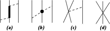
Figure 1: $3N$ chiral interaction. Diagrams illustrating schematically the contributions to the $3N$ interaction. Nucleons, $\Delta$’s, and pions are denoted by solid, thick-solid, and dashed lines, respectively. The circle in panel (b) represents the vertex involving the LECs $c_{1}$, $c_{3}$, and $c_{4}$ in ${\cal L}^{(2)}_{\pi N}$.

The NV2s were found to provide insufficient attraction, in GFMC calculations, for the ground-state energies of nuclei with $A\,$=$\,3$–6 Piarulli:2016 ; Lynn:2016 ; Lynn:2017 , thus corroborating the insight realized in the early 2000’s within the older (and less fundamental) meson-exchange phenomenology. To remedy this shortcoming, we construct here the leading $3N$ interaction $V_{ijk}$ in $\chi$EFT, including $\Delta$ intermediate states. It is illustrated diagrammatically in Fig. 1, and consists vanKolck:1994 ; Epelbaum:2002 of a long-range piece mediated by TPE and denoted with the superscript $2\pi$, panels (a) and (b), and a short-range piece parametrized in terms of three contact interactions and denoted with the superscript CT, panels (c) and (d),

$$V_{ijk}=\sum_{{\rm cyclic}\,\,ijk}\left(\,V^{2\pi}_{ijk}+V^{\rm CT}_{ijk}\,\right)\ .$$ (3)

In configuration space, the TPE term from intermediate $\Delta$ states, panel (a) in Fig. 1, and from interactions proportional to the LECs $c_{1}$, $c_{3}$, and $c_{4}$ in the sub-leading chiral Lagrangian ${\cal L}^{(2)}_{\pi N}$ Fettes:2000 , panel (b), reads

$$V^{2\pi}_{ijk} = \frac{g_{A}^{2}}{256\,\pi^{2}}\frac{m_{\pi}^{6}}{f_{\pi}^{4}}\Big{[}8\,c_{1}\,\Sigma_{ij}\,\Sigma_{kj}\,\mathcal{T}^{\,(+)}_{ijk}+\,\frac{2}{9}\,\widetilde{c}_{3}\,\Sigma^{(+)}_{ijk}\,\,\mathcal{T}^{\,(+)}_{ijk}$$ (4)

$$-\frac{1}{9}\Big{(}\widetilde{c}_{4}+\frac{1}{4\,m}\Big{)}\Sigma^{(-)}_{ijk}\,\,\mathcal{T}^{\,(-)}_{ijk}\Big{]}\ ,$$

with spin and isospin operator structures defined, respectively, as $\Sigma_{lm}\equiv\widetilde{Z}_{\pi}(r_{lm})\,{\bm{\sigma}}_{l}\cdot\hat{\bf r}_{lm}$, where ${\bf r}_{lm}\equiv{\bf r}_{l}-{\bf r}_{m}$, and

$$\Sigma^{(\mp)}_{ijk}\equiv\left[\widetilde{X}_{ij}\,,\,\widetilde{X}_{jk}\right]_{\mp},\,\,\,\,\mathcal{T}^{\,(\mp)}_{ijk}\equiv\left[{\bm{\tau}}_{i}\cdot{\bm{\tau}}_{j}\,,\,{\bm{\tau}}_{j}\cdot{\bm{\tau}}_{k}\right]_{\mp},$$ (5)

$$\qquad\widetilde{X}_{ij}\equiv\widetilde{T}_{\pi}(r_{ij})\,S_{ij}+\widetilde{Y}_{\pi}(r_{ij})\,{\bm{\sigma}}_{i}\cdot{\bm{\sigma}}_{j}\ .$$ (6)

Here $\left[\,\dots\,,\,\dots\right]_{\mp}$ denote commutators ($-$) or anti-commutators ($+$), $S_{ij}$ is the standard tensor operator, ${\bm{\sigma}}_{i}$ and ${\bm{\tau}}_{i}$ are Pauli spin and isospin matrices relative to nucleon $i$, and the regularized radial functions are defined as

$$\widetilde{Y}_{\pi}(r) = \frac{e^{-{m_{\pi}}r}}{{m_{\pi}}r}\,C_{R_{\rm L}}(r)\ ,$$ (7)

$$\widetilde{T}_{\pi}(r) = \left(1+\frac{3}{m_{\pi}\,r}+\frac{3}{m_{\pi}^{2}\,r^{2}}\right)\widetilde{Y}_{\pi}(r)\ ,$$ (8)

$$\widetilde{Z}_{\pi}(r) = -\left(1+\frac{1}{m_{\pi}\,r}\right)\widetilde{Y}_{\pi}(r)\ ,$$ (9)

where the cutoff $C_{R_{\rm L}}(r)$ is defined in Eq. (1). Lastly, the LECs $\widetilde{c}_{3}$ and $\widetilde{c}_{4}$ are related to the corresponding $c_{3}$ and $c_{4}$ in ${\cal L}^{(2)}_{\pi N}$ via

$$\widetilde{c}_{3}=c_{3}-\frac{h^{2}_{A}}{9\,m_{\Delta N}}\ ,\qquad\widetilde{c}_{4}=c_{4}+\frac{h^{2}_{A}}{18\,m_{\Delta N}}\ ,$$ (10)

where $h_{A}$ and $m_{\Delta N}$ are, respectively, the $N$-to-$\Delta$ axial coupling constant and $\Delta$-$N$ mass difference. The values of these constants as well as the LECs $c_{1}$, $c_{3}$, and $c_{4}$, the (average) pion mass $m_{\pi}$ and decay amplitude $f_{\pi}$, and (average) nucleon mass $m$ and axial coupling constant $g_{A}$, are taken from Tables I and II of Ref. Piarulli:2015 .

The CT term is parametrized as

$$V^{\rm CT}_{ijk} = \frac{g_{A}\,c_{D}}{96\,\pi}\,\frac{m_{\pi}^{3}}{\Lambda_{\chi}\,f_{\pi}^{4}}\,{\bm{\tau}}_{i}\cdot{\bm{\tau}}_{k}\,\widetilde{X}_{ik}\,\left[\,C_{R_{\rm S}}(r_{ij})+C_{R_{\rm S}}(r_{jk})\,\right]$$ (11)

$$+\frac{c_{E}}{\Lambda_{\chi}\,f_{\pi}^{4}}\,{\bm{\tau}}_{i}\cdot{\bm{\tau}}_{k}\,C_{R_{\rm S}}(r_{ij})\,C_{R_{\rm S}}(r_{jk})\ ,$$

where $C_{R_{\rm S}}(r)$ is the cutoff in Eq. (2), $\Lambda_{\chi}\,$ is the chiral-symmetry-breaking scale taken as $\Lambda_{\chi}\,$=$\,1$ GeV, and the two (adimensional) LECs $c_{D}$ and $c_{E}$ are determined by simultaneously reproducing the experimental ³H ground-state energy, $E_{0}(^{3}$H), and the neutron-deuteron ($nd$) doublet scattering length, ${}^{2}a_{nd}$. These observables are calculated with hyperspherical-harmonics (HH) expansion methods. By now, these variational methods have achieved a high degree of sophistication (see below, and for a more extended recent review Ref. Kievsky:2008 ), permitting the accurate, virtually exact solution of the bound- and scattering-state problem—the latter, both below and above two-body breakup thresholds—in the three- and four-nucleon systems.

The determination of $c_{D}$ and $c_{E}$ proceeds as follows. For a range of $c_{D}$ values we determine $c_{E}$ by reproducing either $E_{0}(^{3}$H) or ${}^{2}a_{nd}$ (its central value). The intercept of the resulting trajectories in the $(c_{D},c_{E})$-plane provides the sought simultaneous solution. This procedure is repeated for each NV2-I(a-b) and NV2-II(a-b) with the cutoff radii $(R_{\rm S},R_{\rm L})$ in the Norfolk $3N$ interactions matching those of the corresponding NV2s to make the NV2+3 models reported here; the $c_{D},c_{E}$ values for each combination are listed in Table 1. We observe that models NV2-Ic and NV2-IIc are not considered any further in the present work, owing to the difficulty in the convergence of the HH expansion and the severe fermion-sign problem in the GFMC imaginary-time propagation with these interactions Piarulli:2016 .

Table 1: Fitted values of $c_{D}$ and $c_{E}$ and HH results for $A\,$= 3–4 observables. The (adimensional) values of $c_{D}$ and $c_{E}$ obtained for the different NV2+3 chiral interactions having cutoff radii $(R_{\rm S},R_{\rm L})$ equal to (0.8,1.2) fm for models Ia and IIa, and (0.7,1.0) fm for models Ib and IIb are shown along with the ³H, ³He, and ⁴He ground-state energies (in MeV) and $nd$ doublet scattering length (in fm), obtained in HH calculations without and with the inclusion of the three-body interactions; the experimental values are $E_{0}(^{3}$H) = –8.482 MeV, $E_{0}(^{3}$He) = –7.718 MeV, $E_{0}(^{4}$He) = –28.30 MeV, and ${}^{2}a_{nd}\,$=$\,(0.645\pm 0.010)$ fm. The $E_{0}(^{3}$H) and ${}^{2}a_{nd}$ observables are fitted when $3N$ interactions are included.

			w/o $3N$				with $3N$
Model	$c_{D}$	$c_{E}$	$E_{0}(^{3}$H)	$E_{0}(^{3}$He)	$E_{0}(^{4}$He)	${}^{2}a_{nd}$	$E_{0}(^{3}$He)	$E_{0}(^{4}$He)
Ia	3.666	–1.638	–7.825	–7.083	–25.15	1.085	–7.728	–28.31
Ib	–2.061	–0.982	–7.606	–6.878	–23.99	1.284	–7.730	–28.31
IIa	1.278	–1.029	–7.956	–7.206	–25.80	0.993	–7.723	–28.17
IIb	–4.480	–0.412	–7.874	–7.126	–25.31	1.073	–7.720	–28.17

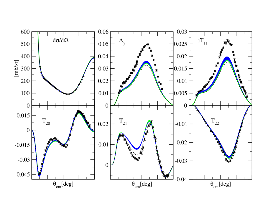
Figure 2: Polarization observables in $pd$ elastic scattering at 3 MeV. Polarization observables obtained in HH calculations with the NV2+3 models Ia-Ib (IIa-IIb) are shown by the green (blue) band. Also shown by the black dashed line are results obtained with only the two-body interaction NV2-Ia.

In Table 1 we also report the $nd$ scattering length and ground-state energies of ³H, ³He, and ⁴He obtained without $3N$ interaction as well as those predicted for ³He and ⁴He when this interaction is included (experimental values for the scattering length and energies are taken, respectively, from Ref. Schoen:2003 and Ref. Audi:2003 ). Increasing the laboratory-energy range over which the $NN$ interaction is fitted, from 0–125 MeV in class I to 0–200 MeV in class II, decreases the $A\,$= 3–4 ground-state energies calculated without the $3N$ interaction, by as much as 1.3 MeV in ⁴He with model b. However, when the $3N$ interaction is included, the effect is reversed and much reduced, in ⁴He the increase amounts to 140 keV in going from model Ib to IIb. The dependence on the cutoff radii $(R_{\rm S},R_{\rm L})$, i.e., the difference between the rows Ia-Ib and IIa-IIb, is significant without the $3N$ interaction, but turns out to be negligible when it is retained, being in this case of the order of a few keV and hence comparable to the numerical precision of the present HH methods. This tradeoff is of course achieved through the large variation of the LECs $c_{D}$ and $c_{E}$, which remain nevertheless of natural order in both models, a and b.

In Fig. 2 the differential cross section, and vector and tensor polarization observables in proton-deuteron elastic scattering obtained with the present NV2+3 models are compared to experimental data Shimizu:1995 . Theoretical predictions remain essentially unchanged for Ia-Ib, but display a small variation for IIa-IIb, as the cutoff radii $(R_{\rm S},R_{\rm L})$ are reduced from (0.8,1.2) fm in models a to (0.7,1.0) fm in models b. The effect of the $3N$ interaction is small, marginally improving (appreciably worsening) the agreement between theory and experiment for the observables $A_{y}$, $i\,T_{11}$, and $T_{22}$ ($T_{20}$ and $T_{21}$). In particular, the well known discrepancy in the vector analyzing power—the “$A_{y}$ puzzle” Gloeckle:1996 —persists. It also appears to be unresolved when higher-order chiral loops are accounted for in the long-range component of the $3N$ interaction Golak:2014 . Subleading contact terms in its short-range component, while having been formally derived Girlanda:2011 , have yet to be implemented in calculations, since they depend on 10 unknown LECs. Indeed, members of the present collaboration are currently involved in a fit of these LECs to experimental data on $3N$ scattering observables.

Hyperspherical-harmonics expansion method

The HH method uses hyperspherical-harmonics functions as an expansion basis for the wave function of an $A$-body system Kievsky:2008 . In the specific case of $A\,$=$\,3$ and 4 nuclei, the bound-state wave function $\Psi_{A}$, having total angular momentum and parity quantum numbers $J^{\pi}$, is expanded as

$$\Psi_{A}=\sum_{[K_{A}]}u_{[K_{A}]}(\rho_{A}){\cal B}_{[K_{A}]}(\Omega_{A})\ ,$$ (12)

where ${\cal B}_{[K_{A}]}(\Omega_{A})$ are fully antisymmetrized HH-spin-isospin functions, which for three and four nucleons are characterized, respectively, by the set of quantum numbers $[K_{3}]\equiv[n_{1},l_{1},l_{2},L,s,S,t,T]$ and $[K_{4}]\equiv[n_{1},n_{2},l_{1},l_{2},l_{3},l^{\prime},L,s,s^{\prime},S,t,t^{\prime},T]$. The quantum numbers $n_{i},l_{i}$ and $l^{\prime}$ enter in the construction of the HH vector and are such that the grand angular momenta are $K_{3}=2\,n_{1}+l_{1}+l_{2}$ and $K_{4}=2\,n_{1}+2\,n_{2}+l_{1}+l_{2}+l_{3}$. The orbital angular momenta $l_{i}$ (and $l^{\prime}$ for $A=4$) are coupled to give the total orbital angular momentum $L$. The total spin and isospin of the vector are indicated, respectively, by $S$ and $T$, and $s,s^{\prime},t,t^{\prime}$ denote intermediate couplings.

The hyperspherical coordinates $(\rho_{A},\Omega_{A})$ in Eq. (12) are given by the hyperradius $\rho_{A}=(\sum_{i=1}^{A-1}{\bf x}_{i}^{2})^{1/2}$ expressed in terms of the $A$–$1$ Jacobi vectors ${\bf x}_{i}$ of the systems, and the hyperangles $\Omega_{A}=({\hat{\bf x}}_{1}\ldots{\hat{\bf x}}_{A-1},\alpha_{2}\ldots\alpha_{A-1})$, with ${\hat{\bf{x}}}_{i}$ being the unit Jacobi vectors and $\alpha_{i}$ the hyperangular variables. In the present application, the hyperradial functions are expanded in terms of generalized Laguerre polynomials multiplied by an exponential function

$$u_{\mu}(\rho_{A})=\sum_{m}C_{m,\mu}\;{\cal L}_{m}^{(3A-4)}(z)\;e^{-z/2}\ ,$$ (13)

with $z=\beta\rho_{A}$, $\beta$ being a nonlinear parameter and $\mu\equiv[K_{A}]$. After introducing the above expansion in Eq. (12), the wave function $\Psi_{A}$ is expressed compactly as

$$\Psi_{A} = \sum_{m,\mu}C_{m,\mu}\;\Phi_{m,\mu}(\rho_{A},\Omega_{A})\ ,$$ (14)

$$\Phi_{m,\mu}(\rho_{A},\Omega_{A}) = {\cal L}_{m}^{(3A-4)}(z)e^{-z/2}{\cal B}_{[K_{A}]}(\Omega_{A})\ ,$$ (15)

where the $\Phi_{m,\mu}(\rho_{A},\Omega_{A})$’s form a complete basis.

The ground-state energy $E_{0}$ follows from the Rayleigh-Ritz variational principle. This leads to a generalized eigenvalue problem, which is then solved with standard numerical techniques Kievsky:2008 . The convergence of the energy $E_{0}$ is studied in terms of the size of the basis. For the three-nucleon system ($J^{\pi}\,$= 1/2⁺) all possible combinations of HH functions up to $l_{1}+l_{2}\,$= 6 and isospin components $T\,$= 1/2 and 3/2 have been taken into account, thus attaining a level of accuracy of the order of a few keV on the sought energy eigenvalue. For $A\,$=$\,4$ ($J^{\pi}\,$= 0⁺), all possible combinations of HH functions up to $l_{1}+l_{2}+l_{3}\,$= 6 ($l_{1}+l_{2}+l_{3}\,$= 2) having $T\,$= 0 ($T\,$= 1 and 2) have been considered, attaining in this case a level of accuracy of about 20 keV for the ⁴He ground state energy Viviani:2005 .

The $J\,$= 1/2⁺ $nd$ scattering wave function $\Psi_{nd}$, used to calculate the doublet $nd$ scattering length, is expressed as $\Psi_{nd}=\Psi_{C}+\Phi_{nd}$, and $\Psi_{C}$ vanishes in the limit of large $nd$ separation. It is expanded in terms of HH function and Laguerre polynomials as for the bound state, using Eq. (14). The wave function $\Phi_{nd}$ describes the system in the asymptotic region

$$\Phi_{nd} = \sum_{{\rm cyclic}\,ijk}\sum_{L^{\prime}S^{\prime}}[[s_{i}\otimes\phi_{d}(jk)]_{S^{\prime}}\otimes Y_{L^{\prime}}({\hat{\bf{r}}_{nd}})]_{JJ_{z}}$$ (16)

$$\times[\delta_{LL^{\prime}}\delta_{SS^{\prime}}j_{L^{\prime}}(pr_{nd})+^{J}\!\!R_{LS}^{L^{\prime}S^{\prime}}(p)n_{L^{\prime}}(pr_{nd})g(pr_{nd})]\ ,$$

where $\phi_{d}$ is the deuteron wave function, $p$ ($r_{nd}$) is the $nd$ relative momentum (distance), and $j_{L}$ ($n_{L}$) are the regular (irregular) Bessel functions. The function $g(pr_{nd})$ modifies $n_{L}$ at small $r_{nd}$ by regularizing it at the origin, and $g(pr_{nd})\rightarrow 1$ for $r_{nd}\geq 10$ fm. Finally, the real parameters ${}^{J}R_{LS}^{L^{\prime}S^{\prime}}(p)$ are the $R$-matrix elements which determine phase shifts and, for coupled channels, mixing angles.

The unknown quantities in $\Psi_{nd}$, i.e., the coefficients $C_{m,\mu}$ in the expansion of $\Psi_{C}$ and $R$-matrix elements ${}^{J}R_{LS}^{L^{\prime}S^{\prime}}(p)$ in $\Phi_{nd}$, are obtained by utilizing the Kohn variational principle, which leads to a set of inhomogeneous coupled equations for $C_{m,\mu}$ and a set of algebraic equations for ${}^{J}R_{LS}^{L^{\prime}S^{\prime}}(p)$, solved by standard techniques Kievsky:2008 . In particular, the $nd$ doublet scattering length simply follows from ${}^{2}a_{nd}=-\lim_{p\rightarrow 0}{{}^{1/2}R_{0\,1/2}^{0\,1/2}(p)}$, and the convergence of the HH expansion for ${}^{2}a_{nd}$ is established with a procedure similar to that outlined above for the bound state, ultimately achieving an accuracy of the order of 0.001 fm. The extension of the method to describe proton-deuteron scattering, specifically the inclusion, in the asymptotic channels, of the Coulomb interaction (and higher-order electromagnetic interactions as retained in the NV2 models), is discussed in Ref. Kievsky:2001 .

Quantum Monte Carlo methods

For the NV2+3-Ia model, we have calculated the energies for $\sim\!100$ nuclear states in $A$=6–12 nuclei using quantum Monte Carlo methods. A subset of these spectra calculations is shown in Fig. 3 and compared to QMC results for the phenomenological AV18+IL7 Hamiltonian and to experiment. The QMC method is briefly described below; a more complete description is given in Refs. Piarulli:2016 ; Carlson:2015 .

The QMC calculation for a given nuclear state is made in two steps: (i) a variational Monte Carlo (VMC) calculation, in which a trial wave function is optimized by minimizing its energy expectation value, and (ii) a GFMC calculation, which filters out excited state contamination in the trial wave function by a propagation in imaginary time, to project out the lowest-energy wave function of given quantum numbers. Energy calculations have a statistical error and some well-controlled systematic errors $\sim\,$(1–2)% of the binding energy.

The VMC trial wave function $\Psi_{T}$ is constructed to be explicitly antisymmetric and translationally invariant, with quantum numbers ($J^{\pi};T$) of the state of interest, where $T$ is the total isospin. It is built up from a product of one-, two-, and three-body correlations that have space, spin and isospin dependence induced by the Hamiltonian. The $\Psi_{T}(J^{\pi};T)$ is represented as a vector in spin-isospin space with order $2^{A}\left({}^{A}_{Z}\right)$ components, each of which is a function in $3A$-dimensional configuration space. It has a total of 50–100 variational parameters which are optimized to give the lowest upper bound to the many-body energy expectation value,

$$E_{T}=\frac{\langle\Psi_{T}|H|\Psi_{T}\rangle}{\langle\Psi_{T}|\Psi_{T}\rangle}\geq E_{0}\ ,$$ (17)

where the quadrature is evaluated by a Metropolis Monte Carlo algorithm. The search for optimal parameters (many of which do not vary greatly from nucleus to nucleus) is made with the aid of automated search routines. For $A$=6–12 nuclei, there can be multiple states with the same $(J^{\pi};T)$ quantum numbers, e.g., three $1^{+}$ p-shell states in ⁶Li; we build complete sets of orthogonal $\Psi_{T}$ for these nuclei.

The $\Psi_{T}$ serves as the starting point of a GFMC calculation, which projects out the lowest energy state $\Psi_{0}$ with the same quantum numbers by the evolution in imaginary time $\tau=-i\,t$:

$$|\Psi_{0}\rangle\propto\lim_{\tau\to\infty}|\Psi(\tau)\rangle=\lim_{\tau\to\infty}e^{-(H-E_{0})\,\tau}\,|\Psi_{T}\rangle\ .$$ (18)

The GFMC propagator ${\rm exp}[-(H-E_{0})\,\tau]$ is evaluated stochastically in small time steps $\Delta\tau$ with $\tau\,$=$\,n\,\Delta\tau$, and in practice is made with a simplified version $H^{\prime}$ of the Hamiltonian, the small difference $\langle H-H^{\prime}\rangle$ being evaluated perturbatively. In calculations that are performed with a three-nucleon potential, the $H^{\prime}$ is modified to make $\langle H-H^{\prime}\rangle\sim 0$; however, such capability does not exist for calculations with only two-nucleon interactions.

The desired expectation values of ground-state and low-lying excited state observables are then computed approximately by

$$\langle{\mathcal{O}}(\tau)\rangle\equiv\frac{\langle\Psi(\tau)|{\mathcal{O}}|\Psi(\tau)\rangle}{\langle\Psi(\tau)|\Psi(\tau)\rangle}\approx\langle{\mathcal{O}}(\tau)\rangle_{\rm M}+[\langle{\mathcal{O}}(\tau)\rangle_{\rm M}-\langle{\mathcal{O}}\rangle_{\rm V}]\ ,$$ (19)

where $\langle{\mathcal{O}}\rangle_{\rm V}$ is the variational expectation value and $\langle{\mathcal{O}}\rangle_{\rm M}$ is the “mixed” estimate

$$\langle{\mathcal{O}}(\tau)\rangle_{\rm M}=\frac{\langle\Psi(\tau)|{\mathcal{O}}|\Psi_{T}\rangle}{\langle\Psi(\tau)|\Psi_{T}\rangle}\,.$$ (20)

For the specific case ${\mathcal{O}}=H^{\prime}$ the mixed estimate is exactly equivalent to $\langle{\mathcal{O}}(\tau/2)\rangle$ and the GFMC propagation provides a convergent upper bound. Energies ordinarily converge very rapidly in $\tau$ and the final answer with its statistical error is taken as the average over the $\tau\geq 0.1$ MeV^-1 points, typically up to a maximum $\tau\sim 0.3$ or 0.4 MeV^-1.

As in QMC applications for other systems, such as for those in condensed matter, there is a well-known fermion sign problem due to the accumulation of bosonic noise during the GFMC propagation, which gets worse with increasing system size. The desired fermionic component is projected out by the antisymmetric $\Psi_{T}$ in the mixed estimate, but a constraint must be placed on the propagation to keep statistical noise from overwhelming the fermion signal. The constraint can be relaxed for the last 10–40 propagation time steps to reduce a possible systematic error before the statistical error grows too much. The fermion sign problem is much worse for the NV2+3 interactions than for the older AV18+IL7 Hamiltonian; constrained path propagation is needed even for $A$=4 as opposed to $A$=7 with AV18+IL7. To reduce the sign problem, we have used a propagation time step $\Delta\tau=0.00025$ MeV^-1, with expectation values being evaluated after every 80 propagation steps as opposed to the $\Delta\tau=0.0005$ MeV^-1 that is used for AV18+IL7 Hamiltonian.

For higher excited states of the same $(J^{\pi};T)$, the GFMC might not be expected to avoid mixing in some of the lowest energy state and thus obtaining excitation energies that are too low. However, with orthogonal starting $\Psi_{T}$, the GFMC propagation tends to preserve orthogonality very well, and explicit corrections can be made so that the overlap between different wave functions vanishes within statistical errors. Many tests of the correctness of GFMC results have been made; the extracted eigenenergies are reliable to better than 2% Carlson:2015 .

The computational requirements for this QMC method grow exponentially with the number $A$ of nucleons, so while a four-body calculation is suitable for a desktop machine, the final ¹²C ground state calculation reported here required 650,000 cpu-hours on the massively parallel Theta supercomputer (3,624 Intel Knight’s Landing nodes with 64 cpus/node) of the Argonne Leadership Computing Facility. The QMC codes are written in fortran and use mpi and openmp for parallelization. While Monte Carlo calculations are often thought of as “embarassingly parallel”, the GFMC propagation involves killing and replication of configurations which could lead to significant inefficiencies in a parallel environment. Also, for the largest nuclei, the calculation of a single Monte Carlo sample must be spread over many nodes. For these reasons the Asynchronous Dynamic Load Balancing (adlb) library and the Distributed MEMory (dmem) library, which operate under mpi, were developed for our calculations Lusk .

Nuclear spectra: Theory confronts experiment

Before presenting the GFMC predictions for the spectra of larger nuclei, it is worthwhile comparing the HH and GFMC results for the three- and four-nucleon bound states. The GFMC-calculated ground-state energies with model NV2+3-Ia are $E_{0}$(³H) = –8.463(9), $E_{0}$(³He) = –7.705(9), and $E_{0}$(⁴He) = –28.24(3), where the Monte Carlo statistical errors are given in parentheses. The small differences ($\lesssim 0.5\%$) between the HH results listed in Table 1 and the GFMC ones are due in part to intrinsic numerical inaccuracies of these methods, and in part to the fact that the HH wave functions include small admixtures with total isospin $T\,$= 3/2 for $A\,$=3 nuclei, and $T\,$= 1 and 2 for $A\,$=4, beyond their corresponding dominant isospin components with $T\,$= 1/2 and $T\,$= 0. These admixtures are induced by ISB terms present in the NV2 interaction models, which are neglected in the GFMC calculations. The associated systematic error, however, is quite small; for example, an HH calculation ignoring these admixtures in ⁴He finds a reduction in binding of about 19 keV, hence within the numerical noise of the HH method itself.

The GFMC energy results calculated with the NV2+3-Ia model are shown in Fig. 3 for 37 different nuclear states in $A$=4–12 nuclei. They are compared to results from the older AV18+IL7 model and experiment. The agreement with experiment is impressive for both Hamiltonians, with absolute binding energies very close to experiment, and excited states reproducing the observed ordering and spacing, indicating reasonable one-body spin-orbit splittings. The rms energy deviation from experiment for these states is 0.72 MeV for NV2+3-Ia compared to 0.80 MeV for AV18+IL7 (note that ¹¹B has not been computed with AV18+IL7). The signed average deviations, +0.15 and – 0.23 MeV respectively, are much smaller; indicating no systematic over- or under-binding of the Hamiltonians. For both Hamiltonians, the inclusion of the $3N$ interactions is in many cases necessary to get ground states that are correctly bound against breakup. For example, ⁶He is not bound with just the $N\!N$ interaction Piarulli:2016 , but is in the current work. The lowest $3^{+}$ and $1^{+}$ states of ¹⁰B are of particular interest. For both AV18 and NV2-Ia without $3N$ interactions, the $1^{+}$ state is incorrectly predicted as the ground state (for NV2-Ia by 1.9 MeV) but including the $3N$ interactions gives the correct $3^{+}$ ground state. However, it is important to emphasize that in the AV18+IL7 model the four parameters in the $3N$ interaction are fitted to the energies of many nuclear levels up to $A=10$.

Twelve of the states shown are stable ground states, while another six are particle-stable low-lying excitations, i.e., they decay only by electroweak processes. The remaining states are particle-unstable, i.e., they can decay by nucleon or cluster emission, which is much more rapid than electroweak decay, but about half of these have narrow decay widths $\leq 100$ keV. Because GFMC does not involve any expansion in basis functions, it correctly includes effects of the continuum. This means that if the propagation is continued to large enough imaginary time, the wave function will evolve to separated clusters and the energy to the sum of the energies of those clusters. For the physically narrow states, however, the GFMC propagation starting from a confined variational trial function reaches a stable energy without any noticeable decay over the finite $\tau$ used in the present calculations, and this is the energy we quote. For physically very wide states ($>1$ MeV) this decay is observed in the calculations, e.g., in the first $2^{+}$ and $4^{+}$ states in ⁸Be, as a smooth energy decline beyond $\tau\sim 0.1$ MeV^-1 Pastore:2014 . In such cases, the rms radius also shows a smooth growth, indicative that the propagation is disassembling the system into its component parts. In these few cases the energy of the state is estimated from the value at the beginning of the smooth energy decline. Additional particle-stable isobaric analog states, e.g., in ⁸B and ^9,10C, have been calculated in GFMC, but are not shown.

A VMC survey of more than 60 additional states has also been made, including higher excited states, more isobaric analog states, e.g., in ⁷Be, and various particle-unstable nuclei like ⁷He, ⁸C, and ⁹B. For the nuclei shown in Fig. 3, the VMC trial functions underbind ⁴He by 1 MeV, and miss 1–1.5 MeV/nucleon binding in the $A\geq 6$ nuclei. However, they get the same ordering of excitations as the final GFMC calculations, with very similar energy splittings. The VMC survey of additional states indicates a continued good agreement with known states. While the most important test of a Hamiltonian is the ability to reproduce known states, it is also important to not predict states in places where they are not observed, e.g., predicting a particle-stable ¹⁰He ground state would be a failure of the model. The VMC survey has found no such problems for either the NV2+3-Ia or AV18+IL7 models.

Conclusions and future work

The very satisfactory agreement between the predicted and observed spectra validates the present formulation of the basic model in terms of $NN$ and $3N$ chiral interactions, constrained by data in the two- and three-nucleon systems only. Key to this significant advance is our group’s ability to reliably solve the nuclear many-body problem for bound states of up to $A\,$= 12 nuclei with QMC methods, and for the three- and four-nucleon bound and scattering states with HH methods. This capability, particularly for QMC, is driven by ever expanding computational resources and by continuing improvements in algorithms. In a broader context, the basic model developed here justifies the program of nuclear theory aimed at understanding the structure and reactions of nuclei solely on the basis of two- and three-nucleon forces.

In future, we plan to calculate the nuclear spectra for other models—indeed, calculations with NV2+3-IIb have already begun—and to refine the $3N$ chiral interaction by retaining subleading contact terms. We will also be studying other nuclear properties, such as magnetic moments and electroweak transitions, for these Hamiltonians. An initial VMC survey of numerous $M1$ and $E2$ electromagnetic and Gamow-Teller (GT) weak transitions finds very similar matrix elements for NV2+3-Ia and AV18+IL7 when there is a large spatial overlap between the initial and final states; this means reasonable agreement with experiment since the AV18+IL7 model gives fairly good results in such cases Pastore:2014 ; Pastore:2013 . However, when the transitions proceed from what is a large spatial symmetry component in the initial state to a small component in the final state, the NV2+3-Ia model often produces significantly larger matrix elements, which may potentially lead to better agreement with experiment. An essential aspect of this future work is the development of two-body electroweak currents consistent with the new models—in particular, the two-body currents have been shown to make major contributions to magnetic moments and $M1$ transitions with the AV18+IL7 Hamiltonian Pastore:2014 ; Pastore:2013 .

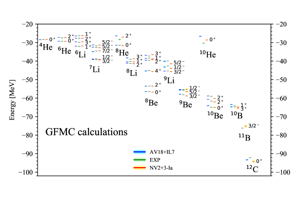
Figure 3: Spectra of $A\,$= 4–12 nuclei. The energy spectra obtained with the NV2+3-Ia chiral interactions are compared to experimental data. Also shown are results obtained with the phenomenological AV18+IL7 interactions.

References

- (1) Carlson, J. et al. Quantum Monte Carlo methods for nuclear physics. Rev. Mod. Phys. 87, 1067 (2015).
- (2) Yukawa, H. On the interactions of elementary particles. Proc. Phys. Math. Soc. Japan 17, 48 (1935).
- (3) Stoks, V.G.J., Klomp, R.A.M., Terheggen, C.P.F. & de Swart, J.J. Construction of high-quality potential models. Phys. Rev. C 49, 2950 (1994).
- (4) Wiringa, R.B., Stoks, V.G.J. & Schiavilla, R. Accurate nucleon-nucleon potential with charge-independence breaking. Phys. Rev. C 51, 38 (1995).
- (5) Machleidt, R. High-precision, charge-dependent Bonn nucleon-nucleon potential. Phys. Rev. C 63, 024001 (2001).
- (6) Stoks, V.G.J., Klomp, R.A.M., Rentmeester, M.C.M. & de Swart, J.J. Partial-wave analysis of all nucleon-nucleon scattering data below 350 MeV. Phys. Rev. C 48, 792 (1993).
- (7) Friar, J.L., Gibson, B.F. & Payne, G.L. Recent Progress in Understanding Trinucleon Properties. Annu. Rev. Nucl. Part. Sci. 34, 403 (1984).
- (8) Pudliner, B.S., Pandharipande, V.R., Carlson, J., Pieper, S.C. & Wiringa, R.B. Quantum Monte Carlo calculations of nuclei with . Phys. Rev. C 56, 1720 (1997).
- (9) Navrátil, P., Vary, J.P. & Barrett, B.R. Large-basis ab initio no-core shell model and its application to 12C. Phys. Rev. C 62, 054311 (2000).
- (10) Pieper, S.C., Pandharipande, V.R., Wiringa, R.B. & Carlson, J. Realistic models of pion-exchange three-nucleon interactions. Phys. Rev. C 64, 014001 (2001).
- (11) Fujita, J. & Miyazawa, H. Pion theory of three-body forces. Prog. Theor. Phys. 17, 360 (1957).
- (12) Pieper, S.C. The Illinois extension to the Fujita-Miyazawa three-nucleon force. AIP Conf. Proc. 1011, 143 (2008).
- (13) Weinberg, S. Nuclear forces from chiral lagrangians. Phys. Lett. B 251, 288 (1990).
- (14) Weinberg, S. Effective chiral lagrangians for nucleon-pion interactions and nuclear forces. Nucl. Phys. B 363, 3 (1991).
- (15) Weinberg, S. Three-body interactions among nucleons and pions. Phys. Lett. B 295, 114 (1992).
- (16) Park, T.-S., Min, D.-P. & Rho, M. Chiral dynamics and heavy-fermion formalism in nuclei: exchange axial currents. Phys. Rep. 233, 341 (1993).
- (17) Park, T.-S., Min, D.-P. & Rho, M. Chiral Lagrangian approach to exchange vector currents in nuclei. Nucl. Phys. A 596, 515 (1996).
- (18) Park, T.-S. et al. Parameter-free effective field theory calculation for the solar proton-fusion and hep processes. Phys. Rev. C 67, 055206 (2003).
- (19) Ordonez, C., Ray, L. & and van Kolck, U. Two-nucleon potential from chiral Lagrangians. Phys. Rev. C 53, 2086 (1996).
- (20) Epelbaum, E., Glöckle, W. & Meissner, U.-G. Nuclear forces from chiral Lagrangians using the method of unitary transformation (I): Formalism. Nucl. Phys. A 637, 107 (1998).
- (21) Entem, D.R. & and Machleidt, R. Accurate charge-dependent nucleon-nucleon potential at fourth order of chiral perturbation theory. Phys. Rev. C 68, 041001 (2003).
- (22) Machleidt, R. & Entem, D.R. Chiral effective field theory and nuclear forces. Phys. Rep. 503, 1 (2011).
- (23) van Kolck, U. Few-nucleon forces from chiral Lagrangians. Phys. Rev. C 49, 2932 (1994).
- (24) Epelbaum, E. et al. Three-nucleon forces from chiral effective field theory Phys. Rev. C 66, 064001 (2002).
- (25) V. Bernard, V., Epelbaum, E., Krebs, H. & Meissner, U.-G. Subleading contributions to the chiral three-nucleon force. II. Short-range terms and relativistic corrections Phys. Rev. C 84, 054001 (2011).
- (26) Girlanda, L., Kievsky, A. & Viviani, M. Subleading contributions to the three-nucleon contact interaction. Phys. Rev. C 84, 014001 (2011).
- (27) Krebs, H., Gasparyan, A. & Epelbaum. Chiral three-nucleon force at N4LO: Longest-range contributions. Phys. Rev. C 85, 054006 (2012).
- (28) Friar, J.L. & van Kolck, U. Charge-independence breaking in the two-pion-exchange nucleon-nucleon force. Phys. Rev. C 60, 034006 (1999).
- (29) Friar, J.L., van Kolck, U., Rentmeester, M.C.M. & Timmermans, R.G.E. Nucleon-mass difference in chiral perturbation theory and nuclear forces Phys. Rev. C 70, 044001 (2004).
- (30) Friar, J.L., Payne, G.L. & van Kolck, U. Charge-symmetry-breaking three-nucleon forces. Phys. Rev. C 71, 024003 (2005).
- (31) Gezerlis, A. et al. Quantum Monte Carlo Calculations with Chiral Effective Field Theory Interactions. Phys. Rev. Lett. 111 (3), 032501 (2013).
- (32) Piarulli, M. et al. Local chiral potentials with -intermediate states and the structure of light nuclei. Phys. Rev. C 94, 054007 (2016).
- (33) Piarulli, M. et al. Minimally nonlocal nucleon-nucleon potentials with chiral two-pion exchange including resonances. Phys. Rev. C 91, 024003 (2015).
- (34) Pérez, R.N., Amaro, J.E. & Arriola, E.R. Partial-wave analysis of nucleon-nucleon scattering below the pion-production threshold. Phys. Rev. C 88, 024002 (2013); ibidem, 069902(E) (2013).
- (35) Lynn, J.E. et al. Chiral Three-Nucleon Interactions in Light Nuclei, Neutron- Scattering, and Neutron Matter. Phys. Rev. Lett. 116, 062501 (2016).
- (36) Lynn, J.E. et al. Quantum Monte Carlo calculations of light nuclei with local chiral two- and three-nucleon interactions. arXiv:1706.07668
- (37) Fettes, N., Meissner, U.-G., Mojzis, M. & Steininger, S. The chiral effective pion-nucleon Lagrangian of order . Ann. Phys. 283, 273 (2000); ibidem 288, 249 (E) (2001).
- (38) Kievsky, A., Rosati, S., Viviani, M., Marcucci, L.E. & Girlanda, L. A high-precision variational approach to three- and four-nucleon bound and zero-energy scattering states. J. Phys. G: Nucl. Part. Phys. 35, 063101 (2008).
- (39) Schoen, K. et al. Precision neutron interferometric measurements and updated evaluations of the n-p and n-d coherent neutron scattering lengths. Phys. Rev. C 67, 044005 (2003).
- (40) Audi, G., Wapstra, A.H. & Thibault, C. The AME2003 atomic mass evaluation (II). Tables, graphs and references. Nucl. Phys. A 729, 337 (2003).
- (41) Shimizu, S. et al.. Analyzing powers of scattering below the deuteron breakup threshold. Phys. Rev. C 52, 1193 (1995).
- (42) Glöckle, W., Witala, H., Hüber, D., Kamada, H. & Golak, J. The three-nucleon continuum: achievements, challenges and applications. Phys. Rep. 274, 107 (1996).
- (43) Golak, J. et al. Low-energy neutron-deuteron reactions with N3LO chiral forces. Eur. Phys. J. A 50, 177 (2014).
- (44) Viviani, M., Kievsky, A. & Rosati, S. Calculation of the -particle ground state within the hyperspherical harmonic basis. Phys. Rev. C 71, 024006 (2005).
- (45) Kievsky, A., Viviani M. & Rosati, S. Polarization observables in - scattering below 30 MeV. Phys. Rev. C 64, 024002 (2001).
- (46) Lusk, E., Butler, R. & Pieper, S.C. Evolution of a minimal parallel programming model. The International Journal of High Performance Computing Applications DOI: 10.1177-1094342017703448 (2017).
- (47) Pastore, S., Wiringa, R.B., Pieper, S.C. & Schiavilla, R. Quantum Monte Carlo calculations of electromagnetic transitions in 8Be with meson-exchange currents derived from chiral effective field theory. Phys. Rev. C 90, 024321 (2014).
- (48) Pastore, S., Pieper, S.C., Schiavilla, R. & Wiringa, R.B. Quantum Monte Carlo calculations of electromagnetic moments and transitions in nuclei with meson-exchange currents derived from chiral effective field theory Phys. Rev. C 86, 024315 (2013).
Acknowledgments
The work of M.P., A.L., E.L., S.C.P., and R.B.W has been supported by the NUclear Computational Low-Energy Initiative (NUCLEI) SciDAC project. This research is further supported by the U.S. Department of Energy, Office of Science, Office of Nuclear Physics, under contracts DE-AC02-06CH11357 (M.P., A.L., S.C.P., and R.B.W.) and DE-AC05-06OR23177 (R.S.). It used computational resources provided by Argonne’s Laboratory Computing Resource Center, by the Argonne Leadership Computing Facility, which is a DOE Office of Science User Facility supported under Contract DE-AC02-06CH11357 (via a Theta Early Science grant), and by the National Energy Research Scientific Computing Center (NERSC).