Exciton-phonon interaction breaking all antiunitary symmetries in external magnetic fields

Abstract

Recent experimental investigations by M. Aßmann et al. [Nature Mater. 15, 741 (2016)] on the spectrum of magnetoexcitons in cuprous oxide revealed the statistics of a Gaussian unitary ensemble (GUE). The model of F. Schweiner et al. [Phys. Rev. Lett. 118, 046401 (2017)], which includes the complete cubic valence band structure of the solid, can explain the appearance of GUE statistics if the magnetic field is not oriented in one of the symmetry planes of the cubic lattice. However, it cannot explain the experimental observation of GUE statistics for all orientations of the field. In this paper we investigate the effect of quasi-particle interactions or especially the exciton-phonon interaction on the level statistics of magnetoexcitons and show that the motional Stark field induced by the exciton-phonon interaction leads to the occurrence of GUE statistics for arbitrary orientations of the magnetic field in agreement with experimental observations. Importantly, the breaking of all antiunitary symmetries can be explained only by considering both the exciton-phonon interaction and the cubic crystal lattice.

I Introduction

Excitons are fundamental quasi-particles in semiconductors, which are the elementary excitations of the electronic system. Consisting of a negatively charged electron in the conduction band and a positively charge hole in the valence band, which interact via a screened Coulomb interaction, excitons are often regarded as the hydrogen analog of the solid state. Especially excitons in cuprous oxide $\left(\mathrm{Cu_{2}O}\right)$ are of interest due to their high Rydberg energy. Only three years ago an almost perfect hydrogen-like absorption series has been observed in $\mathrm{Cu_{2}O}$ up to a principal quantum number of $n=25$ by T. Kazimierczuk et al. Kazimierczuk et al. (2014). This experiment has opened the field of research of giant Rydberg excitons and has stimulated a large number of experimental and theoretical investigations Schweiner et al. (2016a); Grünwald et al. (2016); Feldmaier et al. (2016); Thewes et al. (2015); Schöne et al. (2016); Schweiner et al. (2016b, 2017a); Heckötter et al. (2017); Zielińska-Raczyńska et al. (2017); Schweiner et al. (2016c); Zielińska-Raczyńska et al. (2016a, b); Schweiner et al. (2017b, c), in particular as concerns the level statistics and symmetry-breaking effects Aßmann et al. (2016); Freitag et al. (2017); Schweiner et al. (2017d, e).

If symmetries are broken, the classical dynamics of a system often becomes nonintegrable and chaotic. However, since the description of chaos by trajectories and Lyapunov exponents is not possible in quantum mechanics, classical chaos manifests itself in quantum mechanics in a different way Haake (2010); Stöckmann (1999). The Bohigas-Giannoni-Schmit conjecture Bohigas et al. (1984) suggests that quantum systems with few degrees of freedom and with a chaotic classical limit can be described by random matrix theory Mehta (2004); Porter (1965) and show typical level spacings. If the classical dynamics is regular, the level spacing obeys Poissonian statistics. At the transition to chaos, the level spacing statistics changes to the statistics of a Gaussian orthogonal ensemble (GOE), a Gaussian unitary ensemble (GUE) or a Gaussian symplectic ensemble (GSE) as symmetry reduction leads to a correlation of levels and hence to a strong suppression of crossings Haake (2010). To which of the three universality classes, i.e., to the orthogonal, the unitary or the symplectic universality class, a given system belongs is determined by the remaining symmetries in the system. While GOE statistics appears if there is at least one remaining antiunitary symmetry in the system, for GUE statistics all antiunitary symmetries have to be broken. GSE statistics can be observed for systems with time-reversal invariance possessing Kramer’s degeneracy but no geometric symmetry at all Haake (2010).

The hydrogen-like model of excitons is often too simple to account for the large number of effects due to the surrounding solid. Some essential corrections to this model comprise, e.g., the inclusion of the complete cubic valence band structure Thewes et al. (2015); Schweiner et al. (2016b); Baldereschi and Lipari (1971, 1974, 1973); Lipari and Altarelli (1977); Altarelli and Lipari (1977); Suzuki and Hensel (1974), which leads to a complicated fine-structure splitting, or the interaction with quasi-particles like phonons Schweiner et al. (2016a); Fröhlich (1954); Bardeen and Shockley (1950); Toyozawa (1964).

An important experimental observation by M. Aßmann et al. Aßmann et al. (2016); Freitag et al. (2017), which cannot be explained by the hydrogen-like model, is the appearance of GUE statistics for excitons in an external magnetic field in $\mathrm{Cu_{2}O}$. This observation implies that all antiunitary symmetries are broken in the system. However, for most of the physical systems still there is at least one antiunitary symmetry left Mitchell et al. (2010); Brody et al. (1981); Rosenzweig and Porter (1960); Camarda and Georgopulos (1983); Stöckmann and Stein (1990); Alt et al. (1995, 1996); Zimmermann et al. (1988); Zhou et al. (2010); Vina et al. (1998). This also holds for atoms in constant external fields Held et al. (1998); Frisch et al. (2014); Wintgen and Friedrich (1987). Hence, based on the hydrogen-like model one would expect to observe the statistics of a Gaussian orthogonal ensemble (GOE).

As an explanation, M. Aßmann et al. Aßmann et al. (2016); Freitag et al. (2017) attributed the breaking of all antiunitary symmetries observed for magnetoexcitons to the interaction of excitons with phonons. In a recent letter we have shown theoretically that the combined presence of an external magnetic field and the cubic valence band structure of $\mathrm{Cu_{2}O}$ is sufficient to break all antiunitary symmetries in the system without the need for phonons Schweiner et al. (2017d). However, this breaking appears only if the magnetic field is not oriented in one of the symmetry planes of the cubic lattice of $\mathrm{Cu_{2}O}$. Hence, our model cannot explain the fact that GUE statistics has been observed in the experiment for all directions of the magnetic field Aßmann et al. (2016); Freitag et al. (2017). This raises again the question about the influence of the exciton-phonon interaction on the level spacing statistics of the exciton spectra.

In this paper we will discuss in detail the effects which leads to the appearance of GUE statistics whether or not the external fields are oriented in one of the symmetry planes of the cubic lattice. For fields oriented in a symmetry plane of the laatice, we explain that the interaction of the exciton with other quasi-particles like phonons is not able to restore the broken antiunitary symmetries. As regards the other orientations of the external fields, we discuss that the exciton-phonon interaction leads to a finite momentum of the exciton center of mass and thus to the appearance of a magneto Stark effect in an external magnetic. The electric field connected to this effect then causes in combination with the cubic lattice the breaking of all antiunitary symmetries. Hence, we explain the appearance of GUE statistics for all orientations of the external fields.

The paper is organized as follows: In Sec. II.1 we discuss the Hamiltonian of excitons in $\mathrm{Cu_{2}O}$ when considering the complete valence band structure and the presence of external fields. We explain how to solve the corresponding Schrödinger equation numerically by using a complete basis in Sec. II.2. The calculation of the level spacing distributions is shortly presented in Sec. II.3. We then show the breaking of all antiunitary symmetries in external fields. At first, we treat the case with the plane spanned by the external fields not being identical to one symmetry plane of the lattice in Sec. III. In Sec. IV we discuss the effect of the exciton-phonon interaction and, hence, the motional Stark field, on the spectra if the external fields are oriented in one of the symmetry planes of the lattice. We finally give a short summary and outlook in Sec. V.

II Theory

In this section we briefly introduce the Hamiltonian of excitons in $\mathrm{Cu_{2}O}$ and show how to solve the corresponding Schrödinger equation in a complete basis. Furthermore, we discuss how to determine the level spacing statistics of the exciton spectra numerically and to which level spacing distribution functions the results will be compared. For more details see Refs. Schweiner et al. (2016b, 2017a, 2017e); Schierenberg et al. (2012); Schweiner et al. (2016a) and further references therein.

II.1 Hamiltonian

When neglecting external fields, the Hamiltonian of excitons in direct semiconductors is given by Lipari and Altarelli (1977)

$$H=E_{\mathrm{g}}+V\left(\bm{r}_{e}-\bm{r}_{h}\right)+H_{\mathrm{e}}\left(\bm{p}_{\mathrm{e}}\right)+H_{\mathrm{h}}\left(\bm{p}_{\mathrm{\mathrm{h}}}\right)$$ (1)

with the energy $E_{\mathrm{g}}$ of the band gap between the lowest conduction band and the highest valence band. The Coulomb interaction between the electron (e) and the hole (h) is screened by the dielectric constant $\varepsilon$:

$$V\left(\bm{r}_{e}-\bm{r}_{h}\right)=-\frac{e^{2}}{4\pi\varepsilon_{0}\varepsilon}\frac{1}{\left|\bm{r}_{e}-\bm{r}_{h}\right|}.$$ (2)

Since the conduction band is close to parabolic at zone center, the kinetic energy of the electron is given by the simple expression

$$H_{\mathrm{e}}\left(\bm{p}_{\mathrm{e}}\right)=\frac{\bm{p}_{\mathrm{e}}^{2}}{2m_{\mathrm{e}}},$$ (3)

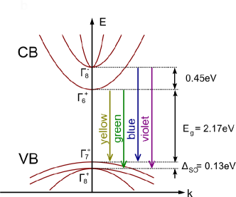
Figure 1: Band structure of $\mathrm{Cu_{2}O}$ Kazimierczuk et al. (2014). As a consequence of the spin-orbit coupling (8) the valence band splits into a lower lying fourfold-degenerate band (including the hole spin) of symmetry $\Gamma_{8}^{+}$ of and a higher lying twofold-degenerate band of symmetry $\Gamma_{7}^{+}$. The lowest lying conduction band of $\mathrm{Cu_{2}O}$ has $\Gamma_{6}^{+}$ symmetry. Depending on the bands involved, one distinguishes between the yellow, green, blue, and violet exciton series. Due to the cubic symmetry of $\mathrm{Cu_{2}O}$, the symmetry of the bands can be assigned by the irreducible representations $\Gamma_{i}^{\pm}$ of the cubic group $O_{\mathrm{h}}$, where the superscript $\pm$ denotes the parity.

with the effective mass $m_{\mathrm{e}}$ of the electron. As regards the valence bands, the situation is more complicated. In all crystals with zinc-blende and diamond structure the valence band is threefold degenerate at the center of the first Brillouin zone or the $\Gamma$ point Lipari and Altarelli (1977); Cohen and Bergstresser (1966). Due to the spin-orbit coupling Rössler (2009); Klingshirn (2007), the degeneracy is lifted in $\mathrm{Cu_{2}O}$ and two of the three valence bands are shifted towards lower energies French et al. (2009). This is shown in Fig. 1. The competition between the dispersion of the threefold degenerate orbital valence band with the spin-orbit splitting is responsible for a strong non-parabolicity of the valence bands.

The kinetic energy of a hole within these valence bands is given by Suzuki and Hensel (1974); Schöne et al. (2016); Schweiner et al. (2016b)

$$H_{\mathrm{h}}\left(\bm{p}_{\mathrm{h}}\right) = H_{\mathrm{so}}+\left(1/2\hbar^{2}m_{0}\right)\left\{\hbar^{2}\left(\gamma_{1}+4\gamma_{2}\right)\bm{p}_{\mathrm{h}}^{2}\right.\phantom{\frac{1}{1}}$$ (4)

$$+ 2\left(\eta_{1}+2\eta_{2}\right)\bm{p}_{\mathrm{h}}^{2}\left(\bm{I}\cdot\bm{S}_{\mathrm{h}}\right)\phantom{\frac{1}{1}}$$

$$- 6\gamma_{2}\left(p_{\mathrm{h}1}^{2}\bm{I}_{1}^{2}+\mathrm{c.p.}\right)-12\eta_{2}\left(p_{\mathrm{h}1}^{2}\bm{I}_{1}\bm{S}_{\mathrm{h}1}+\mathrm{c.p.}\right)\phantom{\frac{1}{1}}$$

$$- 12\gamma_{3}\left(\left\{p_{\mathrm{h}1},p_{\mathrm{h}2}\right\}\left\{\bm{I}_{1},\bm{I}_{2}\right\}+\mathrm{c.p.}\right)\phantom{\frac{1}{1}}$$

$$- \left.12\eta_{3}\left(\left\{p_{\mathrm{h}1},p_{\mathrm{h}2}\right\}\left(\bm{I}_{1}\bm{S}_{\mathrm{h}2}+\bm{I}_{2}\bm{S}_{\mathrm{h}1}\right)+\mathrm{c.p.}\right)\right\}\phantom{\frac{1}{1}}$$

with $\bm{p}=\left(p_{1},\,p_{2},\,p_{3}\right)$, $\left\{a,b\right\}=\frac{1}{2}\left(ab+ba\right)$ and c.p. denoting cyclic permutation. The three Luttinger parameters $\gamma_{i}$ as well as the parameters $\eta_{i}$ describe the behavior and the anisotropic effective mass of the hole in the vicinity of the $\Gamma$ point. Note that the parameters $\eta_{i}$ are often much smaller than the Luttinger parameters and are neglected in the following Baldereschi and Lipari (1971); Schöne et al. (2016); Schweiner et al. (2016b). We have recently shown that the inclusion of quartic and higher-order terms in $p$ in the kinetic energies of the electron and the hole is not necessary due to their negligible size Schweiner et al. (2017b).

The quasispin $I=1$ describes the threefold degenerate valence band and is a convenient abstraction to denote the three orbital Bloch functions $xy$, $yz$, and $zx$ Luttinger (1956). The matrices $\bm{I}_{j}$ and $\bm{S}_{\mathrm{h}j}$ denote the three spin matrices of the quasispin $I$ and the hole spin $S_{\mathrm{h}}=1/2$ while $\bm{I}$ and $\bm{S}_{\mathrm{h}}$ are vectors containing these matrices. Hence, the scalar product of these vectors is given by

$$\bm{I}\cdot\bm{S}_{\mathrm{h}}=\sum_{j=1}^{3}\bm{I}_{j}\bm{S}_{\mathrm{h}j}.$$ (5)

The components of the matrices $\bm{I}_{i}$ read Luttinger (1956); Schweiner et al. (2016b)

$$I_{i,\,jk}=-i\hbar\varepsilon_{ijk}$$ (6)

with the Levi-Civita symbol $\varepsilon_{ijk}$.

We have to note that the matrices $\bm{I}_{i}$ of the quasi-spin $I=1$ given by Eq. (6) are not the standard spin matrices $\bm{S}_{i}$ of spin one Messiah (1969). However, a unitary transformation can be found so that $\bm{U}^{\dagger}\bm{I}_{i}\bm{U}=\bm{S}_{i}$ holds. The corresponding transformation matrix reads

$$\bm{U}=\frac{1}{\sqrt{2}}\left(\begin{array}[]{ccc}-1&0&1\\ -i&0&-i\\ 0&\sqrt{2}&0\end{array}\right).$$ (7)

Since in Ref. Messiah (1969) the behavior of the standard spin matrices under symmetry operations such as time reversal and reflections are given, we will use the standard spin matrices in the following but denote them also by $\bm{I}_{i}$.

The spin-orbit coupling $H_{\mathrm{so}}$ in Eq. (4) is given by Luttinger (1956); Uihlein et al. (1981)

$$H_{\mathrm{so}}=\frac{2}{3}\Delta\left(1+\frac{1}{\hbar^{2}}\bm{I}\cdot\bm{S}_{\mathrm{h}}\right)$$ (8)

with the spin-orbit coupling constant $\Delta$. This coupling can be diagonalized by introducing the effective hole spin $J=I+S_{\mathrm{h}}$. We choose the form of the spin-orbit coupling so that the energy of the valence band with $J=1/2$ remains unchanged while the two valence bands with $J=3/2$ are shifted by an amount of $\Delta$ towards lower energies. Note that we neglect the central-cell corrections treated in Ref. Schweiner et al. (2017b) in the Hamiltonian as they do not affect the exciton states of high energy considered here.

The expression for $H_{\mathrm{h}}\left(\bm{p}_{\mathrm{h}}\right)$ can be written in terms of irreducible tensors (see, e.g., Refs. Edmonds (1960); Baldereschi and Lipari (1973); Schweiner et al. (2016b, 2017a)):

$$H_{\mathrm{h}}\left(\bm{p}_{\mathrm{h}}\right) = H_{\mathrm{so}}+\frac{\gamma_{1}}{2m_{0}}p_{\mathrm{h}}^{2}+\frac{\gamma^{\prime}_{1}}{2\hbar^{2}m_{0}}\left[-\frac{\mu^{\prime}}{3}P_{\mathrm{h}}^{(2)}\cdot I^{(2)}+\frac{\delta^{\prime}}{3}\left(\sum_{k=\pm 4}\left[P_{\mathrm{h}}^{(2)}\times I^{(2)}\right]_{k}^{(4)}+\frac{\sqrt{70}}{5}\left[P_{\mathrm{h}}^{(2)}\times I^{(2)}\right]_{0}^{(4)}\right)\right]$$ (9)

In this case one can clearly distinguish between the terms having spherical symmetry and the terms having cubic symmetry. While the first three terms have spherical symmetry, the last part with the coefficient $\delta^{\prime}$ has cubic symmetry. The coefficients $\mu^{\prime}$ and $\delta^{\prime}$ are given in terms of the three Luttinger parameters as $\mu^{\prime}=\left(6\gamma_{3}+4\gamma_{2}\right)/5\gamma^{\prime}_{1}$ and $\delta^{\prime}=\left(\gamma_{3}-\gamma_{2}\right)/\gamma^{\prime}_{1}$ with $\gamma^{\prime}_{1}=\gamma_{1}+m_{0}/m_{\mathrm{e}}$ Baldereschi and Lipari (1973); Uihlein et al. (1981); Schweiner et al. (2016b).

When applying external fields, the corresponding Hamiltonian is obtained via the minimal substitution. We additionally introduce relative and center of mass coordinates Schmelcher and Cederbaum (1992); Ruder et al. (1994); Schmelcher and Cederbaum (1993). Hence, we replace the coordinates and momenta of electron and hole with

$$\bm{r}_{\mathrm{e}} = \bm{R}+\left(m_{\mathrm{h}}/M\right)\bm{r},$$ (10a)

$$\bm{r}_{\mathrm{h}} = \bm{R}-\left(m_{\mathrm{e}}/M\right)\bm{r},$$ (10b)

$$\bm{p}_{\mathrm{e}} = \left(m_{\mathrm{e}}/M\right)\bm{P}+\bm{p}+e\bm{A}\left(\bm{r}\right),$$ (10c)

$$\bm{p}_{\mathrm{h}} = \left(m_{\mathrm{h}}/M\right)\bm{P}-\bm{p}+e\bm{A}\left(\bm{r}\right),$$ (10d)

where $M=m_{\mathrm{e}}+m_{\mathrm{h}}=m_{\mathrm{e}}+m_{0}/\gamma_{1}$ denotes the yellow exciton mass. Then the Hamiltonian of the exciton reads Altarelli and Lipari (1973, 1974); Chen et al. (1987); Knox (1963); Broeckx (1991); Schmelcher and Cederbaum (1992, 1993)

$$H_{\mathrm{exc}} = E_{\mathrm{g}}+V\left(\bm{r}\right)+e\Phi\left(\bm{r}\right)+H_{B}$$ (11)

$$+ H_{\mathrm{e}}\left(\left(m_{\mathrm{e}}/M\right)\bm{P}+\bm{p}+e\bm{A}\left(\bm{r}\right)\right)$$

$$+ H_{\mathrm{h}}\left(\left(m_{\mathrm{h}}/M\right)\bm{P}-\bm{p}+e\bm{A}\left(\bm{r}\right)\right).$$

We use the vector potential $\bm{A}=\left(\bm{B}\times\bm{r}\right)/2$ of a constant magnetic field $\bm{B}$ and the electrostatic potential $\Phi\left(\bm{r}\right)=-\bm{F}\cdot\bm{r}$ of a constant electric field $\bm{F}$.

Since the Hamiltonian depends only on the relative coordinate $\bm{r}$, the generalized momentum of the center of mass is a good quantum number, i.e., $\left[\bm{P},\,H_{\mathrm{exc}}\right]=\bm{0}$, and one can generally set $\bm{P}=\hbar\bm{K}$ Kanehisa (1983); Ruder et al. (1994); Altarelli and Lipari (1977). When neglecting the exciton-phonon interaction, one can especially assume $\bm{K}\approx\bm{0}$, as the wave vector of photons, by which the excitons are created, is very close to the origin of the Brillouin zone Knox (1963).

The additional term $H_{B}$ in Eq. (11) describes the energy of the spins in the magnetic field Luttinger (1956); Broeckx (1991); Suzuki and Hensel (1974); Altarelli and Lipari (1974):

$$H_{B}=\mu_{\mathrm{B}}\left[g_{c}\bm{S}_{\mathrm{e}}+\left(3\kappa+g_{s}/2\right)\bm{I}-g_{s}\bm{S}_{\mathrm{h}}\right]\cdot\bm{B}/\hbar.$$ (12)

Here $\mu_{B}$ denotes the Bohr magneton, $g_{s}\approx 2$ the $g$-factor of the hole spin $S_{\mathrm{h}}$, $g_{c}$ the $g$-factor of the conduction band or the electron spin $S_{\mathrm{e}}$, and $\kappa$ the fourth Luttinger parameter. All relevant material parameters of $\mathrm{Cu_{2}O}$ are listed in Table 1.

Table 1: Material parameters of $\mathrm{Cu_{2}O}$.

band gap energy	$E_{\mathrm{g}}=2.17208\,\mathrm{eV}$	Kazimierczuk et al. (2014)
electron mass	$m_{\mathrm{e}}=0.99\,m_{0}$	Hodby et al. (1976)
dielectric constant	$\varepsilon=7.5$	Madelung and Rössler (1982-2001)
spin-orbit coupling	$\Delta=0.131\,\mathrm{eV}$	Schöne et al. (2016)
Luttinger parameters	$\gamma_{1}=1.76$	Schöne et al. (2016); Schweiner et al. (2016b)
	$\gamma_{2}=0.7532$	Schöne et al. (2016); Schweiner et al. (2016b)
	$\gamma_{3}=-0.3668$	Schöne et al. (2016); Schweiner et al. (2016b)
	$\kappa=-0.5$	Schweiner et al. (2017a)
$g$-factor of cond. band	$g_{\mathrm{c}}=2.1$	Artyukhin (2012)

As we will show in Sec. III, the symmetry breaking in the system depends on the orientation of the fields with respect to the crystal lattice. We will denote the orientation of $\bm{B}$ and $\bm{F}$ in spherical coordinates via

$$\bm{B}\left(\varphi,\,\vartheta\right)=B\left(\begin{array}[]{c}\cos\varphi\sin\vartheta,\\ \sin\varphi\sin\vartheta\\ \cos\vartheta\end{array}\right)$$ (13)

and similar for $\bm{F}$ in what follows.

Before we solve the Schrödinger equation corresponding to the Hamiltonian (11), we rotate the coordinate system to make the quantization axis coincide with the direction of the magnetic field (see Appendix A) and then express the Hamiltonian (11) in terms of irreducible tensors Edmonds (1960); Baldereschi and Lipari (1973); Broeckx (1991).

II.2 Complete basis

For our numerical investigations, we calculate a matrix representation of the Schrödinger equation corresponding to the Hamiltonian $H_{\mathrm{exc}}$ of Eq. (11) using a complete basis.

As regards the angular momentum part of the basis, we have to consider that the spin orbit coupling $H_{\mathrm{so}}$ couples the quasispin $I$ and the hole spin $S_{\mathrm{h}}$ to the effective hole spin $J=I+S_{\mathrm{h}}$. The remaining parts of the kinetic energy of the hole couple the effective hole spin $J$ and the angular momentum $L$ of the exciton to the effective angular momentum $F=L+J$. The electron spin $S_{\mathrm{e}}$ or its $z$ component $M_{S_{\mathrm{e}}}$ is a good quantum number. For the radial part of the exciton wave function we use the Coulomb-Sturmian functions of Ref. Caprio et al. (2012)

$$U_{NL}\left(r\right)=N_{NL}\left(2\rho\right)^{L}e^{-\rho}L_{N}^{2L+1}\left(2\rho\right)$$ (14)

with $\rho=r/\alpha$, a normalization factor $N_{NL}$, the associated Laguerre polynomials $L_{n}^{m}\left(x\right)$ and an arbitrary scaling parameter $\alpha$. Note that we use the radial quantum number $N$, which is related to the principal quantum number $n$ via $n=N+L+1$. Finally, we make the following ansatz for the exciton wave function

$$\left|\Psi\right\rangle = \sum_{NLJFM_{F}}c_{NLJFM_{F}}\left|\Pi\right\rangle\left|S_{\mathrm{e}},M_{S_{\mathrm{e}}}\right\rangle,$$ (15a)

$$\left|\Pi\right\rangle = \left|N,\,L;\,\left(I,\,S_{\mathrm{h}}\right)\,J;\,F,\,M_{F}\right\rangle$$ (15b)

with complex coefficients $c$. The parenthesis and semicolons in Eq. (15b) shall illustrate the coupling scheme of the spins and the angular momenta.

Inserting the ansatz (15) in the Schrödinger equation $H\Psi=E\Psi$ and multiplying from the left with another basis state $\left\langle\Pi^{\prime}\right|$ yields a matrix representation of the Schrödinger equation of the form Schweiner et al. (2017d)

$$\bm{D}\bm{c}=E\bm{M}\bm{c}.$$ (16)

The vector $\bm{c}$ contains the coefficients of the expansion (15). Since the functions $U_{NL}\left(r\right)$ actually depend on the coordinate $\rho=r/\alpha$, we substitute $r\rightarrow\rho\alpha$ in the Hamiltonian (11) and multiply the corresponding Schrödinger equation by $\alpha^{2}$. All matrix elements which enter the hermitian matrices $\bm{D}$ and $\bm{M}$ can be calculated similarly to the matrix elements given in Refs. Schweiner et al. (2016b, 2017a). The generalized eigenvalue problem (16) is finally solved using an appropriate LAPACK routine Anderson et al. (1999).

Since in numerical calculations the basis cannot be infinitely large, the values of the quantum numbers are chosen in the following way: For each value of $n=N+L+1\leq n_{\mathrm{max}}$ we use

$$L = 0,\,\ldots,\,n-1,$$

$$J = 1/2,\,3/2,$$

$$F = \left|L-J\right|,\,\ldots,\,\min\left(L+J,\,F_{\mathrm{max}}\right),$$ (17)

$$M_{F} = -F,\,\ldots,\,F.$$

The values $F_{\mathrm{max}}$ and $n_{\mathrm{max}}$ are chosen appropriately large so that as many eigenvalues as possible converge. Additionally, we can use the scaling parameter $\alpha$ to enhance convergence Caprio et al. (2012). However, it should be noted that the value of $\alpha$ does not influence the theoretical results for the exciton energies in any way, i.e., the converged results do not depend on the value of $\alpha$.

II.3 Level spacing distributions

Having solved the generalized eigenvalue problem (16) the level statistics of the exciton spectra can be determined. Before analyzing the nearest-neighbor spacings, we have to unfold the spectra to obtain a constant mean spacing Schweiner et al. (2017e); Wintgen and Friedrich (1987); Haake (2010); Bohigas et al. (1984); Brody et al. (1981). The unfolding procedure separates the average behavior of the non-universal spectral density from universal spectral fluctuations and yields a spectrum in which the mean level spacing is equal to unity Schierenberg et al. (2012). We leave out a certain number of low-lying sparse levels to remove individual but nontypical fluctuations Wintgen and Friedrich (1987).

Since the external fields break all symmetries in the system and limit the convergence of the solutions of the generalized eigenvalue problem with high energies Schweiner et al. (2016b), the number of level spacings analyzed here is comparatively small. In this case, the cumulative distribution function Grosa et al. (2014)

$$F(s)=\int_{0}^{s}P(x)\,\mathrm{d}x$$ (18)

is often more meaningful than histograms of the level spacing probability distribution function $P(s)$.

We will compare our results with the distribution functions known from random matrix theory Bohigas et al. (1984); Aßmann et al. (2016): the Poissonian distribution

$$P_{\mathrm{P}}(s)=e^{-s}$$ (19)

for non-interacting energy levels, the Wigner distribution

$$P_{\mathrm{GOE}}(s)=\frac{\pi}{2}\,se^{-\pi s^{2}/4},$$ (20)

and the distribution

$$P_{\mathrm{GUE}}(s)=\frac{32}{\pi^{2}}\,s^{2}e^{-4s^{2}/\pi}$$ (21)

for systems without any antiunitary symmetry. Note that the most characteristic feature of GOE or GUE statistics is the linear or quadratic level repulsion for small $s$, respectively.

In Ref. Schierenberg et al. (2012) also analytical expressions for the spacing distribution functions in the transition region between the different statistics have been derived using random matrix theory for $2\times 2$ matrices. As in our case only the transition from GOE to GUE statistics will be important, we only give the analytical formula for this transition:

$$P_{\mathrm{GOE}\rightarrow\mathrm{GUE}}\left(s;\,\lambda\right)=Cse^{-D^{2}s^{2}}\mathrm{erf}\left(\frac{Ds}{\lambda}\right)$$ (22a)

with

$$D\left(\lambda\right) = \frac{\sqrt{1+\lambda^{2}}}{\sqrt{\pi}}\left(\frac{\lambda}{1+\lambda^{2}}+\mathrm{arccot}\left(\lambda\right)\right),$$ (22b)

$$C\left(\lambda\right) = 2\sqrt{1+\lambda^{2}}D\left(\lambda\right)^{2}.$$ (22c)

For the special cases of $\lambda\rightarrow 0$ or $\lambda\rightarrow\infty$ GOE or GUE statistics is obtained, respectively. However, already for $\lambda\gtrsim 0.8$ the transition to GUE statistics is almost completed Schierenberg et al. (2012).

As in Ref. Schierenberg et al. (2012), we calculate the distribution functions for $\lambda=0.01\times 1000^{(k-1)/999}$ with $k=1,\ldots,1000$ and then numerically integrate the results to obtain the corresponding cumulative distribution functions $F_{\mathrm{GOE}\rightarrow\mathrm{GUE}}\left(s;\,\lambda\right)$.

III Fields not oriented in symmetry plane of the lattice

In a previous paper Schweiner et al. (2017d) we have shown analytically that the last remaining antiunitary symmetry known from the hydrogen atom in external fields is broken for the exciton Hamiltonian (11) if the plane spanned by the external fields is not identical to one of the symmetry planes of the solid. Here we discuss this symmetry breaking in more detail and also explain that the presence of quasi-particle interactions will not restore the broken symmetries.

In the special case of $\gamma_{2}=\gamma_{3}=0$, the exciton Hamiltonian (11) is of the same form as the Hamiltonian of a hydrogen atom in external fields. It is well known that this Hamiltonian is invariant under the combined symmetry of time inversion $K$ followed by a reflection $S_{\hat{\bm{n}}}$ at the specific plane spanned by both fields Haake (2010). This plane is given by the normal vector

$$\hat{\bm{n}}=\left(\bm{B}\times\bm{F}\right)/\left|\bm{B}\times\bm{F}\right|$$ (23)

or $\hat{\bm{n}}\perp\hat{\bm{B}}=\bm{B}/B$ if $\bm{F}=\bm{0}$ holds. Due to this antiunitary symmetry, the hydrogen-like system shows GOE statistics in the chaotic regime Friedrich and Wintgen (1989); Wintgen and Friedrich (1987). However, we have to note that this is the last remaining antiunitary symmetry when applying external fields.

Since the hydrogen atom is spherically symmetric in the field-free case, it makes no difference whether the magnetic field is oriented in $z$ direction or not. However, in a semiconductor with $\delta^{\prime}\neq 0$ the exciton Hamiltonian has cubic symmetry and the orientation of the external fields with respect to the crystal axis of the lattice becomes important. Any rotation of the coordinate system with the aim of making the $z$ axis coincide with the direction of the magnetic field will also rotate the cubic crystal lattice. Hence, the antiunitary symmetry mentioned above is only present if the plane spanned by both fields is identical to one of the nine symmetry planes of the cubic lattice since then the reflection $S_{\hat{\bm{n}}}$ transforms the lattice into itself. However, if none of the normal vectors $\hat{\bm{n}}_{i}$ of these nine symmetry planes (cf. Appendix B) is parallel to the direction $\hat{\bm{n}}$ given in Eq. (23), or, in the case of $\bm{F}=\bm{0}$, if none of these vectors is perpendicular to $\hat{\bm{B}}=\bm{B}/B$, the last antiunitary symmetry is broken. In these cases the commutator of the exciton Hamiltonian (11) with the operator $KS_{\hat{\bm{n}}}$ does not vanish as we will show in the following.

Under time inversion $K$ and reflections $S_{\hat{\bm{n}}}$ at a plane perpendicular to a normal vector $\hat{\bm{n}}$ the vectors of position $\bm{r}$, momentum $\bm{p}$ and spin $\bm{S}$ transform according to Messiah (1969)

$$K\bm{r}K^{\dagger} = \bm{r},$$ (24a)

$$K\bm{p}K^{\dagger} = -\bm{p},$$ (24b)

$$K\bm{S}K^{\dagger} = -\bm{S},$$ (24c)

and

$$S_{\hat{\bm{n}}}\bm{r}S_{\hat{\bm{n}}}^{\dagger} = \bm{r}-2\hat{\bm{n}}\left(\hat{\bm{n}}\cdot\bm{r}\right),$$ (25a)

$$S_{\hat{\bm{n}}}\bm{p}S_{\hat{\bm{n}}}^{\dagger} = \bm{p}-2\hat{\bm{n}}\left(\hat{\bm{n}}\cdot\bm{p}\right),$$ (25b)

$$S_{\hat{\bm{n}}}\bm{S}S_{\hat{\bm{n}}}^{\dagger} = -\bm{S}+2\hat{\bm{n}}\left(\hat{\bm{n}}\cdot\bm{S}\right).$$ (25c)

For all orientations of the external fields the hydrogen-like part of the Hamiltonian (11) is invariant under $KS_{\hat{\bm{n}}}$ with $\hat{\bm{n}}$ given by Eq. (23). However, other parts of the Hamiltonian such as $H_{c}=\left(p_{1}^{2}\bm{I}_{1}^{2}+\mathrm{c.p.}\right)$ are not invariant if the fields are not oriented in one symmetry plane of the lattice. For example, for the case with $\bm{B}\left(0,\,0\right)$ and $\bm{F}\left(\pi/6,\,\pi/2\right)$, we obtain

$$S_{\hat{\bm{n}}}KH_{c}K^{\dagger}S_{\hat{\bm{n}}}^{\dagger}-H_{c}$$ (26)

$$= 1/8\left[2\sqrt{3}\left(\bm{I}_{2}^{2}-\bm{I}_{1}^{2}\right)p_{1}p_{2}\right.$$

$$+ 3\left(\bm{I}_{1}^{2}p_{2}^{2}+\bm{I}_{2}^{2}p_{1}^{2}\right)-3\left(\bm{I}_{1}^{2}p_{1}^{2}+\bm{I}_{2}^{2}p_{2}^{2}\right)$$

$$+ \left.\left\{\bm{I}_{1},\bm{I}_{2}\right\}\left(2\sqrt{3}\left(p_{2}^{2}-p_{1}^{2}\right)+12p_{1}p_{2}\right)\right]\neq 0$$

with $\hat{\bm{n}}=\left(-1/2,\,\sqrt{3}/2,\,0\right)^{\mathrm{T}}$. Note that even though $H_{c}$ does not depend on the external fields, the normal vector $\hat{\bm{n}}$ is determined by these fields via Eq. (23). Otherwise, the hydrogen-like part of the Hamiltonian would not be invariant under $KS_{\hat{\bm{n}}}$.

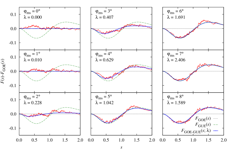
Figure 2: Transition from GOE to GUE statistics when deflecting the field $\bm{F}_{\mathrm{ms}}$ in Eq. (32) from the symmetry plane $y=0$ by an angle $\varphi_{\mathrm{ms}}$. For the magnetic field we have set $\bm{B}\left(\varphi=0,\,\vartheta=\pi/6\right)$ with $B=3\,\mathrm{T}$. To obtain enough eigenvalues for a statistical evaluation, we used the simplified model of Ref. Schweiner et al. (2017d), in which the spins of the electron and hole are neglected. To visualize the differences between the cumulative distribution functions more clearly, we subtract $F_{\mathrm{GOE}}(s)$ from them. The data points (red) were fitted with the analytical function $F_{\mathrm{GOE}\rightarrow\mathrm{GUE}}\left(s;\,\lambda\right)$ defined in Sec. II.3. The optimum values of the fit parameter $\lambda$ are given in each panel and are also shown in Fig. 3. One can observe a good agreement between the numerical data and the analytical function describing the transition between the two statistics in dependence on $\lambda$. For further information see text. 

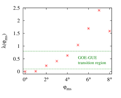
Figure 3: Optimum values of the fit parameter $\lambda$ in dependence on the angle $\varphi_{\mathrm{ms}}$ for the situation presented in Fig. 2. One can see that the value of $\lambda$ increases very rapidly with increasing $\varphi_{\mathrm{ms}}$. Already for $\varphi_{\mathrm{ms}}=5\degree$ the transition to GUE statistics is completed. As regards the value of $\lambda$ for $\varphi_{\mathrm{ms}}=8\degree$, we have to note that the function $F_{\mathrm{GOE}\rightarrow\mathrm{GUE}}\left(s;\,\lambda\right)$ only slightly varies for $\lambda\geq 0.8$ and hence small fluctuations in the numerical results will lead to a strong change in $\lambda$. For the transition between GOE and GUE statistics only the range of $0.1\leq\lambda\leq 0.8$ is of importance (green dahed lines) (cf. Ref. cite225). For $\varphi_{\mathrm{ms}}>8\degree$ it is always $\lambda>0.8$ until $\varphi_{\mathrm{ms}}\approx 176\degree$ [cf. Eq. (33)].

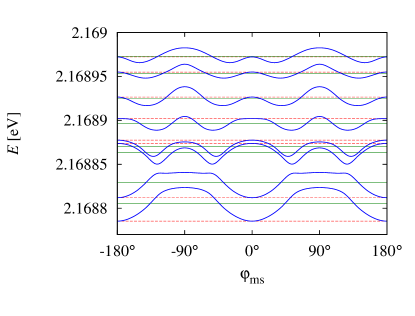
Figure 4: Dependence of the energy of specific exciton states on the angle $\varphi_{\mathrm{ms}}$ of the field $\bm{F}_{\mathrm{ms}}$. For the magnetic field we have set $\bm{B}\left(\varphi=0,\,\vartheta=\pi/6\right)$ with $B=3\,\mathrm{T}$. It can be seen that for $\varphi_{\mathrm{ms}}$ and $\pi+\varphi_{\mathrm{ms}}$ the exciton energies (blue solid lines) are shifted in the same direction with respect to the energy at $\varphi_{\mathrm{ms}}=0$ (red dashed lines). The average energy (green solid lines) often clearly differs from the energy at $\varphi_{\mathrm{ms}}=0$.

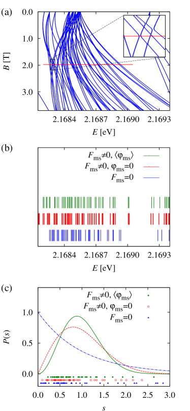
Figure 5: (a) Splitting of the $n=5$ exciton states of $\mathrm{Cu_{2}O}$ in an external magnetic field $\bm{B}=\bm{B}\left(\varphi=0,\,\vartheta=\pi/6\right)$ with $F_{\mathrm{ms}}=0$. At $B\approx 1.98\,\mathrm{T}$ an avoided crossing can be observed (see inset and red box). (b) Energy of the $n=5$ states for $B=1.98\,\mathrm{T}$ and (i) $F_{\mathrm{ms}}=0$ (blue lines), (ii) ${F}_{\mathrm{ms}}=9.57\times 10^{3}\,\mathrm{V/m}$ given by Eq. (32) with $\varphi_{\mathrm{ms}}=0$ (red lines), and (iii) ${F}_{\mathrm{ms}}$ given by Eq. (32) but taking the position of the states when averaging over $\varphi_{\mathrm{ms}}=0$ (green lines). (c) Normalized spacings for the three cases considered. It can be seen that the motional Stark effect further suppresses small spacings. For a comparison, we also show the distribution functions for Poisson statistics (blue dash-dotted line), GOE statistics (red dashed line), and GUE statistics (green solid line).

Since the expression in Eq. (26) is not equal to zero, we have shown for $\bm{B}\left(0,\,0\right)$ and $\bm{F}\left(\pi/6,\,\pi/2\right)$ that the generalized time-reversal symmetry of the hydrogen atom is broken for excitons due to the cubic symmetry of the semiconductor. The same calculation can also be performed for other orientations of the external fields. As we have stated above, the antiunitary symmetry remains unbroken only for those specific orientations of the fields, where $\hat{\bm{n}}$ given by Eq. (23) is parallel to one of the normal vectors in Eq. (39).

In the previous treatment we have neglected quasi-particle interactions like the exciton-phonon interaction. Hence, one may ask whether these interactions are able to restore the broken symmetries.

It is well known that when adding an additional interaction to a Hamiltonian, this interaction will often further reduce the symmetry of the problem and not increase it. Indeed, it is not possible that the effects of the band structure and quasi-particle interactions on the symmetry or the level spacing statistics will cancel each other out, in particular for all values of the external field strengths. The quasi-particle interaction would have to have the same form as the operators in our Hamiltonian to make the commutator of the Hamiltonian and the symmetry operator $KS_{\hat{\bm{n}}}$ vanish. However, if we, e.g., consider the interaction between excitons and phonons, the interaction operators Rössler (2009) look quite different than the operators in the exciton Hamiltonian (11). Hence, phonons or other interactions in the solid do not restore the broken antiunitary symmetries if the external fields are not oriented in one symmetry plane of the solid.

IV Fields oriented in symmetry plane of the lattice

In this section we discuss the case that the plane spanned by the external fields coincides with a symmetry plane of the lattice. Without the exciton-phonon interaction one would expect to observe only GOE statistics according to the explanations given in Sec. III. However, recent experiments indicate that the spectrum of magnetoexcitons reveals GUE statistics for all orientations of the magnetic field applied Aßmann et al. (2016); Freitag et al. (2017). Hence, we will now concentrate on the effects of the exciton-phonon interaction in more detail and show that they lead, in combination with the cubic valence band structure, to a breaking of all antiunitary symmetries for an arbitrary orientation of the external fields.

The Hamiltonian describing the exciton-phonon interaction Rössler (2009) does not only depend on the relative coordinate $\bm{r}$ but also on the coordinate of the center of mass $\bm{R}$. Hence, when considering the Hamiltonian of excitons and photons the momentum of the center of mass $\bm{P}$ is not a good quantum number, i.e., the Hamiltonian and the operator $\bm{P}$ no longer commute. Consequently, we are not allowed to set the momentum of the center of mass to zero, as has been done in the calculation of Sec. III, but have to treat the complete problem. However, the consideration of the valence band structure, a finite momentum of the center of mass, the external fields, and the phonons is very complicated. Hence, we concentrate only on the main effects to show that the exciton-phonon interaction will lead to a breaking of all antiunitary symmetries even if the plane spanned by the external fields is identical to a symmetry plane of the lattice.

When considering a finite momentum $\bm{P}=\hbar\bm{K}$ of the exciton center of mass in an external magnetic field, the motional Stark effect occurs Ruder et al. (1994). Since the insertion of a finite momentum of the center of mass in the complete Hamiltonian (11) is quite laborious (cf. Ref. Schweiner et al. (2017c)), we treat only the leading term of the motional Stark effect, which has the form Ruder et al. (1994)

$$H_{\mathrm{ms}}=\frac{\hbar e}{M}\left(\bm{K}\times\bm{B}\right)\cdot\bm{r}$$ (27)

with the isotropic exciton mass $M=m_{\mathrm{e}}+m_{\mathrm{h}}=m_{\mathrm{e}}+m_{0}/\gamma_{1}$. Note that this term has the same form as the electric field term in the Hamiltonian (11). Hence, the effect of the motional Stark effect is the same as that of an external electric field and we can introduce a total electric field

$$\bm{F}_{\mathrm{tot}}=\bm{F}+\bm{F}_{\mathrm{ms}}=\bm{F}-\frac{\hbar}{M}\left(\bm{K}\times\bm{B}\right).$$ (28)

One could now, in principle, do the same calculation as in Eq. (26) to show that the antiunitary symmetry known from the hydrogen atom is broken if the plane spanned by $\bm{B}$ and $\bm{F}_{\mathrm{tot}}$ is not identical to one symmetry plane of the solid. However, we have to consider the specific properties, i.e., the size and the orientation, of the motional stark field $\bm{F}_{\mathrm{ms}}$ related to the size and the orientation of $\bm{K}$.

The size of the momentum $\hbar\bm{K}$ is determined by the interaction between excitons and phonons. Instead of considering the huge number of phonon degrees of freedom, we assume a thermal distribution at a finite temperature $T$. The direction of $\bm{K}$ is then evenly distributed over the solid angle and its average size is determined by

$$\frac{3}{2}k_{\mathrm{B}}T=\frac{\hbar^{2}K^{2}}{2M}$$ (29)

with the Boltzmann constant $k_{\mathrm{B}}$. We assume for all of our calculations a temperature of $T=0.8\,\mathrm{K}$, which is even slightly smaller than the temperature in experiments Kazimierczuk et al. (2014). The relation (29) leads to a field strength of

$$F_{\mathrm{ms}}=\sqrt{\frac{3k_{\mathrm{B}}T}{M}}\,B.$$ (30)

Note that the value of $K$ determined by Eq. (29) is of the same order of magnitude as the value estimated via experimental group velocity measurements of the $1S$ ortho exciton Fröhlich et al. (2006, 2005).

We will now show that the motional Stark field $\bm{F}_{\mathrm{ms}}$ leads to GUE statistics if the external magnetic field $\bm{B}$ is oriented in one of the symmetry planes of the lattice In the general case, the magnetic field then fulfils $\bm{B}\perp\hat{\bm{n}}_{i}$ with one of the nine normal vectors $\hat{\bm{n}}_{i}$ given in Eq. (39). In our numerical example we choose the magnetic field

$$\bm{B}=\bm{B}\left(\varphi=0,\,\vartheta=\pi/6\right)=\frac{B}{2}\left(\begin{array}[]{c}1\\ 0\\ \sqrt{3}\end{array}\right)\perp\hat{\bm{n}}_{2}$$ (31)

with a constant field strength of $B=3\,\mathrm{T}$. The external electric field is set to $\bm{F}=\bm{0}$. The motional Stark field is oriented perpendicular to $\bm{B}$. Hence, we assume it for $\varphi_{\mathrm{ms}}$ to be oriented perpendicular to the magnetic field and to be initially lying in the same symmetry plane $y=0$ of the lattice. Then $\bm{F}_{\mathrm{ms}}$ is deflected from this plane, i.e., the field is rotated by an angle $\varphi_{\mathrm{ms}}$ about the axis given by the magnetic field of Eq. (31):

$$\bm{F}_{\mathrm{ms}}\left(\varphi_{\mathrm{ms}}\right)=\frac{F_{\mathrm{ms}}}{2}\left(\begin{array}[]{c}\sqrt{3}\cos\varphi_{\mathrm{ms}}\\ 2\sin\varphi_{\mathrm{ms}}\\ -\cos\varphi_{\mathrm{ms}}\end{array}\right).$$ (32)

Here $F_{\mathrm{ms}}$ is given by Eq. (30) with $B=3\,\mathrm{T}$ and $T=1.2\,\mathrm{K}$. According to the explanations given in Sec. III, we expect to obtain GOE statistics with our numerical results only for the cases $\varphi_{\mathrm{ms}}=0$ and $\varphi_{\mathrm{ms}}=\pi$, since

$$\hat{\bm{n}}=\left(\bm{B}\times\bm{F}\right)/\left|\bm{B}\times\bm{F}\right|=\frac{1}{2}\left(\begin{array}[]{c}-\sqrt{3}\sin\varphi_{\mathrm{ms}}\\ 2\cos\varphi_{\mathrm{ms}}\\ \sin\varphi_{\mathrm{ms}}\end{array}\right)$$ (33)

is parallel to $\hat{\bm{n}}_{2}$ only for these two values of $\varphi_{\mathrm{ms}}$. The decisive question is how fast the transition from GOE to GUE statistics takes place if the field $\bm{F}_{\mathrm{ms}}$ is deflected from the symmetry plane $y=0$. This is shown in Fig. 2.

As we have already stated in Ref. Schweiner et al. (2017d) and Sec. II.3, the number of eigenvalues which can be used for a statistical analysis is limited due to the required computer memory or the limited size of our basis. Therefore, to enhance the number of converged states, we used for the calculation of Fig. 2 the simplified model of Ref. Schweiner et al. (2017d) with $\Delta=H_{B}=0$, $m_{\mathrm{e}}=m_{0}$, $\gamma_{1}=2$ and $\delta^{\prime}=-0.15$. However, we expect a qualitatively similar behavior for $\mathrm{Cu_{2}O}$, i.e., when considering $\Delta\neq 0$, as we will discuss and show below.

For a quantitative analysis the results are fitted with the function $F_{\mathrm{GOE}\rightarrow\mathrm{GUE}}\left(s;\,\lambda\right)$ [cf. Eq. (22)] describing the transition between both statistics. We show the resulting values of the fit parameter $\lambda$ in Fig. 3. It can be seen that the parameter $\lambda$ increases very rapidly with increasing values of $\varphi_{\mathrm{ms}}$. Already for $\varphi_{\mathrm{ms}}=5\degree$ the statistics is almost purely GUE statistics. Hence, the motional Stark field has a strong influence on the level spacing statistics. This implies that for a majority of the orientations of $\bm{F}_{\mathrm{ms}}$ GUE statistics will be observable. Our main argument for the observed level statistics is now that since the momentum $\bm{K}$ and hence also the field $\bm{F}_{\mathrm{ms}}$ is evenly distributed over the angle $\varphi_{\mathrm{ms}}$, the exciton spectrum will show GUE statistics on average.

One might argue whether the effects of $\bm{F}_{\mathrm{ms}}$ cancel each other out if the field is evenly distributed over the solid angle. This can be ruled out when considering the effect of the field on the exciton states for all values of the angle $\varphi_{\mathrm{ms}}$ as shown for a selection of exciton states in Fig. 4. It can be seen that the fields $\bm{F}_{\mathrm{ms}}\left(\varphi_{\mathrm{ms}}\right)$ and $\bm{F}_{\mathrm{ms}}\left(\pi+\varphi_{\mathrm{ms}}\right)=-\bm{F}_{\mathrm{ms}}\left(\varphi_{\mathrm{ms}}\right)$ shift the exciton states in the same direction and not in opposite direction as regards their energies. Hence, on average the exciton states are shifted towards higher or lower energies and do not remain at their position. This argument holds both when using the model with the parameters of Ref. Schweiner et al. (2017d) and when using all material parameters of $\mathrm{Cu_{2}O}$. In Fig. 4 the results for $\mathrm{Cu_{2}O}$ are shown.

Even though we cannot obtain enough converged exciton energies for a statistical analysis when using the parameters of $\mathrm{Cu_{2}O}$, we can use the small number of converged states to show that the magneto Stark field has the small effect of increasing level spacings, which is a characteristic feature of GUE compared to GOE statistics [cf. Eqs. (20) and (21)].

To this aim, we consider at first the spectrum of $\mathrm{Cu_{2}O}$ in a magnetic field $\bm{B}\left(\varphi=0,\,\vartheta=\pi/6\right)$ to find an avoided crossing (see panel (a) of Fig. 5). We then choose the magnetic field strength of $B=1.98\,\mathrm{T}$, where an avoided crossing appears, to be fixed, and calculate the spectrum in dependence on the angle $\varphi_{\mathrm{ms}}$. The strength of the motional Stark field is given by Eq. (30) with $B=1.98\,\mathrm{T}$ and $T=1.2\,\mathrm{K}$. We now calculate the energies of the states for the following three cases, where the magnetic field strength is always given by $B=1.98\,\mathrm{T}$: (i) $F_{\mathrm{ms}}=0$, (ii) $F_{\mathrm{ms}}=\sqrt{2k_{\mathrm{B}}T/M}\,B$ and $\varphi_{\mathrm{ms}}=0$, (iii) $F_{\mathrm{ms}}=\sqrt{2k_{\mathrm{B}}T/M}\,B$ and taking the average of the exciton energies over $\varphi_{\mathrm{ms}}$. These energies are shown in panel (b) of Fig. 5. We assume a constant density of states due to the small energy range considered here. Then the normalized spacings between two neighboring exciton states are determined as $s_{i}=(E_{i}-E_{i+1})/\bar{E}$ with $\bar{E}$ denoting the mean value of all spacings considered. One can see from panel (c) of Fig. 5 that the level spacings change for the three cases considered. Especially for small values of $s$ the spacing increases, which illustrates the repulsion of levels and the transition to GUE statistics.

Overall, it can be stated that the exciton-phonon interaction leads to a finite momentum of the center of mass of the exciton, which is evenly distributed over the solid angle. The size of this momentum is on average determined by the Boltzmann distribution. In an external magnetic field this finite momentum causes the motional Stark effect. The electric field corresponding to this effect breaks in combination with the cubic lattice all antiunitary symmetries in the system even if the plane spanned by the external fields coincides with one symmetry plane of the lattice.

V Summary and outlook

We have shown analytically that the combined presence of the cubic valence band structure and external fields breaks all antiunitary symmetries for excitons in $\mathrm{Cu_{2}O}$. When neglecting the exciton-phonon interaction, this symmetry breaking appears only if the plane spanned by the external fields is not identical to one of the symmetry planes of the cubic lattice of $\mathrm{Cu_{2}O}$. We have discussed that for these cases the additional presence of the exciton-phonon interaction is not able to restore the broken symmetries.

For the specific orientations of the external fields, where the plane spanned by the fields is identical to one of the symmetry planes of the cubic lattice, the exciton-phonon interaction becomes important. This interaction causes a finite momentum of the exciton center of mass, which leads to the motional Stark effect in an external magnetic field. If the cubic valence band structure is considered, the effective electric field connected with the motional Stark effect finally leads to the breaking of all antiunitary symmetries. Since the exciton-phonon interaction is always present in the solid, we have thus shown that GUE statistics will be observable in all spectra of magnetoexcitons irrespective of the orientation of the external magnetic field, which is in agreement with the experimental observations in Refs. Aßmann et al. (2016); Freitag et al. (2017).

Appendix A Hamiltonian

Here we give the complete Hamiltonian of Eq. (11) and describe the rotation necessary to make the quantization axis coincide with the direction of the magnetic field. Let us write the Hamiltonian (11) in the form

$$H = H_{0}+(eB)H_{1}+(eB)^{2}H_{2}-e\bm{F}\cdot\bm{r}$$ (34)

$$+ E_{\mathrm{g}}-\frac{e^{2}}{4\pi\varepsilon_{0}\varepsilon}\frac{1}{r}+\frac{2}{3}\Delta\left(1+\frac{1}{\hbar^{2}}\bm{I}\cdot\bm{S}_{\mathrm{h}}\right)$$

with $B=\left|\bm{B}\right|$. Using $\hat{B}_{i}=B_{i}/B$ with the components $B_{i}$ of $\bm{B}$, the terms $H_{0}$, $H_{1}$, and $H_{2}$ are given by

$$H_{0} =\>\frac{1}{2m_{0}}\left(\gamma_{1}^{\prime}+4\gamma_{2}\right)\bm{p}^{2}+\frac{1}{\hbar^{2}m_{0}}\left(\eta_{1}+2\eta_{2}\right)\left(\bm{I}\cdot\bm{S}_{\mathrm{h}}\right)\bm{p}^{2}$$

$$-\frac{3\gamma_{2}}{\hbar^{2}m_{0}}\left[\bm{I}_{1}^{2}p_{1}^{2}+\mathrm{c.p.}\right]-\frac{6\eta_{2}}{\hbar^{2}m_{0}}\left[\bm{I}_{1}\bm{S}_{\mathrm{h}1}p_{1}^{2}+\mathrm{c.p.}\right]$$

$$-\frac{6\gamma_{3}}{\hbar^{2}m_{0}}\left[\left\{\bm{I}_{1},\,\bm{I}_{2}\right\}p_{1}p_{2}+\mathrm{c.p.}\right]-\frac{6\eta_{3}}{\hbar^{2}m_{0}}\left[\left(\bm{I}_{1}\bm{S}_{\mathrm{h}2}+\bm{I}_{2}\bm{S}_{\mathrm{h}1}\right)p_{1}p_{2}+\mathrm{c.p.}\right],$$ (35)

$$H_{1} =\>\frac{1}{2m_{0}}\left(\frac{2m_{0}}{m_{\mathrm{e}}}-\gamma_{1}^{\prime}+4\gamma_{2}\right)\hat{\bm{B}}\cdot\bm{L}-\frac{1}{\hbar^{2}m_{0}}\left(\eta_{1}+2\eta_{2}\right)\left(\bm{I}\cdot\bm{S}_{\mathrm{h}}\right)\hat{\bm{B}}\cdot\bm{L}$$

$$+\frac{1}{2m_{0}}\left[g_{c}\bm{S}_{\mathrm{e}}+\left(3\kappa+\frac{g_{s}}{2}\right)\bm{I}-g_{s}\bm{S}_{\mathrm{h}}\right]\cdot\hat{\bm{B}}$$

$$+\frac{3\gamma_{2}}{\hbar^{2}m_{0}}\left[\bm{I}_{1}^{2}\left(\hat{B}_{2}r_{3}p_{1}-\hat{B}_{3}r_{2}p_{1}\right)+\mathrm{c.p.}\right]+\frac{6\eta_{2}}{\hbar^{2}m_{0}}\left[\bm{I}_{1}\bm{S}_{\mathrm{h}1}\left(\hat{B}_{2}r_{3}p_{1}-\hat{B}_{3}r_{2}p_{1}\right)+\mathrm{c.p.}\right]$$

$$+\frac{3\gamma_{3}}{\hbar^{2}m_{0}}\left[\left\{\bm{I}_{1},\,\bm{I}_{2}\right\}\left(\hat{B}_{2}r_{3}p_{2}-\hat{B}_{1}r_{3}p_{1}+\hat{B}_{3}r_{1}p_{1}-\hat{B}_{3}r_{2}p_{2}\right)+\mathrm{c.p.}\right]$$

$$+\frac{3\eta_{3}}{\hbar^{2}m_{0}}\left[\left(\bm{I}_{1}\bm{S}_{\mathrm{h}2}+\bm{I}_{2}\bm{S}_{\mathrm{h}1}\right)\left(\hat{B}_{2}r_{3}p_{2}-\hat{B}_{1}r_{3}p_{1}+\hat{B}_{3}r_{1}p_{1}-\hat{B}_{3}r_{2}p_{2}\right)+\mathrm{c.p.}\right],$$ (36)

$$H_{2} =\>\frac{1}{8m_{0}}\left(\gamma_{1}^{\prime}+4\gamma_{2}\right)\left[\hat{\bm{B}}^{2}\bm{r}^{2}-\left(\hat{\bm{B}}\cdot\bm{r}\right)^{2}\right]+\frac{1}{4\hbar^{2}m_{0}}\left(\eta_{1}+2\eta_{2}\right)\left(\bm{I}\cdot\bm{S}_{\mathrm{h}}\right)\left[\hat{\bm{B}}^{2}\bm{r}^{2}-\left(\hat{\bm{B}}\cdot\bm{r}\right)^{2}\right]$$

$$-\frac{3\gamma_{2}}{4\hbar^{2}m_{0}}\left[\bm{I}_{1}^{2}\left(\hat{B}_{2}r_{3}-\hat{B}_{3}r_{2}\right)^{2}+\mathrm{c.p.}\right]-\frac{3\eta_{2}}{2\hbar^{2}m_{0}}\left[\bm{I}_{1}\bm{S}_{\mathrm{h}1}\left(\hat{B}_{2}r_{3}-\hat{B}_{3}r_{2}\right)^{2}+\mathrm{c.p.}\right]$$

$$-\frac{3\gamma_{3}}{2\hbar^{2}m_{0}}\left[\left\{\bm{I}_{1},\,\bm{I}_{2}\right\}\left(\hat{B}_{2}r_{3}-\hat{B}_{3}r_{2}\right)\left(\hat{B}_{3}r_{1}-\hat{B}_{1}r_{3}\right)+\mathrm{c.p.}\right]$$

$$-\frac{3\eta_{3}}{2\hbar^{2}m_{0}}\left[\left(\bm{I}_{1}\bm{S}_{\mathrm{h}2}+\bm{I}_{2}\bm{S}_{\mathrm{h}1}\right)\left(\hat{B}_{2}r_{3}-\hat{B}_{3}r_{2}\right)\left(\hat{B}_{3}r_{1}-\hat{B}_{1}r_{3}\right)+\mathrm{c.p.}\right].$$ (37)

In our calculations, we express the magnetic field in spherical coordinates [see Eq. (13)]. For the different orientations of the magnetic field we rotate the coordinate system by

$$\bm{R}=\left(\begin{array}[]{ccc}\cos\varphi\cos\vartheta&\sin\varphi\cos\vartheta&-\sin\vartheta\\ -\sin\varphi&\cos\varphi&0\\ \cos\varphi\sin\vartheta&\sin\varphi\sin\vartheta&\cos\vartheta\end{array}\right),$$ (38)

i.e., we replace $\bm{x}\rightarrow\bm{x}^{\prime}=\bm{R}^{\mathrm{T}}\bm{x}$ with $\bm{x}\in\left\{\bm{r},\,\bm{p},\,\bm{L},\,\bm{I},\,\bm{S}\right\}$ to make the quantization axis coincide with the direction of the magnetic field Broeckx (1991); Edmonds (1960). Finally we express the Hamiltonian in terms of irreducible tensors (see, e.g., Refs. Edmonds (1960); Baldereschi and Lipari (1973); Schweiner et al. (2016b, 2017a)) and calculate the matrix elements of the matrices $\bm{D}$ and $\bm{M}$ in the generalized eigenvalue problem (16).

Appendix B Normal vectors

Here we list the normal vectors the nine symmetry planes of the cubic lattice mentioned in the discussion of Sec. III:

$$\hat{\bm{n}}_{1} = \left(1,\,0,\,0\right)^{\mathrm{T}},$$

$$\hat{\bm{n}}_{2} = \left(0,\,1,\,0\right)^{\mathrm{T}},$$

$$\hat{\bm{n}}_{3} = \left(0,\,0,\,1\right)^{\mathrm{T}},$$

$$\hat{\bm{n}}_{4} = \left(1,\,1,\,0\right)^{\mathrm{T}}/\sqrt{2},$$

$$\hat{\bm{n}}_{5} = \left(0,\,1,\,1\right)^{\mathrm{T}}/\sqrt{2},$$

$$\hat{\bm{n}}_{6} = \left(1,\,0,\,1\right)^{\mathrm{T}}/\sqrt{2},$$

$$\hat{\bm{n}}_{7} = \left(1,\,-1,\,0\right)^{\mathrm{T}}/\sqrt{2},$$

$$\hat{\bm{n}}_{8} = \left(0,\,1,\,-1\right)^{\mathrm{T}}/\sqrt{2},$$

$$\hat{\bm{n}}_{9} = \left(-1,\,0,\,1\right)^{\mathrm{T}}/\sqrt{2}.$$ (39)

References

- Kazimierczuk et al. (2014) T. Kazimierczuk, D. Fröhlich, S. Scheel, H. Stolz, and M. Bayer, Nature 514, 343 (2014).
- Schweiner et al. (2016a) F. Schweiner, J. Main, and G. Wunner, Phys. Rev. B 93, 085203 (2016a).
- Grünwald et al. (2016) P. Grünwald, M. Aßmann, J. Heckötter, D. Fröhlich, M. Bayer, H. Stolz, and S. Scheel, Phys. Rev. Lett. 117, 133003 (2016).
- Feldmaier et al. (2016) M. Feldmaier, J. Main, F. Schweiner, H. Cartarius, and G. Wunner, J. Phys. B: At. Mol. Opt. Phys. 49, 144002 (2016).
- Thewes et al. (2015) J. Thewes, J. Heckötter, T. Kazimierczuk, M. Aßmann, D. Fröhlich, M. Bayer, M. A. Semina, and M. M. Glazov, Phys. Rev. Lett. 115, 027402 (2015), and Supplementary Material.
- Schöne et al. (2016) F. Schöne, S. O. Krüger, P. Grünwald, H. Stolz, S. Scheel, M. Aßmann, J. Heckötter, J. Thewes, D. Fröhlich, and M. Bayer, Phys. Rev. B 93, 075203 (2016).
- Schweiner et al. (2016b) F. Schweiner, J. Main, M. Feldmaier, G. Wunner, and Ch. Uihlein, Phys. Rev. B 93, 195203 (2016b).
- Schweiner et al. (2017a) F. Schweiner, J. Main, G. Wunner, M. Freitag, J. Heckötter, Ch. Uihlein, M. Aßmann, D. Fröhlich, and M. Bayer, Phys. Rev. B 95, 035202 (2017a).
- Heckötter et al. (2017) J. Heckötter, M. Freitag, D. Fröhlich, M. Aßmann, M. Bayer, M. A. Semina, and M. M. Glazov, Phys. Rev. B 95, 035210 (2017).
- Zielińska-Raczyńska et al. (2017) S. Zielińska-Raczyńska, D. Ziemkiewicz, and G. Czajkowski, Phys. Rev. B 95, 075204 (2017).
- Schweiner et al. (2016c) F. Schweiner, J. Main, G. Wunner, and Ch. Uihlein, Phys. Rev. B 94, 115201 (2016c).
- Zielińska-Raczyńska et al. (2016a) S. Zielińska-Raczyńska, G. Czajkowski, and D. Ziemkiewicz, Phys. Rev. B 93, 075206 (2016a).
- Zielińska-Raczyńska et al. (2016b) S. Zielińska-Raczyńska, D. Ziemkiewicz, and G. Czajkowski, Phys. Rev. B 94, 045205 (2016b).
- Schweiner et al. (2017b) F. Schweiner, J. Main, G. Wunner, and Ch. Uihlein, Phys. Rev. B 95, 195201 (2017b).
- Schweiner et al. (2017c) F. Schweiner, J. Main, G. Wunner, and Ch. Uihlein, Phys. Rev. B (2017c), submitted.
- Aßmann et al. (2016) M. Aßmann, J. Thewes, D. Fröhlich, and M. Bayer, Nature Mater. 15, 741 (2016).
- Freitag et al. (2017) M. Freitag, J. Heckötter, M. Bayer, and M. Aßmann, Phys. Rev. B 95, 155204 (2017).
- Schweiner et al. (2017d) F. Schweiner, J. Main, and G. Wunner, Phys. Rev. Lett. 118, 046401 (2017d).
- Schweiner et al. (2017e) F. Schweiner, J. Main, and G. Wunner, Phys. Rev. E 95, 062205 (2017e).
- Haake (2010) F. Haake, Quantum Signatures of Chaos, Springer Series in Synergetics (Springer, Heidelberg, 2010), 3rd ed.
- Stöckmann (1999) H.-J. Stöckmann, Quantum Chaos: An Introduction (Cambridge University Press, Cambridge, 1999).
- Bohigas et al. (1984) O. Bohigas, M. J. Giannoni, and C. Schmit, Phys. Rev. Lett. 52, 1 (1984).
- Mehta (2004) M. L. Mehta, Random Matrices (Elsevier, Amsterdam, 2004), 3rd ed.
- Porter (1965) C. E. Porter, ed., Statistical Theory of Spectra (Academic Press, New York, 1965).
- Baldereschi and Lipari (1971) A. Baldereschi and N. O. Lipari, Phys. Rev. B 3, 439 (1971).
- Baldereschi and Lipari (1974) A. Baldereschi and N. O. Lipari, Phys. Rev. B 9, 1525 (1974).
- Baldereschi and Lipari (1973) A. Baldereschi and N. O. Lipari, Phys. Rev. B 8, 2697 (1973).
- Lipari and Altarelli (1977) N. O. Lipari and M. Altarelli, Phys. Rev. B 15, 4883 (1977).
- Altarelli and Lipari (1977) M. Altarelli and N. O. Lipari, Phys. Rev. B 15, 4898 (1977).
- Suzuki and Hensel (1974) K. Suzuki and J. C. Hensel, Phys. Rev. B 9, 4184 (1974).
- Fröhlich (1954) H. Fröhlich, Advances in Physics 3, 325 (1954).
- Bardeen and Shockley (1950) J. Bardeen and W. Shockley, Phys. Rev. 80, 72 (1950).
- Toyozawa (1964) Y. Toyozawa, J. Phys. Chem. Solids 25, 59 (1964).
- Mitchell et al. (2010) G. E. Mitchell, A. Richter, and H. A. Weidenmüller, Rev. Mod. Phys. 82, 2845 (2010).
- Brody et al. (1981) T. A. Brody, J. Flores, J. B. French, P. A. Mello, A. Pandey, and S. S. M. Wong, Rev. Mod. Phys. 53, 385 (1981).
- Rosenzweig and Porter (1960) N. Rosenzweig and C. E. Porter, Phys. Rev. 120, 1698 (1960).
- Camarda and Georgopulos (1983) H. S. Camarda and P. D. Georgopulos, Phys. Rev. Lett. 50, 492 (1983).
- Stöckmann and Stein (1990) H.-J. Stöckmann and J. Stein, Phys. Rev. Lett. 64, 2215 (1990).
- Alt et al. (1995) H. Alt, H.-D. Gräf, H. L. Harney, R. Hofferbert, H. Lengeler, A. Richter, P. Schardt, and H. A. Weidenmüller, Phys. Rev. Lett. 74, 62 (1995).
- Alt et al. (1996) H. Alt, H.-D. Gräf, R. Hofferbert, C. Rangacharyulu, H. Rehfeld, A. Richter, P. Schardt, and A. Wirzba, Phys. Rev. E 54, 2303 (1996).
- Zimmermann et al. (1988) T. Zimmermann, H. Köppel, L. S. Cederbaum, G. Persch, and W. Demtröder, Phys. Rev. Lett. 61, 3 (1988).
- Zhou et al. (2010) W. Zhou, Z. Chen, B. Zhang, C. H. Yu, W. Lu, and S. C. Shen, Phys. Rev. Lett. 105, 024101 (2010).
- Vina et al. (1998) L. Vina, M. Potemski, and W. Wang, Phys.-Usp. 41, 153 (1998).
- Held et al. (1998) H. Held, J. Schlichter, G. Raithel, and H. Walther, Europhys. Lett. 43, 392 (1998).
- Frisch et al. (2014) A. Frisch, M. Mark, K. Aikawa, F. Ferlaino, J. L. Bohn, C. Makrides, A. Petrov, and S. Kotochigova, Nature 507, 475 (2014).
- Wintgen and Friedrich (1987) D. Wintgen and H. Friedrich, Phys. Rev. A 35, 1464(R) (1987).
- Schierenberg et al. (2012) S. Schierenberg, F. Bruckmann, and T. Wettig, Phys. Rev. E 85, 061130 (2012).
- Cohen and Bergstresser (1966) M. L. Cohen and T. K. Bergstresser, Phys. Rev. 141, 789 (1966).
- Rössler (2009) U. Rössler, Solid State Theory (Springer, Berlin, 2009), 2nd ed.
- Klingshirn (2007) C. Klingshirn, Semiconductor Optics (Springer, Berlin, 2007), 3rd ed.
- French et al. (2009) M. French, R. Schwartz, H. Stolz, and R. Redmer, J. Phys.: Condens. Matter 21, 015502 (2009).
- Luttinger (1956) J. Luttinger, Phys. Rev. 102, 1030 (1956).
- Messiah (1969) A. Messiah, Quantum Mechanics 2 (North-Holland, Amsterdam, 1969).
- Uihlein et al. (1981) Ch. Uihlein, D. Fröhlich, and R. Kenklies, Phys. Rev. B 23, 2731 (1981).
- Edmonds (1960) A. Edmonds, Angular momentum in quantum mechanics (Princeton University Press, Princeton, 1960).
- Schmelcher and Cederbaum (1992) P. Schmelcher and L. S. Cederbaum, Z. Phys. D 24, 311 (1992).
- Ruder et al. (1994) H. Ruder, G. Wunner, H. Herold, and F. Geyer, Atoms in Strong Magnetic Fields (Springer, Heidelberg, 1994).
- Schmelcher and Cederbaum (1993) P. Schmelcher and L. S. Cederbaum, Phys. Rev. A 47, 2634 (1993).
- Altarelli and Lipari (1973) M. Altarelli and N. O. Lipari, Phys. Rev. B 7, 3798 (1973).
- Altarelli and Lipari (1974) M. Altarelli and N. O. Lipari, Phys. Rev. B 9, 1733 (1974).
- Chen et al. (1987) Y. Chen, B. Gil, H. Mathieu, and J. P. Lascaray, Phys. Rev. B 36, 1510 (1987).
- Knox (1963) R. Knox, Theory of excitons, vol. 5 of Solid State Physics Supplement (Academic, New York, 1963).
- Broeckx (1991) J. Broeckx, Phys. Rev. B 43, 9643 (1991).
- Kanehisa (1983) M. Kanehisa, Physica B+C 117-118, 275 (1983).
- Hodby et al. (1976) J. Hodby, T. Jenkins, C. Schwab, H. Tamura, and D. Trivich, J. Phys. C: Solid State Phys. 9, 1429 (1976).
- Madelung and Rössler (1982-2001) O. Madelung and U. Rössler, eds., Landolt-Börnstein, vol. 17 a to i, 22 a and b, 41 A to D of New Series, Group III (Springer, Berlin, 1982-2001).
- Artyukhin (2012) S. L. Artyukhin, Ph.D. thesis, Rijksuniversiteit Groningen (2012).
- Caprio et al. (2012) M. A. Caprio, P. Maris, and J. P. Vary, Phys. Rev. C 86, 034312 (2012).
- Anderson et al. (1999) E. Anderson, Z. Bai, C. Bischof, S. Blackford, J. Demmel, J. Dongarra, J. D. Croz, A. Greenbaum, S. Hammarling, A. McKenney, et al., LAPACK Users’ Guide (Society for Industrial and Applied Mathematics, Philadelphia, PA, 1999), 3rd ed.
- Grosa et al. (2014) J.-B. Grosa, O. Legranda, F. Mortessagnea, E. Richalotb, and K. Selemanib, Wave Motion 51, 664 (2014).
- Friedrich and Wintgen (1989) H. Friedrich and D. Wintgen, Phys. Rep. 183, 37 (1989).
- Fröhlich et al. (2006) D. Fröhlich, J. Brandt, C. Sandfort, M. Bayer, and H. Stolz, phys. stat. sol. (b) 243, 2367 (2006).
- Fröhlich et al. (2005) D. Fröhlich, G. Dasbach, G. Baldassarri, H. von Högersthal, M. Bayer, R. Klieber, D. Suter, and H. Stolz, Solid State Commun. 134, 139 (2005).