Holographic Butterfly Effect and Diffusion in Quantum Critical Region

Abstract

We investigate the butterfly effect and charge diffusion near the quantum phase transition in holographic approach. We argue that their criticality is controlled by the holographic scaling geometry with deformations induced by a relevant operator at finite temperature. Specifically, in the quantum critical region controlled by a single fixed point, the butterfly velocity decreases when deviating from the critical point. While, in the non-critical region, the behavior of the butterfly velocity depends on the specific phase at low temperature. Moreover, in the holographic Berezinskii-Kosterlitz-Thouless transition, the universal behavior of the butterfly velocity is absent. Finally, the tendency of our holographic results matches with the numerical results of Bose-Hubbard model. A comparison between our result and that in the $O(N)$ nonlinear sigma model is also given.

I Introduction

I.1 Background

Quantum chaos is a fascinating phenomenon and plays a key role in understanding thermalization in many-body system. Two general processes related to chaos are relaxation and scrambling. As a characteristic quantity describing relaxation, the relaxation time $\tau_{\text{relax}}$ can be calculated by the local decay of time-order two point function Forster:1975hyd . When temperature $T$ becomes the dominant scale in a system, the relaxation time scales with the temperature as $\tau_{\text{relax}}\sim T^{-1}$, where $\hbar=k_{B}=1$. Usually, relaxation is followed by scrambling, during which the scrambling time $t_{*}$ measures the time for a system to lose the memory of its initial state Hosur:2015ylk ; Sekino:2008he . Black hole has the fastest scramble process and performs chaos in the decrease of the mutual information after a perturbation Sekino:2008he ; Shenker:2013pqa ; Sircar:2016old ; Cai:2017ihd . For a gauge theory with rank $N$, the scrambling time behaves as $t_{*}\sim\tau_{L}\log N^{2}$ Maldacena:2015waa ; Sekino:2008he , where $\tau_{L}$ is the Lyapunov time defined by the reciprocal of Lyapunov exponent $\lambda_{L}$ as $\tau_{L}\equiv 1/\lambda_{L}$. While Lyapunov exponent $\lambda_{L}$ can be extracted from the square of the commutator Kitaev:2014hch ; Maldacena:2015waa ; Shenker:2013pqa ; Roberts:2014isa ; Roberts:2016wdl ; Roberts:2014ifa ; Shenker:2013yza ; Stanford:2015owe ; Maldacena:2016hyu ; Polchinski:2016xgd

$$\tilde{C}(t,x)=\langle[W(x,t),V(0)]^{\dagger}[W(x,t),V(0)]\rangle_{\beta}\sim A_{C}e^{\lambda_{L}(t-t_{*}-|x|/v_{B})},$$ (1)

where $W(x,t)=e^{iHt}W(x)e^{-iHt}$ and $W(x)$ and $V(0)$ are local operators at $x$ and $0$. $\langle\cdots\rangle_{\beta}\equiv Z^{-1}Tr\{e^{-\beta H}\cdots\}$ denotes the ensemble average at temperature $T=\beta^{-1}$ and $A_{C}$ is a normalized factor. For a gauge theory with rank $N$, one has $A_{C}\sim N^{-2}$. The commutator $\tilde{C}(t,x)$ become significant at scrambling time $t_{*}$.

The Lyapunov exponent $\lambda_{L}$ Kitaev:2014hch characterizes how chaos grow for early time. Similar to the Kovtun-Son-Starinets (KSS) bound for $\eta/s$ Kovtun:2004de , Maldacena et. al. Maldacena:2015waa conjectured a universal bound on chaos,

$$\lambda_{L}\leq 2\pi T,$$ (2)

which is saturated in Einstein gravity and Sachdev-Ye-Kitaev (SYK) model Kitaev:2014hch . It is further conjectured that a large-$N$ system will have an Einstein gravity dual in the near horizon region if the bound (2) is saturated Kitaev:2014hch ; Maldacena:2015waa . Unlike the KSS bound, the bound for $\lambda_{L}$ is unchanged even in gravity theories with higher derivative corrections Kitaev:2014hch ; Maldacena:2015waa .

Butterfly velocity $v_{B}$ characterizes how chaos spreads in space Shenker:2013pqa . One can define a ‘butterfly’ cone, $t-|x|/v_{B}=t_{*}$, inside the light cone Roberts:2014isa . For unitary operators $W(x)$ and $V(0)$, the normalized commutator $\tilde{C}(t,x)/(\langle WW\rangle_{\beta}\langle VV\rangle_{\beta})$ is nearly zero outside the butterfly cone, which means that the part of system is not affected by the perturbation of $V(0,0)$ Roberts:2016wdl . Later, when crossing the butterfly cone it exponentially increases. At the final stage, it saturates the value $2$ inside the butterfly cone and the exponential behavior in (1) breaks down Roberts:2014isa .

Out-of-time-order correlation (OTOC) function plays a similar role in the study of chaos, which is defined as Kitaev:2014hch ; Maldacena:2015waa ; Shenker:2013pqa ; Roberts:2014isa ; Roberts:2016wdl ; Roberts:2014ifa ; Shenker:2013yza ; Stanford:2015owe ; Maldacena:2016hyu ; Polchinski:2016xgd

$$\tilde{F}(t,x)=\langle W^{\dagger}(t,x)V^{\dagger}(0,0)W(t,x)V(0,0)\rangle_{\beta}\sim\alpha_{0}-\alpha_{1}e^{\lambda_{L}(t-|x|/v_{B})}.$$ (3)

It is linked to (1) by $\tilde{C}(t,x)=2(1-\text{Re}[\tilde{F}(t,x)])$ when $W(x)$ and $V(0)$ are unitary operators Swingle:2016var ; Roberts:2014isa .

Usually, it is rather complicated to calculate OTOC in a many-body system Maldacena:2016hyu ; Polchinski:2016xgd . Thanks to the gauge/gravity duality, recent progress indicates that the holographic nature of gravity may shed light on quantum butterfly effect which can be viewed as a dual of shockwave solutions in an asymptotically AdS black hole background Kitaev:2014hch ; Shenker:2013pqa ; Shenker:2013yza ; Roberts:2014isa . This directly stimulates us to further investigate the butterfly effect in holographic approach in this paper, with a focus on its behavior close to the quantum critical point.

On the other hand, motivated by the charge diffusion bound on incoherent metal Hartnoll:2014lpa , Blake Blake:2016wvh ; Blake:2016sud recently proposed that $v_{B}$ may work as the characteristic velocity bounding diffusion constant $D$ in incoherent transport ,

$$D\gtrsim v_{B}^{2}/T.$$ (4)

Here, the symbol ‘$\gtrsim$’ means greater up to a constant. The most concerned diffusion constants contain the charge diffusion constant $D_{c}$, the energy diffusion constant $D_{e}$ and the momentum diffusion constant $D_{p}$, when their diffusive quantities are conserved. Blake’s conjuncture has been tested in many holographic models Blake:2016wvh ; Lucas:2016yfl ; Patel:2016wdy ; Kim:2017dgz ; Blake:2016jnn ; Baggioli:2016pia ; Baggioli:2017ojd ; Hartman:2017hhp ; Blake:2017qgd ; Blake:2016sud and condensed matter models Gu:2017ohj ; Davison:2016ngz ; Gu:2016oyy . The bound for $D_{c}$ is found to be violated in Lucas:2016yfl ; Baggioli:2016pia ; Davison:2016ngz . A possible explanation for the violation is that chaos should be linked to the loss of quantum coherence and energy fluctuations, rather than the transportation of conserved electric charges Patel:2016wdy ; Davison:2016ngz ; Gu:2017ohj . Recently, a stronger bound for energy diffusion constant,

$$D_{e}\gtrsim v_{B}^{2}\tau_{L},$$ (5)

is studied in Gu:2017ohj ; Bohrdt:2016vhv . When a quantum field theory has a holographic dual Blake:2016wvh ; Lucas:2016yfl ; Blake:2016jnn ; Kitaev:2014hch ; Gu:2017ohj ; Blake:2016sud , the bound for $\lambda_{L}$ in (2) is saturated and then the original bound (4) and stronger bound (5) are equivalent. However, such stronger bound (5) is violated in inhomogeneous SYK chains Gu:2017ohj , which raises a puzzle on the relation between transport and quantum chaos in strange metals.

I.2 Butterfly effect near the quantum critical point

Inspired by recent progress in holography, OTOC (3) has been studied near quantum phase transition (QPT) in many-body systems Shen:2016htm ; Patel:2016wdy ; Bohrdt:2016vhv ; Chowdhury:2017jzb . In Shen:2016htm , Shen et. al. found that both $\lambda_{L}$ and $v_{B}$ reach a maximum near the critical point $g=g_{c}$ at finite temperature in $(1+1)$ dimensional Bose-Hubbard model (BHM), XXZ model and transverse Ising model. They also conjectured that $\lambda_{L}$ would display a maximum around the quantum critical point (QCP), which is equivalent to the minimization of Lyapunov time $\tau_{L}$.

Critical phenomenon is a very nice area for observing the universality of a system because the microscopic details become irrelevant near the critical point. It is quite nature to expect that the bounds and extremal behaviors mentioned above for butterfly effect and diffusion would also exhibit some universal feature during phase transitions. To better understand this, we intend to briefly review the basic structure in quantum critical phenomenon, which takes place in continuous QPT. A general QPT can be accessed by tuning some coupling constant $g$ crossing a critical point $g_{c}$ at zero temperature $T=0$ Sachdev:1999QPT . If such QPT is continuous, the point $g_{c}$ is called the QCP, at which the correlation length $\xi$ diverges. In particular, if the QPT is the second order, then from the viewpoint of renormalization group (RG), the QCP corresponds to an unstable fixed point, which enjoys the property of scaling invariance. Here for scale transformations, we remark that time and space may have different scaling dimensions

$$[t]=-z,\,[x]=-1,$$ (6)

where $z$ is the dynamical critical exponent.

There are two important scales near the QCP, namely, the temperature $T$ and the distance $g-g_{c}$ away from QCP, whose scaling dimensions are separately given as

$$[T]=z,\,[g-g_{c}]=1/\nu,$$ (7)

where $\nu$ is another critical exponent. Both of the scaling dimensions should be positive, ensuring that their deformations to the QCP are relevant. From the perspective of quantum field theory (QFT), the scale $g-g_{c}$ can be introduced by deforming the fixed point theory with a relevant operator Hartnoll:2016apf ; Sachdev:1999QPT ; Lucas:2017dqa ; Hartnoll:2009sz ; Sachdev:2010ch

$$S_{\text{QFT}}=S_{\text{fixed point}}+\kappa\int dx^{d+1}W(\cal O),$$ (8)

where $W(\cal O)$ is a function of operator $\cal O$ and the source $\kappa$ is identified with $g-g_{c}$, namely $\kappa\sim g-g_{c}$. Hence, $[\kappa]=1/\nu$. In addition, for a QPT there exists an UV scale $\Lambda_{\text{UV}}$, which is close to the energy of microscopic interaction in a many-body system. When $T\gg\Lambda_{\text{UV}}$, it is called the region of lattice high temperature Sachdev:1999QPT . Quantum critical phenomenon emerges when $T\ll\Lambda_{\text{UV}}$. The competition between two scales $T$ and $\kappa$ divides the phase diagram into the quantum critical region and the non-quantum-critical region, as illustrated in the left plot of Figure 1.

In the quantum critical region, $T\gg|\kappa|^{z\nu}$, temperature $T$ is the dominant scale. In general, under external perturbations a system will lose local quantum phase coherence and such a process can be characterized by the phase coherent time $\tau_{\varphi}$, which can technically be evaluated by the exponential decay of local commutators, which is close to the measurement of relaxation time $\tau_{\text{relax}}$. A general feature about the phase coherent time $\tau_{\varphi}$ is

$$\tau_{\varphi}\gtrsim T^{-1},$$ (9)

which becomes saturated in quantum critical region Sachdev:1999QPT ; Hartnoll:2016apf . Therefore, in this region both of quantum and thermal fluctuations are important, which usually leads to a non-quasiparticle description of dynamics at finite temperature.

In the non-quantum-critical region where $T\ll|\kappa|^{z\nu}$, the specific low temperature phase is controlled by the corresponding IR fixed point of theory (8). For a gapped phase there are quasi-particles with energy gap $\Delta_{E}\sim|\kappa|^{z\nu}\gg T$, leading to sparse excitations and a long phase coherence time $\tau_{\varphi}\sim e^{\Delta_{E}/T}$.

The similarity between the bound for $\tau_{L}$ in (2) and the bound for $\tau_{\varphi}$ in (9) has been suggested in Hartnoll:2016apf . The conjecture about the minimization of Lyapunov time $\tau_{L}$ in Shen:2016htm is also reminiscent of (9). Therefore, in this sense it is very desirable to check the scaling behaviors of $\tau_{L}$ in the phase diagram of QPT. Recently, the scaling of $\tau_{L}$ is calculated in the $O(N)$ nonlinear sigma model at large $N$ in Chowdhury:2017jzb , where it is found that $\tau_{L}\sim T^{-1}$ in the quantum critical region, $\tau_{L}\sim T^{-3}$ in the symmetry-broken region and $\tau_{L}\sim e^{2\Delta_{E}/T}$ in the symmetry-unbroken region. However, the value of $\tau_{L}$ obtained from the side of classical gravity always saturates the bound in (2). So it is difficult to test the conjecture on the minimization of $\tau_{L}$ in the quantum critical region in holographic approach.

As seen from above, the dominant scale $T^{-1}$ bounds other dynamical time scales in the quantum critical region. However, when another important scale $\kappa$ is involved, one may expect deviations of those time scales from $T^{-1}$. From (9), it is understood that $\tau_{\varphi}$ has to increase and deviate from $T^{-1}$ when leaving the quantum critical region at fixed temperature $T$. Nevertheless, (9) is just an approximate description, and does not guarantee that $\tau_{\varphi}$ must reach a minimum at $\kappa=0$. We will discuss this in subsection V.2.

After having discussed the time scales in QPT, we turn back to the butterfly effect. What kind of behavior should we expect for $v_{B}$ near QCP? To answer this question, let us firstly estimate the characteristic velocity $v_{qp}$ of quasi-particles in some weakly coupled many-body system. For example, we assume a relativistic dispersion relation $\epsilon_{k}^{2}=c^{2}{k}^{2}+m_{qp}^{2}$, where $c$ is the speed of light and $m_{qp}$ is the effective mass of quasi-particles. At high temperature, $T\gg m_{qp}$, from the estimation $T\approx\epsilon_{k}$, we have

$$v_{qp}=\frac{\partial\epsilon_{k}}{\partial k}\approx c\sqrt{1-\left(\frac{m_{qp}}{T}\right)^{2}}\approx c\left(1-\frac{1}{2}\left(\frac{m_{qp}}{T}\right)^{2}\right)+\cdots,$$ (10)

where $T\gg m_{qp}$ has been applied in the last approximate equality. One simple but direct interpretation on (10) is that the effective mass hinders the spread of quasi-particles. If weak chaos can develop from the weak interaction among quasi-particles, we expect a decrease of $v_{B}$ similar to (10).

Now let us discuss $v_{B}$ in the quantum critical region. As we have mentioned before, quasi-particle usually is not well defined, let alone its velocity $v_{qp}$. Nevertheless, based on the spirit in Blake:2016wvh , $v_{B}$ should be able to stand for a characteristic velocity even in the quantum critical region, no matter the QCP is relativistic or not. Unlike (10), without quasi-particle scenario, the calculation of $v_{B}$ will be complicated and the dependence of $v_{B}$ on two scales $T$ and $\Delta_{E}$ is not clear on field theory side. However, we still expect some similarity between the weakly coupled system and the near critical system. Specifically, $m_{qp}$ should correspond to $\Delta_{E}$, as $m_{qp}$ is just the energy gap of quasi-particle-like excitations. So the relation $T\gg m_{qp}$ would correspond to $T\gg\Delta_{E}$, i. e. the condition of the quantum critical region. We will see that such naive correspondences are consistent with the result of $v_{B}$ (13) from holography.

For the estimation of $v_{B}$ in non-quantum-critical region, the picture of quasi-particle is useful on field theory side, see Chowdhury:2017jzb . While, on gravity side, the strategy is different. In Ling:2016ibq , $v_{B}$ displays distinct scaling behaviors in different phases. Thus a discontinuity of $v_{B}$ appears close to the critical point at rather low temperature, which leads to a peak of $\partial v_{B}/\partial g$ as well. Since such phenomenon is controlled by two fixed points separately corresponding to low temperature phases, while $v_{B}$ in the quantum critical region is controlled by the dynamics of QCP, its behavior in these different regions has no direct connections.

I.3 Scaling formula for the butterfly velocity and diffusion constant

Finally, it is interesting to understand the charge diffusion bound (4) in the quantum critical region. Based on dimensional analysis, our direct expectation is following. When $\kappa$ vanishes, $v_{B}$ can be written as $v_{B}^{2}\sim T^{2-\frac{2}{z}}$ according to its scaling dimension $[v_{B}]=[x]-[t]=-1+z$ . When $\kappa$ is turned on, we expect a scaling formula

$$v_{B}^{2}=T^{2-\frac{2}{z}}\Phi\left(\frac{\kappa}{T^{\frac{1}{z\nu}}}\right),$$ (11)

where $\Phi(x)$ is a function that should be determined by the details of theory, and is expected to exhibit some universal behavior when $x$ is small. For later convenience, we always write out the expression for $v_{B}^{2}$ rather than $v_{B}$ itself. Similar consideration can be applied to the charge diffusion bound (4), giving rise to a dimensionless “diffusion ratio”

$$\frac{D_{c}\lambda_{L}}{v_{B}^{2}}=\Psi\left(\frac{\kappa}{T^{\frac{1}{z\nu}}}\right),$$ (12)

where $\Psi(x)$ is a function to be determined by the theory as well.

In this paper, we are going to derive the specific forms of (11) and (12) near QCP for a class of holographic models with classical gravity Hartnoll:2009sz ; Sachdev:2010ch ; Hartnoll:2016apf ; McGreevy:2009xe . So the dual system under consideration is described by a large $N$ gauge theory with strong couplings. Such kind of field theory at fixed point $S_{\text{fixed point}}$ in (8) with dynamical critical exponent $z$ is dual to the Lifshitz spacetime Kachru:2008yh ; Taylor:2008tg ; Taylor:2015glc . For large $N$ limit and without string corrections, $v_{B}$ and $D_{c}$ can be calculated over a classical bulk geometry with the use of the method developed in Blake:2016jnn ; Blake:2016wvh ; Blake:2016sud . Especially, we focus on the quantum critical region, which is dominantly controlled by the dynamics of the QCP. The gravity dual at finite temperature can be a black hole or a thermal gas Sachdev:2008ba .

Before going into the details of the holographic construction, we demonstrate an intuitive picture for the butterfly velocity $v_{B}^{2}$ over the phase diagram with QPT obtained holographically. As an illustration of the scaling formula in (11), we numerically calculate $v_{B}^{2}$ over an AdS-AdS domain wall background which is given in Appendix C. Its value over the phase diagram is shown in the right plot of Figure 1. One can compare it with the schematic phase diagram of QPT in the left plot by identifying $\kappa\sim g-g_{c}$. The AdS-AdS domain wall is linked by a scalar $\phi$ which is dual to the operator $\cal O_{\phi}$ in (8). The quantum critical region, $T\gg|\kappa|^{z\nu}$, is dual to the UV AdS black hole deformed by scalar field $\phi$; while the non-quantum-critical-region, $T\ll|\kappa|^{z\nu}$, is dual to the IR AdS black hole deformed by scalar field $\phi$. The nontrivial IR AdS fixed point can be understood as an example of a gapless phase. However, more common phases in QPT are gapped phases flowing to trivial fixed points Sachdev:1999QPT .

The isolation between the fixed points makes our aim clear. We will mainly focus on the quantum critical region and do not need to care about the IR fixed point to which the deformation $W(\cal O_{\phi})$ will drive the system.

We organize this paper as follows. In section II, we calculate (11) and (12) in an AdS space with scalar field $\phi$ deformation, which is dual to a conformal fixed point with scalar operator deformation $W(\cal O_{\phi})$. In section III, we numerically calculate (11) in a Lifshitz fixed point with scalar deformation. When $W(\cal O_{\phi})$ is a single trace deformation, we derive $v_{B}$ in quantum critical region as

$$v_{B}^{2}=T^{2-\frac{2}{z}}\Phi(0)\left(1-\gamma\frac{\kappa^{2}}{T^{\frac{2}{z\nu}}}+\cdots\right),\quad T\gg|\kappa|^{z\nu},$$ (13)

where $\gamma$ is a non-negative constant independent of $T$ and $\kappa$. Therefore, this formula exhibits an universal behavior that $v_{B}$ is always decreasing when the system is deformed away from $\kappa=0$ at fixed $T$. In other words, $v_{B}$ reaches its local peak near the QCP. Surprisingly, the holographic result (13) has the similar form as (10) at $z=1$ if we recognize $\kappa^{\nu}\sim\Delta_{E}$ and replace $m_{qp}$ by $\Delta_{E}$ in (10). We also calculate the charge diffusion constant $D_{c}$ and the diffusion ratio (12) in the AdS case. The result for $d>1$ is

$$\frac{D_{c}\lambda_{L}}{v_{B}^{2}}=\frac{d}{d-1}\left(1+\eta\frac{\kappa^{2}}{T^{\frac{2}{\nu}}}+\cdots\right),\quad T\gg|\kappa|^{\nu},$$ (14)

where $\eta$ is a non-negative constant independent of $T$ and $\kappa$ as well. It shows that $D_{c}$ is bounded from below by $\frac{d}{d-1}\frac{v_{B}^{2}}{\lambda_{L}}$ in the quantum critical region and the ratio will increase when the system goes away from $\kappa=0$. A similar increase is found in the ratio $D_{p}\lambda_{L}/v_{B}^{2}$ as well. In section IV, we turn to discuss $v_{B}$ in some other low temperature phases in holography. Moreover, a simple holographic Berezinskii-Kosterlitz-Thouless (BKT) phase transition will be studied, as a comparison to the second order QPT in the main text. In section V, we will compare our holographic results with those from (1+1) Bose-Hubbard model in Shen:2016htm ; Bohrdt:2016vhv and $(2+1)$ $O(N)$ non-linear sigma model at large $N$ in Bohrdt:2016vhv . Some similarities and differences are found.

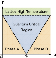
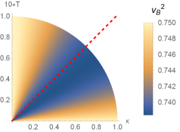
Figure 1: Left: The schematic phase diagram of quantum phase transition. Right: Density plot of butterfly velocity $v_{B}$ in the phase diagram of AdS-AdS domain wall. The red dashed line mark the place where scalar field at the horizon reaches half of its value at IR fixed point. Such line indicate the vague boundary between quantum critical region and non-quantum-critical-region, namely $T$ and $|\kappa|^{z\nu}$ are comparable ($z\nu$ in these two plots is equal to 1). One can compare these two plots by identifying $\kappa\sim g-g_{c}.$

II AdS-Schwarzschild black hole with scalar deformation

In this section we will investigate how the butterfly velocity $v_{B}$ (11) and the charge diffusion ratio $D_{c}\lambda_{L}/v_{B}^{2}$ (12) change under the scalar deformation $W(\cal O_{\phi})$. As the starting point, we consider a classical Einstein gravity theory with the solution of $AdS_{d+2}$ spacetime, which is dual to a large $N$ and strongly coupled theory at conformal fixed point ($z=1$) in $d$ dimensional space. The action of the Einstein-Scalar model is given as

$${\cal S}=\frac{1}{16\pi G_{N}}\int dx^{d+2}\sqrt{-g}\left(R-\frac{1}{2}(\nabla\phi)^{2}-V(\phi)\right),$$ (15)

whose equations of motion are read as

$$0=R_{\mu\nu}-\frac{1}{d}g_{\mu\nu}V(\phi)-\frac{1}{2}\partial_{\mu}\phi\partial_{\nu}\phi,$$ (16a)

$$0=\nabla^{2}\phi-V^{\prime}(\phi).$$ (16b)

For a constant $\phi_{*}$ satisfying $V^{\prime}(\phi_{*})=0$ and $V(\phi_{*})<0$, there is an $AdS_{d+2}$ solution

$$ds^{2}=\frac{L^{2}}{r^{2}}(-dt^{2}+dr^{2}+d\textbf{x}^{2}),\quad-V(\phi_{*})L^{2}=(d+1)d,\quad\phi=\phi_{*},$$ (17)

where $\textbf{x}=(x_{1},x_{2},\cdots,x_{d})$. At finite temperature the bulk geometry can be described by an AdS-Schwarzschild black hole with flat horizon

$$ds^{2}=\frac{L^{2}}{r^{2}}\left(-f(r)dt^{2}+f(r)^{-1}dr^{2}+d\textbf{x}^{2}\right),\quad f(r)=1-\left(\frac{r}{r_{h}}\right)^{d+1},$$ (18)

where $r_{h}$ is the location of the horizon. We have presented the detailed derivation of the holographic butterfly effect and charge diffusion over a general black hole background in Appendix B. According to the horizon formula (73) and (80), the butterfly velocity $v_{B}$ and temperature $T$ are

$$v_{B}^{2}=\frac{d+1}{2d},\quad T=\frac{d+1}{4\pi r_{h}}.$$ (19)

Now we introduce a deformation of the scalar field by turning on its source, which will back-react to the metric. Suppose the potential $V(\phi)$ can be expanded near $\phi=\phi_{*}$ as

$$V(\phi)=V(\phi_{*})+\frac{m^{2}}{2}(\phi-\phi_{*})^{2}+\cdots.$$ (20)

Then the equation of motion for the scalar field leads to the following deformation uniformly

$$\phi=\phi_{*}+\phi_{-}r^{\Delta_{-}}+\cdots+\phi_{+}r^{\Delta_{+}}+\cdots,$$ (21)

where $\Delta_{\pm}=\frac{1}{2}\left(d+1\pm\sqrt{(d+1)^{2}+4m^{2}L^{2}}\right)$. For later convenience, we define a parameter $\vartheta\equiv\frac{\Delta_{-}}{d+1}$. As the calculation presented in Appendix A, the scalar field equation at $O(\phi-\phi_{*})$ give

$$\phi_{+}=\phi_{-}H\left(\vartheta\right)r_{h}^{\Delta_{-}-\Delta_{+}}+O(\phi_{-}^{2}),$$ (22)

where the specific expression of function $H(\vartheta)$ is given in (57). Such a relation is nothing but the Green function of $\cal O_{\phi}$ at the conformal fixed point once the quantization method is specified. The scalar field back-reacts to the metric at order $O((\phi-\phi_{*})^{2})$, and affects $v_{B}$ through the horizon formula (80). We are mainly concerned with the relevant or ‘weakly’ irrelevant deformation, which is subject to the condition $-\frac{1}{2}<\vartheta<\frac{1}{2}$. The result is

$$v_{B}^{2}=\frac{d+1}{2d}\left(1-\phi_{-}^{2}r_{h}^{2\Delta_{-}}I\left(\vartheta\right)\frac{d+1}{2d}\right)+O(\phi_{-}^{3}),$$ (23)

where the specific expression of function $I(\vartheta)$ is given in (60). When $-\frac{1}{2}<\vartheta<\frac{1}{2}$, we find $I(\vartheta)\geq 0$ with the equality only for $\vartheta=0$. It tells us that $v_{B}$ always decreases up to $O(\phi_{-}^{2})$ except for a marginal deformation. It seems this result coincides with the argument presented in Feng:2017wvc , where it is found that AdS-Schwarzschild black hole has the maximal $v_{B}$ in Einstein-Scalar model (15) when entropy is fixed. Nevertheless, we point out in Appendix E that one of their hypotheses in Feng:2017wvc is actually violated in our model, following the perturbation analysis presented in Appendix A.

According to (11), we expect that the second term in (23) can be expressed in terms of the dimensionless source $\kappa$ and the other scale $T$. Firstly, we point out that $T$ is still related to $r_{h}$ by (19) up to $O(\phi_{-})$, since the scalar field does not back-react to the metric at $O(\phi-\phi_{*})$. To ensure this, we obtain the variation of $T$ at $O(\phi_{-}^{2})$ for $0<\vartheta<\frac{1}{2}$ in (64), indicating that it is not important enough to correct $v_{B}$ at $O(\phi_{-}^{2})$, indeed. Secondly, we remark that the identification of $\kappa$ depends on the choice of quantization method as well as the form of the deformation $W(\cal O_{\phi})$. We present our specific consideration as follows.

We first focus on the standard quantization with $[{\cal O}_{\phi}]=\Delta_{+}$. According to the asymptotic expansion (21), the source $\kappa_{s}$ of $W(\cal O_{\phi})$ is identified as Witten:2001ua

$$\phi_{-}=\kappa_{s}W^{\prime}\left((\Delta_{+}-\Delta_{-})\phi_{+}\right),$$ (24)

where the subscript ‘$s$’ of $\kappa_{s}$ denotes the standard quantization.

For single trace deformation $W(\cal O_{\phi})=\cal O_{\phi}$, we have $1/\nu=[\kappa_{s}]=\Delta_{-}$. Such deformation is relevant. From (24), we identify $\kappa_{s}=\phi_{-}$ and obtain

$$v_{B}^{2}=\frac{d+1}{2d}\left(1-\gamma\frac{\kappa_{s}^{2}}{T^{2/\nu}}\right)+O(\kappa_{s}^{3}),$$ (25)

where $\gamma=\frac{(d+1)I\left(\vartheta\right)}{2d}\left(\frac{d+1}{4\pi}\right)^{\frac{2}{\nu}}$. We check our analytical result in (25) by numerically constructing an AdS domain wall at finite temperature in Appendix C. Both relevant and weakly irrelevant cases are well testified.

For double trace deformation $W({\cal O}_{\phi})=\frac{1}{2}{\cal O}_{\phi}^{2}$, we have $[{\cal O}_{\phi}^{2}]=2\Delta_{+}>d+1$ and $1/\nu=[\kappa_{s}]=\Delta_{-}-\Delta_{+}<0$. Such deformation is irrelevant. $\phi_{-}$ is offset in (24) and a critical temperature is obtained as Faulkner:2010gj

$$T_{c}=\frac{d+1}{4\pi}\left(-\frac{H\left(\vartheta\right)\kappa_{s}}{\nu}\right)^{\nu}.$$ (26)

We will see later that the physical meaning of $T_{c}$ becomes more transparent in the alternative quantization.

If $\frac{1}{2}-\frac{1}{d+1}<\vartheta<\frac{1}{2}$, i. e. $\frac{d+1}{2}-1<\Delta_{-}<\frac{d+1}{2}$, we can choose alternative quantization with $[{\cal O_{\phi}}]=\Delta_{-}$. The source $\kappa_{a}$ of $W(\cal O_{\phi})$ is identified by

$$(\Delta_{-}-\Delta_{+})\phi_{+}=\kappa_{a}W^{\prime}\left(\phi_{-}\right),$$ (27)

where the subscript ‘$a$’ of $\kappa_{a}$ denotes alternative quantization.

For single trace deformation $W(\cal O_{\phi})=\cal O_{\phi}$, we have $1/\nu=[\kappa_{a}]=\Delta_{+}$. Such deformation is relevant. We identify $\kappa_{a}=\phi_{+}$ and obtain

$$v_{B}^{2}=\frac{d+1}{2d}\left(1-\gamma\frac{\kappa_{a}^{2}}{T^{2/\nu}}\right)+O(\kappa_{a}^{3}),$$ (28)

where $\gamma=\frac{(d+1)I(\vartheta)}{2dH(\vartheta)}\left(\frac{d+1}{4\pi}\right)^{\frac{2}{\nu}}$.

For double trace deformation $W({\cal O}_{\phi})=\frac{1}{2}{\cal O}_{\phi}^{2}$, we have $[{\cal O}_{\phi}^{2}]=2\Delta_{-}<d+1$ and $1/\nu=[\kappa_{a}]=\Delta_{+}-\Delta_{-}>0$. Such deformation is relevant. Similar to the case of standard quantization, there is a critical temperature

$$T_{c}=\frac{d+1}{4\pi}\left(-\frac{\nu\kappa_{a}}{H\left(\vartheta\right)}\right)^{\nu}.$$ (29)

(29) and (26) become identical as $\kappa_{a}=-1/\kappa_{s}$, which is obtained just by exchanging the source and the expectation value. If $\vartheta>0$, $H<0$ always, then $T_{c}$ is well defined only when $\kappa_{a}<0$. When $\kappa_{a}>0$, double trace deformation does not affect the metric and $v_{B}$, at least at $O(\kappa_{a}^{2})$. It is not surprising since such deformation with $\kappa_{a}>0$ drives a RG flow from the UV fixed point with $[{\cal O}_{\phi}]=\Delta_{-}$ to the IR fixed point with $[{\cal O}_{\phi}]=\Delta_{+}$ Witten:2001ua , but does not affect the geometry classically Gubser:2002zh . To investigate the possible effects of such flow on $v_{B}$, one should further study quantum corrections. However, when one attempts to go to the subleading order with finite $N$, the first term $\frac{d+1}{2d}$ of $v_{B}$ may receive corrections as well, which makes the effect of such flow unclear. When $\kappa_{a}>0$, Faulkner et. al. Faulkner:2010gj ; Faulkner:2010fh found that a new instability at $T\leq T_{c}$, where the scalar field will condensate with a mean-field critical exponent at finite temperature. Then $v_{B}$ will behave just like undergoing the phase transition in a holographic superconductor model, whose derivative is discontinuous at the phase transition point Ling:2016wuy .

Next we turn to investigate the charge diffusion bound (12) in this holographic model. We introduce an electromagnetic term into the action and then consider the perturbations of electromagnetic field $A$

$${\cal S}_{c}=\frac{1}{16\pi G_{N}}\int dx^{d+2}\sqrt{-g}(-\frac{1}{4}F^{2})$$ (30)

where $F$ is the field strength $F=dA$. We calculate the change of $T$ and $D_{c}$ for $\vartheta>0$ in Appendix A and then substitute them into the diffusion ratio (12). For the case of standard quantization and single trace deformation, the result is

$$\frac{D_{c}\lambda_{L}}{v_{B}^{2}}=\Psi(0)\left(1+\eta\frac{\kappa_{s}^{2}}{T^{2/\nu}}\right)+O(\kappa_{s}^{3}),$$ (31)

where

$$\eta=J\left(\vartheta,d\right)\left(\frac{d+1}{4\pi}\right)^{\frac{2}{\nu}},\quad\Psi(0)=\left\{\begin{array}[]{ll}\log\left(\frac{\Lambda_{\text{UV}}}{2\pi T}\right),&\text{ for }d=1\\ \frac{d}{d-1},&\text{ for }d>1\end{array}\right.$$ (32)

and $\Lambda_{\text{UV}}$ is the UV cutoff, which reflects the UV sensitivity of $D_{c}$ at $d=1$ Blake:2016wvh . The expression of $J(\vartheta,d)$ is given in (68) or (69). We have numerically estimated $J(\vartheta,d)$ for a wide range of parameters $(\vartheta,d)$ and found that it is always non-negative. It means that when the system goes away from the quantum critical region, the bound is more solid.

Finally, we may investigate (4) for the momentum transport. In a large, neutral and homogeneous system, according to the thermodynamic relation Gubser:2009cg ; Caldarelli:2016nni

$$\epsilon=Ts-p,$$ (33)

the momentum diffusion constant is Blake:2016wvh

$$D_{p}=\frac{\eta}{\epsilon+p}=\frac{\eta}{Ts}=\frac{1}{4\pi T},$$ (34)

where $\epsilon$ is the energy density and $s$ is the entropy density, while $p$ is the pressure. The saturated KSS bound $\eta/s=1/(4\pi)$ in Einstein gravity is also used. Then its diffusion ratio is

$$\frac{D_{p}\lambda_{L}}{v_{B}^{2}}=\frac{1}{2v_{B}^{2}},$$ (35)

which increases as well when the system goes away from the quantum critical region.

III Lifshitz black hole with scalar deformation

In previous section we have analysed $v_{B}$ and $D_{c}\lambda_{L}/v_{B}^{2}$ in holographic systems with $AdS_{d+2}$ geometry deformed by scalar field. In this section we show that it can be generalized to the Lifshitz case Kachru:2008yh . Lifshitz spacetime can be found in massive vector model Taylor:2015glc ; Taylor:2008tg

$${\cal S}=\frac{1}{16\pi G_{N}}\int dx^{d+2}\sqrt{-g}\left(R-\frac{1}{4}{\cal G}^{2}-\frac{1}{2}W{\cal B}^{2}-\frac{1}{2}(\nabla\phi)^{2}-V(\phi)\right),$$ (36)

where $\cal B$ is a one-form field and ${\cal G}=d{\cal B}$. To study the scalar deformation, we have added a minimally coupled scalar field into the action. It allows a Lifshitz solution

$$\begin{split}&ds^{2}=L^{2}\left(-\frac{dt^{2}}{r^{2z}}+\frac{dr^{2}+d\textbf{x}^{2}}{r^{2}}\right),\quad{\cal B}=L\sqrt{\frac{2(z-1)}{z}}r^{-z}dt,\quad\phi=\phi_{*},\\ &WL^{2}=dz,\quad-V(\phi_{*})L^{2}=z^{2}+z(d-1)+d^{2},\quad V^{\prime}(\phi_{*})=0,\end{split}$$ (37)

where $z$ is the dynamical critical exponent. This solution enjoys a scaling symmetry with scaling dimension $[t]=-z,\,[r]=-1,\,[x]=-1$. It is worthwhile to point out that the Lifshitz solution with massive vector (37) can smoothly go back to the AdS solution (17) if one sets $z=1$, while the Lifshitz solution with running dilaton can not Taylor:2015glc ; Taylor:2008tg .

To study butterfly effect, one should construct a bulk geometry with finite temperature. While, a general analytical Lifshitz black hole with flat horizon in massive vector model has not yet been found Taylor:2015glc . But we still expect the scaling dimension of temperature $[T]=-[t]=z$. For the expansion of potential $V(\phi)$ in (20), the scalar field has the same expansion as (21) but with different scaling dimensions $\Delta_{\pm}=\frac{1}{2}\left(d+z\pm\sqrt{(d+z)^{2}+4m^{2}L^{2}}\right)$. The deformation of the scalar back-react to the metric at $O((\phi-\phi_{*})^{2})$. According to scaling analysis, we expect

$$v_{B}^{2}=T^{2-\frac{2}{z}}\Phi(0)(1-\gamma\frac{\phi_{-}^{2}}{T^{\frac{2\Delta_{-}}{z}}})+O(\phi_{-}^{3})$$ (38)

with two undetermined constants $\Phi(0)$ and $\gamma$. For the case of single trace deformation, we can identify $\kappa=\phi_{-}$ and $1/\nu=\Delta_{-}$. (38) should go back to (25) if we set $z=1$.

In Appendix D, we numerically build a Lifshitz black hole with or without scalar. When scalar field vanishes, we find that $\Phi(0)$ is not equal to $\frac{d+z}{2d}$, which is the coefficient obtained in Lifshitz black hole with running dilaton in Roberts:2016wdl ; Blake:2016wvh . Such discrepancy is not surprising, since Lifshitz black hole with running dilaton is not a solution of (36). When scalar field is turned on, we use standard quantization and impose the boundary conditions on $\phi_{-}$. Indeed, our numerical results match (38) at small $\phi_{-}$ when $0<\Delta_{-}<\frac{d+z}{2}$. The coefficients $\Phi(0)$ and $\gamma$ are shown in Figure 2. Within our observation, $\Phi(0)$ and $\gamma$ are always positive.

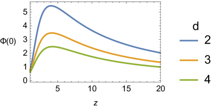
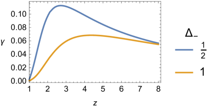
Figure 2: The two coefficients $\Phi(0)$ and $\gamma$ in the expansion (38) as functions of dynamical exponent $z$. In the right plot, spatial dimension is $d=2$.

IV Comments on other phases at low temperature and phase transitions

In this section we will focus on the behavior of $v_{B}$ in some low temperature phases in the non-quantum-critical region $T\ll|\kappa|^{z\nu}$. We demonstrate that no universal behavior is observed in these low temperature phases or holographic BKT transition, which is in contrast with the results for quantum critical region controlled by a single fixed point, as we have investigated in previous sections. In next two subsections, a gapless phase and a gapped phase in the holographic framework with hyperscaling violation (HV) will be investigated. A relevant scalar deformation (21) with standard quantization and single trace deformation can drive the AdS solution (17) from the UV region to these HV solutions in the IR region. We will identify $\kappa=\phi_{-}$ and $1/\nu=\Delta_{-}$, where $\Delta_{-}>0$ is required for a relevant deformation. In the last subsection, a holographic model with quantum BKT phase transition is discussed.

IV.1 Gapless phase with hyperscaling violation

In the Einstein-Scalar model (15), we choose the asymptotic behavior of the potential $V(\phi)$ at $\phi\to\infty$ as

$$V(\phi\to\infty)\sim V_{0}e^{\alpha\phi}(1+V_{1}e^{\alpha_{1}\phi}),$$ (39)

in order to construct a AdS-HV domain wall from $\phi=\phi_{*}$ to $\phi\to\infty$. The term $V_{1}$ is common in the UV completion of HV geometry where the scalar $\phi$ serves as the dilaton Kiritsis:2015oxa ; Gouteraux:2012yr ; Charmousis:2010zz . We can heat up the system to finite but low temperature $T\ll|\kappa|^{\nu}$ by perturbing a small HV black hole in the IR

$$\begin{split}ds^{2}&=L_{\text{HV}}^{2}r^{\frac{2\theta}{d}-2}(1+g_{1}r^{\delta}+\cdots)\left[-\left(1-c_{T}r^{d-\theta+1}+\cdots\right)dt^{2}+\left(1+c_{T}r^{d-\theta+1}+\cdots\right)dr^{2}+d\textbf{x}^{2}\right],\\ e^{\phi}&=r^{\epsilon}(1+\phi_{1}r^{\delta}+\cdots),\end{split}$$ (40)

where

$$\alpha\epsilon=-\frac{2\theta}{d},\quad\epsilon^{2}=-\frac{2\theta}{d}(d-\theta),\quad\delta=\alpha_{1}\epsilon,\quad-V_{0}L_{\text{HV}}^{2}=(d-\theta)(d-\theta+1).$$ (41)

The region of $0<\theta\leq d+1$ is excluded by the requirement of relevant thermal mode $c_{T}$ and Null Energy Condition Gouteraux:2012yr . When $\theta>d+1$, the solution is found to be gapped and thermodynamically unstable Liu:2013una ; Kiritsis:2015oxa . We will discuss this in the next subsection. In this subsection, we focus on the case of $\theta<0$, where the solution is found to be gapless and thermodynamically stable Liu:2013una ; Kiritsis:2015oxa ; Dong:2012se . The IR is located at $r\xrightarrow{IR}+\infty$, where the induced line element vanishes. There are two perturbation modes in (40), whose coupling is approximately negligible if they are small enough. The mode of $\{g_{1},\phi_{1}\}$ is generated by the second term $V_{1}$ in (39), where the coefficients $\{g_{1},\phi_{1}\}$ can be solved in the series expansion about $V_{1}$. The mode of $c_{T}$ corresponds to perturbing a small black hole with horizon $r_{h}=c_{T}^{\frac{1}{d-\theta+1}}$ and temperature $T=\frac{|d-\theta+1|}{4\pi r_{h}}$. We find that above two modes are most important to the variation of $v_{B}$. One can consider other modes in (40), and will find that their scaling dimensions are $0$ or $d-\theta+1$ Gouteraux:2012yr . Except for the thermal mode of $c_{T}$, all the relevant modes should not be stimulated for a stable HV solution in the IR. The marginal modes could be introduced but they only provide secondary contribution to $v_{B}$ when compared with two modes in (40).

Plugging (40) into the horizon formula of $v_{B}$ (80), we obtain $v_{B}$ up to the subleading order

$$v_{B}^{2}\approx\frac{d-\theta+1}{2(d-\theta)}\left(1+\frac{d\delta}{2(d-\theta)}g_{1}r_{h}^{\delta}\right)=\frac{d-\theta+1}{2(d-\theta)}\left(1+\gamma\left(\frac{\kappa^{\nu}}{T}\right)^{\delta}\right),\quad T\ll|\kappa|^{z\nu},$$ (42)

where the approximate equality is used since we neglect the coupling between these two modes of perturbations. This final result is obtained based on the following analysis. In the UV ($r\to 0$), $\phi$ is expanded as (21). One can find the scaling relation $\kappa^{\nu}=\phi_{-}^{1/\Delta_{-}}=Z_{g}g_{1}^{1/\delta}$ where $Z_{g}$ is a constant which can not be determined by scaling analysis but relies on the specific form of the potential $V(\phi)$. Then we obtain the final result of (42) with constant $\gamma=\frac{d\delta}{2(d-\theta)}\left(\frac{|d-\theta+1|}{4\pi Z_{g}}\right)^{\delta}$. The power $\delta$ in (42) is somehow not a universal quantity, since it relies on the second exponent $\alpha_{1}$ of $V(\phi)$ in (39), which is a tail of the UV completion process.

IV.2 Gapped phase with hyperscaling violation

Now we come to the case of $\theta>d+1$. In this case the IR of (40) is located at $r\xrightarrow{IR}0$. The entropy density $s$ over the background in (40) behaves as $s\sim T^{d-\theta}$, leading to a negative specific heat such that the HV black hole is thermodynamically unstable Gursoy:2008za ; Kiritsis:2015oxa ; Ling:2016ien . Here we numerically study the AdS-HV domain wall in $d=2$ with potential $V(\phi)=-6-3\sinh^{2}\left(\frac{\phi}{\sqrt{3}}\right)$. In the UV, the domain wall approaches the AdS spacetimes with $L=1$, $\Delta_{-}=1$ and $\Delta_{+}=2$. While in the IR, it approaches the HV geometry with $\theta=8$.

To study the thermodynamics of the system, we should heat it up and calculate its free energy density $f$. Firstly, from holographic renormalization Skenderis:2002wp ; Caldarelli:2016nni , one notices that the trace of energy momentum tensor is $-\epsilon+2p=\langle T^{i}{}_{i}\rangle=\phi_{-}\phi_{+}$ . Thus, according to the thermodynamic relation (33) and $f=\epsilon-Ts$, we obtain the expression of free energy density as

$$f=-\frac{1}{3}(Ts+\phi_{-}\phi_{+}).$$ (43)

We skip the details of numerical analysis since it is similar to the case of AdS-AdS domain wall as presented in Appendix C. We construct dimensionless quantities with the unit of $\kappa=\phi_{-}$. The temperature dependence of the dimensionless free energy density $f/\kappa^{3}$ and the butterfly velocity $v_{B}^{2}$ are shown in Figure 3. We find two branches of black hole solutions and a branch of thermal gas solutions. The branch of big black holes behaves like the AdS-Schwarzschild black hole (18) with positive specific heat and $v_{B}^{2}\leq\frac{d+1}{2d}=\frac{3}{4}$. While, the branch of small black holes behaves like the HV black hole (40) with negative specific heat and $v_{B}^{2}\geq\frac{d-\theta+1}{2(d-\theta)}=\frac{5}{12}$. It becomes extremal at $T/\kappa\to\infty$. There is a minimal dimensionless temperature $\tilde{T}_{\text{min}}$ for those branches of black holes. The branch of thermal gases has the same form of the extremal solution but has compact imaginary time $\tau\sim\tau+T^{-1}$ Gursoy:2008za ; Kiritsis:2015oxa . A critical temperature $\tilde{T}_{c}$ which is higher than $\tilde{T}_{\text{min}}$ appears at the intersection between the branch of big black holes and the branch of thermal gases in the plot of free energy density. The thermal gas dominates when $T/\kappa<\tilde{T}_{c}$ while the big black hole dominates when $T/\kappa>\tilde{T}_{c}$. So a first-order phase transition occurs at $\tilde{T}_{c}$.

Specifically, a holographic description of chaos is ill-defined in thermal gas phase since horizon is absent. So when $T/\kappa$ decreases and the system falls into such gapped phase with HV, chaos may disappear and $v_{B}$ becomes ill-defined when $T/\kappa<\tilde{T}_{c}$.

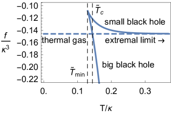
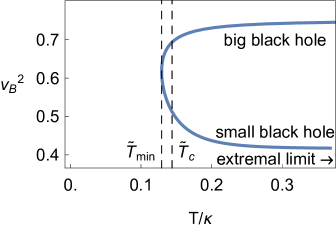
Figure 3: Dimensionless free energy density $f/\kappa^{2}$ and butterfly velocity $v_{B}^{2}$ as function of dimensionless temperature $T/\kappa$ for gapped phase with $d=2,\theta=8$. In the left plot, black hole solutions are represented by solid line, thermal gas solution are represented by dashed line.

IV.3 Holographic Berezinskii-Kosterlitz-Thouless transition

Now we consider a holographic BKT transition which goes beyond the quantum criticality discussed above, whose QCP is so-called bifurcating QCP Kaplan:2009kr ; Iqbal:2010eh ; Jensen:2010ga ; Iqbal:2011ae ; Evans:2010hi ; Iqbal:2011aj ; Jensen:2010vx . From the perspective of RG flow, holographic BKT transition is the result of the annihilation between two fixed points which are linked by the double-trace flow mentioned in section II. Consider a scalar field $\phi$ in the bulk and the source of its dual operator $\cal O_{\phi}$ in the boundary theory is set to zero. Consider an $AdS_{n}$ scaling geometry at zero temperature, when one tunes the effective mass $m_{\text{eff}}$ of $\phi$ to become lower than its BF bound $m_{\text{BF}}$ with respect to $AdS_{n}$, two fixed points which are respectively dual to the $AdS_{n}$ with standard quantization and alternative quantization will merge and then annihilate Kaplan:2009kr . Then $\phi$ will condense spontaneously and display a nonzero expectation value $\langle\cal O_{\phi}\rangle$. The condensation of $\phi$ generates an intrinsic IR scale $\Lambda_{\text{IR}}$ which exhibits a BKT scaling Kaplan:2009kr ; Jensen:2010ga ; Iqbal:2010eh

$$\Lambda_{\text{IR}}\sim\Lambda_{\text{UV},n}e^{-\pi/\tilde{\alpha}},\quad\tilde{\alpha}=L_{n}\sqrt{m_{\text{BF}}^{2}-m_{\text{eff}}^{2}},$$ (44)

where $\Lambda_{\text{UV},n}$ and $L_{n}$ are the UV cutoff and the radius of the $AdS_{n}$, respectively. A BKT scaling is found in the condensation $\langle{\cal O}_{\phi}\rangle\sim\Lambda_{\text{UV},n}^{\Delta}e^{-\pi/(2\tilde{\alpha})}$ as well, where $\Delta$ is the scaling dimension of operator ${\cal O}_{\phi}$. So such transition is infinite order and is called holographic BKT transition. The bifurcating QCP is located at $\tilde{\alpha}=0$.

However, when the system goes to finite temperature $T$, the transition becomes the second order with critical value $\tilde{\alpha}_{c}=\pi\log^{-1}\left(\frac{\Lambda_{\text{UV},n}}{T}\right)$ and mean field exponent $\langle{\cal O}_{\phi}\rangle\sim\left(\tilde{\alpha}-\tilde{\alpha}_{c}\right)^{\frac{1}{2}}$ Jensen:2010ga .

Usually once a bulk action is given, then the mass $m$ of the bulk field $\phi$ is fixed. What we can tune in a QPT is the source of the operators in the dual QFT. Actually, the effective mass $m_{\text{eff}}$ can be tuned by adjusting the fields which are coupled to $\phi$ Iqbal:2010eh ; Jensen:2010ga ; Jensen:2010vx . For instance, one can consider a coupling term $\int d^{d+1}x\sqrt{-g}\frac{1}{2}Y(\psi)\phi^{2}$ in the bulk action, where $\psi$ is a massless axion field and $Y(\psi)$ is a function. The IR value $\psi_{\text{IR}}$ of the axion field $\psi$ could be controlled by the source $\psi_{s}$ of its dual operator. Such coupling term will contribute to the effective mass as $m_{\text{eff}}^{2}=m^{2}-Y(\psi_{\text{IR}})$. So the relation between $m_{\text{eff}}$ and $\psi_{s}$ depends on the detail of function $Y(\psi)$. Consequently, by tuning the source $\psi_{s}$, one can adjust $m_{\text{eff}}$ and trigger a BKT transition according to the mechanism given above. For instance, some BKT transitions can be triggered by tuning magnetic fields which lead to condensation of scaler fields on $AdS_{2}\times R^{d}$ geometries in the IR Jensen:2010ga ; Evans:2010hi ; Jensen:2010vx .

To further consider the butterfly velocity $v_{B}$ near the BKT transition, we should study the system at finite temperature. Firstly, we discuss the behavior of $v_{B}$ when approaching such bifurcating QCP from the uncondensed phase. According to the horizon formula of $v_{B}$ (80), one should investigate the full backreactions of $\psi$ to the metric. The effects of such backreactions depend on the potential of $\psi$ and its couplings with other fields. We expect a complicated behavior which is different from the simple form (23). Especially, a universal maximization of $v_{B}$ near QCP will not appear, since one can easily shift the location of QCP by changing $Y(\psi)$ while leaving the metric as well as the butterfly velocity $v_{B}$ unchanged in the uncondensed phase.

Next we consider the system undergoes the phase transition and then enters the condensed phase. Since the phase transition has mean-field scaling at finite temperature, which is just like a holographic superconductor transition, we expect that a discontinuity of $\partial v_{B}/\partial\tilde{\alpha}$ will appear at the phase boundary Ling:2016wuy .

In addition, when $m_{\text{eff}}^{2}>m_{\text{BF}}^{2}$, there is a double-trace flow between the fixed points with standard quantization and alternative quantization. While, as is discussed in section II, such flow does not back-react to the metric and $v_{B}$ classically.

V Comparisons with the results in many-body system

In this section we are going to compare our results in holographic approach with the ones obtained in many body system, including $d=1$ Bose-Hubbard model (BHM) and $d=2$ $O(N)$ nonlinear sigma model with large $N$ Shen:2016htm ; Bohrdt:2016vhv ; Chowdhury:2017jzb .

V.1 Bose-Hubbard model

With the use of numerical simulation, the OTOC (3) near the tip of the Mott insulating lob with density $\rho=1$ has been computed in Shen:2016htm ; Bohrdt:2016vhv . There is a Mott insulator-superfluid transition at $U/J\approx 3.4$, where $U$ measures the in-site repulsion energy and $J$ measures the nearest-neighbor hopping energy. Mott insulating phase falls in the region with $U/J>3.4$ while superfluid phase falls in $U/J<3.4$. It is known that such kind of transition is a BKT type which belongs to the universal class of $O(2)$ model in $d=1$ Sachdev:1999QPT . The field theory version of such BKT transition is sine-Gordon model where the mergence and annihilation between two fixed points at the QCP is found Kaplan:2009kr . Actually, from the perspective of RG flow, such BKT transition is controlled by a line of fixed points rather than a single fixed point Sachdev:1999QPT . A gap with BKT scaling (44) appears in Mott insulating phase.

Nevertheless, so far a clear duality between the BKT transition in BHM and the holographic BKT transition has yet been found. Some difficulties arise when one attempts to compare the butterfly effect in these two different scenarios. Firstly, the mean-field scaling at finite temperature in holographic BKT is different from that one in the BKT transition of many-body system. Secondly, as discussed in subsection IV.3, before two fixed points annihilate, the double-trace flow continuously changes. But such change does not affect the metric at classical level, let alone the butterfly effect. So, as a preliminary approach, we attempt to provide a phenomenological view on this issue by comparing the results (13) and (14) in the second order QPT with the ones in above Bose-Hubbard model.

In Shen:2016htm , the authors considered a system with $7$ sites and $7$ bosons and applied the method of exact diagonalization. The system goes across the QCP by tuning the $U/J$ at fixed and finite temperature. The result of butterfly velocity $v_{B}$ is shown in Figure 4, where a peak of $v_{B}$ near $U/J\approx 9$ is observed. Such value $U/J\approx 9$ is larger than the critical value $U/J\approx 3.4$ at zero temperature. It was conjectured in Shen:2016htm that such deviation may be ascribed to finite temperature and finite size. In spite of the deviation, the phenomenon found in this many body system is analogous to our holographic results (13) with fixed $T$.

In Bohrdt:2016vhv , the authors perform the numerical simulations based on matrix-product-operators at finite-temperature. The system size is large enough to guarantee the convergence. The result of butterfly velocity $v_{B}$ is shown in Figure 5. Let us focus on the case of $U=3J$ where the system is close to QCP at zero temperature. When $T\gg J$, as shown in Figure 5, the system falls in the region of lattice high temperature and the scaling symmetry does not emerge. When $T\lesssim J$, the system lies in quantum critical region. In such region, as $T/J$ goes down, $v_{B}$ begins to decrease, which coincides with the tendency of our holographic results (13) with fixed $\kappa$.

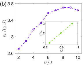
Figure 4: Butterfly velocity $v_{B}$ as a function of coupling $U/J$ at temperature $\beta J=0.9$. This plot is taken from Shen:2016htm .

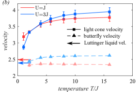
Figure 5: Butterfly velocity $v_{B}$ as a function of temperature $T/J$ for different coupling $U/J$. This plot is taken from Bohrdt:2016vhv .

V.2 $O(N)$ nonlinear sigma model

Let us turn to the $d=2$ $O(N)$ nonlinear sigma model. In Chowdhury:2017jzb , the authors studied the chaos with QPT up to $1/N$ order. The QCP at $g=g_{c}$ and $T=0$ is controlled by a $z=1$ CFT. In the quantum critical region, they focus on $g=g_{c}$ and only consider the dominating scale $T$. The inverse phase coherent time is $\frac{1}{\tau_{\varphi}}=1.152\frac{T}{N}$, which is suppressed by large $N$. Then quasi-particles are still well defined up to $1/N$ order Sachdev:1999QPT . The dispersion relation at $N=\infty$ is

$$\epsilon_{\bm{k}}^{2}=c^{2}{\bm{k}}^{2}+\mu^{2},$$ (45)

where the speed of light $c=1$, the thermal mass $\mu=\Theta T$ and the constant $\Theta=2\log\frac{1+\sqrt{5}}{2}$. The thermal mass $\mu$ gives a finite correlation length $\xi=1/\mu$ at $N=\infty$ .

To study the quantum chaos, the authors in Chowdhury:2017jzb consider the interaction up to $1/N$. By calculating the square commutator (1), they extract the Lyapunov exponent and the butterfly velocity, which are $\lambda_{L}\approx 3.2\frac{T}{N}$ and $v_{B}\approx c$. The Lyapunov exponent $\lambda_{L}$ is suppressed by large $N$ and the butterfly velocity $v_{B}$ is closed to the specific velocity of quasi-particle. Both of $\lambda_{L}$ and $v_{B}$ are different from the ones in gravity. It is reasonable, since the dual field theory of Einstein gravity is considered as large $N$ gauge field theories at strong coupling.

To discuss the behavior of $v_{B}$ in the quantum critical region, as what is done in above sections, we should deviate the system from the QCP and consider another scale $g-g_{c}$. It generates the energy gap $\Delta_{E}^{\pm}$, where $\Delta_{E}^{-}\sim(g_{c}-g)^{\nu}$ for $g\leq g_{c}$ and $\Delta_{E}^{+}\sim(g-g_{c})^{\nu}$ for $g\geq g_{c}$ and the critical exponent $\nu=1$. Remind that $\kappa\sim g-g_{c}$, we have $\Delta_{E}^{\pm}\sim|\kappa|^{\nu}$ as usual. The energy gap $\Delta_{E}^{\pm}$ only affects the thermal mass $\mu$ with the scaling formulas at $N=\infty$ Sachdev:1999QPT

$$\mu=\left\{\begin{array}[]{lll}2T\sinh^{-1}\left[\frac{1}{2}\exp(-2\pi\Delta_{E}^{-}/T)\right]&\text{ for }&g\leq g_{c}\\ 2T\sinh^{-1}\left[\frac{1}{2}\exp(\Delta_{E}^{+}/2T)\right]&\text{ for }&g\geq g_{c}\end{array}\right.,$$ (46)

both of which match $\mu=\Theta T$ at $g=g_{c}$. From (46), $\mu/T$ monotonously decreases when $g$ increases. So the point $g=g_{c}$ is not an extreme point of $\mu/T$. The energy gap $\Delta_{E}^{\pm}$ does not explicitly enter the calculations of $\tau_{\varphi},\lambda_{L}$ and $v_{B}$ in Chowdhury:2017jzb , except changing the thermal mass $\mu$. The value of $\mu/T=\Theta=2\log\frac{1+\sqrt{5}}{2}$ at $g=g_{c}$ is not special in the calculations of $\tau_{\varphi},\lambda_{L}$ and $v_{B}$, so we do not expect that any extremal behavior of $\tau_{\varphi},\lambda_{L}$ and $v_{B}$ would appear at $g=g_{c}$.

In fact, in the quantum critical region, the saturation of the bound for $\tau_{\varphi}$ in (9) does not guarantee the minimization of $\tau_{\varphi}$ at $g=g_{c}$. If the absence of extreme for $v_{B}$ at $g=g_{c}$ in such model is actually true, it is different from the result of our holographic calculation. It means that the extreme for $v_{B}$ may only appear in the model which has quasi-particle description and weakly chaotic behavior. So we expect to find universal behavior of $v_{B}$ in strong chaotic systems. The complicated dependence of (46) on two scales $T$ and $\Delta_{E}^{\pm}$ implies that, in a many-body system, the finite temperature effects in quantum critical region may not be so simple as that in a holographic system with black holes deformed by a scalar field.

VI Discussion

In this paper, we have investigated the butterfly velocity $v_{B}$ and the diffusion ratios $D_{c,p}\lambda_{L}/v_{B}^{2}$ near the quantum phase transition in holographic approach. In the quantum critical region, when the relevant scalar deformation is turned on, butterfly velocity $v_{B}$ universally decreases such that a local peak of $v_{B}$ is observed near QCP, whose universal behavior depends on the critical exponents and the dimension of the system. In addition, the diffusion ratios $D_{c,p}\lambda_{L}/v_{B}^{2}$ universally increase, which satisfies the diffusion bound (4). We have also studied the behavior of $v_{B}$ in low temperature phases beside the QCP, which is controlled by the IR fixed points. For the gapless phase with running dilaton and hyperscaling violation, the variation of $v_{B}$ mainly relies on the UV completion process, which is not intrinsic. For the gapped phase, black hole does not dominate at low temperature and chaos disappears. In the holographic BKT transition, the behavior of $v_{B}$ relies on the details of the coupling term in the bulk.

The numerical results in BHM support our holographic observation that $v_{B}$ decreases when the system goes away from $g=g_{c}$ but still within the quantum critical region. So we expect that this decreasing behavior of $v_{B}$ is not an occasional phenomenon.

It is instructive to understand the universality of $v_{B}$ in quantum critical region from a theoretical point of view. On gravity side, it seems that one may link it to the well-known holographic C-theorem Freedman:1999gp . But their connections actually are not evident. Firstly, central charge, which is related to the AdS radius $L$, does not appear in the expression of $v_{B}$. Secondly, $v_{B}$ does not monotonously decrease when deformed away from the QCP in the whole phase diagram of QPT. As illustrated in the context of the AdS-AdS domain wall, $v_{B}$ decreases firstly and then increases again as $T/\kappa$ decreases, where the low temperature phase is gapless and controlled by another CFT. Finally, the value of $v_{B}$ at low $T/\kappa$ is the same as the one at high $T/\kappa$. Similar phenomenon is observed in the $O(N)$ nonlinear sigma model in Chowdhury:2017jzb , where the values of $v_{B}$ in the quantum critical region with $g=g_{c}$ and in the symmetry broken phase are the same, although the crossover behavior has not been obtained. Another possible reason for the decrease of $v_{B}$ in quantum critical region is the reverse isoperimetric inequality, which is proposed to be linked to a maximum of $v_{B}$ in Feng:2017wvc . In Appendix E, we find that such inequality is true in our perturbation analysis.

On field theory side, the similarity between (10) and (13) hints the mechanism that the energy gap $\Delta_{E}$ hinders the spread of the chaos even in a system without quasi-particle. While, the discussion about the $O(N)$ nonlinear sigma model tells us that such decrease of $v_{B}$ may not be always true when quasi-particle description is still valid and the chaos is suppressed. Based on the calculation in Chowdhury:2017jzb , the coupling constant $\kappa\sim g-g_{c}$ affects the chaos only through the thermal mass $\mu$. So we expect a detailed discussion about the dependence of chaos on general $\mu$.

Essentially, the BKT transition in BHM is controlled by a fixed line rather than a single fixed point with relevant deformation. The butterfly effect in other QPTs deserve to be further studied, such as the Mott insulator-superfluid transition with fixed density in BHM at $d\geq 2$. Perhaps one more direct way of studying $v_{B}$ under deformation lies on field theory side, such as a generalized SYK model with relevant deformation Gu:2016oyy ; Stanford:2015owe ; Roberts:2014ifa ; Lucas:2017dqa .

Finally, we remark that for simplicity only scalar deformation is considered in this paper. It directly leads to a $\kappa^{2}$-variation of $v_{B}$ and $D_{c,p}\lambda_{L}/v_{B}^{2}$ for single trace deformation, since scalar field usually back-reacts to the metric at second order. It is desirable to explore the possible new features of holographic butterfly effect by considering other kinds of deformations in future. Furthermore, in this paper all the holographic setup is considered only at the classical level, which is dual to a gauge field theory with $N=\infty$. When the subleading order with $1/N$ corrections is taken into account, it is expected that the dependent behavior of $v_{B}$ on $\kappa^{2}$ would receive corrections as well. Last but not least, only Einstein gravity with minimally coupled scalar field is considered in this paper. More general coupling terms such as $f(\phi)R$ or higher order curvature corrections deserve further investigations Roberts:2014isa ; Alishahiha:2016cjk ; Qaemmaqami:2017bdn .

Appendix A Scalar deformation on perturbation

In this appendix we will consider the scalar perturbation over the AdS-Schwarzschild black hole (18) with the action (15). We start with the ansatz for the metric

$$ds^{2}=-E(r)dt^{2}+B(r)dr^{2}+C(r)d\textbf{x}^{2},\quad\phi=\phi(r).$$ (47)

Then we obtain the equations of motion and zero-energy constraint

$$0=\frac{\left(E^{\prime}\right)^{2}}{4BE^{2}}+\frac{B^{\prime}E^{\prime}}{4B^{2}E}-\frac{dC^{\prime}E^{\prime}}{4BCE}-\frac{V(\phi)}{d}-\frac{E^{\prime\prime}}{2BE},$$ (48a)

$$0=\frac{d\left(C^{\prime}\right)^{2}}{4BC^{2}}+\frac{dB^{\prime}C^{\prime}}{4B^{2}C}+\frac{\left(E^{\prime}\right)^{2}}{4BE^{2}}+\frac{B^{\prime}E^{\prime}}{4B^{2}E}-\frac{V(\phi)}{d}-\frac{\left(\phi^{\prime}\right)^{2}}{2B}-\frac{dC^{\prime\prime}}{2BC}-\frac{E^{\prime\prime}}{2BE},$$ (48b)

$$0=\frac{dC^{\prime}\phi^{\prime}}{2BC}+\frac{E^{\prime}\phi^{\prime}}{2BE}-\frac{B^{\prime}\phi^{\prime}}{2B^{2}}+\frac{\phi^{\prime\prime}}{B}-V^{\prime}(\phi),$$ (48c)

$$0=-\frac{d\left(C^{\prime}\right)^{2}}{4BC^{2}}-\frac{C^{\prime}E^{\prime}}{2BCE}+\frac{\left(C^{\prime}\right)^{2}}{4BC^{2}}+\frac{\left(\phi^{\prime}\right)^{2}}{2Bd}-\frac{V(\phi)}{d},$$ (48d)

where the derivative of $\{E,B,C,\phi\}$ is with respect to $r$ while the derivative of $V$ is with respect to $\phi$.

For convenience, we take the coordinate transformation $\zeta=1-f(r)=(r/r_{h})^{d+1}$ such that in coordinates system $\{t,\zeta,\textbf{x}\}$ equation (18) can be written into the form as (47), with components

$$E(\zeta)=(1-\zeta)C(\zeta)=\frac{L^{2}}{r_{h}^{2}}(1-\zeta)\zeta^{-\frac{2}{d+1}},\quad B(\zeta)=\frac{L^{2}}{(d+1)^{2}(1-\zeta)\zeta^{2}}.$$ (49)

where the asymptotic boundary is located at $\zeta\to 0$ and the horizon is at $\zeta=1$.

Now we turn on the deformation of scalar field as presented in (21), then the black hole will be back-reacted by the scalar field. We write such variation into the series expansion of $\lambda$

$$E(\zeta) =\frac{L^{2}}{r_{h}^{2}}(1-\zeta)\zeta^{-\frac{2}{d+1}}(1+\lambda E_{1}(\zeta)+\lambda^{2}E_{2}(\zeta)+\cdots),$$ (50a)

$$B(\zeta) =\frac{L^{2}}{(d+1)^{2}(1-\zeta)\zeta^{2}}(1+\lambda B_{1}(\zeta)+\lambda^{2}B_{2}(\zeta)+\cdots),$$ (50b)

$$C(\zeta) =\frac{L^{2}}{r_{h}^{2}}\zeta^{-\frac{2}{d+1}}(1+\lambda C_{1}(\zeta)+\lambda^{2}C_{2}(\zeta)+\cdots),$$ (50c)

$$\phi(\zeta) =\phi_{*}+\lambda\phi_{1}(\zeta)+\lambda^{2}\phi_{2}(\zeta)+\cdots,$$ (50d)

with the coordinate relation $\zeta=(r/r_{h})^{d+1}$ unchanged. We require that the location of both boundary and horizon should not be changed by the deformation at higher orders. We adopt the gauge

$$E_{i}(\zeta)=C_{i}(\zeta),\quad\text{for}\quad i=1,2,\cdots.$$ (51)

The variation of the scalar field only appears in Einstein equations at $O(\lambda^{2})$. The first order deformation of metric is

$$E_{1}(\zeta)=C_{1}(\zeta)=c_{1}-\frac{c_{2}}{(1+d)\zeta},\quad B_{1}(\zeta)=c_{2}(\frac{1}{2}-\frac{1}{\zeta}).$$ (52)

where $c_{1}$ and $c_{2}$ are two integral constants. $c_{1}$ corresponds to rescaling $t$ and x which should be set to zero to fix the coordinates of the dual field theory. $c_{2}$ controls an irrelevant mode, which should be set to zero as well for preserving the $AdS$ in the UV. Then

$$E_{1}(\zeta)=B_{1}(\zeta)=C_{1}(\zeta)=0.$$ (53)

The scalar equation at $O(\lambda)$ is

$$(1-\zeta)\phi_{1}^{\prime\prime}-\phi_{1}^{\prime}+\frac{(1-\vartheta)\vartheta}{\zeta^{2}}\phi_{1}=0,$$ (54)

where $\vartheta=\frac{\Delta_{-}}{d+1}$ and $\Delta_{\pm}=\frac{1}{2}\left(d+1\pm\sqrt{(d+1)^{2}+4m^{2}L^{2}}\right)$. Here we only study the situation that Breitenlohner-Freedman (BF) bound is satisfied, then $\vartheta<\frac{1}{2}$. The violation of BF bound leads to a holographic Berezinskii-Kosterlitz-Thouless transition in subsection IV.3. $\phi_{1}$ should be regular at the horizon. The solution up to a constant factor is

$$\phi_{1}(\zeta)=\zeta^{\vartheta}\,_{2}F_{1}(\vartheta,\vartheta;2\vartheta;\zeta)-\zeta^{1-\vartheta}\frac{\Gamma(1-\vartheta)^{2}\Gamma(2\vartheta)}{\Gamma(2-2\vartheta)\Gamma(\vartheta)^{2}}\,_{2}F_{1}(1-\vartheta,1-\vartheta;2-2\vartheta;\zeta),$$ (55)

where ${}_{2}F_{1}(a,b;c;\zeta)$ is the Gaussian hypergeometric function. Near $\zeta\to 0$, $\phi_{1}$ is expanded as

$$\begin{split}\phi_{1}(\zeta)\sim\zeta^{\vartheta}+\cdots+H(\vartheta)\zeta^{1-\vartheta}+\cdots=\left(\frac{r}{r_{h}}\right)^{\Delta_{-}}+\cdots+H(\vartheta)\left(\frac{r}{r_{h}}\right)^{\Delta_{+}}+\cdots,\end{split}$$ (56)

where

$$H(\vartheta)=-\frac{\Gamma(1-\vartheta)^{2}\Gamma(2\vartheta)}{\Gamma(2-2\vartheta)\Gamma(\vartheta)^{2}}.$$ (57)

The mode led by $\zeta^{\vartheta}$ is relevant when $\vartheta>0$ while irrelevant when $\vartheta<0$. The mode led by $\zeta^{1-\vartheta}$ is always relevant. We have restored the asymptotic expansion of $\phi_{1}(\zeta)$ with the $r$ coordinate in order to display the $r_{h}$ dependence. By comparing (56) with (21), we can identify $\lambda=\phi_{-}r_{h}^{-\Delta_{-}}=\phi_{+}H(\vartheta)r_{h}^{-\Delta_{+}}$ at $O(\lambda)$ and obtain (22). At $\zeta=1$,

$$\phi_{1}(1)=\frac{2\pi\cot(\pi\vartheta)\Gamma(2\vartheta)}{\Gamma(\vartheta)^{2}}.$$ (58)

Now we consider the perturbations at the subleading order $O(\lambda^{2})$. The Einstein equations at $O(\lambda^{2})$ are differential equations for metric $E_{2},B_{2},C_{2}$ with source $\phi_{1}$ where $\phi_{2}$ is absent. The deformation of metric is found to be

$$C_{2}^{\prime}(\zeta)=E_{2}^{\prime}(\zeta)=\frac{1}{d+1}B_{2}^{\prime}(\zeta)=\frac{1}{d\zeta^{2}}\left(\int_{\zeta}^{1}y^{2}\phi^{\prime}_{1}(y)^{2}\,dy-c_{3}\right).$$ (59)

Similar to the step in (52), we demand that the boundary mode $B_{2}\sim\#\zeta^{-1}$ vanishes, which determines the constant $c_{3}$ to be

$$I(\vartheta)=\int_{0}^{1}y^{2}\phi^{\prime}_{1}(y)^{2}\,dy,$$ (60)

which is a function of $\vartheta$ and plotted in Figure 6. According to the asymptotic expansion (56), integral $I(\vartheta)$ diverges when $\vartheta<-\frac{1}{2}$, which makes such cancellation subtle. However, here we only consider the case of relevant or ‘weakly’ irrelevant deformation. So we assume $-\frac{1}{2}<\vartheta<\frac{1}{2}$ from now on. By setting $c_{3}=I(\vartheta)$, we obtain

$$C_{2}^{\prime}(\zeta)=E_{2}^{\prime}(\zeta)=\frac{1}{d+1}B_{2}^{\prime}(\zeta)=-\frac{1}{d\zeta^{2}}I_{1}(\zeta;\vartheta),$$ (61)

where $I_{1}(\zeta;\vartheta)=\int_{0}^{\zeta}y^{2}\phi^{\prime}_{1}(y)^{2}\,dy\sim\frac{\vartheta^{2}}{2\vartheta+1}\zeta^{2\vartheta+1}$ near $\zeta\to 0$. Obviously, $I(\vartheta)=I_{1}(1;\vartheta)$.

Now, we can calculate the variation of $v_{B}$ according to (80). By using (51) (53) and (61), it is enough to derive it as

$$v_{B}^{2}=\frac{d+1}{2d}\left(1-\lambda^{2}I(\vartheta)\frac{(d+1)}{2d}\right)+O(\lambda^{3}),$$ (62)

which is (23).

On the asymptotic boundary, $\zeta\to 0$, the deformation of the metric behaves as $\zeta^{2\vartheta}$, which is vanishing when $0<\vartheta<\frac{1}{2}$ and divergent when $\vartheta<0$. From now on, we only discuss the case of $0<\vartheta<\frac{1}{2}$. By applying zero-energy constraint (48d) at $O(\lambda^{2})$ on $\zeta\to 0$ and requiring that constant modes of $C_{2},E_{2},B_{2}$ vanish, we can obtain

$$C_{2}(\zeta)=E_{2}(\zeta)=\frac{1}{d+1}B_{2}(\zeta)=-\frac{1}{d}\int_{0}^{\zeta}y^{-2}I_{1}(y;\vartheta)dy\equiv-\frac{1}{d}I_{2}(\zeta;\vartheta).$$ (63)

According to (73), the Hawking temperature $T$ is

$$T=\frac{d+1}{4\pi r_{h}}\left(1+\frac{\lambda^{2}}{2}I_{2}(1;\vartheta)\right)+O(\lambda^{3}).$$ (64)

By combining (62), (73) and (74), we obtain

$$\frac{v_{B}^{2}}{\lambda_{L}}=\frac{r_{h}}{d}-\frac{\lambda^{2}r_{h}((d+1)I_{1}(\vartheta,1)+dI_{2}(\vartheta,1))}{2d^{2}}.$$ (65)

Charge diffusion constant $D_{c}$ can be evaluated from (82). For $d=1$, it depends on the UV cutoff $\Lambda_{\text{UV}}$ in the original $r$ coordinate

$$D_{c}=r_{h}\log\left(\Lambda_{\text{UV}}r_{h}\right)\left(1+\frac{1}{2}\lambda^{2}\left(I_{2}(\vartheta,1)-\frac{I_{3}(\vartheta,-1)}{\log\left(\Lambda_{\text{UV}}r_{h}\right)}\right)\right).$$ (66)

For $d>1$, the result is

$$\begin{split}D_{c}=\frac{r_{h}}{d-1}+\frac{\lambda^{2}r_{h}}{2d\left(d^{2}-1\right)}\left(\left(-d^{2}+d+2\right)I_{2}(1;\vartheta)-2(d-1)I_{3}\left(\vartheta,-\frac{2}{d+1}\right)\right),\end{split}$$ (67)

where $I_{3}(\vartheta,p)=\int_{0}^{1}y^{p}I_{2}(y;\vartheta)dy$.

Finally, one can calculate the diffusion ratio $D_{c}\lambda_{L}/v_{B}^{2}$. For $d=1$,

$$\begin{split}\frac{D_{c}\lambda_{L}}{v_{B}^{2}}&=\log\left(\frac{\Lambda_{\text{UV}}}{2\pi T}\right)\left(1+\lambda^{2}J(\vartheta;1)\right),\\ J(\vartheta;1)&=I_{1}(1;\vartheta)+I_{2}(1;\vartheta)+\frac{I_{2}(1;\vartheta)-I_{3}(\vartheta,-1)}{2\log\left(\frac{\Lambda_{\text{UV}}}{2\pi T}\right)},\end{split}$$ (68)

Since $\Lambda_{\text{UV}}\gg T$, the logarithmic terms $\log\left(\frac{\Lambda_{\text{UV}}}{2\pi T}\right)$ is usually large such that the third term of $J(\vartheta;1)$ is negligible. For $d>1$,

$$\begin{split}\frac{D_{c}\lambda_{L}}{v_{B}^{2}}&=\frac{d}{d-1}\left(1+\lambda^{2}J(\vartheta,d)\right),\\ J(\vartheta,d)&=\frac{(d+1)^{2}I_{1}(1;\vartheta)+2(d+1)I_{2}(1;\vartheta)-2(d-1)I_{3}\left(\vartheta,-\frac{2}{d+1}\right)}{2d(d+1)}.\end{split}$$ (69)

We numerically evaluate $J(\vartheta,d)$ for a wide range of $\{\vartheta,d\}$ and find it is always non-negative. Those integrals are collected here

$$\begin{split}I(\vartheta)&=\int_{0}^{1}y^{2}\phi^{\prime}_{1}(y)^{2}\,dy,\\ I_{1}(\zeta;\vartheta)&=\int_{0}^{\zeta}y^{2}\phi^{\prime}_{1}(y)^{2}\,dy\sim\frac{\vartheta^{2}}{2\vartheta+1}\zeta^{2\vartheta+1},\\ I_{2}(\zeta;\vartheta)&=\int_{0}^{\zeta}y^{-2}I_{1}(y;\vartheta)dy\sim\frac{\vartheta}{2(2\vartheta+1)}\zeta^{2\vartheta},\\ I_{3}(\vartheta,p)&=\int_{0}^{1}y^{p}I_{2}(y;\vartheta)dy\sim\frac{\vartheta}{2(2\vartheta+1)(2\vartheta+p+1)}\quad\text{if}\quad 2\vartheta+p+1>0.\end{split}$$ (70)

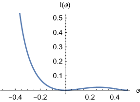
Figure 6: $I(\vartheta)$ as a function of $\vartheta$.

Appendix B Formula of butterfly velocity and charge diffusion constant

In this appendix we derive the formulas of $v_{B}$ and $D_{c}$, closely following the strategy presented in Roberts:2016wdl ; Blake:2016wvh ; Roberts:2014isa . Given a black hole metric in $d+2$ dimensions with the form

$$ds^{2}=-E(r)dt^{2}+B(r)dr^{2}+C(r)d\textbf{x}^{2},$$ (71)

whose components are expanded near the horizon $r_{h}$ as

$$E(r)\sim E^{\prime}(r_{h})(r-r_{h})+\cdots,\quad B(r)\sim B^{(-1)}(r_{h})(r-r_{h})^{-1}+\cdots,\quad C(r)\sim C(r_{h})+C^{\prime}(r_{h})(r-r_{h})+\cdots,$$ (72)

where $E^{\prime}(r_{h}),B^{(-1)}(r_{h}),C^{\prime}(r_{h})$ are finite and negative. We consider flat horizon and require that the asymptotic boundary is located at $r\to 0$. Then the black hole temperature and entropy density are

$$\begin{split}T&=\frac{1}{\beta}=\frac{-E^{\prime}(r_{h})}{4\pi\sqrt{B(r_{h})E(r_{h})}}=\frac{1}{4\pi}\sqrt{\frac{E^{\prime}(r_{h})}{B^{(-1)}(r_{h})}},\\ s&=\frac{C(r_{h})^{d/2}}{4G_{N}}.\end{split}$$ (73)

Chaos bound (2) is saturated in Einstein gravity. So

$$\lambda_{L}=2\pi T.$$ (74)

We are going to derive the butterfly velocity $v_{B}$ in terms of horizon quantities. Firstly we introduce the tortoise coordinate

$$dr_{*}=-\sqrt{\frac{B(r)}{E(r)}}dr$$ (75)

to write the metric into

$$ds^{2}=E(r)(-dt^{2}+dr_{*}^{2})+C(r)d\textbf{x}^{2},$$ (76)

where the asymptotic boundary is located at $r_{*}=0$ and the horizon is located at $r_{*}=-\infty$. Then we use the Kruskal coordinates

$$uv=-e^{4\pi r_{*}/\beta},\quad u/v=-e^{-4\pi t/\beta},$$ (77)

to further give

$$ds^{2}=2P(uv)dudv+Q(uv)d\textbf{x}^{2},$$ (78)

where $P(uv)=E(r)\frac{2}{uv}\left(\frac{\beta}{4\pi}\right)^{2},\,Q(uv)=C(r)$. The horizon is located at $uv=0$ and the asymptotic boundary is located at $uv=-1$. One can find

$$uv\sim(r-r_{h})\theta+\cdots,$$ (79)

where $\theta>0$. Applying the expression of $v_{B}$ in Roberts:2016wdl , we can obtain

$$v_{B}^{2}=\left(\frac{4\pi}{\beta}\right)^{2}\frac{P(0)}{2dQ^{\prime}(0)}=\frac{E^{\prime}(r_{h})}{dC^{\prime}(r_{h})},$$ (80)

where $P(0)=\frac{2E^{\prime}(r_{h})}{\theta}\left(\frac{\beta}{4\pi}\right)^{2}$ and $Q^{\prime}(0)=\frac{C^{\prime}(r_{h})}{\theta}$ have been used.

We add the Maxwell term ${\cal S}_{c}$ (30) into the action to study the charge diffusion. Following the method in Blake:2016wvh , we firstly write down the DC conductivity $\sigma$ and the susceptibility $\chi^{-1}$

$$\sigma=C(r_{h})^{\frac{d}{2}-1},\quad\chi^{-1}=\int_{0}^{r_{h}}C(r)^{-\frac{d}{2}}\sqrt{B(r)E(r)}dr.$$ (81)

Then the charge diffusion constant $D_{c}$ can be read from the Einstein relation

$$D_{c}=\frac{\sigma}{\chi}=C(r_{h})^{\frac{d}{2}-1}\int_{0}^{r_{h}}C(r)^{-\frac{d}{2}}\sqrt{B(r)E(r)}dr.$$ (82)

If above integration diverges, one can regularize it by introducing a UV cutoff $\Lambda_{\text{UV}}$ into the integral as $\int_{\Lambda_{\text{UV}}^{-1}}^{r_{h}}$.

Appendix C Numerical solutions for AdS-Schwarzschild black hole

Here we work on spatial dimension $d=2$. To study the $AdS_{4}-AdS_{4}$ domain wall, we choose the potential as

$$V(\phi)=-6-\phi^{2}+\frac{1}{8}\phi^{4}.$$ (83)

We adopt the domain wall ansatz

$$ds^{2}={\cal F}(r)^{-1}dr^{2}+e^{2{\cal A}(r)}(-{\cal F}(r)dt^{2}+dx_{1}^{2}+dx_{2}^{2}),\quad\phi=\phi(r).$$ (84)

The potential (83) allows three $AdS_{4}$ fixed points. One of them has the larger radius of AdS and stays in the UV ($r\to+\infty$), which is

$${\cal A}=r/L_{\text{UV}},\quad{\cal F}=1,\quad\phi=0$$ (85)

with scalar modes

$$\phi=\phi_{-}^{\text{UV}}e^{\Delta_{-}{\cal A}}+\phi_{+}^{\text{UV}}e^{\Delta_{+}{\cal A}},$$ (86)

where $L_{\text{UV}}=1,\Delta_{-}=1,\Delta_{+}=2$. The other two have the smaller radius of AdS and stay in the IR ($r\to-\infty$), one of which is

$${\cal A}=r/L_{\text{IR}},\quad{\cal F}=1,\quad\phi=\phi_{\text{IR}}$$ (87)

with scalar modes

$$\phi=\phi_{\text{IR}}+\phi_{-}^{\text{IR}}e^{\delta_{-}{\cal A}}+\phi_{+}^{\text{IR}}e^{\delta_{+}{\cal A}},$$ (88)

where $L_{\text{IR}}=\frac{\sqrt{3}}{2},\phi_{\text{IR}}=2,\delta_{\pm}=\frac{1}{2}(3\pm\sqrt{21})$. The other IR fixed point is obtained by the reflection $\phi\to-\phi$.

Firstly, we study the zero temperature flow. Given a slight deviation from the IR fixed point, the irrelevant IR modes $\phi_{-}^{\text{IR}}$ will be stimulated and intergraded to the UV fixed point. We find a UV-IR relation

$$(\phi_{-}^{\text{IR}})^{1/\delta_{-}}=Z_{\phi}(\phi_{-}^{\text{UV}})^{1/\Delta_{-}},$$ (89)

where the coefficient $Z_{\phi}=0.178$, which can be understood as a renormalization of operator $\cal O_{\phi}$.

Secondly, we study the thermal flow. Notice that three sorts of symmetries are contained in (84): the first is $r\to r+c$, which allows us to set the horizon at $r=0$; the second is $r\to rc,t\to t/c,{\cal F}\to{\cal F}c^{2}$, which allows us to set ${\cal F}^{\prime}(0)=1$; the third is $t\to tc^{2},x\to xc^{2},{\cal A}\to{\cal A}-\log c$, which allows us to set ${\cal A}(0)=0$. Then, under the last boundary condition which sets the value of $\phi(0)$, we can integrate the flow from the horizon to the UV. Be cautious that ${\cal F}(+\infty)$ is no longer equal to $1$ because of the gauge ${\cal F}^{\prime}(0)=1$. One should recover ${\cal F}(+\infty)=1$ by using the second symmetry inversely.

Finally, according to (73), (80) and (82), we can numerically determine the temperature $T$, butterfly velocity $v_{B}$ and diffusion ratios $D_{c}\lambda_{L}/v_{B}^{2}$ by using

$$T=\frac{e^{{\cal A}(0)}{\cal F}^{\prime}(0)}{4\pi},\quad v_{B}^{2}=\frac{{\cal F}^{\prime}(0)}{4{\cal A}^{\prime}(0)},\quad\frac{D_{c}\lambda_{L}}{v_{B}^{2}}=2e^{{\cal A}(0)}{\cal A}^{\prime}(0)\int_{0}^{\infty}e^{-{\cal A}(r)}\,dr.$$ (90)

Let us employ the standard quantization and consider the single trace deformation $W(\cal O_{\phi})=\cal O_{\phi}$. Considering the UV fixed point with relevant deformation, we can identify $\kappa_{s}=\phi_{-}^{\text{UV}}$ in (25), whose value can be extracted by $\phi=\phi_{-}^{\text{UV}}e^{\Delta_{-}\cal A}+\cdots$ in the UV. Considering the IR fixed point with irrelevant deformation, we can identify $\kappa_{s}=\phi_{-}^{\text{IR}}$ in (25), whose value is given by (89).

As $\Delta_{-}=1$, $T/\phi_{-}^{\text{UV}}$ is a dimensionless parameter. In the left plot of Figure 7, we plot the numerical result of the quantity $1-\frac{4}{3}v_{B}^{2}$ as a function of $T/\phi_{-}^{\text{UV}}$. The analytical results based on (25) for the UV fixed point and the IR fixed point are shown as well, where the constant $\gamma$ of the UV (IR) fixed point is calculated by using $\Delta_{-}$ ($\delta_{-}$). The numerical result matches well with the analytical results in both the $T\gg\phi_{-}^{\text{UV}}$ region and $T\ll\phi_{-}^{\text{UV}}$ region. The value of $v_{B}^{2}$ is also plotted in the phase diagram in Figure 1. When $\phi(0)\approx\phi_{\text{IR}}/2=1$, the effects of thermodynamic and $\cal O_{\phi}$ deformation are commensurate. At this time, $T/\phi_{-}^{\text{UV}}\approx 0.1$ can be understood as the vague boundary between the quantum critical region and the gapless low temperature phase.

In the right plot of Figure 7, we plot the numerical result of the quantity $\frac{D_{c}\lambda_{L}}{2v_{B}^{2}}-1$. The analytical result based on (31) for the UV fixed point is shown as well, where the constant $\eta$ is calculated by using $\Delta_{-}$. Note that the quantity $\frac{D_{c}\lambda_{L}}{2v_{B}^{2}}-1$ at low $T/\phi_{-}^{\text{UV}}$ behaves as $T/\phi_{-}^{\text{UV}}$ rather than $(T/\phi_{-}^{\text{UV}})^{-2\delta_{-}}$, which may result from the breakdown of (63), because the variation of the metric becomes divergent near asymptotic boundary of the IR region under an irrelevant deformation.

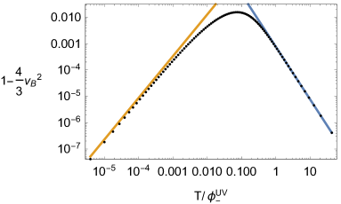
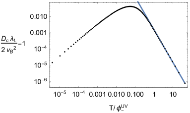
Figure 7: Quantities $1-\frac{4}{3}v_{B}^{2}$ and $\frac{D_{c}\lambda_{L}}{2v_{B}^{2}}-1$ as functions of $T/\phi_{-}^{\text{UV}}$. Points are results of numerical calculation and lines are results of perturbation analysis.

Appendix D Numerical solutions for Lifshitz black hole

For numerical calculation, we adopt the following ansatz

$$\begin{split}ds^{2}&=\frac{L^{2}}{r^{2}}\left(-\frac{(1-r)U(r)}{r^{2z-2}}e^{-S(r)}dt^{2}+\frac{dr^{2}}{(1-r)U(r)}+d\textbf{x}^{2}\right),\\ {\cal B}&=L\sqrt{\frac{2(z-1)}{z}}r^{-z}{\cal B}(r)(1-r)U(r)dt,\quad\phi=r^{\Delta_{-}}\phi(r),\end{split}$$ (91)

and choose the parameters in the action (36) as

$$W=\frac{dz}{L^{2}},\quad V(\phi)=-\frac{z^{2}+z(d-1)+d^{2}}{L^{2}}+\frac{\Delta_{-}(\Delta_{-}-(d+z))}{2L^{2}}\phi^{2}.$$ (92)

Then $L$ will not appear in the equation of motions. The asymptotic boundary is located at $r\to 0$ and the horizon is located at $r=1$. The boundary conditions at $r=0$ are $U(0)=1,S(0)=0,{\cal B}(0)=1,\phi(0)=\phi_{-}$, which ensure the asymptotic Lifshitz solution (37) with asymptotic behavior (21). The boundary conditions at $r=1$ are regular conditions.

According to (73) and (80), temperature $T$ and butterfly velocity $v_{B}$ in above ansatz are separately given by

$$T=\frac{U(1)}{4\pi}e^{-\frac{S(1)}{2}},\quad v_{B}^{2}=\frac{1}{2d}e^{-S(1)}U(1).$$ (93)

Firstly, we build up a Lifshitz black hole without scalar deformation by setting $\phi=0$. Then we calculate $\Phi(0)$ by evaluating $v_{B}^{2}/T^{2-\frac{2}{z}}$, whose values, as a function of $z$ in different spatial dimensions $d$, are shown in the left plot of Figure 2.

Secondly, we deform the Lifshitz black hole with scalar field. The value of $\Delta_{-}$ should satisfy $0<\Delta_{-}<\frac{d+z}{2}$ to make the deformation relevant. Then we can impose a small perturbation with non-zero $\phi_{-}$ and study the variation of $v_{B}$. The numerical results match (38) when $\phi_{-}\ll T^{\frac{\Delta_{-}}{z}}$, where the coefficient $\gamma$ as a function of $z$ for different $\Delta_{-}$ is shown in the right plot of Figure 2.

Appendix E Testing the relation between $v_{\text{th}}$ and $v_{\text{E}}$

We consider a neutral black hole with flat horizon and scalar hair. In Feng:2017wvc , the authors propose a relation between the thermodynamical volume density $v_{\text{th}}$ and the Euclidean bounded volume density $v_{\text{E}}$ as

$$v_{\text{th}}\doteq\sqrt{\frac{g_{1}}{h_{1}}}v_{\text{E}},$$ (94)

where $g_{1}$ and $h_{1}$ appear in the near horizon expansion of the black hole metric and the equality with a dot “$\doteq$” marks their supposition. In a $\rho$ coordinate, the metric appears as

$$ds^{2}=-h(\rho)dt^{2}+\frac{d\rho^{2}}{g(\rho)}+\frac{\rho^{2}}{L^{2}}d\textbf{x}^{2}$$ (95)

with the horizon expansion

$$h(\rho)\sim h_{1}(\rho-\rho_{h})+h_{2}(\rho-\rho_{h})^{2}+\cdots,\quad g(\rho)\sim g_{1}(\rho-\rho_{h})+g_{2}(\rho-\rho_{h})^{2}+\cdots$$ (96)

and the asymptotic boundary expansion

$$h(\rho)\sim\frac{\rho^{2}}{L^{2}}(1+\cdots-\frac{16\pi G_{N}m_{\text{BH}}L^{d+2}}{d\rho^{d+1}}+\cdots),\quad g(\rho)\sim\frac{\rho^{2}}{L^{2}}(1+\cdots+\frac{\#}{\rho^{d+1}}+\cdots).$$ (97)

The horizon is located at $\rho_{h}$ and the asymptotic boundary at $\rho\to\infty$. $m_{\text{BH}}$ is the mass density of the black hole. The Euclidean bounded volume density $v_{\text{E}}$ is

$$v_{E}=\frac{1}{d+1}\rho_{h}^{d+1}L^{-d}.$$ (98)

The thermodynamical volume density $v_{\text{th}}$ is determined by the general first law of black hole thermodynamics Kastor:2009wy ; Cvetic:2010jb

$$dm_{\text{BH}}=Tds+v_{\text{th}}dP,$$ (99)

where the thermodynamical pressure of the black hole is

$$P=\frac{d(d+1)}{16\pi G_{N}L^{2}}.$$ (100)

For a neutral black hole with flat horizon and scalar hair, there are two Smarr relations Feng:2017wvc

$$\begin{split}m_{\text{BH}}&=\frac{d}{d+1}Ts,\\ m_{\text{BH}}&=\frac{d}{d-1}Ts-\frac{4}{d-1}v_{\text{th}}P,\end{split}$$ (101)

which give

$$v_{\text{th}}P=\frac{1}{2}m_{\text{BH}}=\frac{d}{2(d+1)}Ts.$$ (102)

The hypothesis (94) relates the butterfly velocity $v_{B}$ to $v_{\text{th}}$ by

$$v_{B}^{2}=\sqrt{\frac{h_{1}}{g_{1}}}\frac{Ts}{4v_{\text{E}}P}\doteq\frac{Ts}{4v_{\text{th}}P}=\frac{d+1}{2d},$$ (103)

which leads to a constant $v_{B}$ and is in conflict with our analytical result in (23) and numerical result in Appendix C where the scalar hair is considered. Such contradiction results from the violation of hypothesis (94) .

Taking the coordinate transformation $\rho^{2}/L^{2}=C(\zeta)$, we can change (50) into (95) and check the hypothesis in (94). The result is

$$\sqrt{\frac{g_{1}}{h_{1}}}\frac{v_{\text{E}}}{v_{\text{th}}}=1-\frac{d+1}{2d}\lambda^{2}(I_{1}(1;\vartheta)+2I_{2}(1;\vartheta)),$$ (104)

where (53), (61) and (63) have been used. In general, the last term does not vanish. Especially, for $0<\vartheta<\frac{1}{2}$, it is non-positive. If further demanding one of the null-energy conditions, $T^{\rho}{}_{\rho}-T^{t}{}_{t}\geq 0$, we will have the inequality $\frac{g_{1}}{h_{1}}\geq 1$ and finally obtain

$$v_{\text{th}}\geq\sqrt{\frac{g_{1}}{h_{1}}}v_{\text{E}}\geq v_{\text{E}}$$ (105)

up to $O(\lambda^{2})$, which is the reverse isoperimetric inequality Feng:2017wvc .

References

- (1) D. Forster, “Hydrodynamic fluctuations, broken symmetry, and correlation functions”, in Reading, Mass., WA Benjamin, Inc.(Frontiers in Physics. Volume 47), 1975. 343 p., vol. 47, 1975.
- (2) Y. Sekino and L. Susskind, “Fast Scramblers,” JHEP 0810, 065 (2008) [arXiv:0808.2096 [hep-th]].
- (3) P. Hosur, X. L. Qi, D. A. Roberts and B. Yoshida, “Chaos in quantum channels,” JHEP 1602, 004 (2016) [arXiv:1511.04021 [hep-th]].
- (4) S. H. Shenker and D. Stanford, “Black holes and the butterfly effect,” JHEP 1403, 067 (2014) [arXiv:1306.0622 [hep-th]].
- (5) N. Sircar, J. Sonnenschein and W. Tangarife, “Extending the scope of holographic mutual information and chaotic behavior,” JHEP 1605, 091 (2016) [arXiv:1602.07307 [hep-th]].
- (6) R. G. Cai, X. X. Zeng and H. Q. Zhang, “Influence of inhomogeneities on holographic mutual information and butterfly effect,” arXiv:1704.03989 [hep-th].
- (7) J. Maldacena, S. H. Shenker and D. Stanford, “A bound on chaos,” JHEP 1608, 106 (2016) [arXiv:1503.01409 [hep-th]].
- (8) S. H. Shenker and D. Stanford, “Multiple Shocks,” JHEP 1412, 046 (2014) [arXiv:1312.3296 [hep-th]].
- (9) D. A. Roberts, D. Stanford and L. Susskind, “Localized shocks,” JHEP 1503, 051 (2015) [arXiv:1409.8180 [hep-th]].
- (10) A. Kitaev, “Hidden correlations in the hawking radiation and thermal noise,” (2014), talk given at the Fundamental Physics Prize Symposium, Nov. 10, 2014.
- (11) D. A. Roberts and D. Stanford, “Two-dimensional conformal field theory and the butterfly effect,” Phys. Rev. Lett. 115, no. 13, 131603 (2015) [arXiv:1412.5123 [hep-th]].
- (12) D. Stanford, “Many-body chaos at weak coupling,” JHEP 1610, 009 (2016) [arXiv:1512.07687 [hep-th]].
- (13) J. Polchinski and V. Rosenhaus, “The Spectrum in the Sachdev-Ye-Kitaev Model,” JHEP 1604, 001 (2016) [arXiv:1601.06768 [hep-th]].
- (14) D. A. Roberts and B. Swingle, “Lieb-Robinson Bound and the Butterfly Effect in Quantum Field Theories,” Phys. Rev. Lett. 117, no. 9, 091602 (2016) [arXiv:1603.09298 [hep-th]].
- (15) J. Maldacena and D. Stanford, “Remarks on the Sachdev-Ye-Kitaev model,” Phys. Rev. D 94, no. 10, 106002 (2016) [arXiv:1604.07818 [hep-th]].
- (16) P. Kovtun, D. T. Son and A. O. Starinets, “Viscosity in strongly interacting quantum field theories from black hole physics,” Phys. Rev. Lett. 94, 111601 (2005) [hep-th/0405231].
- (17) B. Swingle, G. Bentsen, M. Schleier-Smith and P. Hayden, “Measuring the scrambling of quantum information,” Phys. Rev. A 94, no. 4, 040302 (2016) [arXiv:1602.06271 [quant-ph]].
- (18) S. A. Hartnoll, “Theory of universal incoherent metallic transport,” Nature Phys. 11, 54 (2015) [arXiv:1405.3651 [cond-mat.str-el]].
- (19) M. Blake, “Universal Charge Diffusion and the Butterfly Effect in Holographic Theories,” Phys. Rev. Lett. 117, no. 9, 091601 (2016) [arXiv:1603.08510 [hep-th]].
- (20) M. Blake, “Universal Diffusion in Incoherent Black Holes,” Phys. Rev. D 94, no. 8, 086014 (2016) [arXiv:1604.01754 [hep-th]].
- (21) A. Lucas and J. Steinberg, “Charge diffusion and the butterfly effect in striped holographic matter,” JHEP 1610, 143 (2016) [arXiv:1608.03286 [hep-th]].
- (22) A. A. Patel and S. Sachdev, “Quantum chaos on a critical Fermi surface,” Proc. Nat. Acad. Sci. 114, 1844 (2017) [arXiv:1611.00003 [cond-mat.str-el]].
- (23) M. Blake and A. Donos, “Diffusion and Chaos from near AdS2 horizons,” JHEP 1702, 013 (2017) [arXiv:1611.09380 [hep-th]].
- (24) M. Baggioli, B. Goutéraux, E. Kiritsis and W. J. Li, “Higher derivative corrections to incoherent metallic transport in holography,” JHEP 1703, 170 (2017) [arXiv:1612.05500 [hep-th]].
- (25) K. Y. Kim and C. Niu, “Diffusion and Butterfly Velocity at Finite Density,” arXiv:1704.00947 [hep-th].
- (26) M. Baggioli and W. J. Li, “Diffusivities bounds and chaos in holographic Horndeski theories,” arXiv:1705.01766 [hep-th].
- (27) M. Blake, R. A. Davison and S. Sachdev, “Thermal diffusivity and chaos in metals without quasiparticles,” arXiv:1705.07896 [hep-th].
- (28) T. Hartman, S. A. Hartnoll and R. Mahajan, “An upper bound on transport,” arXiv:1706.00019 [hep-th].
- (29) Y. Gu, X. L. Qi and D. Stanford, “Local criticality, diffusion and chaos in generalized Sachdev-Ye-Kitaev models,” JHEP 1705, 125 (2017) [arXiv:1609.07832 [hep-th]].
- (30) R. A. Davison, W. Fu, A. Georges, Y. Gu, K. Jensen and S. Sachdev, “Thermoelectric transport in disordered metals without quasiparticles: The Sachdev-Ye-Kitaev models and holography,” Phys. Rev. B 95, no. 15, 155131 (2017) [arXiv:1612.00849 [cond-mat.str-el]].
- (31) Y. Gu, A. Lucas and X. L. Qi, “Energy diffusion and the butterfly effect in inhomogeneous Sachdev-Ye-Kitaev chains,” SciPost Phys. 2, 018 (2017) [arXiv:1702.08462 [hep-th]].
- (32) H. Shen, P. Zhang, R. Fan and H. Zhai, “Out-of-Time-Order Correlation at a Quantum Phase Transition,” arXiv:1608.02438 [cond-mat.str-el].
- (33) A. Bohrdt, C. B. Mendl, M. Endres and M. Knap, “Scrambling and thermalization in a diffusive quantum many-body system,” New J. Phys. 19, no. 6, 063001 (2017) [arXiv:1612.02434 [cond-mat.quant-gas]].
- (34) D. Chowdhury and B. Swingle, “Onset of many-body chaos in the model,” arXiv:1703.02545 [cond-mat.str-el].
- (35) S. Sachdev, “Quantum Phase Transitions,” 2nd Edition, Cambridge University Press (2011).
- (36) S. A. Hartnoll, “Lectures on holographic methods for condensed matter physics,” Class. Quant. Grav. 26, 224002 (2009) [arXiv:0903.3246 [hep-th]].
- (37) S. Sachdev, “Condensed Matter and AdS/CFT,” Lect. Notes Phys. 828, 273 (2011) [arXiv:1002.2947 [hep-th]].
- (38) S. A. Hartnoll, A. Lucas and S. Sachdev, “Holographic quantum matter,” arXiv:1612.07324 [hep-th].
- (39) A. Lucas, T. Sierens and W. Witczak-Krempa, “Quantum critical response: from conformal perturbation theory to holography,” arXiv:1704.05461 [hep-th].
- (40) J. Zaanen, “Superconductivity: Why the temperature is high,” Nature 430 (2004) 512.
- (41) X. Dong, S. Harrison, S. Kachru, G. Torroba and H. Wang, “Aspects of holography for theories with hyperscaling violation,” JHEP 1206, 041 (2012) [arXiv:1201.1905 [hep-th]].
- (42) B. Goutéraux and E. Kiritsis, “Generalized Holographic Quantum Criticality at Finite Density,” JHEP 1112, 036 (2011) [arXiv:1107.2116 [hep-th]].
- (43) B. Goutéraux, J. Smolic, M. Smolic, K. Skenderis and M. Taylor, “Holography for Einstein-Maxwell-dilaton theories from generalized dimensional reduction,” JHEP 1201, 089 (2012) [arXiv:1110.2320 [hep-th]].
- (44) J. McGreevy, “Holographic duality with a view toward many-body physics,” Adv. High Energy Phys. 2010, 723105 (2010) [arXiv:0909.0518 [hep-th]].
- (45) Y. Ling, P. Liu and J. P. Wu, “Holographic Butterfly Effect at Quantum Critical Points,” arXiv:1610.02669 [hep-th].
- (46) X. H. Feng and H. Lu, “Butterfly Velocity Bound and Reverse Isoperimetric Inequality,” Phys. Rev. D 95, no. 6, 066001 (2017) [arXiv:1701.05204 [hep-th]].
- (47) E. Witten, “Multitrace operators, boundary conditions, and AdS / CFT correspondence,” hep-th/0112258.
- (48) S. S. Gubser and I. Mitra, “Double trace operators and one loop vacuum energy in AdS / CFT,” Phys. Rev. D 67, 064018 (2003) [hep-th/0210093].
- (49) T. Faulkner, G. T. Horowitz and M. M. Roberts, “Holographic quantum criticality from multi-trace deformations,” JHEP 1104, 051 (2011) [arXiv:1008.1581 [hep-th]].
- (50) T. Faulkner, G. T. Horowitz and M. M. Roberts, “New stability results for Einstein scalar gravity,” Class. Quant. Grav. 27, 205007 (2010) [arXiv:1006.2387 [hep-th]].
- (51) Y. Ling, P. Liu and J. P. Wu, “Note on the butterfly effect in holographic superconductor models,” arXiv:1610.07146 [hep-th].
- (52) S. S. Gubser and A. Nellore, “Ground states of holographic superconductors,” Phys. Rev. D 80, 105007 (2009) [arXiv:0908.1972 [hep-th]].
- (53) M. M. Caldarelli, A. Christodoulou, I. Papadimitriou and K. Skenderis, “Phases of planar AdS black holes with axionic charge,” JHEP 1704, 001 (2017) [arXiv:1612.07214 [hep-th]].
- (54) S. Kachru, X. Liu and M. Mulligan, “Gravity duals of Lifshitz-like fixed points,” Phys. Rev. D 78, 106005 (2008) [arXiv:0808.1725 [hep-th]].
- (55) M. Taylor, “Non-relativistic holography,” arXiv:0812.0530 [hep-th].
- (56) M. Taylor, “Lifshitz holography,” Class. Quant. Grav. 33, no. 3, 033001 (2016) [arXiv:1512.03554 [hep-th]].
- (57) S. Sachdev and M. Mueller, “Quantum criticality and black holes,” J. Phys. Condens. Matter 21, 164216 (2009) [arXiv:0810.3005 [cond-mat.str-el]].
- (58) C. Charmousis, B. Goutéraux, B. S. Kim, E. Kiritsis and R. Meyer, “Effective Holographic Theories for low-temperature condensed matter systems,” JHEP 1011, 151 (2010) [arXiv:1005.4690 [hep-th]].
- (59) B. Goutéraux and E. Kiritsis, “Quantum critical lines in holographic phases with (un)broken symmetry,” JHEP 1304, 053 (2013) [arXiv:1212.2625 [hep-th]].
- (60) E. Kiritsis and J. Ren, “On Holographic Insulators and Supersolids,” JHEP 1509, 168 (2015) [arXiv:1503.03481 [hep-th]].
- (61) H. Liu and M. Mezei, “Probing renormalization group flows using entanglement entropy,” JHEP 1401, 098 (2014) [arXiv:1309.6935 [hep-th]].
- (62) U. Gursoy, E. Kiritsis, L. Mazzanti and F. Nitti, “Holography and Thermodynamics of 5D Dilaton-gravity,” JHEP 0905, 033 (2009) [arXiv:0812.0792 [hep-th]].
- (63) Y. Ling, Z. Y. Xian and Z. Zhou, “Holographic Shear Viscosity in Hyperscaling Violating Theories without Translational Invariance,” JHEP 1611, 007 (2016) [arXiv:1605.03879 [hep-th]].
- (64) K. Skenderis, “Lecture notes on holographic renormalization,” Class. Quant. Grav. 19, 5849 (2002) [hep-th/0209067].
- (65) A. Anabalon, D. Astefanesei, D. Choque and C. Martinez, “Trace Anomaly and Counterterms in Designer Gravity,” JHEP 1603, 117 (2016) [arXiv:1511.08759 [hep-th]].
- (66) D. Astefanesei, N. Banerjee and S. Dutta, “(Un)attractor black holes in higher derivative AdS gravity,” JHEP 0811, 070 (2008) [arXiv:0806.1334 [hep-th]].
- (67) D. B. Kaplan, J. W. Lee, D. T. Son and M. A. Stephanov, “Conformality Lost,” Phys. Rev. D 80, 125005 (2009) [arXiv:0905.4752 [hep-th]].
- (68) N. Iqbal, H. Liu, M. Mezei and Q. Si, “Quantum phase transitions in holographic models of magnetism and superconductors,” Phys. Rev. D 82, 045002 (2010) [arXiv:1003.0010 [hep-th]].
- (69) K. Jensen, A. Karch, D. T. Son and E. G. Thompson, “Holographic Berezinskii-Kosterlitz-Thouless Transitions,” Phys. Rev. Lett. 105, 041601 (2010) [arXiv:1002.3159 [hep-th]].
- (70) N. Iqbal, H. Liu and M. Mezei, “Lectures on holographic non-Fermi liquids and quantum phase transitions,” arXiv:1110.3814 [hep-th].
- (71) N. Evans, A. Gebauer, K. Y. Kim and M. Magou, “Phase diagram of the D3/D5 system in a magnetic field and a BKT transition,” Phys. Lett. B 698, 91 (2011) [arXiv:1003.2694 [hep-th]].
- (72) N. Iqbal, H. Liu and M. Mezei, “Quantum phase transitions in semilocal quantum liquids,” Phys. Rev. D 91, no. 2, 025024 (2015) [arXiv:1108.0425 [hep-th]].
- (73) K. Jensen, “More Holographic Berezinskii-Kosterlitz-Thouless Transitions,” Phys. Rev. D 82, 046005 (2010) [arXiv:1006.3066 [hep-th]].
- (74) D. Z. Freedman, S. S. Gubser, K. Pilch and N. P. Warner, “Renormalization group flows from holography supersymmetry and a c theorem,” Adv. Theor. Math. Phys. 3, 363 (1999) [hep-th/9904017].
- (75) D. Kastor, S. Ray and J. Traschen, “Enthalpy and the Mechanics of AdS Black Holes,” Class. Quant. Grav. 26, 195011 (2009) [arXiv:0904.2765 [hep-th]].
- (76) M. Cvetic, G. W. Gibbons, D. Kubiznak and C. N. Pope, “Black Hole Enthalpy and an Entropy Inequality for the Thermodynamic Volume,” Phys. Rev. D 84, 024037 (2011) [arXiv:1012.2888 [hep-th]].
- (77) M. M. Qaemmaqami, “On the Butterfly Effect in 3D Gravity,” arXiv:1707.00509 [hep-th].
- (78) M. Alishahiha, A. Davody, A. Naseh and S. F. Taghavi, “On Butterfly effect in Higher Derivative Gravities,” JHEP 1611, 032 (2016) [arXiv:1610.02890 [hep-th]].
- (79) M. M. Qaemmaqami, “Criticality in Third Order Lovelock Gravity and Butterfly effect,” arXiv:1705.05235 [hep-th].