Universal scaling relation for magnetic sails: momentum braking in the limit of dilute interstellar media

Abstract

The recent progress in laser propulsion research has advanced substantially the prospects to realize interstellar spaceflight within a few decades. Here we examine passive deceleration via momentum braking from ionized interstellar media. The very large area to mass relations needed as a consequence of the low interstellar densities, of the order of 0.1 particles per $\mathrm{cm}^{3}$, or lower, are potentially realizable with magnetic sails generated by superconducting coils. Integrating the equations of motion for interstellar protons hitting a Biot Savart loop we evaluate the effective reflection area $A(v)$ in terms of the velocity $v$ of the craft. We find that the numerical data is fitted over two orders of magnitude by the scaling relation $A(v)\ =\ 0.081A_{R}\log^{3}(I/(\beta I_{c}))$, where $A_{R}=\pi R^{2}$ is the bare sail area, $I$ the current and $\beta=v/c$. The critical current $I_{c}$ is $1.55\cdot 10^{6}$ Ampere. The resulting universal deceleration profile can be evaluated analytically and mission parameters optimized for a minimal craft mass.

For the case of a sample high speed transit to Proxima Centauri we find that magnetic momentum braking would involve daunting mass requirements of the order of $10^{3}$ tons. A low speed mission to the Trappist-1 system could be realized on the other side already with a 1.5 ton spacecraft, which would be furthermore compatible with the specifications of currently envisioned directed energy launch systems. The extended cruising times of the order of $10^{4}$ years imply however that a mission to the Trappist-1 system would be viable only for mission concepts for which time constrains are not relevant.

• May 2017

Keywords: magnetic sail, Biot Savart loop, interstellar spaceflight, momentum braking

1 Introduction

Research in interstellar travel technologies has seen a paradigm change over the last few years. Early concept studies, like the Orion [1] and the Daedalus [2] project, envisioned gigantic fusion based starships [3]. The perspective changed however when efforts to develop miniaturized satellites, i.e. waferSats [4], were expanded to designs of spacecraft-on-the-chip probes suitable for deep space exploration [5]. The low weight of these nanocrafts would allow to accelerate them at launch to a substantial fraction of the speed of light by ground- or space based arrays of lasers disposing of an overall power of the order of 100 GW [5]. Other aspects of long-duration interstellar missions, such as the feasibility of self-healing electronics based on silicon nanowire gate-all-around FET [6] and the interaction of relativistic spacecrafts with the interstellar medium [7], have also been addressed.

The ever longer list of known exoplanets [8] includes by now nearby potentially habitable planets [9, 10]. The number of promising interstellar mission concepts is likewise increasing, ranging presently from high speed Proxima Centauri flybys [11] to slow cruising Genesis missions aiming to establish autonomously developing biospheres of unicellular organisms on transiently habitable exoplanets [12]. These developments warrants hence to reexamine the options available to decelerate the interstellar probe passively on arrival.

Spacecrafts travel essentially unimpeded through the voids of deep space, which is characterized by very low particle densities. Electromagnetic fields produced by the craft may however reach far enough for the spacecraft to transfer its kinetic momentum slowly to the interstellar medium. One speaks of a magnetic sail [13], as illustrated in Fig. 1, for the case that a magnetic field produced by a superconducting Biot Savart loop does the job of reflecting the $H^{+}$ ions of the interstellar medium.

The requirements for a magnetic sail are daunting. Firstly, because currents of typically $10^{6}$ Ampere are needed to generate a magnetic field capable to reflect protons at relativistic speeds, and secondly due to the low particle density of typically less than one particle per cm³ of the interstellar medium. Performing numerical simulations valid in the limit of low interstellar particle densities we show here that a single universal scaling function describes the dynamics of magnetic sails to an astonishing accuracy. The resulting model, which can be evaluated analytically, may hence serve as a reference model. We also point out that previous estimates [13] for the operational properties of magnetic sails have been rather on the optimistic side.

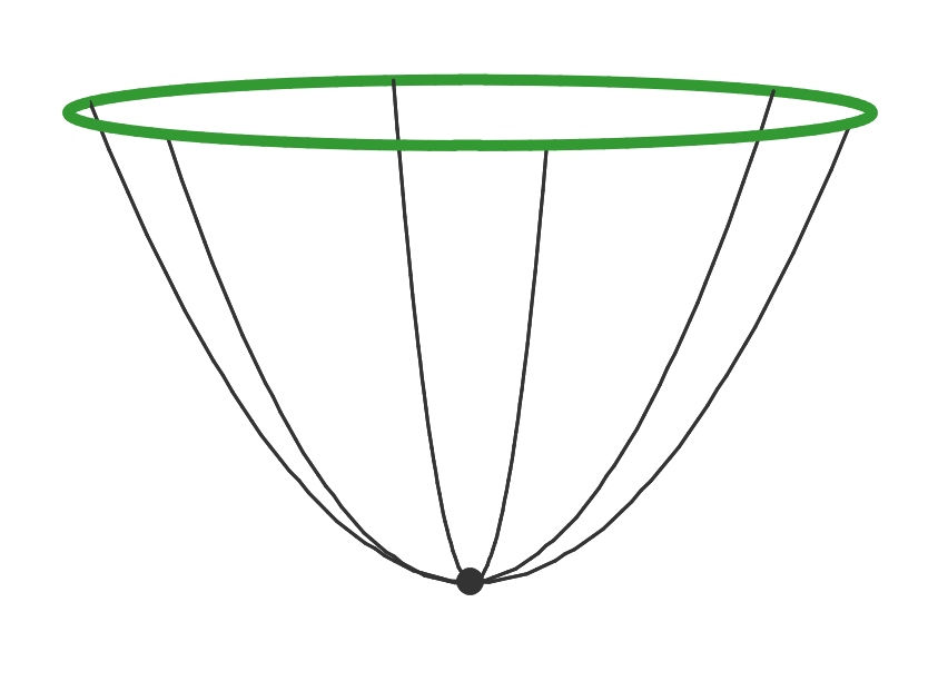
Figure 1: Illustration of a magnetic sail in the form of a superconducting Biot Savart loop (green). Forces are transmitted via tethers (black lines) to the payload (filled sphere) located in front of the sail.

2 Passive interstellar deceleration

Passive deceleration techniques of interstellar crafts are based on transferring the momentum of the probe to other media. The three options for braking are to transfer momentum to either the

• interstellar medium,

• the stellar wind of the target star or

• to the photons of the target star.

For the last possibility a photon sail is used [14, 15], just in the reverse modus operandi [16]. For the first two options momentum is transferred to charged particles, with the difference being that the particle density of stellar winds is somewhat higher than that of the interstellar space. Passive deceleration of interstellar crafts is both suitable and necessary for interstellar missions for which the overall duration is irrelevant [12], such as missions aiming to offer life alternative evolutionary pathways [17, 18, 19].

2.1 Interstellar medium

The interstellar neighborhood of the sun is characterized to a distance of about 15 lightyears by a collection of interstellar clouds, with the local interstellar cloud interacting with the G cloud. Together they are embedded into the local bubble, which reaches out to roughly 300 lightyears [20].

Interstellar clouds vary strongly in their properties. Typical densities of ionized hydrogen are of the order of $n_{p}=0.05-0.20$ cm^-3 for the warm local clouds [20] and about 0.005 cm^-3 for the voids of the local bubble [21]. Patches of isolated cold interstellar clouds with less than 200 AU (astronomical units) in diameter may have on the other hand large densities of neutral hydrogen, up to the order of 3000 cm^-3 [22].

Passive deceleration of an interstellar probe based on transferring kinetic energy to ionized hydrogen, i.e. to protons, is hence substantially more difficult for destinations located in the local bubble. We investigate this problem here in the limit of independent particles, touching shortly on the possible formation of magnetic bow shocks in Appendix B.

2.2 Impulse braking

An interstellar craft with a total mass $m_{tot}$ and an area $A$ perpendicular to the cruising direction encounters $Avn_{p}$ particles per second, where $n_{p}=f_{ISM}\cdot 10^{6}$ m^-3 is the density of protons and $v=v(t)$ the velocity. The factor $f_{ISM}$ characterizes the interstellar medium, with $f_{ISM}\approx 0.1/0.005$ for the local cloud and respectively the local bubble.

Impulse braking takes place when the particles encountered are reflected. The velocity of the craft then changes as

$$\frac{d}{dt}\Big{(}m_{tot}v\Big{)}\ =\ -\big{(}A(v)n_{p}v\big{)}\,\big{(}2m_{p}v\big{)}$$ (1)

for the case that the incoming particles of mass $m_{p}$ are fully reflected. Here we investigate how the effective reflection area $A=A(v)$ depends on the velocity $v$ of the craft for the case that the interstellar protons are reflected by the magnetic field of a current carrying loop. Alternatively one may consider the reflection of interstellar ions from electric sails [23, 24].

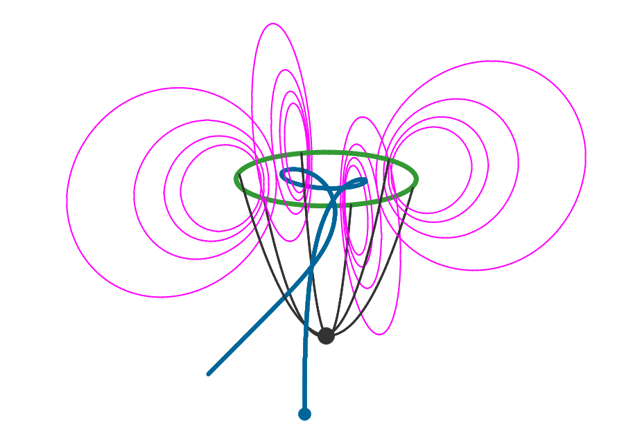
Figure 2: A proton with mass $m_{p}$ (blue curve), starting with $v=0.01\,\mathrm{c}$ with an initial offset $r=0.88\,R$ from the center (blue dot), is partly reflected by the magnetic field (pink lines) of a Biot Savart loop (green circle), carrying in turn a current of $I=10^{5}$ A. The process is scale invariant with respect to the radius $R$ of the loop. The normalized scalar product $\mathbf{v}_{i}\cdot\mathbf{v}_{f}/v^{2}$ between the initial and the final velocities, $\mathbf{v}_{i}$ and respectively $\mathbf{v}_{f}$, is here $\mathbf{v}_{i}\cdot\mathbf{v}_{f}/v^{2}=-0.61$. The direction of flight of the spacecraft is in this perspective from top to down.

2.3 Biot Savart magnetic sail

Charged particles may be partially reflected by the magnetic field

$$\mathbf{B}(\mathbf{x})\ =\ \frac{\mu_{0}I}{4\pi}\int_{L}\frac{d\mathbf{l}^{\prime}\times(\mathbf{x}-\mathbf{x}^{\prime})}{|\mathbf{x}-\mathbf{x}^{\prime}|^{3}}$$ (2)

of a current carrying loop $L$, as illustrated in Fig. 2. For a loop of radius $R$ the field strength $B_{0}=B(0)$ at the center is

$$B_{0}\ =\ \frac{\mu_{0}I}{2R}~{}.$$ (3)

As a reference we remark that $B_{0}=2\pi\cdot 10^{-7}$ Tesla for $R=1$ m and a current of $I=1$ Ampere. After testing for accuracy we have used for our numerical simulations 12-48 segments as subdivisions for the Biot Savart loop. The trajectories, such as the one shown in Fig. 2, have then been evaluated by a straightforward numerical integration of the non-relativistic Lorentz force

$$m_{p}\dot{\mathbf{v}}\ =\ q\,\mathbf{v}\times\mathbf{B}~{},$$ (4)

where $m_{p}$ and $q$ are respectively the proton mass and charge.

A particle in a homogeneous field $B$ performs circular orbits for which the radius, the Larmor radius $r_{L}$, is

$$r_{L}\ =\ \frac{mv}{|q|B}\ =\frac{2m_{p}v}{|q|\mu_{0}I}\,R~{},$$ (5)

where we assumed in the second step that $B=B_{0}$, as given by (3). For the case of protons the Larmor radius (in meters) is given by $3.13\,\beta/B[\mathrm{Tesla}]$.

A magnetic sail functions when the Larmor radius remains within the craft diameter, viz when $r_{L}<2R$. With $\beta=v/c$ the expression (5) for the Larmor radius then implies that

$$I\ >\ \frac{m_{p}c}{|q|\mu_{0}}\,\beta\ \approx\ \beta\cdot 2.5\cdot 10^{6}\,\mathrm{Ampere}$$ (6)

needs to be fulfilled, as an order of magnitude estimate, if protons are to be reflected by the magnetic field of the loop. We note that the radius $R$ does not enter (6).

3 Scaling of the effective reflection area

We consider here the axial configuration, i.e. that the center magnetic field is aligned with the initial velocity $\mathbf{v}_{i}$ of the particles. Integrating the trajectories of protons arriving at a distance $r$ from the center of the Biot Savart loop we did evaluate the normalized scalar product between the initial and the final velocities, $\mathbf{v}_{i}$ and $\mathbf{v}_{f}$ respectively,

$$S(r)\ =\ {\bf v}_{i}\cdot{\bf v}_{f}/v^{2},\qquad|{\bf v}_{i}|=v=|{\bf v}_{f}|~{}.$$

The particle is unaffected by the magnetic sail for $S(r)=1$ and fully reflected for $S(r)=-1$.

Selected results for $S(r)$ are presented in Fig. 3. The alignment of the direction of the velocity with the magnetic field at the center of the loop results in a central hole, corresponding to $S(r)\to 1$. It is evident that $S(r)$ is otherwise strongly non-monotonic, with perfect transmission $S(r)\to 1$ being recovered again with increasing distance $r$. The data presented in Fig. 3 is fully scale invariant with respect to the loop radius $R$, as we have confirmed numerically.

The effective reflection area $A(v)$ can be obtained in a second step by integrating $S(r)$ over all distances $r$ from the center of the Biot Savart loop:

$$A(v)\ =\ 2\pi\int_{0}^{\infty}\frac{1-S(r)}{2}\,rdr~{}.$$ (7)

The data can be fitted, as evident from the results presented in Fig. 4, to a surprising accuracy by the log-polynomial scaling function

$$A(v)\ =\ A_{c}\left[\log\left(\frac{I}{\beta I_{c}}\right)\right]^{3},\qquad v<(cI)/I_{c}~{},$$ (8)

where $\beta=v/c$ is the relativistic velocity, $I$ the current through the wire and $A_{c}=0.081\,\pi R^{2}$. The area enclosed by the Biot Savart loop is $\pi R^{2}$.

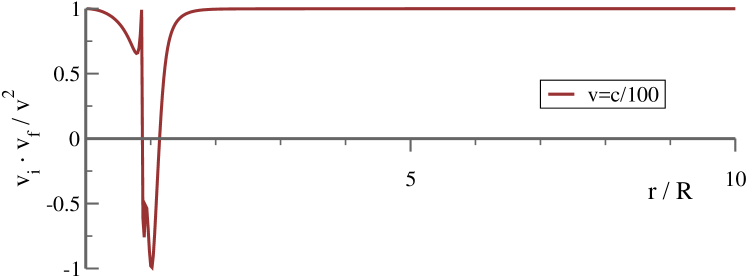
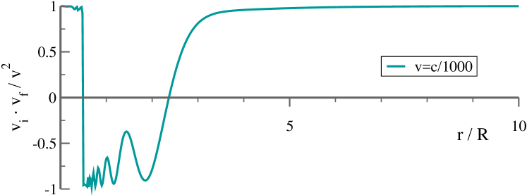
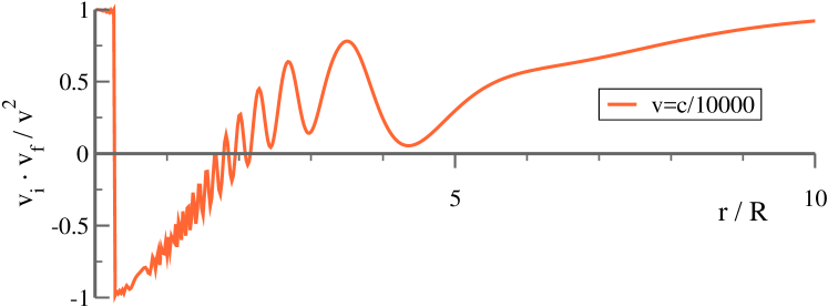
Figure 3: The normalized scalar product $\mathbf{v}_{i}\cdot\mathbf{v}_{f}/v^{2}$ between the the initial and the final velocities, $\mathbf{v}_{i}$ and respectively $\mathbf{v}_{f}$, of a proton hitting a Biot Savart loop with a current of $10^{5}$ Ampere at a distance $r$ from the center. The velocity of the proton is $c/100$, $c/1000$ and $c/10000$ from top to bottom. The magnetic field at the center is along the $z$-axis and hence parallel to $\mathbf{v}_{i}$. Note the highly non-monotonic features and that the magnetic sail becomes ineffective for $v>cI/I_{c}=c/15.5=0.065c$, see (8). The normalized scalar product $\mathbf{v}_{i}\cdot\mathbf{v}_{f}/v^{2}$ is a function of only $r/R$ and hence fully scale invariant with respect to the loop radius $R$.

The effective reflection area $A(v)$ vanishes altogether when $I<\beta\,I_{c}$  Ampere, where the numerical result (8) for the critical current, $I_{c}=1.55\cdot 10^{6}$  Ampere, reflects the order of magnitude estimate (6). We note that we cannot resolve numerically whether $A(v)$ really vanishes for $v>cI/I_{c}$, or if it drops to finite but exceedingly small values.

• The data presented in Fig. 4 for $I=10^{5}$ Ampere scales with $v/I$, as we have verified numerically. This scaling, which has been included in (8), results from the linear scaling of the Lorenz force with the magnetic field $B$, which increases in turn linearly with the current $I$. The radius $R$ of the Biot-Savat loop only enters as a prefactor.

• The functional form of the scaling relations (8) cannot be traced back, to our knowledge, to underlying physical arguments. It is however interesting to point out that a powerlaw scaling [13] such as $A_{V}\sim(v/c)^{\alpha}$, would be inconsistent with the existence of a critical current $I_{c}$. The log-argument $\log(I/(\beta I_{c})$ in (8) captures on the other hand the fact that the effective reflection area $A_{v}$ vanishes for $v/c>I/I_{c}$.

• In an equivalent study of magnetic sails in the axial configuration, Andrews and Zubrin [25] found $A(v)\approx 75$ for $R=100$ km, $B_{0}=10^{-5}$ Tesla and $v=750$ km/s, corresponding to $I=1.6\cdot 10^{6}$ Ampere and $v=c/400$ respectively. Using identical parameters we find with $A(v)=18$, a substantially more conservative estimate. We also note that Andrews and Zubrin [25] proposed scaling relations which are inconsistent with the here presented results. The source for these discrepancies are unclear.

We note that the effective reflection area $A(v)$ coincides with the loop area when $A(v)=\pi R^{2}$, viz when $I/\beta=15.6\cdot 10^{6}\,\mathrm{Ampere}$ .

3.1 Universal deceleration profile

Substituting $A(v)$ from (8) into the equation of motion (1) for the craft we find

$$\frac{\dot{v}/v}{\log^{3}(vI_{c}/(cI))}\ =\ \frac{2m_{p}n_{p}A_{c}}{m_{tot}}\,v~{},$$ (9)

which can be solved for $v=v(x)$ as

$$\frac{1}{\log^{2}(vI_{c}/(cI))} = \frac{1}{\log^{2}(v_{0}I_{c}/(cI))}$$ (10)

$$+ \frac{4m_{p}n_{p}A_{c}}{m_{tot}}\,(x_{0}-x)~{},$$

where $v_{0}=v(x_{0})$ is the initial velocity. In the following we set $x_{0}=0$. The speed drops to zero at a distance $x_{max}$, which can be expressed as

$$x_{max}\ =\ \frac{1/0.081}{\log^{2}(v_{0}I_{c}/(cI))}\,\frac{1}{4m_{p}n_{p}}\,\frac{m_{tot}}{\pi R^{2}}~{}.$$ (11)

Here we have used that $A_{c}=0.081\pi R^{2}$. The stopping distance $x_{max}$ may be used to write the determining equation (10) for the velocity as

$$v=v_{0}\,e^{a}\exp\left(\frac{-a}{\sqrt{1-x/x_{max}}}\right),\quad x\in[0,x_{max}]\,,$$ (12)

where $a=\log(cI/(v_{0}I_{c}))>0$. Reversing (12) one find

$$\frac{x}{x_{max}}\ =\ 1-\frac{a^{2}}{(\log(v/v_{0})-a)^{2}}~{}.$$ (13)

The speed profile (12) determines via $dt=dx/v$ also the time

$$t\ =\ \frac{e^{-a}}{v_{0}}\int_{0}^{x}dx^{\prime}\exp\left(a/\sqrt{1-x^{\prime}/x_{max}}\right)$$ (14)

needed to cruise a given distance $x$. Note that $a>0$ and that (14) hence diverges for $x\to x_{max}$.

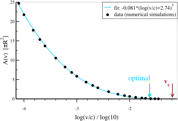
Figure 4: The effective reflection area $A(v)$ of the magnetic sail, see (7), as obtained by simulating numerically the trajectories of protons hitting a Biot Savart loop (black bullets). The current is $I=10^{5}$ Ampere. The effective area $A(v)$ is given in units of the bare loop area $\pi R^{2}$ and the velocity as $\log(v/c)$, to base ten. The fit of the data using (8) (blue line) is excellent when optimizing the two parameters $A_{c}$ and $I_{c}$. The brown and blue arrows indicate respectively the critical $v_{c}=c/15.5$ entering (8) and the velocity $c/42$ corresponding to the optimal current (16).

3.2 Optimal current

A straightforward route to optimize mission profiles is to minimize the stopping distance (11) for a given total mass $m_{tot}$. We assume here that $m_{tot}$ is dominated by the mass of the magnetic sail, which is in turn proportional to $IR$. We need hence to minimize

$$\frac{z^{2}}{\log^{2}(z)},\qquad z=\frac{I}{\beta_{0}I_{c}}$$ (15)

as a function of $z$. The minimum of (15), $\log(z)=1$, $z=e\approx 2.71$, determines then the current

$$I_{opt}\ =\ \beta_{0}\cdot 4.2\cdot 10^{6}\,\mathrm{Ampere}$$ (16)

minimizing the stopping distance $x_{max}$ for a given total mass $m_{tot}$. The resulting effective reflection area (8) is

$$A(v)\ =\ A_{c}\left[1+\log(v_{0}/v)\right]^{3},\qquad I=I_{opt}~{},$$ (17)

where we have used that $\log(ev_{0}/v)=1+\log(v_{0}/v)$. Deceleration starts therefore with a very small effective area, viz with $A(v_{0})/(\pi R^{2})=0.081$.

Using the optimality condition (16), that is

$$a\ =\ \log(z)\big{|}_{z=e}\ =\ 1~{},$$ (18)

one may evaluate the deceleration profile for a given deceleration ratio $v/v_{0}$.

• From (13) we find that $v/v_{0}=1/10$ is reached at $x=0.91\,x_{max}$. For the time the craft needs to decelerate one then obtains, when integrating (14) numerically, $t=1.84\,x_{max}/v_{0}$.

• After a cruising time of $5.2\,x_{max}/v_{0}$ the craft arrives later on at $x=0.98\,x_{max}$, at which point its speed is reduced to $v_{0}/300$.

Note that $x_{max}/v_{0}$ is the time the craft would need to cover the stopping distance $x_{max}$ at its nominal speed $v_{0}$.

4 Sample mission profiles

In the following we use the optimal current (16), for which $a=\log(I/(\beta_{0}I_{c}))=1$. The stopping distance (11) may be written consequently as

$$x_{max}\ =\ \frac{3.1}{m_{p}n_{p}}\,\frac{m_{tot}}{\pi R^{2}}~{}.$$ (19)

In the next step we determine suitable $x_{max}$ from a time balancing principle.

4.1 Balancing cruising and deceleration

We consider here mission profiles for which the time $t_{cruise}$ and $t_{stop}$ the craft spends respectively for cruising and for deceleration are the same order of magnitude. For a 2:1 ratio we have that $t_{cruise}=2\,t_{stop}$. The overall time to arrive to the destination is $t_{cruise}+t_{stop}$.

For concreteness we consider two distinct sample missions.

• A high speed mission to Proxima Centauri with $\beta_{0}=1/10$. The distance $D$ to destination is $4.2$ lyr.

• A slow speed mission to Trappist-1 characterized by $v_{0}=c/300=1000$ km/s and $D=39.5$ lyr [26].

We demand in both cases that the insertion velocity is $c/3000=100$ km/s. The final velocity reduction to planetary velocities is in this scenario assumed to be performed by braking from stellar wind protons or photons. We need hence velocity reduction factors $v/v_{0}$ of 1/300 for the PC mission and of 1/10 for T1. We use further that the respective deceleration distances $x$ are close to the stopping distance, i.e. that $x\approx x_{max}$, as discussed in Sect. 3.2. The balancing of the cruising and the deceleration time then determines $x_{max}$ via

$$t_{cruise}=2\,t_{stop},\qquad\frac{D-x_{max}}{v_{0}}=2\,\tau(v/v_{0})\frac{x_{max}}{v_{0}}~{},$$

where $\tau(1/10)=1.84$ and $\tau(1/300)=5.2$. The stopping distance is then

$$x_{max}=\frac{D}{1+2\tau(v/v_{0})}\ =\ \left\{\begin{array}[]{rl}0.37\,\mathrm{lyr}&\mathrm{PC}\\ 8.44\,\mathrm{lyr}&\mathrm{T1}\end{array}\right.$$ (20)

for the Proxima Centauri and respectively for the Trappist-1 mission. The total traveling times are $58$ year for PC and 12000 years for T1.

4.2 Mass requirements

The mass $m_{MS}$ of the magnetic sail is

$$m_{MS}=2\pi R\,\frac{I\rho_{I}}{10^{6}}~{},$$ (21)

where $\rho_{I}$ is the mass density per meter of a wire supporting $10^{6}$ Ampere. We will use in the following $\rho_{I}=0.18$ kg/m, which is, as discussed in Appendix A, a value one can reach with state of the art high temperature superconducting tapes.

For the total mass $m_{tot}$ of the spacecraft, including tethers and payload, we assume here that it is roughly the double of the mass $m_{MS}$ of the magnetic sail. Using (16), (19) and (21) we then find

$$R=\ 0.6\cdot 10^{3}\,\frac{\beta_{0}}{f_{ISM}\,x_{max}[\mathrm{lyr}]}$$ (22)

for the radius $R$ of the magnetic sail (in km). For the PC and the T1 mission respectively we have $f_{ISM}=0.1/0.005$ and hence

$$R\ =\ \left\{\begin{array}[]{rl}1600\,\mathrm{km}&\mathrm{PC}\\ 47\,\mathrm{km}&\mathrm{T1}\end{array}\right.$$ (23)

and respectively $m_{tot}=1500$ tons for PC and $m_{tot}=1.5$ tons for T1. To decelerate fast interstellar spacecrafts is exceedingly demanding. Above results show however also that it is possible to transfer the kinetic energy of slow cruising probes to the interstellar medium even when it is rarefied as within the local bubble. The craft parameters, $v_{0}=c/300$ and $m_{tot}=1.5$ tons, would fit furthermore the specifications of currently envisioned directed energy launch systems [27].

Slow cruising interstellar probes would need of the order of $10^{4}$ years to return data, which is clearly not a viable option for a science mission. The possibility to explicitly optimize the performance of the sail, i.e. the effective reflection area (8), has allowed us on the other hand to show that interstellar missions not limited by time constraints [12] are feasible. Passive deceleration using magnetic sails is in this case possible with low-mass crafts.

4.3 Constant time trajectories

Instead of balancing the times needed to cruise and to decelerate one may also consider mission profiles characterized by a given total travelling time $T_{D}=t_{cruise}+t_{stop}$. The stopping distance is then given by

$$x_{max}\ =\ \frac{v_{0}T_{D}-D}{\tau(v/v_{0})-1}~{}.$$ (24)

For a $T_{D}=100$ years transit to Proxima Centauri we $x_{max}=1.4$ lyr, $R=430$ km and $m_{tot}=400$ tons. The improvement with respect to (23) is about a factor four.

5 Maneuvering in stellar winds

The velocity $v_{SW}$ of the solar wind is $v_{SW}\sim(400-750$) km/s for equatorial winds in the ecliptic and polar winds respectively [28]. Both the velocity and the density $n_{SW}$ of the solar wind depend strongly on the state of the sun in terms of the sunspot cycle. As a function of the distance $r$ from the star the particle density $n_{SW}=n_{SW}(r)$ of a stellar wind falls off like

$$n_{SW}=n_{AU}\frac{r_{AU}^{2}}{r^{2}},\qquad n_{AU}\approx(1-10)\left[\frac{1}{\mathrm{cm}^{3}}\right],$$ (25)

where AU stands for astronomical unit.

Magnetic braking using the stellar wind is only possible when the luminosity of the central star is dim enough that it does not heat up the superconducting material. This is the case in the outskirts of M dwarfs systems, for which modeling efforts [29] indicate that both the wind velocity and the proton density $n_{AU}$ at 1 AU distance increase with a decreasing mass of the star. For conservative estimates of the wind properties of M dwarfs one may hence use solar system parameters.

The temperature $T$ of a passively cooling craft is given by the per surface area balance

$$2\sigma T^{4}\ =\ \frac{L}{L_{\Sun}}\left(\frac{R_{AU}}{r}\right)^{2}W_{\Sun}$$ (26)

between twice the emitted black body and the absorbed stellar radiation. $W_{\Sun}=1400\,\mathrm{W}/\mathrm{m}^{2}$ is here the solar constant, $L$ and $L_{\Sun}$ the luminosity of the target star and the sun respectively and $\sigma=5.67\cdot 10^{-8}\,\mathrm{W}\mathrm{m}^{-2}\mathrm{K}^{-4}$ the Stefan Boltzmann constant. For a conservative estimate we have assumed that the reflectivity vanishes.

An operating temperature of $T=30$ K is reached for a craft in the Trappist-1 system, for which $L=0.00052L_{\Sun}$ [26], when $R>2.8R_{AU}$. A superconducting material with a critical temperature of $T=90$ K would allow to operate the magnetic sail even further in, albeit only when reducing correspondingly the current $I$, down to $R=0.3R_{AU}$.

5.1 Stellar wind pressure vs. gravitational pull

Both the gravitational attraction

$$F_{G}=\frac{Gm_{tot}m_{S}}{r^{2}}$$ (27)

and the force

$$F_{SW}=2A(v+v_{SW})m_{p}(v+v_{SW})^{2}n_{AU}\frac{r_{AU}^{2}}{r^{2}}$$ (28)

the craft experience from reflecting the protons of the stellar wind decay with $1/r^{2}$. Note that the stellar wind velocity $v_{SW}$ adds in (28) to the relative velocity between the craft and the protons. For an estimate of magnitude of the $v=0$ ratio

$$\frac{F_{G}}{F_{SW}} = \frac{1}{2m_{p}v_{SW}^{2}n_{AU}}\,\frac{Gm_{S}}{r^{2}_{AU}}\,\frac{m_{tot}}{A(v_{SW})}$$

$$= \frac{1}{6.2v_{SW}^{2}}\,\frac{n_{p}}{n_{AU}}\,\frac{Gm_{S}}{r^{2}_{AU}}\,x_{max}\frac{\pi R^{2}}{A(v_{SW})}$$

between $F_{G}$ and $F_{SW}$ we use (19) and the solar system values $n_{AU}=5\,\mathrm{cm}^{-3}$ and $v_{SW}=500$ km/s [29]. One obtains

$$\frac{F_{G}}{F_{SW}}\ =\ 7\,f_{ISM}\,\frac{m_{S}}{m_{\Sun}}\,\frac{\pi R^{2}}{A(v_{SW})}\,x_{max}[\mathrm{lyr}]~{},$$ (29)

where the mass $m_{S}$ of the central star has been measured in terms of the solar mass $m_{\Sun}$. The condition (29) for the force balance is fulfilled for most magnetic sails tailored for interstellar braking. For the case of the T1 mission we obtain, when using $v_{0}/v_{SW}=2$, $m_{S}/m_{\Sun}\sim 0.1$ and (17), that $F_{G}\sim 0.08F_{SW}$. The craft may hence maneuver freely within the outskirts of the Trappist-1 system defined by the radiation balance (26).

6 Conclusions

Simulating the motion of individual particles in the magnetic field generated by a current carrying loop we found that the effective reflection area can be fitted to a surprising accuracy by a single scaling function. Our simulations accurately describe magnetic sails in the limit of low interstellar particle densities. The universal deceleration profile resulting from the log-polynomial scaling function found for the effective reflection area may hence be considered as a reference model for magnetic momentum braking.

Our results are valid for an idealized magnetic sail in the axial configuration. The study of additional effects like the influence of the thermal motion of the interstellar protons on the performance of the magnetic sail is also possible Preliminary simulations show in this respect that the effective reflection area remains unaffected at high velocities, shrinking however when thermal and craft velocities start to become comparable.

Magnetic sails fail to operate when the magnetic field generated by the current through the loop is too weak to transfer momentum to the interstellar protons. The technical feasibility of magnetic sails is hence dependent in first place on the availability of materials able to support elevated critical currents. Using the properties of state of the art $2^{\mathrm{nd}}$ generation high temperature superconducting tapes and otherwise conservative estimates for the mission parameters we find that magnetic sails need to be massive, in the range of $10^{3}$ tons, in order to be able to decelerate high speed interstellar crafts.

Optimizing the requirements for a trajectory to the Trappist-1 system we found importantly that magnetic braking is possible for low-speed crafts even when the target star is located within the local bubble, that is when the particle density of the interstellar medium is as low as 0.005 cm^-3. In this case a 1.5 ton craft could do the job. The launch requirements of such a craft would be furthermore compatible with the specifications [27] of the directed energy launch system envisioned by the Breakthrough Starshot project [11] for Centauri flybys, which could hence see dual use. The extended cruising time of the order $10^{4}$ years implies however that slow cruising trajectories are only an option for mission, such as for life-carrying Genesis crafts [12], not expected to yield near-term results in terms of a tangible scientific return.

Appendix A: Materials for superconducting wires

State of the art coated conductors for power applications are produced in the form of tapes, where a superconducting YBCO layer is sandwiched between a metallic substrate and a top cover [30]. Critical currents of the order of $(3-7)\cdot 10^{6}$ Ampere/cm² are routinely achieved [31]. These $2^{\mathrm{nd}}$ generation high temperature superconducting tapes would be suitable for magnetic sails.

• The overall mass requirements for superconducting tapes depends on the exact specification, like the material and the thickness used for the metallic substrate. Taking here the specific mass $8.9\,\mathrm{g}/\mathrm{cm}^{3}$ of copper as a reference, we find that a wire capable to support a current of $10^{6}$ Ampere would weight about $(8.9/5)$ g/cm length, which implies that $\rho_{I}=0.18$ kg/m. Compare (21).

• Envisioned operating temperatures of 30 Kelvin or lower [31] fit well with deep-space environments in which the superconducting wire would cool down passively via black body radiation.

• The metallic substrate of the superconducting sandwich is generically designed to take up a substantial amount of magnetomechnical stress. Additional supporting structures besides the tethers are hence not necessary.

The quality of the superconducting tapes is the key parameter determining overall mission requirements. The hard cutoff (6) determines directly the minimal current at which the sail stops working, with a reasonable working regime for the current being given by (16). For a given type of superconducting tape the mass per length necessary to support the field generating current is therefore dependent solely on the initial velocity $v_{0}$.

Appendix B: Magnetic bow shocks

The field of the Biot Savart loop on the axis, taken here as the z-axis, is

$$B(z)\ =\ \frac{\mu_{0}I}{2R}\,\frac{R^{3}}{\left(z^{2}+R^{2}\right)^{3/2}}\ \approx\ B_{0}\,\frac{R^{3}}{z^{3}}~{},$$ (30)

where we have taken the large $z$ limit in the second step. A bow shock occurs when a current carrying layer of charged particles forms upstream from the craft. The magnetic field generated by this current then compensates the magnetic field on the outside, doubling it however on the inner side. The position of the bow shock it determined in order of magnitude by the equilibrium between magnetic and kinetic pressures [13], respectively when the corresponding energy densities match:

$$n_{p}m_{p}\frac{v^{2}}{2}\ =\ \frac{(2B)^{2}}{2\mu_{0}}\ \approx\ \frac{2B_{0}^{2}}{\mu_{0}}\,\frac{R^{6}}{z^{6}}~{}.$$ (31)

This is clearly only a rough estimate. For the earth the surface field $B_{0}\approx 20\cdot 10^{6}$ Tesla interacts further out with the solar wind, for which $n_{p}\approx 5\,\mathrm{cm}^{-3}$ and $v\approx 450$ km/s. One finds that $z/R\approx 26$ whereas the the bow shock of the earth forms at around 15 radii.

6.1 Larmor radius at shock position

A bow shock can establish itself only if the magnetic field $B(z)$ is strong enough to deflect the protons within the dimensions of shock [32], i.e. when $r_{L}<z$. Using (5) for the Larmor radius $r_{L}=r_{L}(z)$ we hence need that

$$\frac{m_{p}v}{|q|2B(z)}<z,\qquad\frac{z^{2}}{R^{2}}<\frac{\mu_{0}qI}{m_{p}v}=\frac{\mu_{0}qI_{wr}}{m_{p}c}\frac{cI}{vI_{wr}}~{},$$ (32)

where we have taken $2B(z)$ as the inner magnetic field strength and the working-regime current $I_{wr}$ from (16). For the earth the Larmor radius of solar wind protons at the shock location $z=15\,R$ is with $\sim 24$ km much lower than the extension of the bow shock. Plugging in the numbers we find that the Larmor radius $r_{L}$ will be smaller than the extend $z$ of the bow shock if

$$z\ <\ 2.5\,R\left(\frac{cI}{vI_{wr}}\right)^{1/2}$$ (33)

holds. Note that $cI/(vI_{wr})=1$ at the boundary of the working regime.

6.2 Bow shock condition

We rewrite the expression (31) for the position of the bow shock with the help of (30) as

$$\frac{z^{6}}{R^{6}}=\frac{\mu_{0}I^{2}}{R^{2}n_{p}m_{p}v^{2}}=\frac{\mu_{0}I_{wr}^{2}}{R_{0}^{2}n_{p}m_{p}c^{2}}\,\frac{R_{0}^{2}}{R^{2}}\left(\frac{cI}{vI_{wr}}\right)^{2}~{},$$ (34)

where we have used $c$, $I_{wr}$ and $R_{0}=100$ km as scales. With these number we obtain

$$\frac{z}{R}\ =\ \frac{2.4}{\left(f_{ISM}\right)^{1/6}}\left(\frac{R_{0}}{R}\right)^{1/3}\left(\frac{cI}{vI_{wr}}\right)^{1/3}$$ (35)

for the distance $z$ of the bow shock from the craft.

Comparing with (33) we observe that the two conditions (35) and (33) are only marginally compatible. It is hence not clear to which extend a bow shock forms. Detailed investigations of the magnetosphere of the craft need therefore numerical methods which go beyond magneto hydrodynamics [32, 33].

A precondition for a bow shock to form is that the interstellar protons are deflected in the first case. Zubrin and Andrews proposed however, as based on a plasma fluid model for the bow shock, that a spacecraft characterized by $I=159\cdot 10^{3}$ Ampere and $v=c/10$ could be decelerated effectively by magnetic sails [13]. Our analysis, see (8), indicates in contrast that a craft with this kind of mission parameters would be right on the point where protons are not reflected at all, viz on the point where the effective reflection area $A(v\to v_{c})$ vanishes.

References

References

- [1] Freeman J Dyson. Discussion paper: Interstellar transport. Annals of the New York Academy of Sciences, 163(1):347–357, 1969.
- [2] Alan Bond and Anthony R Martin. Project daedalus. Journal of the British Interplanetary Society, 31:S5–S7, 1978.
- [3] KF Long. Project icarus: The first unmanned interstellar mission, robotic expansion & technological growth. Journal of the British Interplanetary Society, 64(4):107, 2011.
- [4] Travis Brashears, Philip Lubin, Nic Rupert, Eric Stanton, Amal Mehta, Patrick Knowles, and Gary B Hughes. Building the future of wafersat spacecraft for relativistic spacecraft. In SPIE Optical Engineering+ Applications, pages 998104–998104. International Society for Optics and Photonics, 2016.
- [5] Philip Lubin. A roadmap to interstellar flight. arXiv preprint arXiv:1604.01356, 2016.
- [6] Dong-Il Moon, Jun-Young Park, Jin-Woo Han, Gwang-Jae Jeon, Jee-Yeon Kim, John Moon, Myeong-Lok Seol, Choong Ki Kim, Hee Chul Lee, M Meyyappan, et al. Sustainable electronics for nano-spacecraft in deep space missions. In Electron Devices Meeting (IEDM), 2016 IEEE International, pages 31–8. IEEE, 2016.
- [7] Thiem Hoang, A Lazarian, Blakesley Burkhart, and Abraham Loeb. The interaction of relativistic spacecrafts with the interstellar medium. The Astrophysical Journal, 837(1):5, 2017.
- [8] Jean Schneider, Cyrill Dedieu, Pierre Le Sidaner, Renaud Savalle, and Ivan Zolotukhin. Defining and cataloging exoplanets: the exoplanet. eu database. Astronomy & Astrophysics, 532:A79, 2011.
- [9] Guillem Anglada-Escudé, Pedro J Amado, John Barnes, Zaira M Berdiñas, R Paul Butler, Gavin AL Coleman, Ignacio de La Cueva, Stefan Dreizler, Michael Endl, Benjamin Giesers, et al. A terrestrial planet candidate in a temperate orbit around proxima centauri. Nature, 536(7617):437–440, 2016.
- [10] Jason A Dittmann, Jonathan M Irwin, David Charbonneau, Xavier Bonfils, Nicola Astudillo-Defru, Raphaëlle D Haywood, Zachory K Berta-Thompson, Elisabeth R Newton, Joseph E Rodriguez, Jennifer G Winters, et al. A temperate rocky super-earth transiting a nearby cool star. Nature, 544(7650):333–336, 2017.
- [11] Zeeya Merali. Shooting for a star. Science, 352(6289):1040–1041, 2016.
- [12] Claudius Gros. Developing ecospheres on transiently habitable planets: the genesis project. Astrophysics and Space Science, 361(10):324, 2016.
- [13] Robert M Zubrin and Dana G Andrews. Magnetic sails and interplanetary travel. Journal of Spacecraft and Rockets, 28(2):197–203, 1991.
- [14] Malcolm Macdonald and Colin McInnes. Solar sail science mission applications and advancement. Advances in Space Research, 48(11):1702–1716, 2011.
- [15] Bo Fu, Evan Sperber, and Fidelis Eke. Solar sail technology—a state of the art review. Progress in Aerospace Sciences, 86:1–19, 2016.
- [16] René Heller and Michael Hippke. Deceleration of high-velocity interstellar photon sails into bound orbits at centauri. The Astrophysical Journal Letters, 835(2):L32, 2017.
- [17] Francis HC Crick and Leslie E Orgel. Directed panspermia. Icarus, 19(3):341–346, 1973.
- [18] M Meot-Ner and GL Matloff. Directed panspermia- a technical and ethical evaluation of seeding nearby solar systems. British Interplanetary Society, Journal(Interstellar Studies), 32:419–423, 1979.
- [19] Michael Noah Mautner. Directed panspermia. 3. strategies and motivations for seeding star-forming clouds. Journal of British Interplanetary Society, 50:93–102, 1997.
- [20] Priscilla C Frisch, Seth Redfield, and Jonathan D Slavin. The interstellar medium surrounding the sun. Annual Review of Astronomy and Astrophysics, 49:237–279, 2011.
- [21] Barry Y Welsh and Robin L Shelton. The trouble with the local bubble. Astrophysics and Space Science, 323(1):1–16, 2009.
- [22] David M Meyer, JT Lauroesch, JEG Peek, and Carl Heiles. The remarkable high pressure of the local leo cold cloud. The Astrophysical Journal, 752(2):119, 2012.
- [23] Pekka Janhunen. Electric sail for spacecraft propulsion. Journal of Propulsion and Power, 20(4):763–764, 2004.
- [24] Nikolaos Perakis and Andreas M Hein. Combining magnetic and electric sails for interstellar deceleration. Acta Astronautica, 128:13–20, 2016.
- [25] Dana G Andrews and Robert M Zubrin. Magnetic sails and interstellar travel. British Interplanetary Society, Journal, 43:265–272, 1990.
- [26] Michaël Gillon, Amaury HMJ Triaud, Brice-Olivier Demory, Emmanuël Jehin, Eric Agol, Katherine M Deck, Susan M Lederer, Julien De Wit, Artem Burdanov, James G Ingalls, et al. Seven temperate terrestrial planets around the nearby ultracool dwarf star trappist-1. Nature, 542(7642):456–460, 2017.
- [27] Travis Brashears, Philip Lubin, Gary B Hughes, Kyle McDonough, Sebastian Arias, Alex Lang, Caio Motta, Peter Meinhold, Payton Batliner, Janelle Griswold, et al. Directed energy interstellar propulsion of wafersats. In SPIE Optical Engineering+ Applications, pages 961609–961609. International Society for Optics and Photonics, 2015.
- [28] DJ McComas, HA Elliott, NA Schwadron, JT Gosling, RM Skoug, and BE Goldstein. The three-dimensional solar wind around solar maximum. Geophysical research letters, 30(10), 2003.
- [29] CP Johnstone, M Güdel, T Lüftinger, G Toth, and I Brott. Stellar winds on the main-sequence-i. wind model. Astronomy & Astrophysics, 577:A27, 2015.
- [30] Xavier Obradors and Teresa Puig. Coated conductors for power applications: materials challenges. Superconductor Science and Technology, 27(4):044003, 2014.
- [31] Maxime Leroux, Karen J Kihlstrom, Sigrid Holleis, Martin W Rupich, Srivatsan Sathyamurthy, Steven Fleshler, HP Sheng, Dean J Miller, Serena Eley, Leonardo Civale, et al. Rapid doubling of the critical current of yba2cu3o7- coated conductors for viable high-speed industrial processing. Applied Physics Letters, 107(19):192601, 2015.
- [32] Yasumasa Ashida, Ikkoh Funaki, Hiroshi Yamakawa, Hideyuki Usui, Yoshihiro Kajimura, and Hirotsugu Kojima. Two-dimensional particle-in-cell simulation of magnetic sails. Journal of Propulsion and Power, 30(1):233–245, 2013.
- [33] Ikkoh Funaki and Hiroshi Yamakawa. Research status of sail propulsion using the solar wind. J Plasma Fusion Res, 8:1580–4, 2009.