Delay Properties of Energy Efficient Ethernet Networks

Abstract

Networking operational costs and environmental concerns have lately driven the quest for energy efficient equipment. In wired networks, energy efficient Ethernet (EEE) interfaces can greatly reduce power demands when compared to regular Ethernet interfaces. Their power saving capabilities have been studied and modeled in many research articles in the last few years, together with their effects on traffic delay. However, to this date, all articles have considered them in isolation instead of as part of a network of EEE interfaces. In this paper we develop a model for the traffic delay on a network of EEE interfaces. We prove that, whatever the network topology, the per interface delay increment due to the power savings capabilities is bounded and, in most scenarios, negligible. This confirms that EEE interfaces can be used in all but the most delay constrained scenarios to save considerable amounts of power.

I Introduction

As part of the ongoing effort to reduce energy demands of networking infrastructure, energy efficient Ethernet (EEE) interfaces were first standardized in [1] for transmission speeds up to 10 Gb$/$s in copper medium, and later expanded to 40 and 100 Gb$/$s speeds in [2]. Their introduction has permitted significant energy usage reductions of up to 90% in low load periods with little additional delay. EEE interfaces of speeds up to 10 Gb$/$s have one low power idle (LPI) mode designed to save energy when there are no transmissions. Usually, an EEE interface transitions to this LPI mode when the transmission queue depletes. To minimize latency, the normal operating mode is restored as soon as a new frame is ready for transmission [3]. The transitions to the LPI mode and back take a non negligible amount of time (of the order of a single frame transmission) that increases latency and wastes some energy, as the energy needs are comparable to that of an active interface.

Several articles have studied and modeled the performance of EEE interfaces [4, 5, 3, 6]. However, to the best of our knowledge, all of them have considered the simplified case of an isolated switch. This article models the effects of a network of 10 Gb/s EEE interfaces on the traffic delay. We consider two representative network topologies that form the basis of more complex ones. In the first one, a single EEE interface aggregates the traffic coming from a group of Ethernet interfaces. The second one consists on a series of EEE interfaces. We have found that the aggregating interface behaves like an isolated EEE one, irrespective of whether the previous interfaces in the network have energy saving capabilities. In the second case, we demonstrate that the per interface added delay converges to a constant value. Finally, we prove that, in both cases, the penalty for deploying EEE interfaces, i.e. the delay increment per interface compared to regular Ethernet interfaces, is bounded.

II Traffic Aggregation

Figure 1: A group of interfaces sending traffic to an aggregating switch.

We first consider a two stage network like the one shown in Fig. 1. At the first stage, a group of interfaces send traffic to a single switch at the second stage. This second switch aggregates traffic to a single outgoing link via an EEE interface. We are interested in the delay suffered at this second stage.

There already exist several results in the literature for the delay model of an isolated energy efficient interface [4, 7, 8, 9]. However, most of them require the frame arrivals to form a Poisson (or Poisson-like) process. Unfortunately, the output of the interfaces in the first stage hardly ever follows a Poisson process. This only happens if the frame sizes follow an exponential distribution, the arrivals already followed a Poisson process at the first stage and the first stage interfaces have no vacations, i.e., they are not energy efficient themselves [10].

However, when we consider the aggregated output of the first stage as a whole, we can make use of the Palm–Khintchine theorem that states that this aggregate resembles a Poisson process when the number of independent contributors is large enough. We make use of this result, and of the average delay model for Poisson traffic in [4] ($\overline{W}_{\text{EEE}}$), to approximate the average delay at the second stage interface as

$$\overline{W}_{\text{agg}}\approx\overline{W}_{\text{EEE}}=\frac{1+\lambda^{2}\sigma_{S}^{2}}{2\lambda(1-\rho)}+\frac{1-\rho}{2\lambda}+\frac{(\lambda T_{\mathrm{W}})^{2}-2}{2\lambda(1+\lambda T_{\mathrm{W}})},$$ (1)

where $\lambda$ is the average incoming traffic rate, $\sigma_{S}^{2}$ is the transmission time variance, $\rho$ is the traffic load and $T_{\mathrm{W}}$ is the setup time of the interface.

However, the delay in (1) is not only caused by the energy saving algorithm. A significant part is due to regular traffic queuing. According to the Pollaczek-Khinchine formula, the queuing delay at a regular Ethernet interface receiving Poisson traffic can be calculated as

$$\overline{W}_{\text{M/G/1}}=\frac{\rho+\lambda\mu\sigma_{S}^{2}}{2(\mu-\lambda)},$$ (2)

with $\mu=1/\overline{S}$, and $\overline{S}$ denoting the average transmission time.

Therefore, the delay caused by the energy savings capabilities is clearly

$$\begin{split}\Delta\overline{W}_{\text{agg}}&=\overline{W}_{\text{agg}}-\overline{W}_{\text{M/G/1}}\\ &=\frac{1-\rho^{2}}{2\lambda(1-\rho)}+\frac{1-\rho}{2\lambda}+\frac{(\lambda T_{\mathrm{W}})^{2}-2}{2\lambda(1+\lambda T_{\mathrm{W}})},\end{split}$$ (3)

that after some straightforward algebra becomes

$$\Delta\overline{W}_{\text{agg}}=\frac{T_{\mathrm{W}}}{2}\left(1+\frac{1}{1+\lambda T_{\mathrm{W}}}\right).$$ (4)

Note that $T_{\mathrm{W}}/2\leq\Delta\overline{W}_{\text{agg}}\leq T_{\mathrm{W}}\,\,\forall\lambda\geq 0$ and that, at the same time, it does not have any dependence on the variance of the frame sizes and just depends on the average arrival rate.

III Interfaces in Tandem

Figure 2: A network with two interfaces in tandem.

We now consider a network composed of two network interfaces in tandem ($b^{0}$ and $b^{1}$) as depicted in Fig. 2. Again, we are interested in the waiting time at the second interface, as the delay at the first one has already been studied in the literature. Although it is infrequent to encounter in practice a series of network interfaces, it is a valid approximation to the case where a single incoming port of a switch represents the majority of the incoming traffic, even when the main contributor changes over time from one port to another.

For the analysis we will consider two different cases: one where the first interface is not energy efficient, i.e., it is a regular Ethernet interface, and a second one where both interfaces are energy efficient. In both cases we assume that all links have the same nominal capacity.

III-A A Regular Ethernet Interface Followed by an EEE Interface

We now consider the case of a regular Ethernet interface followed by an EEE interface. This system, when considered as a whole, can be directly modeled as a single EEE interface. The first interface shapes the traffic reaching the second interface as if it were a token bucket with generating rate equal to the outgoing link capacity. For constant size frames, it is easily seen that the interarrival times of the frames reaching the second interface are never shorter than the transmission time. Hence, any queue at the second interface must only be due to its energy saving algorithm, and must remain otherwise unaffected by the actual traffic load, as it is capped at the first interface. The average waiting time at the second interface in this case can be calculated subtracting the waiting time at a regular Ethernet interface ($\overline{W}_{\text{regular}}$) from the waiting time of an energy efficient interface ($\overline{W}_{\text{EEE}}$):

$$\overline{W}_{\text{tandem}}^{\text{regular}}=\overline{W}_{\text{EEE}}-\overline{W}_{\text{regular}}.$$ (5)

In the case where the arrivals at the first interface form a Poisson process, $\overline{W}_{\text{EEE}}=\overline{W}_{\text{agg}}$ from (1) and $\overline{W}_{\text{regular}}=\overline{W}_{\text{M/G/1}}$. So, it is clear that

$$\overline{W}_{\text{tandem}}^{\text{regular}}=\Delta\overline{W}_{\text{agg}}=\frac{T_{\mathrm{W}}}{2}\left(1+\frac{1}{1+\lambda T_{\mathrm{W}}}\right).$$ (6)

In this case, all the delay is due to the energy saving algorithm. Hence, as before, this delay is bounded by $T_{\mathrm{W}}$ and is only dependent on the average traffic rate.

III-B A Series of Interfaces in Tandem

A more interesting scenario is the one formed by two (or more) consecutive energy efficient interfaces. Although the result will be surprisingly simple, the model is a bit more elaborated than the previous one.

According to the status of the first interface ($b^{0}$), a new frame can arrive to it either while it is sleeping, transitioning to sleep, active or transitioning to active. We first consider the case where the first interface is either active or transitioning to active when a frame arrives. Let frame $i$ be the $i$-th frame to arrive at the interface in the current busy cycle, so it either arrives at $b^{0}$ while it is active or transitioning to active. Then, according to the Lindley’s recursion, its waiting time at the second interface $b^{1}$ is $W^{1}_{i}=W^{1}_{i-1}+s^{1}_{i-1}-x^{1}_{i}$, with $s^{j}_{i-1}$ being the service time of frame $i-1$ at interface $b^{j}$ and $x^{j}_{i}$ the interarrival time at $b^{j}$ between frames $i-1$ and $i$. However, it is clear that $x^{1}_{i}=s^{0}_{i}$, as the queue at $b^{0}$ was, by hypothesis, non empty when $i$ arrived at it. At the same time, $s^{0}_{i}=s^{1}_{i}$ as the capacity of both links attached to the interfaces is the same, so we must conclude that $W_{i}^{1}=W_{i-1}^{1}+s^{1}_{i-1}-s^{1}_{i}$. Finally, recall that frame 1 must have reached $b^{1}$ in the sleeping state, as it is the first one of the current busy cycle. In this case the interface immediately starts the transition to active, so $W^{1}_{1}=T_{\mathrm{W}}$. Therefore

$$W^{\text{green}}_{\text{tandem}}(i)=T_{\mathrm{W}}+s^{1}_{1}-s^{1}_{i}\leq T_{\mathrm{W}}+s^{1}_{i}\quad\forall i\geq 0,$$ (7)

when $b^{0}$ is active at frame $i$ arrival.

A frame can also reach $b^{0}$ when all the previous traffic has already departed. In this case, $b^{0}$ is either sleeping or transitioning to sleep. In either case, the frame must wait at $b^{0}$ to end the transition to sleep and then return to the active state after a time $T_{\mathrm{W}}$. When the frame finally reaches $b^{1}$ it must be in the sleeping state as any pending transition to sleep must have already concluded. So, the frame just waits at $b^{1}$ for a time $T_{\mathrm{W}}$ while it is transitioning to active. So

$$W^{\text{green}}_{\text{tandem}}(i)=T_{\mathrm{W}}\quad\forall i\geq 0,$$ (8)

when $b^{0}$ is sleeping at frame $i$ arrival.

It easily follows that if more energy efficient interfaces are added to the network in the same fashion, each one will add between $T_{\mathrm{W}}$ and $T_{\mathrm{W}}+S$ seconds of delay, with $S=\max_{i}\{s_{i}\}$. So, if we consider a series of $n$ energy efficient interfaces, the total delay would be included in

$$\overline{W}_{\text{first}}+(n-1)T_{\mathrm{W}}\leq\overline{W}_{\text{tandem}}\leq\overline{W}_{\text{first}}+(n-1)(T_{\mathrm{W}}+S),$$ (9)

where $\overline{W}_{\text{first}}$ is the average delay at the first green interface in the series. Recall that if the first green interface receives Poisson traffic, $\overline{W}_{\text{first}}=\overline{W}_{\text{EEE}}$. If, however, the first energy efficient interface is in tandem with a previous non energy efficient interface, $\overline{W}_{\text{first}}=\overline{W}_{\text{tandem}}^{\text{regular}}$.

We can now study the added delay cost due to the energy efficient operation in a series of tandem switches with identical capacity. We compare the delay of a series of regular Ethernet interfaces to that of a series of green interfaces. In the first case, assuming again Poisson arrivals, the total delay is just the queuing delay at the first interface, as the arrival rate at the rest is never greater than their output link capacity, plus the one due to the frame size differences at each successive link, so the total delay is bounded by $\overline{W}_{\textrm{M/G/1}}+(n-1)S$. In the energy efficient tandem, $\overline{W}_{\text{first}}=\overline{W}_{\text{EEE}}$, so the difference is

$$\begin{split}\Delta\overline{W}_{\text{tandem}}&=\overline{W}_{\text{EEE}}+(n-1)T_{\mathrm{W}}+(n-1)S\\ &-(\overline{W}_{\text{M/G/1}}+(n-1)S)\\ &=\overline{W}_{\text{tandem}}^{\text{regular}}+(n-1)T_{\mathrm{W}}\\ &=\frac{T_{\mathrm{W}}}{2}\left(2n+\frac{1}{1+\lambda T_{\mathrm{W}}}-1\right)\leq nT_{\mathrm{W}}.\end{split}$$ (10)

As expected, the per interface added delay converges to

$$\lim_{n\to\infty}\frac{\Delta\overline{W}_{\text{tandem}}}{n}=T_{\mathrm{W}}.$$ (11)

IV Experimental Validation

We have tested our models with the help of the ns-2 simulator [11]. To this end, we have employed an in-house developed module implementing the EEE frame transmission policy [12]. We chose popular 10GBASE-T interfaces, so the transition lengths to idle and to active are, respectively, $2.88\,\mu$s and $4.48\,\mu$s [1]. We have performed a series of experiments for each of the developed models both with synthetic traffic traces and real traffic from the CAIDA project [13]. Each experiment with synthetic traffic has been repeated ten times with different random seeds, and then we have obtained the 95% confidence interval of every measure. The synthetic traffic traces have been modeled with exponential and Pareto interarrival times, in the latter case with $\alpha=2.5$. In both cases frame sizes follow a bimodal distribution to approximate real Internet traffic [14]. We employed a frame size of 100 bytes with a 54% probability and a size of 1500 bytes with a 46% probability.

IV-A Results for the Traffic Aggregation Scenario

We first proceed with the case where many interfaces send traffic to an aggregator. The first state of the network consists on a varying number of interfaces (from 2 to 100), each receiving an independent traffic stream, although of equal average rate.

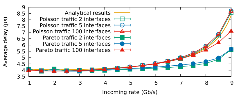
Figure 3: Delay at the second interface when receiving traffic from multiple independent non energy efficient interfaces.

Figure 3 shows the results for the case where only the second stage interface is energy efficient. As expected, for the scenario with 100 aggregators the results match the model with extraordinary accuracy. Also note that the results for the scenario with just two interfaces at the first stage exhibit an unexpected level of accuracy, and only the Pareto traffic shows little deviations from the theoretical values at the highest loads, where EEE is less useful, as its energy savings decay with load. Recall that the model is only valid for large values of contributors and that the output of each first stage link does not follow a Poisson distribution, since the frame sizes are not exponentially distributed. As the number of interfaces increases the results rapidly converge to the model prediction.

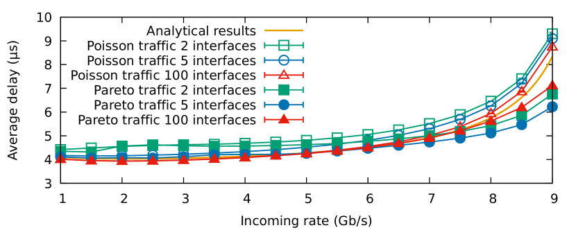
Figure 4: Delay at the second interface when receiving traffic from multiple independent energy efficient interfaces.

The results for the case where all the links have power saving capabilities is shown in Fig. 4. Again, the results for 100 first-stage interfaces match the model almost perfectly, as expected. However, in this case the results for the two interfaces case deviate some more from the model, because the energy saving algorithm adds additional correlation to the output of the interfaces. As before, results rapidly converge to the model if the number of interfaces increases, with the results for just five users showing a very good match. In all cases, the results are accurate enough to validate the model for any number of aggregating interfaces.

IV-B Results for the Tandem Network

This section shows the results for a network composed of two consecutive Ethernet interfaces.

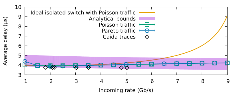
Figure 5: Delay at the second interface when receiving traffic from a single regular Ethernet interface.

The results for the non energy efficient interface followed by an EEE one are represented in Fig. 5. The delay experienced in the second interface always falls inside the bounds predicted by the model. Note that, contrary to what happened in the aggregating scenarios, the delay departs from that suffered by an isolated link. This is because there is no queuing delay at this second interface due to traffic load as the incoming traffic rate to this interface is never greater than its outgoing link capacity. It is also remarkable that the maximum delay at the second interface monotonically decreases with the traffic load, with the maximum delay equal to $T_{\mathrm{W}}$ plus the maximum transmission time of a frame, for a very low incoming traffic rate. The results for the real traffic trace are closer to the minimum value predicted by the model because its frame length variations are less extreme than those of our synthetic traces. If all the frame sizes were equal, the delay would be exactly $T_{\mathrm{W}}$.

Figure 6 shows the results for the case where both interfaces are energy efficient. As the model correctly predicts, the delay bounds at the second (or later) interface are constant, between the setup time and the setup time plus the transmission of the longest frame. As with the previous case, there is no queuing delay at the second interface greater than the transmission time of a single frame.

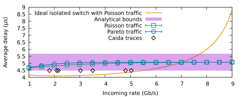
Figure 6: Delay at the second interface when receiving traffic from a single power saving interface.

Finally, we have also tested the performance of tandem networks of variable lengths. The experimental network consists on a regular interface followed by up to 100 power efficient interfaces.

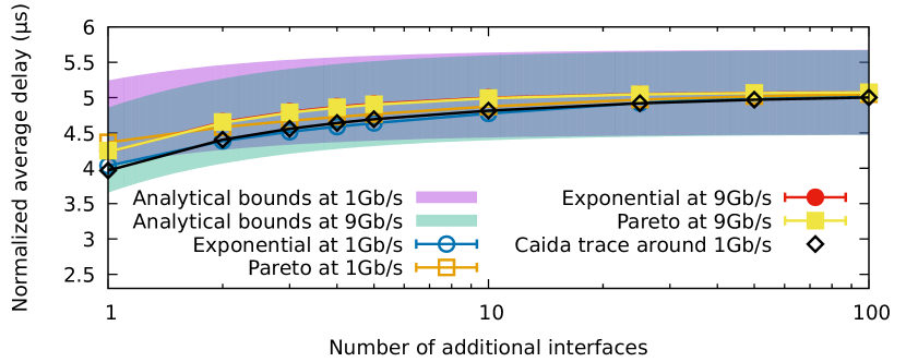
Figure 7: Normalized delay measured on a tandem of $n$ interfaces with different kinds of incoming traffic.

The results in Fig. 7 show that the per interface average delay is between the predicted bounds for different average rates and all kinds of incoming traffic.

V Conclusions

In this paper we have modeled the delay of traffic traversing a series of EEE interfaces. Although the delay of a single interface was already well understood and known to be negligible in most contexts, the study of the effects of the accumulation had been neglected before.

We have proven and empirically tested that, when the traffic to an energy efficient link arrives from several previous interfaces, their arrivals can be modeled with a Poisson process. Therefore, the delay in this scenario can be modeled like in the isolated case, without regarding whether the traffic first traversed energy efficient links, regular links or a mix of them. We have also shown that the delay strictly due to the EEE capabilities of the interface is never larger than the length of the setup time, usually just a few microseconds.

Finally, we have also shown how, when the traffic is dominated by a single contributor, its delay is quite different (and quite smaller) than that of an isolated interface. The delay in these interfaces never grows larger than the setup time plus the transmission time of a single frame. This result helps to calculate budget delays in EEE networks. It is also important to note that this kind of setup does not add any jitter to the traffic as long as the frame sizes are constant.

Future work includes extending the current analysis for the case where the interfaces employ different algorithms to manage the power saving mode, such as the packet coalescing technique, that waits for several frames to arrive while in the LPI mode before returning to the active mode.

References

- [1] “IEEE Std 802.3az-2010 (Amendment to IEEE Std 802.3-2008),” pp. 1–302, 2010. [Online]. Available: http://dx.doi.org/10.1109/IEEESTD.2010.5621025
- [2] “IEEE Std 802.3bj-2014 (Amendment to IEEE Std 802.3-2012 as amended by IEEE Std 802.3bk-2013),” pp. 1–368, 2014.
- [3] P. Reviriego, K. Christensen, J. Rabanillo, and J. A. Maestro, “An Initial Evaluation of Energy Efficient Ethernet,” IEEE Commun. Lett., vol. 15, no. 5, pp. 578–580, may 2011.
- [4] S. Herrería Alonso, M. Rodríguez Pérez, M. Fernández Veiga, and C. López García, “A GI/G/1 Model for 10 Gb/s Energy Efficient Ethernet Links,” IEEE Trans. Commun., vol. 60, no. 11, pp. 3386–3395, nov 2012.
- [5] D. Larrabeiti, P. Reviriego, J. Hernández, J. Maestro, and M. Urueña, “Towards an energy efficient 10 Gb/s optical ethernet: Performance analysis and viability,” Opt. Switch. Netw., vol. 8, no. 3, pp. 131–138, jul 2011.
- [6] A. Cenedese, F. Tramarin, and S. Vitturi, “An Energy Efficient Ethernet Strategy Based on Traffic Prediction and Shaping,” IEEE Trans. Commun., vol. 65, no. 1, pp. 270–282, 2017.
- [7] M. Mostowfi and K. Christensen, “An energy-delay model for a packet coalescer,” in 2012 Proc. IEEE Southeastcon, mar 2012, pp. 1–6.
- [8] K. J. Kim, S. Jin, N. Tian, and B. D. Choi, “Mathematical analysis of burst transmission scheme for IEEE 802.3az energy efficient Ethernet,” Perform. Eval., vol. 70, no. 5, pp. 350–363, may 2013.
- [9] R. Bolla, R. Bruschi, A. Carrega, F. Davoli, and P. Lago, “A closed-form model for the IEEE 802.3az network and power performance,” IEEE J. Sel. Areas Commun., vol. 32, no. 1, pp. 16–27, 2014.
- [10] P. J. Burke, “The Output of a Queuing System,” Oper. Res., vol. 4, no. 6, pp. 699–704, dec 1956.
- [11] NS, “ns Network Simulator,” 2007. [Online]. Available: http://www.isi.edu/nsman/ns/
- [12] “ns Network Simulator v2.35 with IEEE802.3az Support,” 2014. [Online]. Available: https://github.com/migrax/ns2/commits/ieee802.3az
- [13] “The CAIDA UCSD anonymized 2015 Internet traces,” https://www.caida.org/data/passive/passive_2015_dataset.xml.
- [14] D. Murray and T. Koziniec, “The state of enterprise network traffic in 2012,” in 2012 18th Asia-Pacific Conf. Commun., oct 2012, pp. 179–184.