IBVPs for Scalar Conservation Laws
with Time Discontinuous Fluxes

Abstract

The initial boundary value problem for a class of scalar non autonomous conservation laws in one space dimension is proved to be well posed and stable with respect to variations in the flux. Targeting applications to traffic, the regularity assumptions on the flow are extended to a merely ${\mathbf{L}^{\infty}}$ dependence on time. These results ensure, for instance, the well posedness of a class of vehicular traffic models with time dependent speed limits. A traffic management problem is then shown to admit an optimal solution.

2010 Mathematics Subject Classification: 35L65, 35L04

Keywords: Conservation Laws, Boundary Value Problems for Conservation Laws

1 Introduction

In this paper we deal with a non linear Initial Boundary Value Problem (IBVP) for a non autonomous scalar conservation law in one space dimension. Our main result is its well posedness and the stability of solutions with respect to variations in the flux, relaxing the regularity assumptions found in the literature, see for instance [3, 6, 15, 21].

The theory of Conservation Laws traditionally splits in that of scalar multi–dimensional equations and that of one dimensional systems. In the former case, the key reference related to IBVPs is [3], see also [4, 6, 14, 15, 16, 21]. In the latter case, we refer to [1, 7, 8, 10].

Below, we consider the following IBVP both on the (unbounded) half line ${\mathbb{R}}_{+}$

$$\left\{\begin{array}[]{l@{\,}c@{\,}lr@{\,}c@{\,}l}\lx@intercol\partial_{t}u+\partial_{x}\left(v(t)\,g(u)\right)=0\hfil\lx@intercol&(t,x)&\in&[0,T]\times{\mathbb{R}}_{+}\\ u(0,x)&=&u_{o}(x)&x&\in&{\mathbb{R}}_{+}\\ u(t,0)&=&u_{b}(t)&t&\in&[0,T],\end{array}\right.$$ (1.1)

and on the bounded segment $[0,L]$

$$\left\{\begin{array}[]{l@{\,}c@{\,}lr@{\,}c@{\,}l}\lx@intercol\partial_{t}u+\partial_{x}\left(v(t)\,g(u)\right)=0\hfil\lx@intercol&(t,x)&\in&[0,T]\times[0,L]\\ u(0,x)&=&u_{o}(x)&x&\in&[0,L]\\ u(t,0)&=&u_{b,1}(t)&t&\in&[0,T]\\ u(t,L)&=&u_{b,2}(t)&t&\in&[0,T].\end{array}\right.$$ (1.2)

Remark that here the flux is the product between a time dependent function $v(t)$ and a function of the unknown $g(u)$. The time dependent part of the flux is here assumed to be merely ${\mathbf{L}^{\infty}}$ and the domain needs not be bounded, significantly extending what required in [3, 15, 21], where the flow is smooth and the domain is bounded. In [6], the domain can be unbounded but the flow needs be smooth too, although of the more general form $f(t,u)$. Nevertheless, the results in [6, § 2.1 and § 3.1] concerning the autonomous (time independent) problems, that is with flux of the form $f(u)$, constitute the starting point for the present work. Aiming to deal with a merely ${\mathbf{L}^{\infty}}$ function $v$, as an intermediate step we first focus on the case of Lipschitz continuous $v$. Under this assumption, an ad hoc diffeomorphism, transforming (1.1), respectively (1.2), into an autonomous problem of the type considered in [6], allows to extend the well posedness and stability results to the present setting. The stability with respect to the flux, and in particular to $v$, allows then to further relax the regularity assumptions on $v$, up to ${\mathbf{L}^{\infty}}$, without any requirement on the boundedness of the total variation in time.

We adopt the same definition of solution to (1.1), respectively (1.2), as in [6]. As far as bounded domains are concerned, this definition was introduced in [15, 16, 21], see also [14]. As in [6], we also consider the unbounded case of the half line. This definition of solution has the remarkable feature of being stable under convergence in ${\mathbf{L}^{1}}$, see [14, Chapter 2, Remark 7.33] and also [19, Remark 3.6]. This constitutes a crucial element in the proof of the well posedness of problem (1.1) when $v$ is a function in ${\mathbf{L}^{\infty}}$, see Theorem 2.6. We refer to [19] for a deeper discussion of the various definitions of solutions to IBVPs for balance laws.

The well posedness and stability results obtained below suits various issues arising in the macroscopic modelling of vehicular traffic flows. Indeed, we consider in detail the problem of choosing a variable speed limit that minimizes the time spent in queues at a traffic light. We refer to [20] and to the references therein for a more engineering oriented approach, to [5] for further related control and inverse problems.

The paper is organised as follows. Section 2 deals with problem (1.1) on the half line: after providing the definition of solution, § 2.1 presents the results for Lipschitz continuous $v$, while § 2.2 is devoted to the case $v\in{\mathbf{L}^{\infty}}$. Section 3 is structured in a similar way for the IBVP (1.2) on a bounded segment. These results allow to prove the existence of an optimal control for a traffic management problem, see Section 4. All proofs related to the case of the half line are collected in Section 5, where the necessary preliminary results are also recalled.

2 The Case of a Half Line

All statements and proofs are referred to the time interval $[0,T]$, for a fixed positive $T$. Throughout, $v_{\min}$ is a strictly positive constant.

Below, if $u_{\ell}\in{\mathbf{L}^{\infty}}(I_{\ell};{\mathbb{R}})$ for real intervals $I_{\ell}$, $\ell=1,\ldots,m$, we denote

$$\mathcal{U}(u_{1},\ldots,u_{m})=\bigl{[}\min_{\ell=1,\ldots,m}\operatorname*{ess\,inf}_{I_{\ell}}u_{\ell}\,,\;\max_{\ell=1,\ldots,m}\operatorname*{ess\,sup}_{I_{\ell}}u_{\ell}\bigr{]}\,.$$ (2.1)

In other words, $\mathcal{U}(u_{1},\ldots,u_{m})$ is the closed convex hull of $\bigcup_{\ell=1}^{m}u_{\ell}(I_{\ell})$. Whenever $I_{u}$ is a real interval, for $u\in\mathbf{BV}(I_{u};{\mathbb{R}})$, $\mathinner{\rm TV}(u)$ stands for the total variation of $u$ on $I_{u}$, see [9, § 5.10.1], and, for any interval $I\subseteq I_{u}$, we also set $\mathinner{\rm TV}(u;I)=\mathinner{\rm TV}(u_{|I})$. For the vector $\boldsymbol{u}=\left(u_{1},\ldots,u_{m}\right)$, we define $\mathinner{\rm TV}(\boldsymbol{u})=\sum_{\ell=1}^{m}\mathinner{\rm TV}(u_{\ell})$.

The following notation is of use

$$\mathop{\rm sgn}{}^{+}(s)=\ \begin{cases}1&\mbox{ if }s>0,\\ 0&\mbox{ if }s\leq 0,\end{cases} \mathop{\rm sgn}{}^{-}(s)=\ \begin{cases}0&\mbox{ if }s\geq 0,\\ -1&\mbox{ if }s<0,\end{cases} \begin{aligned} s^{+}=\ &\max\{s,0\},\\ s^{-}=\ &\max\{-s,0\}.\end{aligned}$$

Occasionally, we also denote $t_{1}\vee t_{2}=\max\{t_{1},t_{2}\}$.

Definition 2.1.

A solution to the IBVP

$$\left\{\begin{array}[]{l@{\,}c@{\,}lr@{\,}c@{\,}l}\lx@intercol\partial_{t}u+\partial_{x}f(t,u)=0\hfil\lx@intercol&(t,x)&\in&[0,T]\times{\mathbb{R}}_{+}\\ u(0,x)&=&u_{o}(x)&x&\in&{\mathbb{R}}_{+}\\ u(t,0)&=&u_{b}(t)&t&\in&[0,T],\end{array}\right.$$ (2.2)

is a map $u\in{\mathbf{L}^{\infty}}([0,T]\times{\mathbb{R}}_{+};{\mathbb{R}})$ such that for any $k\in{\mathbb{R}}$ and for any test function $\varphi\in\mathbf{C}_{c}^{1}({\mathbb{R}}\times{\mathbb{R}};{\mathbb{R}}_{+})$

$$\int_{0}^{T}\!\!\!\int_{{\mathbb{R}}_{+}}\left\{\left(u(t,x)-k\right)^{\pm}\partial_{t}\varphi(t,x)+\mathop{\rm sgn}{}^{\pm}\!\left(u(t,x)-k\right)\!\left(f\left(t,u(t,x)\right)-f(t,k)\right)\partial_{x}\varphi(t,x)\right\}\mathinner{\mathrm{d}{x}}\mathinner{\mathrm{d}{t}}$$

$$+\int_{{\mathbb{R}}_{+}}\left(u_{o}(x)-k\right)^{\pm}\varphi(0,x)\,\mathinner{\mathrm{d}{x}}-\int_{{\mathbb{R}}_{+}}\left(u(T,x)-k\right)^{\pm}\varphi(T,x)\,\mathinner{\mathrm{d}{x}}$$

$$+{\left\|\partial_{u}f\right\|}_{{\mathbf{L}^{\infty}}([0,T]\times\mathcal{U};{\mathbb{R}})}\int_{0}^{T}\left(u_{b}(t)-k\right)^{\pm}\varphi(t,0)\,\mathinner{\mathrm{d}{t}}\geq 0,$$

where $\mathcal{U}=\mathcal{U}(u_{o},{u_{b}}_{|[0,T]})$ as in (2.1).

The above choice is inspired by [6, Definition 2.1], see also [15, 21] in a slightly different setting. Refer in particular to [19] for a comparison among various definitions of solutions to IBVPs for general scalar balance laws, also in several space dimensions.

2.1 Lipschitz Continuous $\boldsymbol{v}$

This paragraph is devoted to the well posedness of problem (1.1), under the assumptions that the time dependent part of the flux $v$ is in $\mathbf{C}^{0,1}([0,T];[v_{\min},+\infty[)$. All proofs of the results presented below are deferred to § 5.2.

First, we extend [6, Proposition 2.2], see also Proposition 5.1, to the present more general case, i.e. under less regularity assumptions on the flux, obtaining the ${\mathbf{L}^{1}}$–Lipschitz continuous dependence of the solutions on initial and boundary data.

Proposition 2.2.

Let $v\in\mathbf{C}^{0,1}([0,T];[v_{\min},+\infty[)$. Fix $g\in\mathbf{C}^{1}({\mathbb{R}};{\mathbb{R}})$. Let $u_{o},\tilde{u}_{o}\in({\mathbf{L}^{1}}\cap\mathbf{BV})({\mathbb{R}}_{+};{\mathbb{R}})$, $u_{b},\tilde{u}_{b}\in({\mathbf{L}^{1}}\cap\mathbf{BV})([0,T];{\mathbb{R}})$. Assume that the IBVPs

$$\left\{\begin{array}[]{r@{\;}c@{\;}l}\lx@intercol\partial_{t}u+\partial_{x}\left(v(t)\,g(u)\right)=0\hfil\lx@intercol\\ u(0,x)&=&u_{o}(x)\\ u(t,0)&=&u_{b}(t)\end{array}\right.\quad\mbox{ and }\quad\left\{\begin{array}[]{r@{\;}c@{\;}l}\lx@intercol\partial_{t}\tilde{u}+\partial_{x}\left(v(t)\,g(\tilde{u})\right)=0\hfil\lx@intercol\\ \tilde{u}(0,x)&=&\tilde{u}_{o}(x)\\ \tilde{u}(t,0)&=&\tilde{u}_{b}(t)\end{array}\right.$$

admit solutions $u,\tilde{u}\in{\mathbf{L}^{\infty}}([0,T]\times{\mathbb{R}}_{+};{\mathbb{R}})$ in the sense of Definition 2.1, such that $u$ and $\tilde{u}$ both admit a trace for $x\to 0+$ for a.e. $t\in[0,T]$. Then, for all $t\in[0,T]$,

$${\left\|u(t)-\tilde{u}(t)\right\|}_{{\mathbf{L}^{1}}({\mathbb{R}}_{+};{\mathbb{R}})}\leq{\left\|u_{o}-\tilde{u}_{o}\right\|}_{{\mathbf{L}^{1}}({\mathbb{R}}_{+};{\mathbb{R}})}+{\left\|v\right\|}_{{\mathbf{L}^{\infty}}([0,t];{\mathbb{R}})}\,{\left\|g^{\prime}\right\|}_{{\mathbf{L}^{\infty}}(\mathcal{U};{\mathbb{R}})}\,{\left\|u_{b}-\tilde{u}_{b}\right\|}_{{\mathbf{L}^{1}}([0,t];{\mathbb{R}})},$$

where $\mathcal{U}=\mathcal{U}({u_{b}}_{|[0,t]},{\tilde{u}}_{b|[0,t]})$ as in (2.1).

Now, we deal with existence and a priori estimates on solutions to (1.1) in the case of a merely Lipschitz continuous $v$.

Proposition 2.3.

Let $v\in\mathbf{C}^{0,1}([0,T];[v_{\min},+\infty[)$, $g\in{\mathbf{W}_{\mathbf{loc}}^{1,\infty}}({\mathbb{R}};{\mathbb{R}})$, $u_{o}\in({\mathbf{L}^{1}}\cap\mathbf{BV})({\mathbb{R}}_{+};{\mathbb{R}})$ and $u_{b}\in({\mathbf{L}^{1}}\cap\mathbf{BV})([0,T];{\mathbb{R}})$. Then problem (1.1) admits a solution $u$ in the sense of Definition 2.1 with the properties:

1. Range of $u$: with the notation in (2.1), $u(t,x)\in\mathcal{U}(u_{o},{u_{b}}_{|[0,t]})$ for a.e. $(t,x)\in[0,T]\times{\mathbb{R}}_{+}$. Hence, for all $t\in[0,T]$, ${\left\|u(t)\right\|}_{{\mathbf{L}^{\infty}}({\mathbb{R}}_{+};{\mathbb{R}})}\leq\max\left\{{\left\|u_{o}\right\|}_{{\mathbf{L}^{\infty}}({\mathbb{R}}_{+};{\mathbb{R}})},\,{\left\|u_{b}\right\|}_{{\mathbf{L}^{\infty}}([0,t];{\mathbb{R}})}\right\}$.

2. $u$ is ${\mathbf{L}^{1}}$–Lipschitz continuous in time: for all $t_{1},t_{2}\in[0,T]$,

   $${\left\|u(t_{1})-u(t_{2})\right\|}_{{\mathbf{L}^{1}}({\mathbb{R}}_{+};{\mathbb{R}})}\leq\mathinner{\rm TV}(t_{1}\vee t_{2},u_{o},u_{b})\;{\left\|v\right\|}_{{\mathbf{L}^{\infty}}([0,t_{1}\vee t_{2}];{\mathbb{R}})}\,{\left\|g^{\prime}\right\|}_{{\mathbf{L}^{\infty}}(\mathcal{U};{\mathbb{R}})}\,{\left|t_{2}-t_{1}\right|},$$

   where

   $$\mathinner{\rm TV}(t,u_{o},u_{b})=\mathinner{\rm TV}(u_{o})+\mathinner{\rm TV}(u_{b};[0,t])+{\left|u_{b}(0+)-u_{o}(0+)\right|},$$ (2.3)

   and $\mathcal{U}=\mathcal{U}(u_{o},{u_{b}}_{|[0,t_{1}\vee t_{2}]})$, with the notation (2.1).

3. Total variation estimate: for all $t\in[0,T]$, $\mathinner{\rm TV}\left(u(t)\right)\leq\mathinner{\rm TV}(t,u_{o},u_{b})$, with the notation (2.3).

To conclude this paragraph, we ensure the stability with respect to the flux of the solution to (1.1), under the hypothesis $v\in\mathbf{C}^{0,1}([0,T];[v_{\min},+\infty[)$.

Theorem 2.4.

Let $v,\tilde{v}\in\mathbf{C}^{0,1}([0,T];[v_{\min},+\infty[)$. Fix $g,\tilde{g}\in\mathbf{C}^{1}({\mathbb{R}};{\mathbb{R}})$. Let $u_{o}\in({\mathbf{L}^{1}}\cap\mathbf{BV})({\mathbb{R}}_{+};{\mathbb{R}})$, $u_{b}\in({\mathbf{L}^{1}}\cap\mathbf{BV})([0,T];{\mathbb{R}})$. Call $u$ and $\tilde{u}$ the solutions to the IBVPs

$$\left\{\begin{array}[]{r@{\;}c@{\;}l}\lx@intercol\partial_{t}u+\partial_{x}\left(v(t)\,g(u)\right)=0\hfil\lx@intercol\\ u(0,x)&=&u_{o}(x)\\ u(t,0)&=&u_{b}(t)\end{array}\right.\quad\mbox{ and }\qquad\left\{\begin{array}[]{r@{\;}c@{\;}l}\lx@intercol\partial_{t}\tilde{u}+\partial_{x}\left(\tilde{v}(t)\,\tilde{g}(\tilde{u})\right)=0\hfil\lx@intercol\\ \tilde{u}(0,x)&=&u_{o}(x)\\ \tilde{u}(t,0)&=&u_{b}(t).\end{array}\right.$$ (2.4)

where $(t,x)\in[0,T]\times{\mathbb{R}}_{+}$. Then the following estimate holds: for all $t\in[0,T]$

$${\left\|u(t)-\tilde{u}(t)\right\|}_{{\mathbf{L}^{1}}({\mathbb{R}}_{+};{\mathbb{R}})}\leq\mathinner{\rm TV}(t,u_{o},u_{b})\left(A\,t\,{\left\|g^{\prime}-\tilde{g}^{\prime}\right\|}_{{\mathbf{L}^{\infty}}(\mathcal{U};{\mathbb{R}})}+B\,{\left\|v-\tilde{v}\right\|}_{{\mathbf{L}^{1}}([0,t];{\mathbb{R}})}\right),$$ (2.5)

where $\mathinner{\rm TV}(t,u_{o},u_{b})$ is defined in (2.3), $\mathcal{U}=\mathcal{U}(u_{o},{u_{b}}_{|[0,t]})$ is as in (2.1) and

$$\begin{array}[]{r@{\;}l@{\qquad\qquad}r@{\;}l}A=&\max\left\{1,G\right\}\,V,&G=&\min\left\{{\left\|g^{\prime}\right\|}_{{\mathbf{L}^{\infty}}(\mathcal{U};{\mathbb{R}})},{\left\|\tilde{g}^{\prime}\right\|}_{{\mathbf{L}^{\infty}}(\mathcal{U};{\mathbb{R}})}\right\},\\ B=&\left(1+\dfrac{V}{v_{\min}}\right)\,G,&V=&\min\left\{{\left\|v\right\|}_{{\mathbf{L}^{\infty}}([0,t];{\mathbb{R}})},{\left\|\tilde{v}\right\|}_{{\mathbf{L}^{\infty}}([0,t];{\mathbb{R}})}\right\}.\end{array}$$ (2.6)

Remark 2.5.

In the case of a more regular flux function, say $v\in\mathbf{C}^{1}([0,T];[v_{\min},+\infty[)$, also the stability estimate presented in [6, Theorem 2.6] can be applied, obtaining

$${\left\|u(t)-\tilde{u}(t)\right\|}_{{\mathbf{L}^{1}}({\mathbb{R}}_{+};{\mathbb{R}})}\leq\mathinner{\rm TV}(t,u_{o},u_{b})\left(A\,{\left\|g^{\prime}-\tilde{g}^{\prime}\right\|}_{{\mathbf{L}^{\infty}}(\mathcal{U};{\mathbb{R}})}+B\,{\left\|v-\tilde{v}\right\|}_{{\mathbf{L}^{\infty}}([0,t];{\mathbb{R}})}\right)t,$$

with the same notation introduced in (2.6). Clearly, the bound (2.5) is more precise. This improvement plays a key role in the relaxation of the hypothesis on $v$ achieved in Theorem 2.6.

2.2 Discontinuous $\boldsymbol{v}$

Our aim is now to further relax the regularity hypothesis on $v$, allowing also for discontinuous functions. In particular, we set $v\in{\mathbf{L}^{\infty}}([0,T];[v_{\min},+\infty[)$.

Theorem 2.6.

Let $v\in{\mathbf{L}^{\infty}}([0,T];[v_{\min},+\infty[)$, $g\in\mathbf{C}^{1}({\mathbb{R}};{\mathbb{R}})$. Fix $u_{o}\in({\mathbf{L}^{1}}\cap\mathbf{BV})({\mathbb{R}}_{+};{\mathbb{R}})$, $u_{b}\in({\mathbf{L}^{1}}\cap\mathbf{BV})([0,T];{\mathbb{R}})$. Then problem (1.1) admits a solution $u$ in the sense of Definition 2.1 with the properties:

1. Range of $u$: with the notation in (2.1), $u(t,x)\in\mathcal{U}(u_{o},{u_{b}}_{|[0,t]})$ for a.e. $(t,x)\in[0,T]\times{\mathbb{R}}_{+}$. Hence, for all $t\in[0,T]$, ${\left\|u(t)\right\|}_{{\mathbf{L}^{\infty}}({\mathbb{R}}_{+};{\mathbb{R}})}\leq\max\left\{{\left\|u_{o}\right\|}_{{\mathbf{L}^{\infty}}({\mathbb{R}}_{+};{\mathbb{R}})},\,{\left\|u_{b}\right\|}_{{\mathbf{L}^{\infty}}([0,t];{\mathbb{R}})}\right\}$.

2. $u$ is ${\mathbf{L}^{1}}$–Lipschitz continuous in time: for all $t_{1},t_{2}\in[0,T]$,

   $${\left\|u(t_{1})-u(t_{2})\right\|}_{{\mathbf{L}^{1}}({\mathbb{R}}_{+};{\mathbb{R}})}\leq\mathinner{\rm TV}(t_{1}\vee t_{2},u_{o},u_{b})\;{\left\|v\right\|}_{{\mathbf{L}^{\infty}}([0,t_{1}\vee t_{2}];{\mathbb{R}})}\,{\left\|g^{\prime}\right\|}_{{\mathbf{L}^{\infty}}(\mathcal{U};{\mathbb{R}})}\,{\left|t_{2}-t_{1}\right|},$$

   where $\mathinner{\rm TV}(t,u_{o},u_{b})$ is as in (2.3) and $\mathcal{U}=\mathcal{U}(u_{o},{u_{b}}_{|[0,t_{1}\vee t_{2}]})$, with the notation (2.1).

3. Total variation estimate: for $t{\in}[0,T]$, with the notation (2.3), $\mathinner{\rm TV}\left(u(t)\right)\!\leq\!\mathinner{\rm TV}(t,u_{o},u_{b})$.

4. ${\mathbf{L}^{1}}$–Lipschitz continuity on initial and boundary data: if $\tilde{u}_{o}\in({\mathbf{L}^{1}}\cap\mathbf{BV})({\mathbb{R}}_{+};{\mathbb{R}})$, $\tilde{u}_{b}\in({\mathbf{L}^{1}}\cap\mathbf{BV})([0,T];{\mathbb{R}})$ and $\tilde{u}$ is the corresponding solution to (1.1), for all $t\in[0,T]$,

   $${\left\|u(t)-\tilde{u}(t)\right\|}_{{\mathbf{L}^{1}}({\mathbb{R}}_{+};{\mathbb{R}})}\leq{\left\|u_{o}-\tilde{u}_{o}\right\|}_{{\mathbf{L}^{1}}({\mathbb{R}}_{+};{\mathbb{R}})}+{\left\|v\right\|}_{{\mathbf{L}^{\infty}}([0,t];{\mathbb{R}})}{\left\|g^{\prime}\right\|}_{{\mathbf{L}^{\infty}}(\mathcal{U};{\mathbb{R}})}{\left\|u_{b}-\tilde{u}_{b}\right\|}_{{\mathbf{L}^{1}}([0,t];{\mathbb{R}})},$$

   where $\mathcal{U}=\mathcal{U}({u_{b}}_{|[0,t]},{\tilde{u}}_{b|[0,t]})$ as in (2.1).

5. ${\mathbf{L}^{1}}$–stability with respect to $v$ and $g$: if $\tilde{v}\in{\mathbf{L}^{\infty}}([0,T];[v_{\min},+\infty[)$, $\tilde{g}\in\mathbf{C}^{1}({\mathbb{R}};{\mathbb{R}})$ and $\tilde{u}$ is the corresponding solution to (1.1), for all $t\in[0,T]$,

   $${\left\|u(t)-\tilde{u}(t)\right\|}_{{\mathbf{L}^{1}}({\mathbb{R}}_{+};{\mathbb{R}})}\leq\mathinner{\rm TV}(t,u_{o},u_{b})\left(A\,t\,{\left\|g^{\prime}-\tilde{g}^{\prime}\right\|}_{{\mathbf{L}^{\infty}}(\mathcal{U};{\mathbb{R}})}+B\,{\left\|v-\tilde{v}\right\|}_{{\mathbf{L}^{1}}([0,t];{\mathbb{R}})}\right),$$

   where $\mathinner{\rm TV}(t,u_{o},u_{b})$ is defined in (2.3), $\mathcal{U}=\mathcal{U}(u_{o};{u_{b}}_{|[0,t]})$ is as in (2.1) and we use the notation (2.6).

The proof is deferred to § 5.3.

3 The Case of a Segment

In this Section we focus on the IBVP (1.2) where $x$ varies in a segment. We follow the same structure of Section 2 and provide all statements in details, though omitting the proofs, since they are entirely analogous to those presented in § 5.2 and § 5.3 for the case of the half line, now relying on [6, § 3.1].

Consider first the more general IBVP on a segment

$$\left\{\begin{array}[]{l@{\,}c@{\,}lr@{\,}c@{\,}l}\lx@intercol\partial_{t}u+\partial_{x}f(t,u)=0\hfil\lx@intercol&(t,x)&\in&[0,T]\times[0,L]\\ u(0,x)&=&u_{o}(x)&x&\in&[0,L]\\ u(t,0)&=&u_{b,1}(t)&t&\in&[0,T]\\ u(t,L)&=&u_{b,2}(t)&t&\in&[0,T].\end{array}\right.$$ (3.1)

The definition of solution to (3.1) is analogous to Definition 2.1. Here we have one more term, due to the boundary $x=L$.

Definition 3.1.

A solution to the IBVP (3.1) is a map $u\in{\mathbf{L}^{\infty}}([0,T]\times[0,L];{\mathbb{R}})$ such that for any $k\in{\mathbb{R}}$ and for any test function $\varphi\in\mathbf{C}_{c}^{1}({\mathbb{R}}\times{\mathbb{R}};{\mathbb{R}}_{+})$

$$\int_{0}^{T}\!\!\!\int_{0}^{L}\left\{\left(u(t,x)-k\right)^{\pm}\partial_{t}\varphi(t,x)+\mathop{\rm sgn}{}^{\pm}\!\left(u(t,x)-k\right)\!\left(f\left(t,u(t,x)\right)-f(t,k)\right)\partial_{x}\varphi(t,x)\right\}\mathinner{\mathrm{d}{x}}\mathinner{\mathrm{d}{t}}$$

$$+\int_{0}^{L}\left(u_{o}(x)-k\right)^{\pm}\varphi(0,x)\,\mathinner{\mathrm{d}{x}}-\int_{0}^{L}\left(u(T,x)-k\right)^{\pm}\varphi(T,x)\,\mathinner{\mathrm{d}{x}}$$

$$+{\left\|\partial_{u}f\right\|}_{{\mathbf{L}^{\infty}}([0,T]\times\mathcal{U};{\mathbb{R}})}\int_{0}^{T}\left\{\left(u_{b,1}(t)-k\right)^{\pm}\varphi(t,0)+\left(u_{b,2}(t)-k\right)^{\pm}\varphi(t,L)\right\}\mathinner{\mathrm{d}{t}}\geq 0,$$

where $\mathcal{U}=\mathcal{U}(u_{o},{u_{b,1}}_{|[0,T]},{u_{b,2}}_{|[0,T]})$ as in (2.1).

Throughout, we denote $\boldsymbol{u_{b}}=\left(u_{b,1},u_{b,2}\right)$, so that $\mathcal{U}=\mathcal{U}(u_{o},{\boldsymbol{u_{b}}}_{|[0,T]})$.

3.1 Lipschitz continuous $\boldsymbol{v}$

We focus on problem (1.2) under the assumption $v\in\mathbf{C}^{0,1}([0,T];[v_{\min},+\infty[)$.

The following Proposition extends [6, Proposition 3.2] to the present setting of less regularity assumptions on the flux. It is the analogous to Proposition 2.2, but the half line is here replaced by a segment.

Proposition 3.2.

Let $v\in\mathbf{C}^{0,1}([0,T];[v_{\min},+\infty[)$. Fix $g\in\mathbf{C}^{1}({\mathbb{R}};{\mathbb{R}})$. Let $u_{o},\tilde{u}_{o}\in({\mathbf{L}^{1}}\cap\mathbf{BV})([0,L];{\mathbb{R}})$, $\boldsymbol{u_{b}},\boldsymbol{\tilde{u}_{b}}\in({\mathbf{L}^{1}}\cap\mathbf{BV})([0,T];{\mathbb{R}}^{2})$. Assume that the IBVPs

$$\left\{\begin{array}[]{l}\partial_{t}u+\partial_{x}\left(v(t)\,g(u)\right)=0\\ u(0,x)=u_{o}(x)\\ \left(u(t,0),u(t,L)\right)=\boldsymbol{u_{b}}(t)\end{array}\right.\quad\mbox{ and }\quad\left\{\begin{array}[]{l}\partial_{t}\tilde{u}+\partial_{x}\left(v(t)\,g(\tilde{u})\right)=0\\ \tilde{u}(0,x)=\tilde{u}_{o}(x)\\ \left(\tilde{u}(t,0),\tilde{u}(t,L)\right)=\boldsymbol{\tilde{u}_{b}}(t)\end{array}\right.$$

admit solutions $u,\tilde{u}\in{\mathbf{L}^{\infty}}([0,T]\times[0,L];{\mathbb{R}})$ in the sense of Definition 3.1, such that $u$ and $\tilde{u}$ both admit a trace for $x\to 0+$ and at $x\to L-$ for a.e. $t\in[0,T]$. Then, for all $t\in[0,T]$,

$${\left\|u(t)\!-\!\tilde{u}(t)\right\|}_{{\mathbf{L}^{1}}([0,L];{\mathbb{R}})}\leq{\left\|u_{o}\!-\!\tilde{u}_{o}\right\|}_{{\mathbf{L}^{1}}([0,L];{\mathbb{R}})}+{\left\|v\right\|}_{{\mathbf{L}^{\infty}}([0,t];{\mathbb{R}})}{\left\|g^{\prime}\right\|}_{{\mathbf{L}^{\infty}}(\mathcal{U};{\mathbb{R}})}\!\sum_{i=1}^{2}{\left\|u_{b.i}-\tilde{u}_{b,i}\right\|}_{{\mathbf{L}^{1}}([0,t];{\mathbb{R}})},$$

where $\mathcal{U}=\mathcal{U}({\boldsymbol{u_{b}}}_{|[0,t]},\boldsymbol{\tilde{u}_{b}}_{|[0,t]})$ is as in (2.1).

The analogous to Proposition 2.3 reads as follows.

Proposition 3.3.

Let $v\in\mathbf{C}^{0,1}([0,T];[v_{\min},+\infty[)$ and $g\in{\mathbf{W}_{\mathbf{loc}}^{1,\infty}}({\mathbb{R}};{\mathbb{R}})$. Fix $u_{o}\in({\mathbf{L}^{1}}\cap\mathbf{BV})([0,L];{\mathbb{R}})$ and $\boldsymbol{u_{b}}\in({\mathbf{L}^{1}}\cap\mathbf{BV})([0,T];{\mathbb{R}}^{2})$. Then problem (1.2) admits a solution $u$ in the sense of Definition 3.1 with the properties:

1. Range of $u$: with the notation in (2.1), $u(t,x)\in\mathcal{U}(u_{o},{\boldsymbol{u_{b}}}_{|[0,t]})$ for a.e. $(t,x)\in[0,T]\times[0,L]$. Hence, for all $t\in[0,T]$,

   $${\left\|u(t)\right\|}_{{\mathbf{L}^{\infty}}([0,L];{\mathbb{R}})}\leq\max\left\{{\left\|u_{o}\right\|}_{{\mathbf{L}^{\infty}}([0,L];{\mathbb{R}})},\,{\left\|u_{b,1}\right\|}_{{\mathbf{L}^{\infty}}([0,t];{\mathbb{R}})},\,{\left\|u_{b,2}\right\|}_{{\mathbf{L}^{\infty}}([0,t];{\mathbb{R}})}\right\}.$$

2. $u$ is ${\mathbf{L}^{1}}$–Lipschitz continuous in time: for all $t_{1},t_{2}\in[0,T]$,

   $${\left\|u(t_{1})-u(t_{2})\right\|}_{{\mathbf{L}^{1}}([0,L];{\mathbb{R}})}\leq\mathinner{\rm TV}(t_{1}\vee t_{2},u_{o},\boldsymbol{u_{b}})\;{\left\|v\right\|}_{{\mathbf{L}^{\infty}}([0,t_{1}\vee t_{2}];{\mathbb{R}})}\,{\left\|g^{\prime}\right\|}_{{\mathbf{L}^{\infty}}(\mathcal{U};{\mathbb{R}})}\,{\left|t_{2}-t_{1}\right|},$$

   where

   $$\mathinner{\rm TV}(t,u_{o},\boldsymbol{u_{b}}){=}\mathinner{\rm TV}(u_{o})+\mathinner{\rm TV}(\boldsymbol{u_{b}};[0,t])+{\left|u_{b,1}(0+)-u_{o}(0+)\right|}+{\left|u_{b,2}(0+)-u_{o}(L-)\right|},$$ (3.2)

   and $\mathcal{U}=\mathcal{U}(u_{o},{\boldsymbol{u_{b}}}_{|[0,t_{1}\vee t_{2}]})$, with the notation (2.1).

3. Total variation estimate: for all $t\in[0,T]$, $\mathinner{\rm TV}\left(u(t)\right)\leq\mathinner{\rm TV}(t,u_{o},\boldsymbol{u_{b}})$, with the notation (3.2).

We conclude this paragraph with the following Theorem, stating the stability with respect to the flux of the solution to (1.2), under the hypothesis $v\in\mathbf{C}^{0,1}([0,T];[v_{\min},+\infty[)$.

Theorem 3.4.

Let $v,\tilde{v}\in\mathbf{C}^{0,1}([0,T];[v_{\min},+\infty[)$. Fix $g,\tilde{g}\in\mathbf{C}^{1}({\mathbb{R}};{\mathbb{R}})$. Let $u_{o}\in({\mathbf{L}^{1}}\cap\mathbf{BV})([0,L];{\mathbb{R}})$, $\boldsymbol{u_{b}}\in({\mathbf{L}^{1}}\cap\mathbf{BV})([0,T];{\mathbb{R}}^{2})$. Call $u$ and $\tilde{u}$ the solutions to the IBVP (1.2), with flux $v\,g$ and $\tilde{v}\,\tilde{g}$ respectively. Then the following estimate holds: for all $t\in[0,T]$

$${\left\|u(t)-\tilde{u}(t)\right\|}_{{\mathbf{L}^{1}}([0,L];{\mathbb{R}})}\leq\mathinner{\rm TV}(t,u_{o},\boldsymbol{u_{b}})\left(A\,t\,{\left\|g^{\prime}-\tilde{g}^{\prime}\right\|}_{{\mathbf{L}^{\infty}}(\mathcal{U};{\mathbb{R}})}+B\,{\left\|v-\tilde{v}\right\|}_{{\mathbf{L}^{1}}([0,t];{\mathbb{R}})}\right),$$

where $\mathinner{\rm TV}(t,u_{o},\boldsymbol{u_{b}})$ is defined in (3.2), $\mathcal{U}=\mathcal{U}(u_{o};{\boldsymbol{u_{b}}}_{|[0,t]})$ is as in (2.1), $A$ and $B$ are defined in (2.6).

3.2 Discontinuous $\boldsymbol{v}$

We now relax the regularity hypothesis on $v$, allowing also for discontinuous functions. In particular, we consider problem (1.2) with $v\in{\mathbf{L}^{\infty}}([0,T];[v_{\min},+\infty[)$.

Theorem 3.5.

Let $v\in{\mathbf{L}^{\infty}}([0,T];[v_{\min},+\infty[)$, $g\in\mathbf{C}^{1}({\mathbb{R}};{\mathbb{R}})$, $u_{o}\in({\mathbf{L}^{1}}\cap\mathbf{BV})([0,L];{\mathbb{R}})$ and $\boldsymbol{u_{b}}\in({\mathbf{L}^{1}}\cap\mathbf{BV})([0,T];{\mathbb{R}}^{2})$. Then problem (1.2) admits a solution $u$ in the sense of Definition 3.1 with the properties:

1. Range of $u$: with the notation in (2.1), $u(t,x)\in\mathcal{U}(u_{o},{\boldsymbol{u_{b}}}_{|[0,t]})$ for a.e. $(t,x)\in[0,T]\times[0,L]$. Hence, for all $t\in[0,T]$,

   $${\left\|u(t)\right\|}_{{\mathbf{L}^{\infty}}([0,L];{\mathbb{R}})}\leq\max\left\{{\left\|u_{o}\right\|}_{{\mathbf{L}^{\infty}}([0,L];{\mathbb{R}})},\,{\left\|u_{b,1}\right\|}_{{\mathbf{L}^{\infty}}([0,t];{\mathbb{R}})},\,{\left\|u_{b,2}\right\|}_{{\mathbf{L}^{\infty}}([0,t];{\mathbb{R}})}\right\}.$$

2. $u$ is ${\mathbf{L}^{1}}$–Lipschitz continuous in time: for all $t_{1},t_{2}\in[0,T]$,

   $${\left\|u(t_{1})-u(t_{2})\right\|}_{{\mathbf{L}^{1}}([0,L];{\mathbb{R}})}\leq\mathinner{\rm TV}(t_{1}\vee t_{2},u_{o},\boldsymbol{u_{b}})\;{\left\|v\right\|}_{{\mathbf{L}^{\infty}}([0,t_{1}\vee t_{2}];{\mathbb{R}})}\,{\left\|g^{\prime}\right\|}_{{\mathbf{L}^{\infty}}(\mathcal{U};{\mathbb{R}})}\,{\left|t_{2}-t_{1}\right|},$$

   where $\mathinner{\rm TV}(t,u_{o},\boldsymbol{u_{b}})$ is as in (3.2) and $\mathcal{U}=\mathcal{U}(u_{o},{\boldsymbol{u_{b}}}_{|[0,t_{1}\vee t_{2}]})$, with the notation (2.1).

3. Total variation estimate: for all $t\in[0,T]$, with the notation (2.3), $\mathinner{\rm TV}\left(u(t)\right)\leq\mathinner{\rm TV}(t,u_{o},\boldsymbol{u_{b}})$, where $\mathinner{\rm TV}(t,u_{o},\boldsymbol{u_{b}})$ is as in (3.2).

4. ${\mathbf{L}^{1}}$–Lipschitz continuity on initial and boundary data: if $\tilde{u}_{o}\in({\mathbf{L}^{1}}\cap\mathbf{BV})([0,L];{\mathbb{R}})$, $\boldsymbol{\tilde{u}_{b}}\in({\mathbf{L}^{1}}\cap\mathbf{BV})([0,T];{\mathbb{R}}^{2})$ and $\tilde{u}$ is the corresponding solution to (1.2), for all $t\in[0,T]$,

   $${\left\|u(t)\!-\!\tilde{u}(t)\right\|}_{{\mathbf{L}^{1}}([0,L];{\mathbb{R}})}\leq\ {\left\|u_{o}\!-\!\tilde{u}_{o}\right\|}_{{\mathbf{L}^{1}}([0,L];{\mathbb{R}})}$$

   $$+{\left\|v\right\|}_{{\mathbf{L}^{\infty}}([0,t];{\mathbb{R}})}{\left\|g^{\prime}\right\|}_{{\mathbf{L}^{\infty}}(\mathcal{U};{\mathbb{R}})}\sum_{i=1}^{2}{\left\|u_{b.i}-\tilde{u}_{b,i}\right\|}_{{\mathbf{L}^{1}}([0,t];{\mathbb{R}})},$$

   where $\mathcal{U}=\mathcal{U}({\boldsymbol{u_{b}}}_{|[0,t]},\boldsymbol{\tilde{u}_{b}}_{|[0,t]})$ as in (2.1).

5. ${\mathbf{L}^{1}}$–stability with respect to $v$ and $g$: if $\tilde{v}\in{\mathbf{L}^{\infty}}([0,T];[v_{\min},+\infty[)$, $\tilde{g}\in\mathbf{C}^{1}({\mathbb{R}};{\mathbb{R}})$ and $\tilde{u}$ is the corresponding solution to (1.2), for all $t\in[0,T]$,

   $${\left\|u(t)-\tilde{u}(t)\right\|}_{{\mathbf{L}^{1}}([0,L];{\mathbb{R}})}\leq\mathinner{\rm TV}(t,u_{o},\boldsymbol{u_{b}})\left(A\,t\,{\left\|g^{\prime}-\tilde{g}^{\prime}\right\|}_{{\mathbf{L}^{\infty}}(\mathcal{U};{\mathbb{R}})}+B\,{\left\|v-\tilde{v}\right\|}_{{\mathbf{L}^{1}}([0,t];{\mathbb{R}})}\right),$$

   where $\mathinner{\rm TV}(t,u_{o},\boldsymbol{u_{b}})$ is defined in (3.2), $\mathcal{U}=\mathcal{U}(u_{o};{\boldsymbol{u_{b}}}_{|[0,t]})$ is as in (2.1) and we use the notation (2.6).

4 Application to Vehicular Traffic

We consider below sample numerical integrations of (1.2). In the interior of the interval $[0,L]$, we employ the standard Lax–Friedrichs method [12, § 4.6]. Along the boundary, we implement the Bardos, le Roux and Nédélec [3] boundary condition in the form [4, Proposition 2.3].

Consider a road segment of length $L=250\,\mbox{m}$. Assume that at the initial time the road is empty, that is to say, the initial datum $u_{o}$ is equal to zero. At the entry of the road, a traffic light remains green for $39\,\mbox{sec}$, while it displays red for $27\,\mbox{sec}$ and, right at time $t=0$, the traffic light turns green. Whenever the traffic light is green, the inflow is $2000\,\mbox{cars}/\mbox{hour}$, see [18, § 6.2] for more details on assigning the inflow as boundary datum. At the end of this road, a second traffic light regulates the outflow, being green for $30\,\mbox{sec}$, red for $45\,\mbox{sec}$, and first turning red at time $t=12\,\mbox{sec}$.

We describe the dynamics of traffic through the Lighthill–Whitham [13] and Richards [17] model with time dependent maximal speed, which amounts to (1.2) with

$$g(u)=u\left(1-\frac{u}{R}\right),$$ (4.1)

$R$ being the maximal possible density, which is here considered to be $200\,\mbox{cars}/\mbox{km}$. Concerning the time dependent (possibly discontinuous) maximal speed $v(t)$, we let

$$v(t)=\begin{cases}60\,\mbox{km}/\mbox{hour}&\mbox{ if traffic light at $x=L$ is green,}\\ V&\mbox{ if traffic light at $x=L$ is red,}\end{cases}$$ (4.2)

where $V$ takes the values

$$40\ \dfrac{\mbox{km}}{\mbox{hour}}, 45\ \dfrac{\mbox{km}}{\mbox{hour}}, 50\ \dfrac{\mbox{km}}{\mbox{hour}}, 55\ \dfrac{\mbox{km}}{\mbox{hour}}, 60\ \dfrac{\mbox{km}}{\mbox{hour}}, 65\ \dfrac{\mbox{km}}{\mbox{hour}}, 70\ \dfrac{\mbox{km}}{\mbox{hour}}.$$ (4.3)

These choices describe possible behaviours of drivers, reacting to the traffic light in front of them either accelerating or slowing down. To allow for reasonable comparisons among the different solutions, we keep throughout the same inflow through the traffic light at $x=0$ as well as the same outflow through the traffic light at $x=L$. As a consequence, the global travel time, i.e. the time necessary to empty the road, is the same in all integrations. Note that the chosen inflow of $2000\,\mbox{cars/hour}$ does not allow choices of the maximal speed lower than $40\,\mbox{km/hour}$.

Remark, that the analytic setting presented in § 3.2 applies, in particular, to the (possibly) discontinuous choice (4.2). Therefore, the resulting model (1.2)–(4.1)–(4.2) is well posed.

To measure the queues formed due to the traffic light at $x=L$, introduce the functional

$$J=\int_{0}^{T}\int_{L-\delta}^{L}\Psi\left(u(t,x)\right)\mathinner{\mathrm{d}{x}}\mathinner{\mathrm{d}{t}},\qquad\mbox{ where }\quad\delta=100\,\mbox{m}$$ (4.4)

$$\Psi(r)=\begin{cases}0&\mbox{ if }r<0.75\,R,\\[3.0pt] \dfrac{10\,r}{R}-7.5&\mbox{ if }0.75\,R\leq r\leq 0.85\,R,\\[3.0pt] 1&\mbox{ if }0.85\,R<r\leq R.\end{cases}$$ (4.5)

The function $\Psi$ weights $1$ wherever the traffic density is above $85\%$ of the maximal density $R$, while it weights $0$ wherever the vehicular density is lower than $75\%$ of $R$.

The values of $J$ resulting from the numerical integration of (1.2)–(4.1)–(4.2), in the different cases (4.3), are shown in Figure 1.

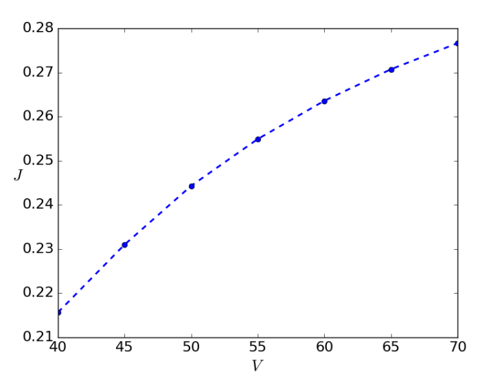
Figure 1: Values of $J$ as defined in (4.4), resulting from the integration of (1.2)–(4.1)–(4.2), for $V$ varying as in (4.3), with zero initial datum, while inflow and outflow are governed by traffic lights as specified in the text.

Note that the results in § 3.2 apply to the present setting and ensure the continuous dependence of $J$ on the parameter $V$. Indeed, the map $V\to u$, where $u$ solves (1.2)–(4.1)–(4.2), is continuous with respect to the ${\mathbf{L}^{1}}$ distance by Theorem 3.5. The continuity of the map $u\to J$ is immediate.

The best choice is clearly the one that corresponds to $V=40\,\mbox{km/hour}$. The qualitative difference in the evolution corresponding to the choices $V=40\,\mbox{km/hour}$ and $V=70\,\mbox{km/hour}$ is displayed in Figure 2.

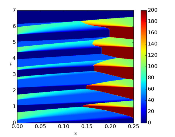
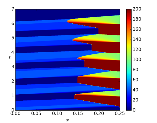
Figure 2: Numerical integration of (1.2)–(4.1)–(4.2), left with $V=40\,\mbox{km/hour}$ and, right, with $V=70\,\mbox{km/hour}$. The initial datum is zero, inflow and outflow are both governed by traffic lights as specified in the text.

These graphs confirm that the speed reductions allows to reduce the queue lengths.

5 Technical Proofs

5.1 Preliminary Results

We recall below the Lipschitz continuous dependence of the solution to (2.2) on initial and boundary data.

Proposition 5.1 ([6, Proposition 2.2]).

Let $f\in\mathbf{C}^{1}([0,T]\times{\mathbb{R}};{\mathbb{R}})$ be such that the map $\{u\mapsto\partial_{t}f(t,u)\}\in{\mathbf{W}_{\mathbf{loc}}^{1,\infty}}({\mathbb{R}};{\mathbb{R}})$ for all $t\in[0,T]$, $u_{o},\tilde{u}_{o}\in({\mathbf{L}^{1}}\cap\mathbf{BV})({\mathbb{R}}_{+};{\mathbb{R}})$ and $u_{b},\tilde{u}_{b}\in({\mathbf{L}^{1}}\cap\mathbf{BV})([0,T];{\mathbb{R}})$. Assume the problems

$$\!\!\!\left\{\begin{array}[]{@{\,}l@{\,}c@{\,}lr@{\,}c@{\,}l}\lx@intercol\partial_{t}u+\partial_{x}f(t,u)=0\hfil\lx@intercol&(t,x)&\in&[0,T]\times{\mathbb{R}}_{+}\\ u(0,x)&=&u_{o}(x)&x&\in&{\mathbb{R}}_{+}\\ u(t,0)&=&u_{b}(t)&t&\in&[0,T]\end{array}\right.\mbox{ and }\left\{\begin{array}[]{@{\,}l@{\,}c@{\,}lr@{\,}c@{\,}l}\lx@intercol\partial_{t}\tilde{u}+\partial_{x}f(t,\tilde{u})=0\hfil\lx@intercol&(t,x)&\in&[0,T]\times{\mathbb{R}}_{+}\\ \tilde{u}(0,x)&=&\tilde{u}_{o}(x)&x&\in&{\mathbb{R}}_{+}\\ \tilde{u}(t,0)&=&\tilde{u}_{b}(t)&t&\in&[0,T]\end{array}\right.\!\!$$

admit solutions $u,\tilde{u}\in{\mathbf{L}^{\infty}}([0,T]\times{\mathbb{R}}_{+};{\mathbb{R}})$ in the sense of Definition 2.1, such that $u$ and $\tilde{u}$ both admit a trace for $x\to 0+$ for a.e. $t\in[0,T]$. Then, for all $t\in[0,T]$,

$${\left\|u(t)-\tilde{u}(t)\right\|}_{{\mathbf{L}^{1}}({\mathbb{R}}_{+};{\mathbb{R}})}\leq{\left\|u_{o}-\tilde{u}_{o}\right\|}_{{\mathbf{L}^{1}}({\mathbb{R}}_{+};{\mathbb{R}})}+{\left\|\partial_{u}f\right\|}_{{\mathbf{L}^{\infty}}([0,t]\times\mathcal{U};{\mathbb{R}})}\;{\left\|u_{b}-\tilde{u}_{b}\right\|}_{{\mathbf{L}^{1}}([0,t];{\mathbb{R}})}$$

where $\mathcal{U}=\mathcal{U}({u_{b}}_{|[0,t]},\,{\tilde{u}}_{b|[0,t]})$ is as in (2.1).

Remark that Proposition 5.1 also ensures the uniqueness of the solution to (2.2) in the sense of Definition 2.1, as soon as a solution exists.

Focus now on the particular case of the autonomous IBVP on the half line:

$$\left\{\begin{array}[]{@{\,}l@{\,}c@{\,}lr@{\,}c@{\,}l}\lx@intercol\partial_{t}u+\partial_{x}g(u)=0\hfil\lx@intercol&(t,x)&\in&[0,T]\times{\mathbb{R}}_{+}\\ u(0,x)&=&u_{o}(x)&x&\in&{\mathbb{R}}_{+}\\ u(t,0)&=&u_{b}(t)&t&\in&[0,T]\,.\end{array}\right.$$ (5.1)

As a definition of solution to (5.1), we consider Definition 2.1 discarding the explicit dependence of the flux on time $t$.

Proposition 5.2 ([6, Proposition 2.3]).

Let $g\in{\mathbf{W}_{\mathbf{loc}}^{1,\infty}}({\mathbb{R}};{\mathbb{R}})$, $u_{o}\in({\mathbf{L}^{1}}\cap\mathbf{BV})({\mathbb{R}}_{+};{\mathbb{R}})$ and $u_{b}\in({\mathbf{L}^{1}}\cap\mathbf{BV})([0,T];{\mathbb{R}})$. Then problem (5.1) admits a solution $u$ in the sense of Definition 2.1, with the properties:

1. If $u_{o}$ and $u_{b}$ are piecewise constant, then for $t$ small, the map $t\to u(t)$ coincides with the gluing of Lax solutions to Riemann problems at the points of jumps of $u_{o}$ and at $x=0$.

2. Range of $u$: with the notation in (2.1), $u(t,x)\in\mathcal{U}(u_{o},{u_{b}}_{|[0,t]})$ for a.e. $(t,x)\in[0,T]\times{\mathbb{R}}_{+}$. Hence, for all $t\in[0,T]$, ${\left\|u(t)\right\|}_{{\mathbf{L}^{\infty}}({\mathbb{R}}_{+};{\mathbb{R}})}\leq\max\left\{{\left\|u_{o}\right\|}_{{\mathbf{L}^{\infty}}({\mathbb{R}}_{+};{\mathbb{R}})},\,{\left\|u_{b}\right\|}_{{\mathbf{L}^{\infty}}([0,t];{\mathbb{R}})}\right\}$.

3. $u$ is ${\mathbf{L}^{1}}$–Lipschitz continuous in time: for all $t_{1},t_{2}\in[0,T]$,

   $${\left\|u(t_{1})-u(t_{2})\right\|}_{{\mathbf{L}^{1}}({\mathbb{R}}_{+};{\mathbb{R}})}\leq\ \mathinner{\rm TV}(t_{1}\vee t_{2},u_{o},u_{b})\;{\left\|g^{\prime}\right\|}_{{\mathbf{L}^{\infty}}(\mathcal{U};{\mathbb{R}})}\;{\left|t_{2}-t_{1}\right|},$$

   with the notation (2.3) and $\mathcal{U}=\mathcal{U}(u_{o},{u_{b}}_{|[0,t_{1}\vee t_{2}]})$, according to (2.1).

4. Total variation estimate: for $t{\in}[0,T]$, with the notation (2.3), $\mathinner{\rm TV}\left(u(t)\right){\leq}\mathinner{\rm TV}(t,u_{o},u_{b})$.

Theorem 5.3 ([6, Theorem 2.4]).

Let $g,\tilde{g}\in\mathbf{C}^{1}({\mathbb{R}};{\mathbb{R}})$, $u_{o}\in({\mathbf{L}^{1}}\cap\mathbf{BV})({\mathbb{R}}_{+};{\mathbb{R}})$ and $u_{b}\in({\mathbf{L}^{1}}\cap\mathbf{BV})([0,T];{\mathbb{R}})$. Call $u$ and $\tilde{u}$ the solutions to the problems

$$\!\!\!\left\{\begin{array}[]{l@{\,}c@{\,}lr@{\,}c@{\,}l}\lx@intercol\partial_{t}u+\partial_{x}g(u)=0\hfil\lx@intercol&(t,x)&\in&[0,T]\times{\mathbb{R}}_{+}\\ u(0,x)&=&u_{o}(x)&x&\in&{\mathbb{R}}_{+}\\ u(t,0)&=&u_{b}(t)&t&\in&[0,T]\end{array}\right.\mbox{ and }\left\{\begin{array}[]{l@{\,}c@{\,}lr@{\,}c@{\,}l}\lx@intercol\partial_{t}\tilde{u}+\partial_{x}\tilde{g}(\tilde{u})=0\hfil\lx@intercol&(t,x)&\in&[0,T]\times{\mathbb{R}}_{+}\\ \tilde{u}(0,x)&=&u_{o}(x)&x&\in&{\mathbb{R}}_{+}\\ \tilde{u}(t,0)&=&u_{b}(t)&t&\in&[0,T]\end{array}\right.\!\!$$

constructed in Proposition 5.2. Then, with $\mathcal{U}=\mathcal{U}(u_{o},{u_{b}}_{|[0,t]})$ as in (2.1), for all $t\in[0,T]$,

$${\left\|u(t)-\tilde{u}(t)\right\|}_{{\mathbf{L}^{1}}({\mathbb{R}}_{+};{\mathbb{R}})} \leq \max\left\{1,G\right\}\,\mathinner{\rm TV}(t,u_{o},u_{b})\,{\left\|g^{\prime}-\tilde{g}^{\prime}\right\|}_{{\mathbf{L}^{\infty}}(\mathcal{U};{\mathbb{R}})}\,t,$$

with $\mathinner{\rm TV}(t,u_{o},u_{b})$ as in (2.3) and $G=\min\left\{{\left\|g^{\prime}\right\|}_{{\mathbf{L}^{\infty}}(\mathcal{U};{\mathbb{R}})},{\left\|\tilde{g}^{\prime}\right\|}_{{\mathbf{L}^{\infty}}(\mathcal{U};{\mathbb{R}})}\right\}$.

5.2 Proofs Related to the Case $v$ Lipschitz Continuous

Let $v\in\mathbf{C}^{0,1}([0,T];[v_{\min},+\infty[)$ and let $\hat{T}=\int_{0}^{T}v(\tau)\mathinner{\mathrm{d}{\tau}}$. Define the bijective map $\Gamma\colon[0,\hat{T}]\to[0,T]$ through its inverse

$$\Gamma^{-1}(t)=\int_{0}^{t}v(s)\mathinner{\mathrm{d}{s}}$$ (5.2)

so that

$$\Gamma^{\prime}(\tau)\;v\left(\Gamma(\tau)\right)=1\,,\qquad(\Gamma^{-1})^{\prime}(t)=v(t)\,,\quad\Gamma(0)=0\quad\mbox{ and }\quad\Gamma(\hat{T})=T\,.$$ (5.3)

We now establish the equivalence between the non autonomous problem (1.1) and an autonomous problem of type (5.1). Throughout, by solution we mean solution in the sense of Definition 2.1.

Lemma 5.4.

Let $v\in\mathbf{C}^{0,1}([0,T];[v_{\min},+\infty[)$ and $g\in\mathbf{C}^{1}({\mathbb{R}};{\mathbb{R}})$. Define $\Gamma$ as in (5.2). Then, if $u$ solves (1.1) the map

$$w(\tau,x)=u\left(\Gamma(\tau),x\right)$$ (5.4)

solves

$$\left\{\begin{array}[]{r@{\;}c@{\;}l@{\qquad}r@{\,}c@{\,}l}\lx@intercol\partial_{\tau}w+\partial_{x}g(w)=0\hfil\lx@intercol&(\tau,x)&\in&[0,\hat{T}]\times{\mathbb{R}}_{+}\\ w(0,x)&=&u_{o}(x)&x&\in&{\mathbb{R}}_{+}\\ w(\tau,0)&=&w_{b}(\tau)&\tau&\in&[0,\hat{T}],\end{array}\right.$$ (5.5)

where $w_{b}(\tau)=u_{b}\left(\Gamma(\tau)\right)$. Conversely, if $w$ solves (5.5), then the map

$$u(t,x)=w(\Gamma^{-1}(t),x)$$ (5.6)

solves (1.1), where $u_{b}(t)=w_{b}\left(\Gamma^{-1}(t)\right)$.

Proof.  For any $\varphi\in\mathbf{C}_{c}^{1}({\mathbb{R}}\times{\mathbb{R}};{\mathbb{R}}_{+})$ and for any $k\in{\mathbb{R}}$, compute the quantity

$$\mathcal{A}=\ \int_{0}^{\hat{T}}\int_{{\mathbb{R}}_{+}}\left(w(\tau,x)-k\right)^{\pm}\partial_{\tau}\varphi(\tau,x)\mathinner{\mathrm{d}{x}}\mathinner{\mathrm{d}{\tau}}$$

$$+\int_{0}^{\hat{T}}\int_{{\mathbb{R}}_{+}}\mathop{\rm sgn}{}^{\pm}\left(w(\tau,x)-k\right)\,\left(g\left(w(\tau,x)\right)-g(k)\right)\,\partial_{x}\varphi(\tau,x)\mathinner{\mathrm{d}{x}}\mathinner{\mathrm{d}{\tau}}$$

$$+\int_{0}^{\hat{T}}\mathop{\rm sgn}{}^{\pm}\left(u_{b}\left(\Gamma(\tau)\right)-k\right)\,\left(g\left(w(\tau,0+)\right)-g(k)\right)\,\varphi(\tau,0+)\mathinner{\mathrm{d}{\tau}}$$

$$+\int_{{\mathbb{R}}_{+}}\left(u_{o}(x)-k\right)^{\pm}\varphi(0,x)\mathinner{\mathrm{d}{x}}-\int_{{\mathbb{R}}_{+}}\left(w(\hat{T},x)-k\right)^{\pm}\varphi(\hat{T},x)\mathinner{\mathrm{d}{x}}$$

$$=\ \int_{0}^{\hat{T}}\int_{{\mathbb{R}}_{+}}\left(u\left(\Gamma(\tau),x\right)-k\right)^{\pm}\partial_{\tau}\varphi(\tau,x)\mathinner{\mathrm{d}{x}}\mathinner{\mathrm{d}{\tau}}$$

$$+\int_{0}^{\hat{T}}\int_{{\mathbb{R}}_{+}}\mathop{\rm sgn}{}^{\pm}\left(u\left(\Gamma(\tau),x\right)-k\right)\left(g\left(u(\Gamma(\tau),x)\right)-g(k)\right)\,\partial_{x}\varphi(\tau,x)\mathinner{\mathrm{d}{x}}\mathinner{\mathrm{d}{\tau}}$$

$$+\int_{0}^{\hat{T}}\mathop{\rm sgn}{}^{\pm}\left(u_{b}\left(\Gamma(\tau)\right)-k\right)\,\left(g\left(u\left(\Gamma(\tau),0+\right)\right)-g(k)\right)\,\varphi(\tau,0+)\mathinner{\mathrm{d}{\tau}}$$

$$+\int_{{\mathbb{R}}_{+}}\left(u_{o}(x)-k\right)^{\pm}\varphi(0,x)\mathinner{\mathrm{d}{x}}-\int_{{\mathbb{R}}_{+}}\left(u\left(\Gamma(\hat{T}),x\right)-k\right)^{\pm}\varphi(\hat{T},x)\mathinner{\mathrm{d}{x}}.$$

Use now the change of variable $\Gamma(\tau)=t$ and define $\psi(t,x)=\varphi\left(\Gamma^{-1}(t),x\right)$. Clearly, $\psi\in\mathbf{C}_{c}^{1}({\mathbb{R}}\times{\mathbb{R}};{\mathbb{R}}_{+})$. Using the properties (5.3) of the function $\Gamma$, continue the computation:

$$\mathcal{A}= \int_{0}^{T}\int_{{\mathbb{R}}_{+}}\left(u\left(t,x\right)-k\right)^{\pm}\,\partial_{t}\psi\left(t,x\right)\mathinner{\mathrm{d}{x}}\mathinner{\mathrm{d}{t}}$$

$$+\int_{0}^{T}\int_{{\mathbb{R}}_{+}}\mathop{\rm sgn}{}^{\pm}\left(u\left(t,x\right)-k\right)\,\left(g\left(u\left(t,x\right)\right)-g(k)\right)v(t)\,\partial_{x}\psi\left(t,x\right)\mathinner{\mathrm{d}{x}}\mathinner{\mathrm{d}{t}}$$

$$+\int_{0}^{T}\mathop{\rm sgn}{}^{\pm}\left(u_{b}\left(t\right)-k\right)\,\left(g\left(u\left(t,0+\right)\right)-g(k)\right)v(t)\,\psi\left(t,0+\right)\mathinner{\mathrm{d}{t}}$$

$$+\int_{{\mathbb{R}}_{+}}\left(u_{o}(x)-k\right)^{\pm}\psi(0,x)\mathinner{\mathrm{d}{x}}-\int_{{\mathbb{R}}_{+}}\left(u\left(T,x\right)-k\right)^{\pm}\psi\left(T,x\right)\mathinner{\mathrm{d}{x}}.$$

Therefore, $u$ is a solution to (1.1) on $[0,T]$ in the sense of Definition 2.1 if and only if $w$ is a solution to (5.5) on $[0,\hat{T}]$ in the sense of Definition 2.1.   $\square$

Proof of Proposition 2.2.  Call $w$ and $\tilde{w}$ the solutions to (5.5) corresponding to $u$ and $\tilde{u}$, respectively, through the relation defined by Lemma 5.4. For all $t\in[0,T]$, use (5.6) and apply Proposition 5.1 to $w$ and $\tilde{w}$:

$${\left\|u(t)-\tilde{u}(t)\right\|}_{{\mathbf{L}^{1}}({\mathbb{R}}_{+};{\mathbb{R}})}=\ {\left\|w(\Gamma^{-1}(t))-\tilde{w}(\Gamma^{-1}(t))\right\|}_{{\mathbf{L}^{1}}({\mathbb{R}}_{+};{\mathbb{R}})}$$

$$\leq\ {\left\|w_{o}-\tilde{w}_{o}\right\|}_{{\mathbf{L}^{1}}({\mathbb{R}}_{+};{\mathbb{R}})}+{\left\|g^{\prime}\right\|}_{{\mathbf{L}^{\infty}}(\mathcal{U};{\mathbb{R}})}{\left\|w_{b}-\tilde{w}_{b}\right\|}_{{\mathbf{L}^{1}}([0,\Gamma^{-1}(t)];{\mathbb{R}})}$$

$$\leq\ {\left\|u_{o}-\tilde{u}_{o}\right\|}_{{\mathbf{L}^{1}}({\mathbb{R}}_{+};{\mathbb{R}})}+{\left\|g^{\prime}\right\|}_{{\mathbf{L}^{\infty}}(\mathcal{U};{\mathbb{R}})}{\left\|v\right\|}_{{\mathbf{L}^{\infty}}([0,t];{\mathbb{R}})}{\left\|u_{b}-\tilde{u}_{b}\right\|}_{{\mathbf{L}^{1}}([0,t];{\mathbb{R}})},$$

where $\mathcal{U}=\mathcal{U}\left({w_{b}}_{|[0,\Gamma^{-1}(t)]},{\tilde{w}}_{b|[0,\Gamma^{-1}(t)]}\right)=\mathcal{U}\left({u_{b}}_{|[0,t]},{\tilde{u}}_{b|[0,t]}\right)$, and this concludes the proof.   $\square$

Proof of Proposition 2.3.  The existence of solutions follows from Lemma 5.4, that allows to apply Proposition 5.2.

In each of the steps below we exploit the correspondence $\Gamma$ and the result of Lemma 5.4.

1. ${\mathbf{L}^{\infty}}$–bound.

Thanks to (5.6) and to Point 2. in Proposition 5.2, for $t\in[0,T]$ we have

$${\left\|u(t)\right\|}_{{\mathbf{L}^{\infty}}({\mathbb{R}}_{+};{\mathbb{R}})}={\left\|w(\Gamma^{-1}(t))\right\|}_{{\mathbf{L}^{\infty}}({\mathbb{R}}_{+};{\mathbb{R}})}\leq\max\left\{{\left\|u_{o}\right\|}_{{\mathbf{L}^{\infty}}({\mathbb{R}}_{+};{\mathbb{R}})},{\left\|w_{b}\right\|}_{{\mathbf{L}^{\infty}}([0,\Gamma^{-1}(t)];{\mathbb{R}})}\right\}.$$

Observe that

$${\left\|w_{b}\right\|}_{{\mathbf{L}^{\infty}}([0,\Gamma^{-1}(t)];{\mathbb{R}})}{=}\!\sup_{\tau\in[0,\Gamma^{-1}(t)]}\!{\left|w_{b}(\tau)\right|}=\!\sup_{\tau\in[0,\Gamma^{-1}(t)]}\!{\left|u_{b}\left(\Gamma(\tau)\right)\right|}=\sup_{s\in[0,t]}{\left|u_{b}(t)\right|}={\left\|u_{b}\right\|}_{{\mathbf{L}^{\infty}}([0,t];{\mathbb{R}})},$$

hence $\displaystyle{\left\|u(t)\right\|}_{{\mathbf{L}^{\infty}}({\mathbb{R}}_{+};{\mathbb{R}})}\leq\max\left\{{\left\|u_{o}\right\|}_{{\mathbf{L}^{\infty}}({\mathbb{R}}_{+};{\mathbb{R}})},{\left\|u_{b}\right\|}_{{\mathbf{L}^{\infty}}([0,t];{\mathbb{R}})}\right\}$. Moreover,

$$u(t,x)=\ w(\Gamma^{-1}(t),x)\ \in\ \mathcal{U}(u_{o},{w_{b}}_{|[0,\Gamma^{-1}(t)]})=\ \mathcal{U}(u_{o},{u_{b}}_{|[0,t]}),$$

for a.e $(t,x)\in[0,T]\times{\mathbb{R}}_{+}$, concluding the proof of Point 1.

2. ${\mathbf{L}^{1}}$–Lipschitz continuity in time.

Thanks to (5.6) and to Point 3. in Proposition 5.2,

$${\left\|u(t_{1})-u(t_{2})\right\|}_{{\mathbf{L}^{1}}({\mathbb{R}}_{+};{\mathbb{R}})}=\ {\left\|w(\Gamma^{-1}(t_{1}))-w(\Gamma^{-1}(t_{2}))\right\|}_{{\mathbf{L}^{1}}({\mathbb{R}}_{+};{\mathbb{R}})}$$

$$\leq\ \mathinner{\rm TV}(\Gamma^{-1}(t_{1})\vee\Gamma^{-1}(t_{2}),w_{o},w_{b})\,{\left\|g^{\prime}\right\|}_{{\mathbf{L}^{\infty}}(\mathcal{U};{\mathbb{R}})}\,{\left|\Gamma^{-1}(t_{1})-\Gamma^{-1}(t_{2})\right|},$$

with the notation in (2.3) and $\mathcal{U}=\mathcal{U}(w_{o},{w_{b}}_{|[0;\Gamma^{-1}(t_{1})\vee\Gamma^{-1}(t_{2})]})=\mathcal{U}(u_{o},{u_{b}}_{|[0;t_{1}\vee t_{2}]})$, according to (2.1). Observe that:

$$\mathinner{\rm TV}(w_{b};[0,\Gamma^{-1}(t_{1})\vee\Gamma^{-1}(t_{2})])=\ \mathinner{\rm TV}(u_{b};[0,t_{1}\vee t_{2}])\,,$$

$${\left|w_{b}(0+)-w_{o}(0+)\right|}=\ {\left|u_{b}(0+)-u_{o}(0+)\right|}\,,$$

$${\left|\Gamma^{-1}(t_{1})-\Gamma^{-1}(t_{2})\right|}\leq\ {\left\|(\Gamma^{-1})^{\prime}\right\|}_{{\mathbf{L}^{\infty}}([0;t_{1}\vee t_{2}];{\mathbb{R}})}{\left|t_{1}-t_{2}\right|}={\left\|v\right\|}_{{\mathbf{L}^{\infty}}([0;t_{1}\vee t_{2}];{\mathbb{R}})}{\left|t_{1}-t_{2}\right|}\,,$$

where we use (5.3). Therefore, referring also to (2.3),

$${\left\|u(t_{1})-u(t_{2})\right\|}_{{\mathbf{L}^{1}}({\mathbb{R}}_{+};{\mathbb{R}})}\leq\mathinner{\rm TV}(t_{1}\vee t_{2},u_{o},u_{b})\,{\left\|v\right\|}_{{\mathbf{L}^{\infty}}([0;t_{1}\vee t_{2}];{\mathbb{R}})}\,{\left\|g^{\prime}\right\|}_{{\mathbf{L}^{\infty}}(\mathcal{U};{\mathbb{R}})}{\left|t_{1}-t_{2}\right|},$$

proving Point 2.

3. Total variation estimate.

For all $t\in[0,T]$, thanks to (5.6) and to Point 4. in Proposition 5.2, using the notation (2.3), we have

$$\mathinner{\rm TV}\left(u(t)\right)=\mathinner{\rm TV}\left(w(\Gamma^{-1}(t))\right)\leq\mathinner{\rm TV}\left(\Gamma^{-1}(t),w_{o},w_{b}\right)=\mathinner{\rm TV}(t,u_{o},u_{b}),$$

proving Point 3.   $\square$

Lemma 5.5.

Let $u\in\mathbf{BV}({\mathbb{R}}_{+};{\mathbb{R}})$ and $\varphi\colon{\mathbb{R}}_{+}\to{\mathbb{R}}_{+}$ be measurable. Then, for all $y\in{\mathbb{R}}_{+}$,

$$\int_{0}^{y}{\left|u\left(x+\varphi(x)\right)-u(x)\right|}\mathinner{\mathrm{d}{x}}\leq{\left\|\varphi\right\|}_{{\mathbf{L}^{\infty}}([0,y];{\mathbb{R}})}\,\mathinner{\rm TV}(u;[0,y]).$$

Proof.  Approximate the function $\varphi$ with a sequence of simple functions $\varphi_{k}$, so that $\varphi_{k}\to\varphi$ pointwise a.e. and $\varphi_{k}\leq\varphi$. In particular

$$\varphi_{k}(x)=\sum_{n=1}^{N_{k}}\varphi_{n}^{k}\,{\chi_{[x_{n-1}^{k},x_{n}^{k}[}}(x)$$

for suitable $N_{k}\in{\mathbb{N}}$ and $0=x_{0}^{k}<x_{1}^{k}<\ldots<x_{N_{k}-1}^{k}<x_{N_{k}}^{k}=y$. Then, for any $k\in{\mathbb{N}}$,

$$\int_{0}^{y}{\left|u\left(x+\varphi_{k}(x)\right)-u(x)\right|}\mathinner{\mathrm{d}{x}}\leq \sum_{n=1}^{N_{k}}\int_{x_{n-1}^{k}}^{x_{n}^{k}}{\left|u\left(x+\varphi_{n}^{k}\right)-u(x)\right|}\mathinner{\mathrm{d}{x}}$$

$$\leq\ \sum_{n=1}^{N_{k}}\varphi_{n}^{k}\,\mathinner{\rm TV}\left(u;[x_{n-1}^{k},x_{n}^{k}[\right)\qquad\mbox{[\small{by~{}\cite[cite]{[\@@bibref{}{AmbrosioFuscoPallara}{}{}, Remark~{}3.25]}}]}$$

$$\leq\ {\left\|\varphi_{k}\right\|}_{{\mathbf{L}^{\infty}}([0,y];{\mathbb{R}})}\,\mathinner{\rm TV}(u;[0,y])$$

$$\leq\ {\left\|\varphi\right\|}_{{\mathbf{L}^{\infty}}([0,y];{\mathbb{R}})}\,\mathinner{\rm TV}(u;[0,y]).$$

Since $\varphi_{k}\to\varphi$ pointwise a.e., we obtain the thesis.   $\square$

Proof of Theorem 2.4.  For simplicity, we deal separately with the cases $v=\tilde{v}$ and $g=\tilde{g}$.

Stability w.r.t. $g$:

Assume first $v=\tilde{v}$. Then the autonomous problems corresponding to (2.4) through $\Gamma$ as defined in (5.2) are

$$\left\{\begin{array}[]{l}\partial_{\tau}w+\partial_{x}g(w)=0\\ w(0,x)=u_{o}(x)\\ w(\tau,0)=u_{b}\left(\Gamma(\tau)\right)\end{array}\right.\quad\mbox{ and }\quad\left\{\begin{array}[]{l}\partial_{\tau}\tilde{w}+\partial_{x}\tilde{g}(\tilde{w})=0\\ \tilde{w}(0,x)=u_{o}(x)\\ \tilde{w}(\tau,0)=u_{b}\left(\Gamma(\tau)\right).\end{array}\right.$$

For all $t\in[0,T]$, apply Lemma 5.4 and Theorem 5.3 to obtain

$${\left\|u(t)-\tilde{u}(t)\right\|}_{{\mathbf{L}^{1}}({\mathbb{R}}_{+};{\mathbb{R}})}$$

$$=\ {\left\|w(\Gamma^{-1}(t))-\tilde{w}(\Gamma^{-1}(t))\right\|}_{{\mathbf{L}^{1}}({\mathbb{R}}_{+};{\mathbb{R}})}$$

$$\leq\ \mathinner{\rm TV}(t,u_{o},u_{b})\max\left\{1,\min\left\{{\left\|g^{\prime}\right\|}_{{\mathbf{L}^{\infty}}(\mathcal{U};{\mathbb{R}})},{\left\|\tilde{g}^{\prime}\right\|}_{{\mathbf{L}^{\infty}}(\mathcal{U};{\mathbb{R}})}\right\}\right\}{\left\|g^{\prime}-\tilde{g}^{\prime}\right\|}_{{\mathbf{L}^{\infty}}(\mathcal{U};{\mathbb{R}})}\,\Gamma^{-1}(t)$$

$$\leq\ \mathinner{\rm TV}(t,u_{o},u_{b})\max\left\{1,\min\left\{{\left\|g^{\prime}\right\|}_{{\mathbf{L}^{\infty}}(\mathcal{U};{\mathbb{R}})},{\left\|\tilde{g}^{\prime}\right\|}_{{\mathbf{L}^{\infty}}(\mathcal{U};{\mathbb{R}})}\right\}\right\}{\left\|g^{\prime}-\tilde{g}^{\prime}\right\|}_{{\mathbf{L}^{\infty}}(\mathcal{U};{\mathbb{R}})}\,{\left\|v\right\|}_{{\mathbf{L}^{\infty}}([0,t];{\mathbb{R}})}\,t,$$

with the notation (2.3) and with $\mathcal{U}=\mathcal{U}(u_{o},{u_{b}}_{|[0,t]})$ as in (2.1).

Stability w.r.t. $v$:

Assume now $g=\tilde{g}$. Let $\Gamma$ be as in (5.2) and call $\tilde{\Gamma}$ the analogous function associated to $\tilde{v}$. Through $\Gamma$ and $\tilde{\Gamma}$ we apply Lemma 5.4 to the autonomous problems

$$\left\{\begin{array}[]{l}\partial_{\tau}w+\partial_{x}g(w)=0\\ w(0,x)=u_{o}(x)\\ w(\tau,0)=w_{b}(\tau)\end{array}\right.\quad\mbox{ and }\quad\left\{\begin{array}[]{l}\partial_{s}\tilde{w}+\partial_{x}g(\tilde{w})=0\\ \tilde{w}(0,x)=u_{o}(x)\\ \tilde{w}(s,0)=\tilde{w}_{b}(s)\end{array}\right.\quad\mbox{where}\quad\begin{array}[]{@{}rcl@{}}w_{b}(\tau)&=&u_{b}\left(\Gamma(\tau)\right),\\ \tilde{w}_{b}(s)&=&u_{b}\big{(}\tilde{\Gamma}(s)\big{)}.\end{array}$$

For all $t\in[0,T]$ we have

$${\left\|u(t)-\tilde{u}(t)\right\|}_{{\mathbf{L}^{1}}({\mathbb{R}}_{+};{\mathbb{R}})}$$ (5.7)

$$=\ {\left\|w(\Gamma^{-1}(t))-\tilde{w}(\tilde{\Gamma}^{-1}(t))\right\|}_{{\mathbf{L}^{1}}({\mathbb{R}}_{+};{\mathbb{R}})}$$

$$\leq\ {\left\|w(\Gamma^{-1}(t))-w(\tilde{\Gamma}^{-1}(t))\right\|}_{{\mathbf{L}^{1}}({\mathbb{R}}_{+};{\mathbb{R}})}+{\left\|w(\tilde{\Gamma}^{-1}(t))-\tilde{w}(\tilde{\Gamma}^{-1}(t))\right\|}_{{\mathbf{L}^{1}}({\mathbb{R}}_{+};{\mathbb{R}})}.$$ (5.8)

Consider the two terms in (5.8) separately. The first can be estimated using the Lipschitz continuity in time of the solutions to autonomous problems, i.e. point 3. in Proposition 5.2:

$${\left\|w(\Gamma^{-1}(t))-w(\tilde{\Gamma}^{-1}(t))\right\|}_{{\mathbf{L}^{1}}({\mathbb{R}}_{+};{\mathbb{R}})}\leq\mathinner{\rm TV}(\Gamma^{-1}(t)\vee\tilde{\Gamma}^{-1}(t),u_{o},w_{b})\,{\left\|g^{\prime}\right\|}_{{\mathbf{L}^{\infty}}(\mathcal{U};{\mathbb{R}})}{\left|\Gamma^{-1}(t)-\tilde{\Gamma}^{-1}(t)\right|},$$

with the notation (2.3), which leads to

$$\mathinner{\rm TV}(\Gamma^{-1}(t)\vee\tilde{\Gamma}^{-1}(t),u_{o},w_{b})=\ \mathinner{\rm TV}(u_{o})+\mathinner{\rm TV}(w_{b};[0,\Gamma^{-1}(t)\vee\tilde{\Gamma}^{-1}(t)])+{\left|w_{b}(0+)-u_{o}(0+)\right|}$$

$$=\ \mathinner{\rm TV}(u_{o})+\mathinner{\rm TV}(u_{b};[0,t\vee\Gamma(\tilde{\Gamma}^{-1}(t))])+{\left|u_{b}(0+)-u_{o}(0+)\right|}$$

$$=\ \mathinner{\rm TV}(t\vee\Gamma(\tilde{\Gamma}^{-1}(t)),u_{o},u_{b}),$$

and

$$\mathcal{U}=\mathcal{U}\left(u_{o},{w_{b}}_{|[0,\Gamma^{-1}(t)\vee\tilde{\Gamma}^{-1}(t)]}\right)=\mathcal{U}\left(u_{o},{u_{b}}_{|[0,t\vee\Gamma(\tilde{\Gamma}^{-1}(t))]}\right).$$ (5.9)

Due to the definition (5.2) of $\Gamma^{-1}$ and $\tilde{\Gamma}^{-1}$, we get

$${\left|\Gamma^{-1}(t)-\tilde{\Gamma}^{-1}(t)\right|}\leq\int_{0}^{t}{\left|v(s)-\tilde{v}(s)\right|}\mathinner{\mathrm{d}{s}}={\left\|v-\tilde{v}\right\|}_{{\mathbf{L}^{1}}([0,t];{\mathbb{R}})}.$$ (5.10)

Therefore

$${\left\|w(\Gamma^{-1}(t))-w(\tilde{\Gamma}^{-1}(t))\right\|}_{{\mathbf{L}^{1}}({\mathbb{R}}_{+};{\mathbb{R}})}\!\!\!\leq\mathinner{\rm TV}(t\vee\Gamma(\tilde{\Gamma}^{-1}(t)),u_{o},u_{b})\,{\left\|g^{\prime}\right\|}_{{\mathbf{L}^{\infty}}(\mathcal{U};{\mathbb{R}})}{\left\|v-\tilde{v}\right\|}_{{\mathbf{L}^{1}}([0,t];{\mathbb{R}})}.$$ (5.11)

The second term in (5.8) is the difference between solutions to autonomous IBVPs with different boundary data, computed at time $\tilde{\Gamma}^{-1}(t)$. By Proposition 5.1, with $\mathcal{U}$ as in (5.9):

$${\left\|w(\tilde{\Gamma}^{-1}(t))-\tilde{w}(\tilde{\Gamma}^{-1}(t))\right\|}_{{\mathbf{L}^{1}}({\mathbb{R}}_{+};{\mathbb{R}})}$$

$$\leq\ {\left\|g^{\prime}\right\|}_{{\mathbf{L}^{\infty}}(\mathcal{U};{\mathbb{R}})}{\left\|w_{b}-\tilde{w}_{b}\right\|}_{{\mathbf{L}^{1}}([0,\tilde{\Gamma}^{-1}(t)])}$$

$$=\ {\left\|g^{\prime}\right\|}_{{\mathbf{L}^{\infty}}(\mathcal{U};{\mathbb{R}})}\int_{0}^{\tilde{\Gamma}^{-1}(t)}{\left|w_{b}(s)-\tilde{w}_{b}(s)\right|}\mathinner{\mathrm{d}{s}}$$

$$=\ {\left\|g^{\prime}\right\|}_{{\mathbf{L}^{\infty}}(\mathcal{U};{\mathbb{R}})}\int_{0}^{\tilde{\Gamma}^{-1}(t)}{\left|u_{b}(\Gamma(s))-u_{b}(\tilde{\Gamma}(s))\right|}\mathinner{\mathrm{d}{s}}$$

$$=\ {\left\|g^{\prime}\right\|}_{{\mathbf{L}^{\infty}}(\mathcal{U};{\mathbb{R}})}\int_{0}^{t}{\left|u_{b}(\Gamma(\tilde{\Gamma}^{-1}(\sigma)))-u_{b}(\sigma)\right|}\,\tilde{v}(\sigma)\mathinner{\mathrm{d}{\sigma}}$$

$$\leq\ {\left\|g^{\prime}\right\|}_{{\mathbf{L}^{\infty}}(\mathcal{U};{\mathbb{R}})}{\left\|\tilde{v}\right\|}_{{\mathbf{L}^{\infty}}([0,t];{\mathbb{R}})}\int_{0}^{t}{\left|u_{b}(\Gamma(\tilde{\Gamma}^{-1}(\sigma)))-u_{b}(\sigma)\right|}\,\mathinner{\mathrm{d}{\sigma}},$$ (5.12)

where we set $\tilde{\Gamma}(s)=\sigma$. Apply now Lemma 5.5 to the integral term in (5.12):

$$\int_{0}^{t}{\left|u_{b}(\Gamma(\tilde{\Gamma}^{-1}(\sigma)))-u_{b}(\sigma)\right|}\,\mathinner{\mathrm{d}{\sigma}}\leq\ \mathinner{\rm TV}\left(u_{b};[0,t]\right)\,\sup_{\sigma\in[0,t]}{\left|\Gamma(\tilde{\Gamma}^{-1}(\sigma))-\sigma\right|}$$

$$\leq\ \mathinner{\rm TV}\left(u_{b};[0,t]\right)\,\sup_{\sigma\in[0,t]}{\left|\Gamma(\tilde{\Gamma}^{-1}(\sigma))-\Gamma(\Gamma^{-1}(\sigma))\right|}$$

$$\leq\ \mathinner{\rm TV}\left(u_{b};[0,t]\right)\,\mathrm{Lip}\,\Gamma\sup_{\sigma\in[0,t]}{\left|\tilde{\Gamma}^{-1}(\sigma)-\Gamma^{-1}(\sigma)\right|}$$

$$\leq\ \mathinner{\rm TV}\left(u_{b};[0,t]\right)\,\mathrm{Lip}\,\Gamma\sup_{\sigma\in[0,t]}\left({\left\|v-\tilde{v}\right\|}_{{\mathbf{L}^{1}}([0,\sigma];{\mathbb{R}})}\right)$$

$$\leq\ \mathinner{\rm TV}\left(u_{b};[0,t]\right)\,\frac{1}{v_{\min}}\,{\left\|v-\tilde{v}\right\|}_{{\mathbf{L}^{1}}([0,t];{\mathbb{R}})}\,,$$ (5.13)

where we exploited also (5.10). Using (5.13) in (5.12) yields

$${\left\|w(\tilde{\Gamma}^{-1}(t))-\tilde{w}(\tilde{\Gamma}^{-1}(t))\right\|}_{{\mathbf{L}^{1}}({\mathbb{R}}_{+};{\mathbb{R}})}$$

$$\leq\ {\left\|g^{\prime}\right\|}_{{\mathbf{L}^{\infty}}(\mathcal{U};{\mathbb{R}})}{\left\|\tilde{v}\right\|}_{{\mathbf{L}^{\infty}}([0,t];{\mathbb{R}})}\mathinner{\rm TV}\left(u_{b};[0,t]\right)\,\frac{1}{v_{\min}}\,{\left\|v-\tilde{v}\right\|}_{{\mathbf{L}^{1}}([0,t];{\mathbb{R}})}.$$ (5.14)

Insert now (5.11) and (5.14) in (5.8) to obtain

$${\left\|u(t)-\tilde{u}(t)\right\|}_{{\mathbf{L}^{1}}({\mathbb{R}}_{+};{\mathbb{R}})}$$

$$\leq\ \left(1+{\left\|\tilde{v}\right\|}_{{\mathbf{L}^{\infty}}([0,t];{\mathbb{R}})}\frac{1}{v_{\min}}\right)\,\mathinner{\rm TV}(t\vee\Gamma(\Gamma^{-1}(t)),u_{o},u_{b}){\left\|g^{\prime}\right\|}_{{\mathbf{L}^{\infty}}(\mathcal{U};{\mathbb{R}})}{\left\|v-\tilde{v}\right\|}_{{\mathbf{L}^{1}}([0,t];{\mathbb{R}})}.$$

Observe that (5.7) can be estimated also in the following way:

$${\left\|u(t)-\tilde{u}(t)\right\|}_{{\mathbf{L}^{1}}({\mathbb{R}}_{+};{\mathbb{R}})}\leq{\left\|w(\Gamma^{-1}(t))-\tilde{w}(\Gamma^{-1}(t))\right\|}_{{\mathbf{L}^{1}}({\mathbb{R}}_{+};{\mathbb{R}})}+{\left\|\tilde{w}(\Gamma^{-1}(t))-\tilde{w}(\tilde{\Gamma}^{-1}(t))\right\|}_{{\mathbf{L}^{1}}({\mathbb{R}}_{+};{\mathbb{R}})},$$

which yields a symmetric result.

We claim that the following inequality holds: for $t\in[0,T]$

$$\min\left\{\max\left\{t,\,\Gamma\left(\tilde{\Gamma}^{-1}(t)\right)\right\},\max\left\{t,\,\tilde{\Gamma}\left(\Gamma^{-1}(t)\right)\right\}\right\}\leq t.$$ (5.15)

Indeed, if $t\geq\Gamma\left(\tilde{\Gamma}^{-1}(t)\right)$, then clearly $\Gamma^{-1}(t)\geq\tilde{\Gamma}^{-1}(t)$ and this implies $\tilde{\Gamma}\left(\Gamma^{-1}(t)\right)\geq t$. Therefore, the left hand side in (5.15) now reads $\min\left\{t,\tilde{\Gamma}\left(\Gamma^{-1}(t)\right)\right\}=t$. The case $t\leq\Gamma\left(\tilde{\Gamma}^{-1}(t)\right)$ leads to the same result, completing the proof of the claim.

Hence, exploiting (5.15) we obtain the following estimate for (5.7):

$${\left\|u(t)-\tilde{u}(t)\right\|}_{{\mathbf{L}^{1}}({\mathbb{R}}_{+};{\mathbb{R}})}\leq\ \left(1+\frac{1}{v_{\min}}\min\left\{{\left\|v\right\|}_{{\mathbf{L}^{\infty}}([0,t];{\mathbb{R}})},{\left\|\tilde{v}\right\|}_{{\mathbf{L}^{\infty}}([0,t];{\mathbb{R}})}\right\}\right)$$

$$\times\mathinner{\rm TV}(t,u_{o},u_{b})\,{\left\|g^{\prime}\right\|}_{{\mathbf{L}^{\infty}}(\mathcal{U};{\mathbb{R}})}\,{\left\|v-\tilde{v}\right\|}_{{\mathbf{L}^{1}}([0,t];{\mathbb{R}})},$$

where now $\mathcal{U}=\mathcal{U}\left(u_{o};{u_{b}}_{|[0,t]}\right)$ thanks to (5.15).   $\square$

5.3 Proof Related to the Case $v$ Discontinuous

Proof of Theorem 2.6.  Let $\eta\in\mathbf{C}_{c}^{1}({\mathbb{R}};{\mathbb{R}}_{+})$ be a smooth mollifier, with $\mathop{\rm spt}\eta\subseteq[0,1]$ and ${\left\|\eta\right\|}_{{\mathbf{L}^{1}}({\mathbb{R}};{\mathbb{R}})}=1$. For any $n\in{\mathbb{N}}$ set $\eta_{n}(z)=n\,\eta(n\,z)$. Define the sequence $v_{n}\in\mathbf{C}^{1}({\mathbb{R}};{\mathbb{R}})$ as follows:

$$v_{n}=(\bar{v}*\eta_{n})_{|[0,T]}\quad\mbox{ where }\quad\bar{v}(t)=\begin{cases}v(t)&t\in[0,T]\\ v_{\min}&t\in{\mathbb{R}}\setminus[0,T]\,.\end{cases}$$

Clearly, $v_{n}$ converges to $v$ in ${\mathbf{L}^{1}}([0,T];{\mathbb{R}})$ and it is such that $v_{\min}\leq v_{n}(t)\leq{\left\|v\right\|}_{{\mathbf{L}^{\infty}}([0,t];{\mathbb{R}})}$ for a.e. $t\in[0,T]$.

Obviously, $v_{n}\in\mathbf{C}^{0,1}([0,T];[v_{\min},+\infty[)$. By propositions 2.2 and 2.3, for any $n\in{\mathbb{N}}$, there exists a unique solution $u_{n}$ to the IBVP

$$\left\{\begin{array}[]{l@{\,}c@{\,}lr@{\,}c@{\,}l}\lx@intercol\partial_{t}u_{n}+\partial_{x}\left(v_{n}(t)\,g(u_{n})\right)=0\hfil\lx@intercol&(t,x)&\in&[0,T]\times{\mathbb{R}}_{+}\\ u_{n}(0,x)&=&u_{o}(x)&x&\in&{\mathbb{R}}_{+}\\ u_{n}(t,0)&=&u_{b}(t)&t&\in&[0,T].\end{array}\right.$$ (5.16)

Moreover, by Theorem 2.4 and the properties of the sequence $v_{n}$, for any $n,m\in{\mathbb{N}}$ and for all $t\in[0,T]$, the following estimate holds:

$${\left\|u_{n}(t)-u_{m}(t)\right\|}_{{\mathbf{L}^{1}}({\mathbb{R}}_{+};{\mathbb{R}})}\leq\ \mathinner{\rm TV}(t,u_{o},u_{b})\left(1+\frac{{\left\|v\right\|}_{{\mathbf{L}^{\infty}}([0,t];{\mathbb{R}})}}{v_{\min}}\right){\left\|g\right\|}_{{\mathbf{L}^{\infty}}(\mathcal{U};{\mathbb{R}})}\,{\left\|v_{n}-v_{m}\right\|}_{{\mathbf{L}^{1}}([0,t];{\mathbb{R}})},$$

where $\mathinner{\rm TV}(t,u_{o},u_{b})$ is as in (2.3) and $\mathcal{U}=\mathcal{U}(u_{o},u_{b|[0,t]})$ as in (2.1). Therefore, $u_{n}$ is a Cauchy sequence in $\mathbf{C}^{0}([0,T];{\mathbf{L}^{1}}({\mathbb{R}}_{+};{\mathbb{R}}))$, which is a complete metric space with the norm ${\left\|u\right\|}_{\mathbf{C}^{0}([0,T];{\mathbf{L}^{1}}({\mathbb{R}}_{+};{\mathbb{R}}))}=\sup_{t\in[0,T]}{\left\|u(t)\right\|}_{{\mathbf{L}^{1}}({\mathbb{R}}_{+};{\mathbb{R}})}$. Call $u$ the limit of the sequence $u_{n}$.

The function $u$ has the following properties:

1. ${\mathbf{L}^{\infty}}$–bound.

By point 1. in Proposition 2.3, for all $t\in[0,T]$ we have the estimate ${\left\|u_{n}(t)\right\|}_{{\mathbf{L}^{\infty}}({\mathbb{R}}_{+};{\mathbb{R}})}\leq\max\left\{{\left\|u_{o}\right\|}_{{\mathbf{L}^{\infty}}({\mathbb{R}}_{+};{\mathbb{R}})},\,{\left\|u_{b}\right\|}_{{\mathbf{L}^{\infty}}([0,t];{\mathbb{R}})}\right\}$, uniformly in $n$. Hence, the same bound holds also on $u$, passing to the limit $n\to+\infty$, possibly on a subsequence. Since $u_{n}(t,x)\in\mathcal{U}(u_{o},{u_{b}}_{|[0,t]})$ for a.e. $(t,x)\in[0,T]\times{\mathbb{R}}_{+}$ and for all $n$, also $u(t,x)\in\mathcal{U}(u_{o},{u_{b}}_{|[0,t]})$.

$\boldsymbol{u}$ is a solution.

Since $u_{n}$ is a solution to (5.16), for any $k\in{\mathbb{R}}$ and for any test function $\varphi\in\mathbf{C}_{c}^{1}({\mathbb{R}}\times{\mathbb{R}};{\mathbb{R}}_{+})$, it holds

$$\int_{0}^{T}\!\!\!\int_{{\mathbb{R}}_{+}}\left(u_{n}(t,x)-k\right)^{\pm}\partial_{t}\varphi(t,x)\mathinner{\mathrm{d}{x}}\mathinner{\mathrm{d}{t}}$$ (5.17)

$$+\int_{0}^{T}\!\!\!\int_{{\mathbb{R}}_{+}}\mathop{\rm sgn}{}^{\pm}\left(u_{n}(t,x)-k\right)\left(g\left(u_{n}(t,x)\right)-g(k)\right)v_{n}(t)\,\partial_{x}\varphi(t,x)\mathinner{\mathrm{d}{x}}\mathinner{\mathrm{d}{t}}$$ (5.18)

$$+\int_{{\mathbb{R}}_{+}}\left(u_{o}(x)-k\right)^{\pm}\varphi(0,x)\,\mathinner{\mathrm{d}{x}}-\int_{{\mathbb{R}}_{+}}\left(u_{n}(T,x)-k\right)^{\pm}\varphi(T,x)\,\mathinner{\mathrm{d}{x}}$$ (5.19)

$$+{\left\|g^{\prime}\right\|}_{{\mathbf{L}^{\infty}}(\mathcal{U};{\mathbb{R}})}{\left\|v_{n}\right\|}_{{\mathbf{L}^{\infty}}(([0,T];{\mathbb{R}})}\int_{0}^{T}\left(u_{b}(t)-k\right)^{\pm}\varphi(t,0)\,\mathinner{\mathrm{d}{t}}\geq 0,$$ (5.20)

with $\mathcal{U}=\mathcal{U}(u_{o},u_{b|[0,T]})$ as in (2.1). Compute the limit as $n\to+\infty$ of each line above separately. Concerning the first line we have

$$[\eqref{eq:7a}]\leq\ \int_{0}^{T}\!\!\!\int_{{\mathbb{R}}_{+}}\left(u(t,x)-k\right)^{\pm}\partial_{t}\varphi(t,x)\mathinner{\mathrm{d}{x}}\mathinner{\mathrm{d}{t}}$$

$$+\int_{0}^{T}\!\!\!\int_{{\mathbb{R}}_{+}}\left[\left(u_{n}(t,x)-k\right)^{\pm}-\left(u(t,x)-k\right)^{\pm}\right]\partial_{t}\varphi(t,x)\mathinner{\mathrm{d}{x}}\mathinner{\mathrm{d}{t}}$$

$$\leq\ \int_{0}^{T}\!\!\!\int_{{\mathbb{R}}_{+}}\left(u(t,x)-k\right)^{\pm}\partial_{t}\varphi(t,x)\mathinner{\mathrm{d}{x}}\mathinner{\mathrm{d}{t}}+\int_{0}^{T}\!\!\!\int_{{\mathbb{R}}_{+}}{\left|u_{n}(t,x)-u(t,x)\right|}{\left|\partial_{t}\varphi(t,x)\right|}\mathinner{\mathrm{d}{x}}\mathinner{\mathrm{d}{t}}$$

and the second term above tends to $0$ by the Dominated Convergence Theorem, so that in the limit we get

$$\lim_{n\to+\infty}[\eqref{eq:7a}]\leq\int_{0}^{T}\!\!\!\int_{{\mathbb{R}}_{+}}\left(u(t,x)-k\right)^{\pm}\partial_{t}\varphi(t,x)\mathinner{\mathrm{d}{x}}\mathinner{\mathrm{d}{t}}.$$

Pass now to (5.18). Compute

$$[\eqref{eq:7b}]\leq\ \int_{0}^{T}\!\!\!\int_{{\mathbb{R}}_{+}}\mathop{\rm sgn}{}^{\pm}\left(u(t,x)-k\right)\left(g\left(u(t,x)\right)-g(k)\right)v(t)\,\partial_{x}\varphi(t,x)\mathinner{\mathrm{d}{x}}\mathinner{\mathrm{d}{t}}$$

$$+\int_{0}^{T}\!\!\!\int_{{\mathbb{R}}_{+}}\mathop{\rm sgn}{}^{\pm}\left(u(t,x)-k\right)\left(g\left(u(t,x)\right)-g(k)\right)\left(v_{n}(t)-v(t)\right)\,\partial_{x}\varphi(t,x)\mathinner{\mathrm{d}{x}}\mathinner{\mathrm{d}{t}}$$

$$+\int_{0}^{T}\!\!\!\int_{{\mathbb{R}}_{+}}\Bigl{[}\mathop{\rm sgn}{}^{\pm}\left(u_{n}(t,x)-k\right)\!\left(g\left(u_{n}(t,x)\right)-g(k)\right)$$

$$\qquad\qquad\,\,-\mathop{\rm sgn}{}^{\pm}\left(u(t,x)-k\right)\!\left(g\left(u(t,x)\right)-g(k)\right)\Bigr{]}v_{n}(t)\,\partial_{x}\varphi(t,x)\mathinner{\mathrm{d}{x}}\mathinner{\mathrm{d}{t}}.$$

By the Dominated Convergence Theorem, the second line above vanishes in the limit $n\to+\infty$. The same happens both to the third and to the fourth line. Indeed, the map $g$ is in $\mathbf{C}^{1}({\mathbb{R}};{\mathbb{R}})$, the map $u$ is bounded and hence $g_{|\mathcal{U}}$ is Lipschitz continuous. A slight extension of [11, Lemma 3] ensures that the map $u\to{\mathop{\rm sgn}}^{\pm}(u-k)\left(g(u)-g(k)\right)$ is Lipschitz continuous uniformly in $k$. Then:

$$\int_{0}^{T}\!\!\!\int_{{\mathbb{R}}_{+}}\Bigl{[}\mathop{\rm sgn}{}^{\pm}\left(u_{n}(t,x)-k\right)\!\left(g\left(u_{n}(t,x)\right)-g(k)\right)$$

$$\qquad\qquad\,\,-\mathop{\rm sgn}{}^{\pm}\left(u(t,x)-k\right)\!\left(g\left(u(t,x)\right)-g(k)\right)\Bigr{]}v_{n}(t)\,\partial_{x}\varphi(t,x)\mathinner{\mathrm{d}{x}}\mathinner{\mathrm{d}{t}}$$

$$\leq\ \int_{0}^{T}\!\!\!\int_{{\mathbb{R}}_{+}}{\left\|g^{\prime}\right\|}_{{\mathbf{L}^{\infty}}(\mathcal{U};{\mathbb{R}})}\,{\left|u_{n}(t,x)-u(t,x)\right|}\,v_{n}(t)\,{\left|\partial_{x}\varphi(t,x)\right|}\mathinner{\mathrm{d}{x}}\mathinner{\mathrm{d}{t}},$$

which clearly vanishes as $n\to+\infty$.

Concerning (5.19), $n$ does not appear in the first addend, while for the second one we get

$$-\int_{{\mathbb{R}}_{+}}\left(u_{n}(T,x)-k\right)^{\pm}\varphi(T,x)\mathinner{\mathrm{d}{x}}$$

$$\leq\ -\int_{{\mathbb{R}}_{+}}\left(u(T,x)-k\right)^{\pm}\varphi(T,x)\mathinner{\mathrm{d}{x}}+\int_{{\mathbb{R}}_{+}}\left[\left(u(T,x)-k\right)^{\pm}-\left(u_{n}(T,x)-k\right)^{\pm}\right]\varphi(T,x)\mathinner{\mathrm{d}{x}}$$

$$\leq\ -\int_{{\mathbb{R}}_{+}}\left(u(T,x)-k\right)^{\pm}\varphi(T,x)\mathinner{\mathrm{d}{x}}+\int_{{\mathbb{R}}_{+}}{\left|u(T,x)-u_{n}(T,x)\right|}\,\varphi(T,x)\mathinner{\mathrm{d}{x}},$$

the second term vanishing as $n\to+\infty$. Finally, by the properties of the approximating sequence $v_{n}$ we know that ${\left\|v_{n}\right\|}_{{\mathbf{L}^{\infty}}([0,t];{\mathbb{R}})}\leq{\left\|v\right\|}_{{\mathbf{L}^{\infty}}([0,t];{\mathbb{R}})}$, and this concludes the proof.

2. ${\mathbf{L}^{1}}$–Lipschitz continuity in time.

For all $t_{1},\,t_{2}\in[0,T]$, by Point 2. in Proposition 2.3,

$${\left\|u(t_{1})-u(t_{2})\right\|}_{{\mathbf{L}^{1}}({\mathbb{R}}_{+};{\mathbb{R}})}=\ \lim_{n\to+\infty}{\left\|u_{n}(t_{1})-u_{n}(t_{2})\right\|}_{{\mathbf{L}^{1}}({\mathbb{R}}_{+};{\mathbb{R}})}$$

$$\leq\ \mathinner{\rm TV}(t_{1}\vee t_{2},u_{o},u_{b})\,{\left\|v\right\|}_{{\mathbf{L}^{\infty}}([0,t_{1}\vee t_{2}];{\mathbb{R}})}\,{\left\|g^{\prime}\right\|}_{{\mathbf{L}^{\infty}}(\mathcal{U};{\mathbb{R}})}\,{\left|t_{1}-t_{2}\right|},$$

where $\mathinner{\rm TV}(t,u_{o},u_{b})$ is as in (2.3) and $\mathcal{U}=\mathcal{U}(u_{o},{u_{b}}_{[0,t_{1}\vee t_{2}]})$ is as in (2.1).

3. Total variation estimate.

For all $t\in[0,T]$, the lower semicontinuity of the total variation and Point 3. in Proposition 2.3 yield

$$\mathinner{\rm TV}\left(u(t)\right)\leq\lim_{n\to+\infty}\mathinner{\rm TV}\left(u_{n}(t)\right)\leq\mathinner{\rm TV}(t,u_{o},u_{b}),$$

proving Point 3.

4. ${\mathbf{L}^{1}}$–Lipschitz continuity on initial and boundary data.

Let $\tilde{u}_{n}$ be the solution to (5.16) corresponding to the initial datum $\tilde{u}_{o}$ and to the boundary datum $\tilde{u}_{b}$. Analogously as above, the sequence $\tilde{u}_{n}$ converges in $\mathbf{C}^{0}([0,T];{\mathbf{L}^{1}}({\mathbb{R}}_{+};{\mathbb{R}}))$ to a function $\tilde{u}$, which is a solution to (1.1).

By Proposition 2.2 and by the properties of $v_{n}$, for all $t\in[0,T]$,

$${\left\|u(t)-\tilde{u}(t)\right\|}_{{\mathbf{L}^{1}}({\mathbb{R}}_{+};{\mathbb{R}})}=\ \lim_{n\to+\infty}{\left\|u_{n}(t)-\tilde{u}_{n}(t)\right\|}_{{\mathbf{L}^{1}}({\mathbb{R}}_{+};{\mathbb{R}})}$$

$$\leq\ {\left\|u_{o}-\tilde{u}_{o}\right\|}_{{\mathbf{L}^{1}}({\mathbb{R}}_{+};{\mathbb{R}})}+{\left\|v\right\|}_{{\mathbf{L}^{\infty}}([0,t];{\mathbb{R}})}\,{\left\|g^{\prime}\right\|}_{{\mathbf{L}^{\infty}}(\mathcal{U};{\mathbb{R}})}\,{\left\|u_{b}-\tilde{u}_{b}\right\|}_{{\mathbf{L}^{1}}([0,t];{\mathbb{R}})},$$

where $\mathcal{U}=\mathcal{U}({u_{b}}_{[0,t]},{\tilde{u}}_{b[0,t]})$ is as in (2.1), proving Point 4 and thus also the uniqueness of the solution to (1.1).

5. ${\mathbf{L}^{1}}$–stability with respect to $\boldsymbol{v}$ and $\boldsymbol{g}$.

Approximating $\tilde{v}$ as at the beginning of the proof yields the sequence $\tilde{v}_{n}$. Call $\tilde{u}_{n}$ the solution to the IBVP (5.16) corresponding to the flux $\tilde{v}_{n}\,\tilde{g}$. As above, the sequence $\tilde{u}_{n}$ converges in $\mathbf{C}^{0}([0,T];{\mathbf{L}^{1}}({\mathbb{R}}_{+};{\mathbb{R}}))$ to a function $\tilde{u}$, which is a solution to (1.1), corresponding to the flux $\tilde{v}\,\tilde{g}$.

By Theorem 2.4, for all $t\in[0,T]$

$${\left\|u(t)-\tilde{u}(t)\right\|}_{{\mathbf{L}^{1}}({\mathbb{R}}_{+};{\mathbb{R}})}=\ \lim_{n\to+\infty}{\left\|u_{n}(t)-\tilde{u}_{n}(t)\right\|}_{{\mathbf{L}^{1}}({\mathbb{R}}_{+};{\mathbb{R}})}$$

$$\leq\ \mathinner{\rm TV}(t,u_{o},u_{b})\left(A\,t\,{\left\|g^{\prime}-\tilde{g}^{\prime}\right\|}_{{\mathbf{L}^{\infty}}(\mathcal{U};{\mathbb{R}})}+B\,{\left\|v-\tilde{v}\right\|}_{{\mathbf{L}^{1}}([0,t];{\mathbb{R}})}\right),$$

where $\mathinner{\rm TV}(t,u_{o},u_{b})$ is defined in (2.3), $\mathcal{U}=\mathcal{U}(u_{o},,{u_{b}}_{|[0,t]})$ is as in (2.1) and $A$, $B$ are as in (2.6), completing the proof.   $\square$

Acknowledgement: The present work was supported by the PRIN 2015 project Hyperbolic Systems of Conservation Laws and Fluid Dynamics: Analysis and Applications and by the INDAM–GNAMPA 2017 project Conservation Laws: from Theory to Technology and by the MATHTECH project funded by CNR–INDAM. Part of this work was accomplished while the authors were visiting the Mittag–Leffler Institut.

References

- [1] D. Amadori and R. M. Colombo. Continuous dependence for conservation laws with boundary. J. Differential Equations, 138(2):229–266, 1997.
- [2] L. Ambrosio, N. Fusco, and D. Pallara. Functions of bounded variation and free discontinuity problems. Oxford Mathematical Monographs. The Clarendon Press Oxford University Press, New York, 2000.
- [3] C. Bardos, A. Y. le Roux, and J.-C. Nédélec. First order quasilinear equations with boundary conditions. Comm. Partial Differential Equations, 4(9):1017–1034, 1979.
- [4] R. M. Colombo and E. Rossi. Rigorous estimates on balance laws in bounded domains. Acta Math. Sci. Ser. B Engl. Ed., 35(4):906–944, 2015.
- [5] R. M. Colombo and E. Rossi. Non autonomous scalar conservation laws in traffic modelling. Preprint, http://semmat.dmf.unicatt.it/cgi-bin/preprintserv/semmat/Quad2016n14, 2016.
- [6] R. M. Colombo and E. Rossi. Stability of the 1D IBVP for a non autonomous scalar conservation law. Proceedings of the Royal Society of Edinburgh. Section A. Mathematics, To appear. https://arxiv.org/abs/1601.05948.
- [7] C. Donadello and A. Marson. Stability of front tracking solutions to the initial and boundary value problem for systems of conservation laws. NoDEA Nonlinear Differential Equations Appl., 14(5-6):569–592, 2007.
- [8] F. Dubois and P. LeFloch. Boundary conditions for nonlinear hyperbolic systems of conservation laws. J. Differential Equations, 71(1):93–122, 1988.
- [9] L. C. Evans and R. F. Gariepy. Measure theory and fine properties of functions. Studies in Advanced Mathematics. CRC Press, Boca Raton, FL, 1992.
- [10] J. Goodman. Initial Boundary Value Problems for Hyperbolic Systems of Conservation Laws. PhD thesis, California University, 1982.
- [11] S. N. Kružkov. First order quasilinear equations with several independent variables. Mat. Sb. (N.S.), 81 (123):228–255, 1970.
- [12] R. J. LeVeque. Finite volume methods for hyperbolic problems. Cambridge Texts in Applied Mathematics. Cambridge University Press, Cambridge, 2002.
- [13] M. J. Lighthill and G. B. Whitham. On kinematic waves. II. A theory of traffic flow on long crowded roads. Proc. Roy. Soc. London. Ser. A., 229:317–345, 1955.
- [14] J. Málek, J. Nečas, M. Rokyta, and M. Ružička. Weak and measure-valued solutions to evolutionary PDEs, volume 13 of Applied Mathematics and Mathematical Computation. Chapman & Hall, London, 1996.
- [15] S. Martin. First order quasilinear equations with boundary conditions in the framework. J. Differential Equations, 236(2):375–406, 2007.
- [16] F. Otto. Initial-boundary value problem for a scalar conservation law. C. R. Acad. Sci. Paris Sér. I Math., 322(8):729–734, 1996.
- [17] P. I. Richards. Shock waves on the highway. Operations Res., 4:42–51, 1956.
- [18] M. D. Rosini. Macroscopic models for vehicular flows and crowd dynamics: theory and applications. Understanding Complex Systems. Springer, Heidelberg, 2013.
- [19] E. Rossi. Definitions of solution to the IBVP for multiD scalar balance laws. ArXiv e-prints, May 2017. Submitted, https://arxiv.org/abs/1705.09109.
- [20] I. Strnad, M. Kramar Fijavž, and M. Žura. Numerical optimal control method for shockwaves reduction at stationary bottlenecks. J. Adv. Transport., 50(5):841–856, 2016.
- [21] J. Vovelle. Convergence of finite volume monotone schemes for scalar conservation laws on bounded domains. Numer. Math., 90(3):563–596, 2002.