Compressed Representation of Dynamic Binary Relations with Applications

Abstract

We introduce a dynamic data structure for the compact representation of binary relations $\mathcal{R}\subseteq A\times B$. The data structure is a dynamic variant of the k²-tree, a static compact representation that takes advantage of clustering in the binary relation to achieve compression. Our structure can efficiently check whether two objects $(a,b)\in A\times B$ are related, and list the objects of $B$ related to some $a\in A$ and vice versa. Additionally, our structure allows inserting and deleting pairs $(a,b)$ in the relation, as well as modifying the base sets $A$ and $B$. We test our dynamic data structure in different contexts, including the representation of Web graphs and RDF databases. Our experiments show that our dynamic data structure achieves good compression ratios and fast query times, close to those of a static representation, while also providing efficient support for updates in the represented binary relation.

1 Introduction

Binary relations arise everywhere in Computer Science: graphs, matchings, discrete grids or inverted indexes in document retrieval are just some examples. Consider a binary relation between two sets $A$ and $B$, defined as a subset $\mathcal{R}\subseteq A\times B$. Typical operations of interest in a binary relation are: determine whether a pair $(a,b)$ is in $\mathcal{R}$, find all the elements $b\in B$ such that $(a,b)\in\mathcal{R}$, given $a\in A$, and vice versa. More sophisticated ones aim, for example, at retrieving all pairs $(a,b)\in\mathcal{R}$ where $a\in[a_{1},a_{2}]$ and $b\in[b_{1},b_{2}]$.

Web graphs, where nodes are Web pages and relations are hyperlinks, can be seen as a binary relation between two (usually equal) sets of Web pages $A$ and $B$. In this context, basic binary relation operations are translated into queries to find the direct or reverse neighbors of a node. The “range” query involving all pairs $(a,b)\in\mathcal{R}$ where $a\in[a_{1},a_{2}]$ and $b\in[b_{1},b_{2}]$ can be used to retrieve all the links between two Web sites, considering that Web pages are sorted lexicographically and therefore all pages in a Web site are consecutive in an ordering of the base sets. In the context of document retrieval, an inverted index can be seen as a binary relation between a set of documents $D$ and a set of terms (usually words) $\Sigma$. In this context, we can use binary relation operations to find all the documents where a term $w$ appears (all $d\in D$ where $(w,d)\in\mathcal{R}\subseteq D\times\Sigma$) or to find whether a term appears in a document (checking if $(w,d)\in\mathcal{R}$).

In addition to the previous examples, other multidimensional data can be naturally represented as collections of binary relations. A usual case occurs when a dataset contains “labeled” relations between two base sets (that is, the relation itself has a property or label); in this case, a 3-dimensional dataset can actually be seen as a collection of binary relations, one for each value in the third dimension. A good example of this kind of datasets are RDF (Resource Description Framework) graphs. RDF is a standard for the representation of knowledge in the Web of Data. RDF graphs are labeled graphs with a set of subject (origin) nodes $S$, a set of target (object) nodes and a set of predicates (labels) $P$. An edge in an RDF graph represents a property of element $s$, given by predicate $p$ and with value $o$. A usual strategy to store and query these datasets is to apply a vertical partitioning strategy [2] to divide the data by predicate, since the number of predicates is generally small. Through vertical partitioning, an RDF graph can be transformed into a collection of binary relations $\mathcal{R}_{p}\subseteq(S,O)$ for each $p\in P$, representing the valid pairs $(s,o)$ for each predicate.

There are two natural ways to represent binary relations: a binary adjacency matrix or an adjacency list. On large binary relations, reducing space while retaining functionality is crucial in order to operate efficiently in main memory. Therefore, simple representations such as plain adjacency matrices are usually unfeasible in these datasets. On the other hand, simple adjacency lists can efficiently compress sparse binary relations, but an adjacency list representation usually lacks the ability to answer queries symmetrically, or to efficiently retrieve information on ranges of elements. The limitations of simple data structures has led to different proposals for compressing general binary relations [3], as well as specific ones such as Web graphs [4].

Brisaboa et al. [5] introduced a compact data structure called k²-tree. It was initially proposed for the compression of Web graphs, where it was shown to be very competitive (see also [6]). Since then, it has also been successfully applied to other domains such as RDF databases [7] and social networks [6]. In fact, k²-trees can be used for the representation of general binary relations and take advantage of clustering in the binary matrix to achieve compression. They support elegantly all the described operations (simple and sophisticated) as instances of the most general range query.

However, just like the other compressed representations of graphs and binary relations, k²-trees are essentially static. This discourages their use in cases where the binary relation changes due to the insertion or deletion of pairs $(a,b)$ (e.g., adding or removing edges in a graph) or of elements in $A$ and $B$ (e.g., adding or removing graph nodes, or words or documents in inverted indexes).

Dynamic representations of compact data structures are usually affected by a slowdown factor over the equivalent static data structure [8, Chapter 12]. For example, a dynamic bitmap has a lower bound of $\Omega(\frac{\log n}{\log\log n})$ for many operations that static bitmaps solve in $\mathcal{O}(1)$. Another example exists in 2-dimensional grids, that are queried by k²-trees: range reporting queries have a complexity of $\mathcal{O}(\frac{\log n}{\log\log n})$ in a static representation, but a lower bound of $\Omega((\frac{\log n}{\log\log n})^{2})$ exists in a dynamic approach. Hence dynamic representations of a structure like the k²-tree are expected to be slower, and larger, than a static representation, in many cases. In practice, in applications where update operations are required, the slowdown factor of the dynamic representation and the frequency of updates become key to determine which is the best approach.

In this paper we introduce the dk²-tree, a dynamic version of the k²-tree. Our data structure achieves space utilization close to that of the static structure, and allows the insertion and deletion of pairs and elements in the sets (i.e., changing bits and inserting/deleting rows/columns in the binary matrix). Our experiments show that dk²-trees achieve good space/time tradeoffs in comparison with the equivalent static representation. In Web graphs, where k²-trees obtained good compression results and query times, our dynamic representation obtains query times less than twice those of the static representation. Our results also show that, depending on the characteristics of the datasets, update operations in the dk²-tree can also be as efficient as queries.

We apply our proposal to the representation of RDF databases, where static k²-trees were competitive with state-of-the-art alternatives but lacked the update capabilities usually required in this kind of graphs [9]. We show that our representation can easily answer all queries supported by static k²-trees using similar algorithms, while providing update capabilities. Our dynamic data structure only requires a 20-50% space overhead to store the dataset, and requires less than twice the query times of the equivalent static representation to answer most of the queries. We choose RDF databases as an example where static k²-trees have already been used but are limited by their static nature. However, there are several other application domains where the use of a dynamic data structure for the compact representation of binary relations could also be worthwhile: time-evolving regions (e.g. oil stains), communication networks, social graphs, etc.

2 Related Work

2.1 Previous Concepts

In this section we present some necessary background to better understand our contribution and to make the manuscript self-contained.

2.1.1 Rank and select over bitmaps

Bit vectors (often referred to as bitmaps, bit strings, etc.) supporting rank and select operations [10] are the basis of many other succinct data structures. We next describe them in detail.

Let be $B[1,n]$ a binary sequence of size $n$. Then rank and select are defined as:

• $rank_{b}(B,p)=i$ if the number of occurrences of the bit $b$ from the beginning of $B$ up to position $p$ is $i$.

• $select_{b}(B,i)=p$ if the $i\mathchar 45\relax th$ occurrence of the bit $b$ in the sequence $B$ is at position $p$.

Given the importance of these two operations in the performance of other succinct data structures, like full-text indexes [11], many strategies have been developed to efficiently implement rank and select.

Jacobson [10] proposed an implementation for this problem able to compute rank in constant time. It is based on a two-level directory structure. The first-level directory stores $rank_{b}(B,p)$ for every $p$ multiple of $s=\left\lfloor\log n\right\rfloor\left\lfloor\log{n/2}\right\rfloor$. The second-level directory holds, for every $p$ multiple of $b=\left\lfloor\log{n/2}\right\rfloor$, the relative rank value from the previous multiple of $s$. Following this approach, $rank_{1}(B,p)$ can be computed in constant time adding values from both directories: the first-level directory returns the rank value until the previous multiple of $s$. The second-level directory returns the number of ones until the previous multiple of $b$. Finally, the number of ones from the previous multiple of $b$ until $p$ is computed sequentially over the bit vector. This computation can be performed in constant time using a precomputed table that stores the rank values for all possible block of size $b$. As a result, rank can be computed in constant time. The select operation can be solved using binary searches in $O(\log\log n)$ time. The sizes $s$ and $b$ are carefully chosen so that the overall space required by the auxiliary dictionary structures is $o(n)$: $O(n/\log n)$ for the first-level directory, $O(n\log\log n/\log n)$ for the second-level directory and $O(\log n\log\log n)$ for the lookup table. Later works by Clark [12] and Munro [13] obtained constant time complexity also for the select operation, using additional $o(n)$ space. For instance, Clark proposed a new three-level directory structure that solved $select_{1}$, and could be duplicated to also answer $select_{0}$.

The previous proposals solve the problem, at least in theory, of adding rank and select support over a bit vector using $o(n)$ additional bits. However, further work was devoted to obtain even more compressed representations, taking into account the actual properties of the binary sequence [14, 15, 16].

Another alternative study, called gap encoding, aims to compress the binary sequences when the number of $1$ bits is small. It is based on encoding the distances between consecutive $1$ bits. Several developments following this approach have been presented [17, 18, 19, 20, 21].

2.1.2 ETDC and DETDC

End-Tagged Dense Code (ETDC)

It is a semi-static statistical byte-oriented encoder/decoder [22, 23], that achieves very good compression and decompression times while keeping similar compression ratios to those obtained by Plain Huffman [24] (the byte-oriented version of Huffman [25] that obtains optimum byte-oriented prefix codes).

Consider a sequence of symbols $D=d_{1}\ldots d_{n}$. In a first pass ETDC computes the frequency of each different symbol in the sequence, and creates a vocabulary where the symbols are placed according to their overall frequency in descending order. ETDC assigns to each entry of the vocabulary a variable-length code, that will be shorter for the first entries of the vocabulary (more frequent symbols). Then, in a second pass, each symbol of the original sequence is replaced by the corresponding variable-length code.

The key idea in ETDC is to mark the end of each codeword (variable-length code): the first bit of each byte will be a flag, set to 1 if the current byte is the last byte of a codeword, or 0 otherwise. The remaining 7 bits in the byte are used to assign the different values sequentially, which makes the codeword assignment extremely simple in ETDC. Consider the symbols of the vocabulary, that are stored in descending order by frequency: the first 128 ($2^{7}$) symbols will be assigned 1-byte codewords, the next $128^{2}$ symbols will be assigned 2-byte codewords, and so on. The codewords are assigned depending only on the position of the symbol in the sorted vocabulary. The simplicity of the code assignment is the basis for the fast compression and decompression times of ETDC. In addition, its ability to use all the possible combinations of 7 bits to assign codewords makes it very efficient in space. Notice also that ETDC can work with a different chunk size for the codewords: in general, we can use any chunk of size $b$, using 1 bit as flag and the remaining $b-1$ bits to assign codes, hence having $2^{b-1}$ codewords of 1 chunk, $2^{2(b-1)}$ codewords of 2 chunks and so on. Nevertheless, bytes are used as the basic chunk size ($b=8$) in most cases for efficiency.

Dynamic End-Tagged Dense Code (DETDC)

It is an adaptive (one-pass) version of ETDC [26]. As an adaptive mechanism, it does not require to preprocess and sort all the symbols in the sequence before compression. Instead, it maintains a vocabulary of symbols that is modified according to the new symbols received by the compressor.

The solution of DETDC for maintaining an adaptive vocabulary is to keep the vocabulary of symbols always sorted by frequency. This means that new symbols are always appended at the end of the vocabulary (with frequency 1), and existing symbols may change their position in the vocabulary when their frequency changes during compression.

The process for encoding a message starts by reading the message sequentially. Each symbol read is looked up in the vocabulary, and processed depending on whether it is found or not:

• If the symbol is not found in the vocabulary it is a new symbol, therefore it is appended at the end of the vocabulary with frequency 1. The encoder writes the new codeword to the output, followed by the symbol itself. The decoder can identify a new symbol because its codeword is larger than the decoder’s vocabulary size, and add the new symbol to its own vocabulary.

• If the symbol is found in the vocabulary, the encoder simply writes its codeword to the output. After writing to the output, the encoder updates the frequency of the symbol (increasing it by 1) and reorders the vocabulary if necessary. Since the symbol frequency has changed from $f$ to $f+1$, it is moved to the region where symbols with frequency $f+1$ are stored in the vocabulary. This reordering process is performed swapping elements in the vocabulary. The key of DETDC is that the encoder and the decoder share the same model for the vocabulary and update their vocabulary in the same way, so changes in the vocabulary during compression can be automatically performed by the decoder using the same algorithms without transmitting additional information.

DETDC and its variants are able to obtain very good results to compress natural language texts, obtaining compression very close to original ETDC without the first pass required by the semi-static approach.

2.2 The k²-tree

A k²-tree is conceptually a k²-ary tree built by recursively partitioning a binary matrix. At each partitioning step, the current matrix of size $n\times n$ is divided into k² submatrices of size $n/k\times n/k$ . Figure 1 shows a $10\times 10$ binary matrix, virtually expanded to size $16\times 16$, and the conceptual k²-tree that represents it, for $k=2$. The submatrices are numbered from 0 to k²-1, starting from left to right and top to bottom. The first level of the tree contains one node with k² children, representing the k² submatrices in which the original matrix is divided following a quadtree-like subdivision. Each node is represented using a single bit: 1 if the submatrix has at least one cell with value 1, or 0 otherwise. A 0 child means that there are no ones in the corresponding submatrix, and it has no children. The decomposition continues recursively for each 1 child until the current submatrix is full of zeros or we reach the individual cells of the original matrix. The underlying conceptual tree is in fact an MX-Quadtree [27], that recursively decomposes the space in four quadrants stopping only when the region is fully empty (all cells set to 0) or when the maximum precision is reached (individual cells of the adjacency matrix). Hence, a k²-tree that uses $k=2$ can be seen as a compact and efficient representation of this conceptual quadtree.

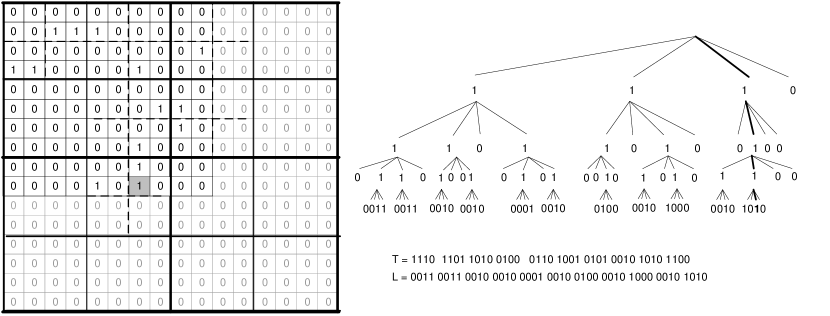
Figure 1: Example of k²-tree for a binary matrix using $k=2$.

This conceptual tree is implemented using two bit arrays: $T$ contains the bits for all the levels of the tree except for the last one, taken in a levelwise traversal of the tree. $L$ stores the bits of the last level of the tree.

The k²-tree allows navigation of the conceptual tree using only the bitmap representations thanks to a basic property: given any internal node in the k²-tree (a position $pos$ in $T$), its k² children will be located at $pos^{\prime}=rank_{1}(T,pos)\times k^{2}$, because each bit set to one adds k² bits to the next level and bits set to zero do not have descendants. If the position exceeds the length of $T$, $L[pos^{\prime}-|T|]$ is used. A rank structure is built over T to provide an efficient $rank_{1}$ operation. All query operations are based on this basic navigation of the conceptual tree.

To access a cell of the matrix, the tree is navigated from the root until a 0 is found or the last level is reached. At each level, the child whose submatrix contains the target cell is selected. If the bit value of that node is 0 we know the cell in the region is a 0, and navigation ends. If the value is 1, we proceed recursively to the appropriate children. For instance, let us suppose we want to retrieve the value of the cell at row 9, column 6 in the matrix of Figure 1. The path to reach that cell has been highlighted in the conceptual k²-tree. To perform this navigation, we would start at the root of the tree (position 0 in $T$). In the first level, we need to access the third child (offset 2), since we are accessing the bottom-left quadrant; hence we access position $2$ in $T$. Since $T[2]=1$, we know we are in an internal node. Its children will begin at position $rank_{1}(T,2)\times k^{2}=12$, where we find the bits 0100. In this level we must access the second child (offset 1), so we check $T[12+1]=T[13]=1$. Again, we are at an internal node, and its children are located at position $rank_{1}(T,13)\times k^{2}=9\times 4=36$. We have reached the third level of the conceptual tree, and we need to access now the second child (offset 1). Again, $T[36+1]=1$, so we compute the position of its children using $p=rank_{1}(T,36)\times 4=80$. Now $p$ is higher than the size of $T$ (40), so the k² bits will be located at position $p-|T|=80-40=40$ in $L$. Finally, in $L$ we find the k² bits 1010, and need to check the third element. We find a 1 in $L$ and return the result.

In addition to the retrieval of a single cell of the matrix, k²-trees can perform other operations efficiently: with some additional calculations, we can modify the basic search to find all the ones in a row/column, or a range [a₁,a₂]-[b₁,b₂]. To do this, at each level of the k²-tree we must access all the children of the current node that overlap the region we are interested in, traversing all the branches of the tree that intersect the region of interest. The cost to perform a general range reporting query in a k²-tree, over a region of size $p\times q$, is bounded by the size of the region and the number $occ$ of results found. The upper bound for the query time is $O(p+q+(occ+1)k\log_{k}s)$, where $s$ is the size of the longest side of the matrix [8, Section 10.2.1].

2.2.1 Improvements

Several enhancements have been proposed to obtain better compression results in the k²-tree (see [29]). The first modification is the use of different values of $k$ in different levels of the k²-tree. By using a bigger $k$ for the first levels and a smaller value for the remaining ones, one can achieve better query times (because the k²-tree’s height is reduced) with good space results. This is called a hybrid k²-tree representation.

Another major improvement proposed over basic k²-trees is the use of a compression method for the bitmap $L$. In this approach, the lowest levels of the k²-tree are grouped, yielding submatrices of size $k^{\prime}\times k^{\prime}$ (for instance, to use $8\times 8$ submatrices as the last level of the tree instead of $2\times 2$). These submatrices are sorted according to their overall frequency and stored in a matrix vocabulary $L^{voc}$. Then, the bitmap $L$ is replaced by a sequence of variable-length codes $L^{seq}$. The variable-length codes are assigned using (s,c)-Dense Codes [30], and $L^{seq}$ is encoded using Direct Access Codes [31] to provide direct access to any entry in the sequence. This variant can reduce significantly the size of the representation while showing similar query times.

3 The dynamic k²-tree: dk²-tree

3.1 Data structures

The conceptual k²-tree is represented, in its static variant, using two bit arrays, $T$ and $L$. In our dynamic version, we represent $T$ and $L$ with two trees, that we call T_tree and L_tree. Our approach to represent the k²-tree using these trees is called dk²-tree. Our trees, T_tree and L_tree, are in fact practical implementations of dynamic bit vectors [32] replacing the static bitmaps $T$ and $L$. The leaves of T_tree and L_tree contain roughly the bits in $T$ and $L$, while the internal nodes provide access to arbitrary positions and also act as a dynamic rank structure.

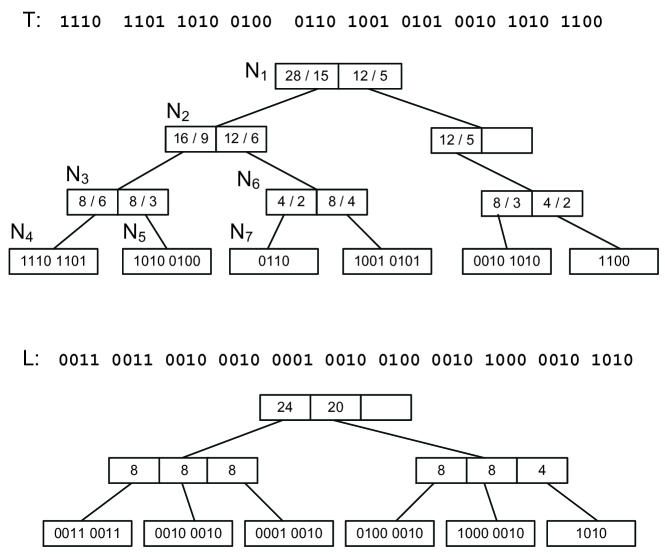
Figure 2: Dynamic k²-tree representation.

Consider a static k²-tree representation (bitmaps $T$ and $L$). To build a dk²-tree representation from it, we partition $T$ and $L$ in blocks of up to $B$ bits. The generated blocks will be the leaves of T_tree and L_tree. The internal nodes of our trees contain a set of entries that allow us to access the leaves for query and update operations. Each entry in T_tree is of the form $\langle b,o,P\rangle$, where $b$ and $o$ are counters and $P$ is a pointer to the corresponding child node. The values $b$ and $o$ in each entry will allow us to efficiently access and perform rank operations in the dynamic bitmaps. If $P$ points to a leaf node, the counters will store the number $b$ of bits stored in the leaf and the number of them that are ones ($o$). If $P$ points to an internal node, $b$ and $o$ will contain the sum of all the $b\mathchar 45\relax$ and $o\mathchar 45\relax$counters in the child node. Internal nodes in L_tree are very similar, but entries only store values $\langle b,P\rangle$, since rank support in $L$ is not needed. Figure 2 shows a dk²-tree representation for the k²-tree of Figure 1. Values of $b\mathchar 45\relax$ and $o\mathchar 45\relax$counters are represented in the nodes, and pointers are visually represented.

The nodes of T_tree and L_tree may in general be partially empty. Each node has a maximum and minimum capacity and may contain any number of bits or entries between those parameters. A $size$ field is added to keep the current size of a node. In leaf nodes, this field contains the number of bits stored in the block. In internal nodes, it stores the number of fixed-size entries used. The tree is completely balanced, and nodes may be split or merged when the contents change. The behavior of T_tree and L_tree on update operations will be explained in more detail in Section 3.3.

3.2 Query algorithms

All the queries supported by k²-trees are based on access and rank operations over the bitmaps $T$ and $L$. As explained before, our tree structures, T_tree and L_tree, are essentially dynamic replacements for the static bitmaps. By providing basic support for these two simple operations in the bitmaps stored by T_tree and L_tree, all the queries supported by static k²-trees can be directly supported by our dk²-tree.

The navigation of a conceptual k²-tree is based on a sequence of access operations, to check the value of a node, followed by possible rank operations to locate its children. The access operation, that is trivial in a static bitmap, is decomposed in our T_tree and L_tree in two steps: first, an operation findLeaf is used to locate the leaf that contains the desired bitmap, and the offset in the leaf node where the bit should be; then, we access the leaf node’s bitmap to retrieve the actual values. This findLeaf operation also computes information about the number of ones up to the beginning of the leaf node, to allow efficient computation of rank operations if necessary.

Two slightly different algorithms are used to access a leaf in T_tree and L_tree, but the essential steps are the same. Starting at the root of T_tree or L_tree, the entries of the current node are checked from left to right, accumulating the values of $b\mathchar 45\relax$ and $o\mathchar 45\relax$counters in two variables, $b_{\mathrm{before}}$ and $o_{\mathrm{before}}$, until we exceed the desired position $p$. The algorithms proceed to the corresponding child node that would contain $p$. When a leaf node is found, the values of $b_{\mathrm{before}}$ and $o_{\mathrm{before}}$ contain the bit count and rank to the left of the node.

Once findLeaf returns the leaf node $N_{\ell}$ that contains the desired position, we can access the desired bit at position $p-b_{\mathrm{before}}$ in the bitmap of the leaf node ($T_{\ell}$). If the bit has value 0, navigation ends. Otherwise, and assuming we are still in the upper levels of the conceptual k²-tree, we would need to locate its children, that will be located at position $\emph{rank}_{1}(T_{tree},p)\times k^{2}$. The rank value is computed as $o_{\mathrm{before}}+rank_{1}(T_{\ell},p-b_{\mathrm{before}})$.

The rank operation in $T_{\ell}$ can still be a costly operation for relatively large node sizes. In order to speed up the local rank operation inside the leaves of T_tree (rankLeaf operation), we add a small rank structure to each leaf of T_tree. This rank structure is simply a set of counters that stores the number of ones in each block of $S_{T}$ bits. $S_{T}$ determines the number of samples that are stored in each leaf and provides a space/time tradeoff for the local rank operation inside the leaves of T_tree. Using this modified leaf structure, $rank_{1}(T_{\ell},p)$ is obtained adding the values of all samples previous to position $p$ and performing a sequential counting operation only from the last sampled position.

3.2.1 Improving access times

An actual query in a k²-tree involves usually a top-down traversal, following a number of branches of the conceptual tree. This top-down traversal actually translates into a set of accesses to the bitmaps $T$ and $L$. These accesses follow a well-defined pattern, starting at the beginning of the bitmap and accessing new positions left to right.

Taking advantage of this property, we propose an alternative strategy to navigate the dk²-tree. In this strategy, to access a position in T_tree or L_tree we start the search from the previously accessed leaf instead of the root node. Instead of a fixed number of internal nodes to be traversed top-down, the new algorithm will first traverse the tree bottom-up until a descendant of the new node is found, and then continue top-down as the original algorithm. This method aims at taking advantage of the access patterns in the k²-tree bitmaps, since many accesses, especially in upper levels, will be located in the same or very close leaf nodes in T_tree.

To be able to start search from a previously accessed leaf node, a new $\mathit{findLeaf}^{*}$ operation must store a small array containing information about the last traversed path. levelData$[$T_tree.depth$]$ is kept, that stores for each level of T_tree, an entry $\langle N,e,s,b,o\rangle$, where $N$ is the T_tree node accessed at that level, $e$ the entry that was traversed, $s$ is the number of bits covered by $N$ and $b$ and $o$ are the values of $b_{\mathrm{before}}$ and $o_{\mathrm{before}}$. A similar array is kept for L_tree, only ignoring the $o$ values in each entry.

The path information from the previous call allows $\mathit{findLeaf}^{*}$ to determine whether the current leaf node contains the new desired position. If it does, the method returns immediately. Otherwise, the parent node is checked recursively until we find an internal node that “covers” the new position. From that point on, the algorithm behaves exactly like the original findLeaf and its top-down traversal.

3.3 Update operations

In addition to the queries supported by static k²-trees, dk²-trees must support update operations over the binary relation. First, relations between existing elements may be created or deleted (changing zeros of the adjacency matrix into ones and vice versa). Additionally, dk²-trees support changes in the base sets of the binary relation (new rows/columns can be added to the binary adjacency matrix, and existing rows/columns can be removed as well).

3.3.1 Changing the contents of the binary matrix

Changes in the binary matrix represented by a k²-tree lead to a set of modifications in the conceptual tree representation, essentially the creation or removal of branches in this conceptual k²-tree. We will describe the changes caused in the conceptual tree and its bitmap representation. Then we will explain how these changes in the bitmaps are implemented over the data structures T_tree and L_tree.

In order to insert a new 1 in a binary matrix represented with a k²-tree, we need to make sure that an appropriate path exists in the conceptual tree that reaches the cell. The insertion procedure begins searching for the cell that has to be inserted, until a 0 is found in the conceptual tree. Two cases may occur:

• If the 0 is found in the last level of the conceptual tree, the 0 is simply replaced by a 1 to mark the new value of the cell and the update is complete.

• If the 0 is found in the upper levels of the conceptual tree, a new path must be created in the conceptual tree until the last level is reached. First, the 0 is replaced with a 1 as in the previous case. Then, groups of k² bits must be added in the lower levels. After replacing the 0 with a 1, a rank operation is performed to compute the position where its children should be located. Then k² 0 bits are added as children, and the one that “covers” the position inserted is set to 1. The procedure continues recursively until it reaches the last level in the conceptual tree.

Notice that there is still a third scenario corresponding to the case where a 1 already exists in the cell to be inserted. However we do not consider it, as in this case the element is already inserted (and the appropriate path is already present as well), hence no change is actually made in the representation. Figure 3 shows an example of insertion in a conceptual tree. At a given level in the conceptual tree a 0 is found and replaced with a 1, and a new path is created adding k² bits to all the following levels. The new branch is highlighted in gray and the changes in the bitmaps of the k²-tree are also highlighted.

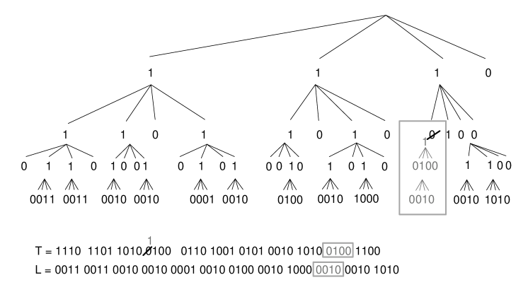
Figure 3: Insert operation in a k²-tree: changes in the conceptual tree.

To change a 1 into a 0 in the binary matrix, we need to set to 0 the bit of the last level that corresponds to the cell. Then, the current branch of the conceptual tree must be checked and updated if necessary. First, we locate the position of the cell to be deleted in the tree. The bit (node) corresponding to that cell is set to 0. After this, we check the $k^{2}-1$ bits corresponding to the siblings of that node. If at least one of the bits is set to 1 the procedure ends. However, if all of them are set to 0, this means that there are no 1s remaining in the current branch: we need to delete the complete group of k² 0 bits, move one level up in the conceptual tree and set the bit corresponding to their parent node to 0. We recursively repeat the same procedure upwards until a group of non-zero k² bits is found.

Summarizing the previous explanation, in order to support insertions and deletions in the conceptual dk²-tree we only need to provide three basic update operations in the dynamic bitmaps T_tree and L_tree: flipping the value of a single bit, adding k² bits at a given position and removing k² bits starting at a given position. For example, Algorithm 1 shows the complete process of insertion of new 1s in the matrix.

Algorithm 1 Insert operation

function insert(tree, r, c)

    $p\leftarrow 0$

    mode $\leftarrow$ Search

    for $l\leftarrow 0$ to tree.nlevels - 1 do

5:       $p\leftarrow\textsc{computeChild}(p,r,c,l)$

       ($N_{\ell}$, $b_{\mathrm{before}}$, $o_{\mathrm{before}}$) $\leftarrow$ findLeaf(T_tree, $p$)

       $T_{\ell}\leftarrow N_{\ell}.data$

       if  mode = Search then

          if $access(T_{\ell},p-b_{\mathrm{before}})=0$ then

10:             $\textsc{flip}(T_{\ell},p-b_{\mathrm{before}})$

             mode $\leftarrow$ Append

          end if

       else

          $\textsc{append4}(T_{\ell},p-b_{\mathrm{before}})$

15:          $\textsc{flip}(T_{\ell},p-b_{\mathrm{before}})$

       end if

       $rank\leftarrow o_{\mathrm{before}}+rank_{1}(T_{\ell},p-b_{\mathrm{before}})$ $\triangleright$ $rank_{1}(tree,p)$

       $p\leftarrow rank\times k^{2}$

    end for

20:    $l\leftarrow tree.nlevels$

    $p\leftarrow p-tree.T_{tree}.length$

    $p\leftarrow\textsc{computeChild}(p,r,c,l)$

    ($N_{\ell}$, $b_{\mathrm{before}}$) $\leftarrow$ findLeaf(L_tree, $p$)

    $T_{\ell}\leftarrow N_{\ell}.data$

25:    if  mode = Search then

       if $access(T_{\ell},p-b_{\mathrm{before}})=0$ then

          $\textsc{flip}(T_{\ell},p-b_{\mathrm{before}})$

          mode $\leftarrow$ Append

       end if

30:    else

       $\textsc{append4}(T_{\ell},p-b_{\mathrm{before}})$

       $\textsc{flip}(T_{\ell},p-b_{\mathrm{before}})$

    end if

end function

To flip a single bit in T_tree or L_tree, we first retrieve the leaf node $N_{\ell}$. The bit is changed in the bitmap of $N_{\ell}$ and its local rank directory is updated (simply adding or subtracting 1 to the value of the appropriate counter). Finally, if we are updating T_tree, the $o$-counters in the entries followed in the path to $N_{\ell}$ must be updated to reflect the change.

To add k² bits at a given position in $N_{\ell}$, the k² bits are inserted in the bitmap of $N_{\ell}$ directly, and the counters in the rank directory of $N_{\ell}$ must be updated accordingly (in this case, all the counters from the position in $N_{\ell}$ where the insertion has been done until the end of $N_{\ell}$ bitmap must be updated, since the bitmap is displaced). After updating $N_{\ell}$, the $b\mathchar 45\relax$ and $o\mathchar 45\relax$counters of its ancestors are also updated accordingly (the $b\mathchar 45\relax$ and $o\mathchar 45\relax$counters are increased by k² and 1 respectively). Notice that we only update the $b\mathchar 45\relax$ and $o\mathchar 45\relax$counters of the entries in the path to $N_{\ell}$ because only those entries are affected by changes in the bitmap of $N_{\ell}$.

When a leaf of T_tree or L_tree reaches its maximum node size we split it in two nodes, always keeping groups of k² sibling bits in the same leaf. This change is propagated to the parent of the leaf node, causing the insertion of a new entry pointing to the new node and updating the $b\mathchar 45\relax$ and $o\mathchar 45\relax$counters accordingly. Eventually, internal nodes may also be split, evenly splitting their entries in two new nodes.

To achieve better space utilization the dk²-tree can store nodes of different maximum sizes. Given a base node size $B$, we allow a number $e$ of partial expansions of the node before splitting it. Hence, T_tree and L_tree may contain nodes of size $B$, $B+\frac{B}{e+1}$, $\cdots$, $B+\frac{(e)B}{e+1}$ (class-0, $\cdots$, class-$e$ nodes). If a node overflows, its contents are reallocated in a node of the next class. If a fully-expanded node overflows, it is split into two class-0 nodes.

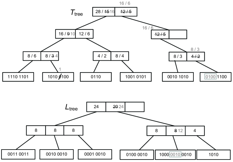
Figure 4: Insert operation in a dk²-tree: changes in the data structures.

3.3.2 Changes in the rows/columns of the adjacency matrix

The dk²-tree also supports the insertion of new rows/columns in the adjacency matrix it represents, as well as deletion of existing rows/columns.

The insertion of new rows/columns to the adjacency matrix is trivial in many cases in the dk²-tree. Note that if the size of the matrix is not a power of $k$ it is virtually expanded to the next power of $k$ to represent it with a k²-tree. Therefore, in a k²-tree we usually have unused rows and columns that can be made available. If the size of the matrix is exactly a power of $k$ we can easily add new unused rows expanding the matrix. To do this, we add a new root node to the conceptual k²-tree: its first child will be the current root and its k²-1 remaining children will be 0. This virtually increases the size of the matrix from $k^{n}\times k^{n}$ to $k^{n+1}\times k^{n+1}$. This operation simply requires the insertion of k² bits 1000 at the beginning of T_tree.

To delete an existing row/column, the procedure is symmetric to the insertion. The last row/column of the matrix can be removed by updating the actual size of the matrix and zeroing out all its cells. Rows/columns at other positions may be deleted logically, by adding these positions to a list of deleted rows and columns after zeroing all their cells. This deleted rows/columns could be reused later when new rows/columns are inserted, by just taking one from the list.

3.4 Analysis

As previously stated in Section 1, dynamic representations of compact data structures are usually affected by a slowdown factor that limits their overall efficiency when compared to a static representation. The static k²-tree is essentially a LOUDS-based cardinal tree, and a dynamic representation of a LOUDS tree has a slowdown factor of $\mathcal{O}(\omega)$ to perform range queries [8, Section 12.5.2]. In the RAM model, we can assume this to mean a slowdown of $\mathcal{O}(\log n)$ for any dynamic representation of a LOUDS tree.

Note that in Section 3.2.1 we described an optimization that takes into account the access pattern in the k²-tree (accesses to the tree are not random when performing queries; they follow a well-defined pattern with many consecutive accesses to close positions). This reduces the overall cost from the original $O(C\log n)$ (where $C$ is the cost of the static representation, described in Section 2.2) to $\mathcal{O}(C\log{\frac{n}{C}})$, improving the result especially for costly queries.

Update operations over LOUDS cardinal trees require $\mathcal{O}(\log_{k}n)$ updates, in blocks of $k$ bits [8, Section 12.4.1]. The time required for an update operation becomes $\mathcal{O}(\omega)$ if $k=\mathcal{O}(\omega^{2})$. As this is a rather permissive value for $k$ in practice, we may consider the update cost over the dynamic representation to be $\mathcal{O}(\log n\log_{k}n)$.

4 Improved compression with a matrix vocabulary

Recall from Section 2.2.1 that the k²-tree space results can be improved using a matrix vocabulary to compress the bitmap $L$. This improvement replaces the plain bitmap $L$ with a sequence of variable-length codes and a matrix vocabulary. In this section we introduce a similar proposal for dk²-trees. In this proposal, the leaves in L_tree will store a sequence of variable-length matrix identifiers encoded using ETDC [22, 23].

Note that the management of a matrix vocabulary is much more complex in the dk²-tree: we should be able to add and remove entries from the vocabulary, as well as efficiently check whether a given matrix already exists in the vocabulary. Also, when L_tree stores a sequence of codewords, the actual number of bits and ones in a leaf is no longer the same as the logical values stored in $b\mathchar 45\relax$ and $o\mathchar 45\relax$counters of its parent entry. This does not affect the tree structure because the actual size of each leaf node is stored in the size field of its header, and this is the value used to determine when to expand or split a leaf, while the values in the counters are still used as before to access the appropriate leaf.

To store the matrix vocabulary we built a simple implementation that stores a hash table $H$ to look up matrices. An array $V$ stores the position in $H$ where each matrix is stored. Finally, we add another array $F$ that stores the frequency of each matrix. An additional list $V^{\mathrm{empty}}$ stores the codewords that are not being currently used.

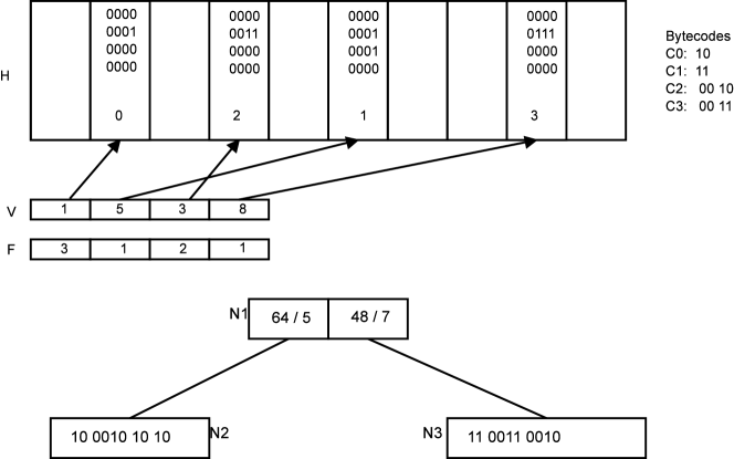
Figure 5: Dynamic vocabulary management: vocabulary (top) and L_tree (bottom).

Figure 5 shows an example with a complete vocabulary representation. The leaves of L_tree (bottom, nodes N2 and N3) store a sequence of variable-length codes represented with ETDC (we consider 2-bit chunks in this simplified example). Notice that the $b\mathchar 45\relax$ and $o\mathchar 45\relax$counters in internal node N1 still refer to the logical size of the leaf: the entry pointing to N2 marks it as containing 64 bits (4 submatrices of size $4\times 4$) and 5 ones. The submatrices are stored in a hash table that contains for each matrix its offset in the vocabulary (that can be easily translated into its ETDC codeword). $V$ points to the entry in $H$ for each vocabulary codeword, and $F$ stores its frequency.

To access a position in L_tree when using a matrix, we obtain a logical offset in the leaf from findLeaf. To retrieve the actual bit, we sequentially traverse the sequence of variable-length codes in the leaf. When we find the code that contains the desired position, we translate the codeword into an array index, and $V$ is used to retrieve the actual matrix in $H$. For example, suppose we want to access position 21 in the example of Figure 5. Our findLeaf operation would take us to node N2, offset 21. To obtain the actual matrix we would traverse the codes in N2, taking into account the actual size of each submatrix (16 bits), so our offset would be at position 5 in the second submatrix. We go over the code 10 and find the second code 0010. To find the actual matrix, we convert this code to an offset (2) and access $V[2]$ to locate the position in $H$ where the matrix is actually stored (3, second non-empty position). Finally, in $H$ we can access bit 5 in the matrix bitmap (0).

The main difference with a static implementation is the need to sequentially traverse the list of variable-length codes. We can reduce the overhead of this sequential traversal adding to the leaves of L_tree a set of samples that store the actual offset in bytes of each $S_{L}$-th codeword. The idea is similar to the sampling used for rank in the leaves of T_tree. With this improvement, to locate a given position we can simply use the samples to locate the previous sampled codeword and then start the search from the sampled position.

4.1 Update operations

Update operations in L_tree, when using a matrix vocabulary, require us to add, remove or modify variable-length codes from the leaves of L_tree. All the update operations start by finding the real location in the node where the variable-length code should be added/removed/modified.

To insert groups of k² bits we need to add a new codeword. The matrix corresponding to the new codeword is looked up in $H$, adding it to the vocabulary if it did not exist and increasing its frequency in $F$. Then, the codeword for the matrix is inserted in the leaf, updating the counters in the node and its ancestors.

To remove groups of k² bits in a leaf node of L_tree a codeword must be removed: we locate the codeword in L_tree, decrease its frequency in $F$ and then we remove the code from the leaf node, updating ancestors accordingly. If the frequency of the codeword reaches 0, the corresponding index in $V$ is added to $V^{\mathrm{empty}}$. When new entries must be added to the vocabulary $V^{\mathrm{empty}}$ will be checked to reuse previous entries and new codes will only be used when $V^{\mathrm{empty}}$ is empty.

To change the value of a bit in L_tree we need to replace existing codewords. First, the matrix for the current codeword is retrieved in $H$ and its frequency is decreased in $F$. We look up the new matrix in $H$. Again, if it already existed, its frequency is increased, and if it is new, it is added to $H$ and its frequency set to 1. Then, the codeword corresponding to the new matrix is inserted in L_tree replacing the old codeword.

Following the example of Figure 5, suppose that we need to set to 1 the bit at position 21 in L_tree. findLeaf would take us to N2, where we have to access the second bytecode 00 10 at offset $5$. This bytecode (C2) corresponds to offset 2 in the ETDC order. We would access $V[2]$ to retrieve the corresponding matrix. The operation would require us to transform the matrix as follows:

$$\begin{array}[]{c}0000\\ 0011\\ 0000\\ 0000\\ \end{array}\longrightarrow\begin{array}[]{c}0000\\ 0111\\ 0000\\ 0000\\ \end{array}$$

The new submatrix already exists, at position 3 in $V$ with frequency 1. Hence, we would need to update the leaf node replacing the old codeword 00 10 with the new codeword C3: 00 11. The vocabulary would also be updated, decreasing the frequency of C2 to 1 and increasing the frequency of C3 to 2.

4.2 Handling changes in the frequency distribution

The compression achieved by the matrix vocabulary depends heavily on the evolution of the matrix frequencies. As the distribution of the submatrices changes the efficiency of the variable-length codes will degrade. The simplest approach to mitigate this problem is to use a precomputed vocabulary from a fraction of the matrix to obtain a reasonably good frequency distribution.

To obtain the best compression results, when the frequency of a submatrix changes too much its codeword should also be changed to obtain the best compression results. This is a process similar to the vocabulary adjustment in dynamic ETDC (DETDC [26, 33]). However, in a dk²-tree, to change the codeword of a submatrix, we must also update all the occurrences of the codeword in the leaves of L_tree. Therefore, a space/time tradeoff exists between vocabulary size and update cost.

To maintain a compression ratio similar to that of static k²-trees we can use simple heuristics to completely rebuild L_tree and the matrix vocabulary: rebuild every $p$ updates or count the number of inversions in $F$. To rebuild L_tree, we must sort the matrices in $H$ according to their actual frequency and compute the new optimal codes for each matrix. Then we have to traverse all the leaves in L_tree from left to right, replacing the old codes with optimal ones. Notice that the replacement can not be executed completely in place, because the globally optimal codes may be worse locally, but the complete process should require only a small amount of additional space. After L_tree is rebuilt, the old vocabulary is simply replaced with the optimal values.

Instead of using the simple heuristics to rebuild the matrix vocabulary, we can keep track of how good the current compression is. To guarantee that the compression of L_tree is never too far from the optimum, we can keep track of the actual optimum vocabulary. To do this, we propose an enhanced vocabulary representation, similar to the adaptive encoding used in DETDC. In our case it would be unfeasible to change the actual vocabulary each time the length of a codeword changes, but we store the optimal vocabulary to know exactly the amount of space that would be gained using an optimal vocabulary.

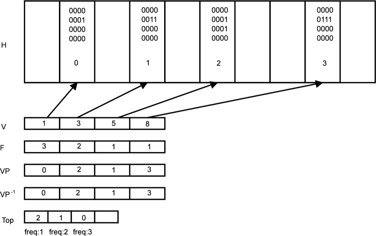
Figure 6: Extended vocabulary to keep track of the optimal codewords.

To this aim we store, in addition to $H$ and $F$, a permutation ${\mathit{VP}}$ between the current vocabulary and the optimal one: ${\mathit{VP}}(i)$ gives the optimal position of the codeword at offset $i$, while ${\mathit{VP}}^{-1}(i)$ gives the current position given the optimal position. This permutation will allow us to keep $V$ and $F$ always sorted in descending order of frequency (that is, according to the optimal vocabulary). Figure 6 shows the data structures required to represent the same vocabulary of Figure 5 using the new method.

In this representation, we obtain the matrix for a codeword as in the previous version; the only difference is that we first obtain the offset of the codeword in the optimal vocabulary and then we use ${\mathit{VP}}^{-1}$ to compute the offset in the current vocabulary. Also, to find the matrix for a given codeword we compute the optimal offset for the codeword using ${\mathit{VP}}$ and then use $V$ to find the position of the matrix.

To keep track of the changes in frequencies, we also build an array, $\mathit{Top}$, that stores, for each different frequency, the position in $V$ of the first codeword with that frequency. The array $\mathit{Top}$ is used to swap codewords when frequencies change, as it is performed in DETDC. If the frequency of a matrix at index $i$ in $V$ changes from $f$ to $f+1$, the new optimum position for it would be the position $\mathit{Top}[f]$. The indexes in $V$, ${\mathit{VP}}$ and $H$ would be updated to reflect the change. The case when the frequency of a matrix decreases from $f$ to $f-1$ is symmetric: we swap the current position of the matrix with $\mathit{Top}[f-1]+1$, updating the corresponding indexes in $F$ and ${\mathit{VP}}$.

The use of the extra data structures allows us to control precisely how much space is being wasted at any moment. This means that we can set a threshold $\mathit{reb_{L_{tree}}}$ and rebuild L_tree when the ratio $\frac{\mathit{size_{cur}}}{\mathit{size_{opt}}}$ surpasses it.

In order to physically store all the data structures required for the dynamic vocabulary, we resort to simple data structures that can be easily updated. $H$ is a simple hash table backed by an array. $V$ and $F$ are extendible arrays. If we want to set the threshold $\mathit{reb_{L_{tree}}}$we need additional data structures for ${\mathit{VP}}$ and $\mathit{Top}$. $\mathit{Top}$ can be implemented using an extendible array and two extendible arrays can store ${\mathit{VP}}$ and its inverse. The goal of these representations is to provide efficient update times (recall that each update operation in the dk²-tree will always lead to a change in L_tree, that will cause at least one frequency change in the vocabulary).

5 Experimental Evaluation

In this section we experimentally test the efficiency of the dk²-tree in order to demonstrate its capabilities to answer simple queries in space and time close to those of the static k²-tree data structure.

First, we will study the different parameters of the dk²-tree and their effect in compression and query efficiency. Then, we will show the efficiency when compared to the equivalent static data structure in the original application domain of k²-trees: Web graph representation. Finally, Section 6 will be devoted to describe the application of dk²-trees to the representation of RDF datasets, where the k²-tree has been already used and dynamic operations are of interest. In this context, we will compare our representation with state-of-the-art alternatives including a similar static approach based on k²-trees.

All the experiments in this article were run on an AMD-Phenom-II X4 955@3.2 GHz, with 8GB DDR2 RAM. The operating system is Ubuntu 12.04. All our code is written in C and compiled with gcc version 4.6.2 with full optimizations enabled.

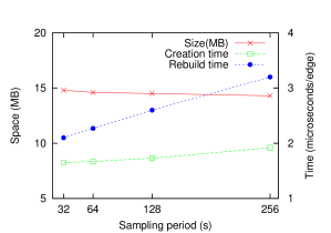
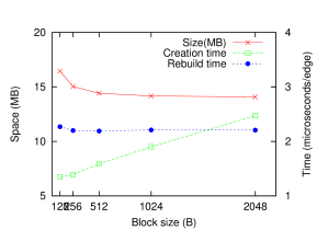
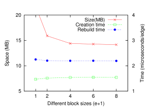
Figure 7: Evolution of space/time results of the dk²-tree changing the parameters $s$, $B$ and $e$.

5.1 Parameter tuning

The main parameters used to settle the efficiency of the dk²-tree are the sampling period $s$ in the leaves of T_tree ($S_{T}$) and L_tree ($S_{L}$), the block size $B$ on the nodes and the number of partial expansions $e$; the value $k^{\prime}$ in the last level is also important when a matrix vocabulary is used for $L$. We will first focus on the effect of the first parameters, and then study the effect of the matrix vocabulary independently.

We use for our experiments a Web graph dataset, eu-2005, a small graph with 19 million edges. The results of parameter tuning are similar for other datasets used in following sections. We do not use a matrix vocabulary in this first example. Figure 7 shows the evolution of the dk²-tree size and the creation and rebuild time depending on each parameter. The dk²-tree size, in MB, is the overall memory used by the data structure. The creation time is the time to build the dk²-tree from a plain representation inserting each edge separately, so it provides an estimation of the average update time of the structure. Finally, the rebuild time is the time to retrieve all the 1s in the adjacency matrix in a single range query covering the complete matrix, and it is shown as a rough estimation of the expected evolution of query times. Both times are shown in microseconds per element inserted/retrieved.

The top-left plot in Figure 7 shows the results obtained for different values of the sampling interval $s$, with fixed $B=512$ bytes and $\#classes=e+1=4$, but the tradeoff is similar for different values. Smaller values of $s$ increase the size of the trees slightly, but a considerable reduction in query time is obtained. Additionally, update operations can also be improved by using smaller values of $s$. Even though blocks with more samples are more costly to update when their contents change, the recomputation of the samples is only performed if the node contents actually change. On the other hand, the rankLeaf operation must always be performed at all the levels of the conceptual tree, and its cost is significantly reduced when using smaller values of $s$. Therefore, a small sampling period can be used to obtain faster access times with only a minor increase in the size of the dk²-tree.

The top-right plot in Figure 7 shows the results for different values of $B$, for fixed $s=128$ bytes and $\#classes=e+1=4$. The block size $B$ provides a clear space/time tradeoff: small values of $B$ yield bigger dk²-trees due to the amount of overhead to store many smaller nodes, while larger values of $B$ make updates become more costly. Query times are not very different depending on $B$ for usual values. In our experiments we will choose values of $B=256$ or $B=512$ to obtain good space results with small penalties in update times.

The bottom plot of Figure 7 shows the evolution with $e$ for fixed $s=128$ and $B=512$. If we use a single block size ($e+1=1$), the node utilization is low and the figure shows poor space results, but even for a relatively small number of block sizes the space results improve fast with only minor changes in the creation and rebuild times.

After measuring the basic parameters of the dk²-tree data structure, we focus on the analysis of the matrix vocabulary variant. We build a dk²-tree for several Web graph datasets with and without a matrix vocabulary and for different values of the parameter $k^{\prime}$. We compare the static and dynamic representations in two different Web graph datasets: the indochina-2004 dataset, with 200 million edges, and the uk-2002 dataset, with 300 million edges. In all cases we built a hybrid variant of the k²-tree or the dk²-tree, with $k=4$ in the first 5 levels of decomposition and $k=2$ in the remaining levels. For the variants with matrix vocabulary, we test the values $k^{\prime}=4$ and $k^{\prime}=8$. In the dk²-tree we choose a block size $B=512$, $e=3$ (4 different block sizes) and $s=128$. The static k²-tree representation uses a sampling factor of 20 for its rank data structures, hence requiring an additional 5% space.

We use in the dk²-tree the most complex version of the matrix vocabulary, that keeps track of the optimum vocabulary and rebuilds the complete vocabulary when the total size is 20% worse than the optimum. Additionally, we set a threshold of 100 KB for the size of L_tree, so that the vocabulary is only checked (and rebuilt if necessary) when L_tree reaches that size. We also consider in the dk²-tree two different scenarios: the space required by the simplest version of the vocabulary (dynamic) and the total space required to keep track of the optimum vocabulary (dynamic-complete).

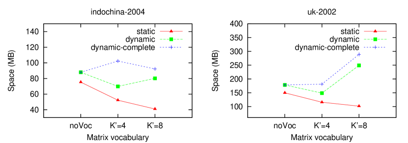
Figure 8: Space utilization of static and dynamic k²-trees with different matrix vocabularies in Web graphs.

Figure 8 shows the evolution of the space utilization for both datasets required by original k²-trees (static) and a dk²-tree (dynamic). Note that the dk²-tree space utilization is always close to that of the static k²-tree when no matrix vocabulary is used ($noVoc$). The space overhead of dk²-trees, around 20%, is mostly due to the space utilization of the nodes of T_tree and L_tree.

Static k²-trees obtain better compression for larger values of $k$’, reaching their best space utilization when $k^{\prime}=8$. On the other hand, the dk²-tree improves its space results only for small $k$’. Note also that the variant that keeps track of the optimum vocabulary ($dynamic-complete$) is always bigger than the simpler approach. In fact, in our experiments the graphs were only rebuilt once, when the size of L_tree reached the threshold, showing that once a small fragment of the adjacency matrix has been built the resulting matrix vocabulary becomes good enough to compress the overall matrix with a relatively small penalty in space. Hence, the size of the additional data structures required to keep track of the optimum vocabulary is higher than the space reduction of the vocabulary itself. Considering these results, a simpler strategy to maintain a “good” matrix vocabulary (such as using a predefined matrix vocabulary extracted from experience or simply rebuilding after $x$ operations) may be the best approach in many domains. On the other hand, the strategy to keep track of the optimum vocabulary could still be of application in domains where the relative size of the matrix vocabulary is expected to be of small size.

5.2 Query and update times

In this section we extend the previous analysis of the dk²-tree measuring the efficiency of our proposal in terms of query and update times.

To measure the query efficiency, we focus on the representation of Web graphs, the original application domain of the static k²-tree. We choose the most usual query in this domain, namely, the successor query that asks for the direct neighbors of a specific node (all the cells with value 1 in a specific row of the adjacency matrix). For each dataset we run successor queries for all the nodes in the dataset and measure the average query times in $\mu$s/query.

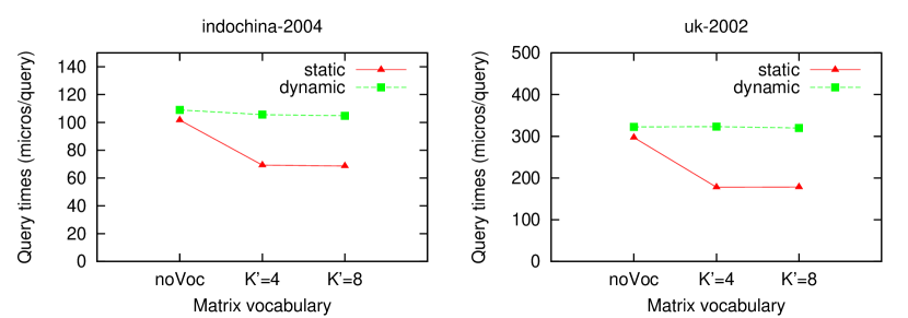
Figure 9: Time to retrieve the successors of a node in a static k²-tree and a dk²-tree. Query times in $\mu$s/query.

As shown in Figure 9, the dk²-tree is always slower than a static representation. Comparing the dk²-tree version that obtained the best space results ($k^{\prime}=4$) with the best static k²-tree version ($k^{\prime}=8$), the dk²-tree is 50-80% slower than the static data structure. This difference in query times is significant, but for specific scenarios where update operations are frequent, the dk²-tree turns out to be a reasonable solution especially if we consider the slowdown that affects any dynamic representation, and the limitations of its static version.

The cost of update operations in the dk²-tree depends on several factors, such as the choice of parameters $B$ and $s$. The characteristics of the dataset also have a great influence in its k²-tree and dk²-tree representation, since the clusterization of 1s lead to a better compression of the data. In the dk²-tree, the clusterization of 1s and the sparsity of the adjacency matrix also affect update times: when new 1s must be inserted and they are far apart from any other existing 1, the insertion operation must insert k² bits in many levels of the conceptual k²-tree, which increases the cost of the operation. Therefore, insertion costs are expected to be higher on average when datasets are very sparse.

To measure this effect of the distance between 1s on update costs, we choose to use synthetic datasets. Since we aim to evaluate the insertion cost depending on the level of the conceptual tree where that insertion is performed, synthetic data allow us to specifically control that without depending on other features of specific real Web graphs that were used instead. We create a set of very sparse synthetic datasets. In them, 1s are inserted every $2^{d}$ rows and $2^{d}$ columns, so that the k²-tree representation has a unary path of length $d$ to each edge. Table 1 shows a summary with the basic information of the datasets. We choose the separation for the different dataset sizes so that all the datasets have the same number of edges (4,194,304).

Dataset	#rows/columns	Separation between 1s ($2^{d}$)	# k2-tree levels
synth_22	4,194,304	2,048 ($d=11$)	22
synth_24	16,777,216	8,192 ($d=13$)	24
synth_26	67,108,864	32,768 ($d=15$)	26

Table 1: Synthetic sparse datasets used to measure insertion costs.

We measure the insertion cost with these datasets, depending on the number of levels $\ell$ that must be created in the conceptual k²-tree to insert the new 1. We compare the insertion costs for $\ell\in[0,10]$. For each dataset and value of $\ell$, we create a set of 200,000 cells of the matrix that require exactly $\ell$ new levels in the conceptual tree. In this experiments we use a simple setup with a single block size. Additionally, we compute the cost to query the new cells over the unmodified synthetic datasets. These queries are an approximation of the insertion cost that is actually due to locating the node of the conceptual k²-tree where we must start the insertion.

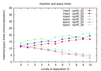
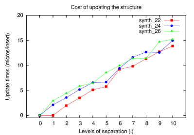
Figure 10: Insertion and query times (left) and estimation of update cost (right) in the dk²-tree varying $\ell$.

Figure 10 (left) shows the evolution of insertion and query times, in $\mu s/edge$, in the different datasets. When $\ell$ is small (new 1s are inserted very close to existing 1s), insertion and query times are almost identical. As $\ell$ increases the insertion cost becomes higher while query times become lower because the first 0 in the conceptual tree (the node where insertion should start) is found in upper levels of the tree. Figure 10 (right) shows an estimation of the actual cost devoted to update the tree depending on $\ell$, and computed by subtracting query times from insertion times. Notice that it is 0 for small $\ell$ and steadily increases with $\ell$.

Our overall results suggest that insertion times in the dk²-tree can be very close to query times if the represented dataset has some properties that are also desirable for compression, particularly the clustering of 1s in the binary matrix. The evolution of insertion times shows that insertions at the upper levels of the tree may be several times more costly than insertions in the lower levels of the tree. However, insertions in the upper levels of the tree should be very infrequent in most of the datasets where a dk²-tree will be used, since compression in k²-trees also degrades when matrices have no clusterization at all.

6 Representation of RDF databases

RDF (Resource Description Framework) [35] has become an increasingly popular language recommended by the W3C for the description of facts in the Web of Data. It follows a graph-based data model, in which the information is represented as a set of triples. Each triple is an edge of a labeled graph, and represents a property of a resource using a subject S (element of interest, or source node), a predicate P (property of the element, or edge label), and an object O (value of the property, or target node). These (S,P,O) triples can be queried using a standard graph-matching language named SPARQL [36]. This language is built on top of triple patterns, that is, RDF triples in which each component may be a variable (variables are preceded, in the pattern, by the symbol $?$): $(S,P,O)$, $(?S,P,O)$, $(?S,?P,O)$, etc. Yet, more complex queries can be created by joining sets of triple patterns.

Many different proposals have appeared in recent years to efficiently store and query RDF datasets. Many of these so called “RDF stores” are based on relational databases, creating specific database structures to store the triple patterns in the RDF data [37, 38]. Other particular solutions rely on specific data structures designed to compactly store the data while allowing efficient query operations [39, 40, 41, 42].

RDF datasets can be built from snapshots of data and therefore stored in static form. However, in many cases new information is continuously appearing and must be incorporated into the dataset to keep it updated. In these cases, a purely static representation of the dataset is unfeasible, since a way to efficiently update the contents in the RDF dataset is needed. Most of the relational approaches for RDF storage can handle update operation. However, specific compact representations usually lack the same flexibility, but still some proposals exist, like X-RDF-3X [43], a dynamic evolution of the existing multi-indexing native solution RDF-3X.

A representation of RDF datasets based on k²-trees, called k²-triples, has been presented in [44]. This representation uses a collection of k²-trees to represent the triples corresponding to each predicate in the RDF dataset. This representation was proved to be very competitive in space and query times with state-of-the-art alternatives. However, this proposal was limited to a static context due to the static nature of k²-trees.

In this section we propose a dynamic representation of RDF datasets based on dk²-trees, that simply replaces static k²-tree representations with a dk²-tree per predicate. We aim to demonstrate that a representation based on the dk²-tree can obtain query times close to the static k²-triples approach, but more importantly that the dk²-tree representation provides the basis to perform update operations on the RDF dataset, which are actually expected operations in real applications.

6.1 Our proposal

Our proposal simply replaces the static k²-tree representation in k²-triples with a dk²-tree per predicate. We consider a partition of the RDF dataset by predicate, and build a dk²-tree for each predicate in the dataset. For each predicate we consider a matrix storing all relations between subjects and objects with that predicate. All matrices will contain the same rows/columns, where subject-objects (elements that appear as both subjects and objects in any triple) will be located together in the first rows/columns of the matrix and the remaining rows (columns) of the matrices will contain the remaining subjects (objects).

Our proposal based on dk²-trees aims to solve the representation of the structural part of an RDF dataset. We assume that additional data structures must be used to store vocabularies of subjects, objects and predicates and map them with rows/columns of the matrices represented by dk²-trees. The creation of a dynamic and efficient dictionary representation to manage large collections of URIs and literal values is a complex problem, since the vocabulary may constitute a large part of the total size of an RDF dataset [45].

As previously stated, the main query operations in RDF datasets are based on triple-pattern matching. These triple patterns can be easily translated into a collection of simple queries in one or more of the k²-trees used to store the complete RDF dataset. Hence, our proposal can directly answer all triple pattern queries: $(S,P,O)$ and $(S,?P,O)$ queries are actually cell retrieval queries (involving one dk²-tree or all the dk²-trees in the collection, respectively), $(S,P,?O)$, $(S,?P,?O)$, $(?S,P,O)$ and $(?S,?P,O)$ are row/column queries and $(?S,P,?O)$ is a full range retrieval query that asks for all the cells in a dk²-tree.

Triple patterns can usually be joined to build more complex queries. Join operations involve matching multiple triple patterns with a common element. For instance, the query $(?S,P_{1},O_{1})\bowtie(?S,P_{2},O_{2})$ represents all the subjects that relate to $O_{1}$ with predicate $P_{1}$ and to $O_{2}$ with predicate $P_{2}$. The join variable is marked with an $?$, and is a common element to both triple patterns. In static k²-triples, three different strategies were proposed to solve triple patterns, and all of them can be also used in our dk²-trees:

• Independent evaluation separates any join operation in two triple pattern queries and a simple merge that intersects the results of both queries. The adaptation to dk²-trees is trivial using the basic operations explained.

• Chain evaluation chains the execution, solving first one of the triple pattern and then restricting the second pattern to the results of the first.

• Interactive evaluation is a more complex operation, in which two k²-trees are traversed simultaneously. The basic elements of this strategy include a synchronized traversal of the conceptual trees. Regardless of the type or complexity of the join operation, the essential steps of interactive evaluation are based on the access to one or more nodes in the conceptual trees of different k²-trees, operations that are directly supported by dk²-trees.

6.1.1 Update operations using dk²-trees

Our proposal is able to answer all the basic queries supported by k²-triples simply replacing static k²-trees by dk²-trees. Next, we will show that update operations in RDF datasets can also be easily supported by our proposal. This is presented as a proof of concept of the applicability of dk²-trees to this domain, even though our proposal focuses only on the representation of the triples.

The most usual update operation in an RDF dataset is probably the insertion of new triples, either one by one or, more frequently, in small collections corresponding to new information retrieved or indexed regularly. The insertion of new triples in an existing RDF database involves several operations in our representation based on dictionary encoding:

• First, the values of the subject, predicate and object of the new triple must be searched in the dictionary, and added if necessary. If all the elements existed in the dictionary the new triple is stored as a new entry in the dk²-tree corresponding to its predicate.

• If the triple corresponds to a new predicate, a new empty dk²-tree can be created to store the new subject-object pair.

• If the subject and/or object are new, we must add a new row/column to all the dk²-trees. As explained before, this operation is usually trivial in dk²-trees. In the worst case, we must increase the size of the matrices, an operation (with a cost comparable to the insertion of a new 1 in the matrix) that must be repeated in all the dk²-trees.

The removal of triples to correct or delete wrong information is a typical update operation in RDF datasets, as well. The possible changes when triples are removed are similar to the insertion case: when triples are removed we may need to simply remove a 1 from a dk²-tree or remove a row/column (marking it as unused) if the subject/objects has no associated triples.

We assume in our representation that subject-object elements are stored together in the top-left region of the matrices, so that join operations do not need to perform additional computations. This allows us to focus on triple pattern queries and ignore the effect of an RDF vocabulary. However, the insertion of triples may cause a subject (object) to become a subject-object, and the deletion of triples may transform a subject-object in just a subject or object. A simple solution to avoid the problem in the dynamic case would be to use a different setup where rows/columns of the matrices would contain all the elements (subjects and objects) instead of storing only subjects in the rows and objects in the columns. It should have small effect in the overall compression, since k²-trees and dk²-trees depend mostly on the number and distribution of the 1s in the matrix than on the matrix size.

In order to follow the original setup with subject-object elements in the first rows/columns of the matrix, when a subject (object) becomes a subject-object we need to move it to the beginning of the matrix. This requires finding all the 1s in the corresponding row (column), allocating a new row and column at the beginning of the matrix and inserting the 1s in the same locations in the new row (column). Note that, even though we only described the ability of dk²-trees to add new rows at the end of the matrix, the process can be trivially extended to add rows at the beginning: given an $n\times n$ matrix, let us assume we place elements starting from the center instead of doing it from the first row/column. With this setup, we can add new subject-object elements from the center towards the top-left corner (thus, expanding the matrix towards the top-left corner), and append new subjects and objects in the usual way (towards the bottom-right corner). That is, we can expand our virtual matrix to add subjects and objects as usual, but also attach new subject-object elements in unused rows/columns in the upper-left section of the matrix. This change has small effect on compression (the elements are still grouped essentially in the same way) and allows us to keep the list of subject-object elements together, hence following the same ordering of the static representation.

6.2 Experimental evaluation on RDF datasets

We compare our proposal based on dk²-trees with the static data structures used in k²-triples and its enhanced version, k²-triples⁺, presented in [44]. The goal of these experiments is to demonstrate the efficiency of dk²-trees in this context, and their ability to act as the basis for a dynamic compact representation of RDF databases. Note that in [44] k²-triples were already proved to be competitive with state-of-the-art representations, both in compression and query times. We will compare the space results and query times of dynamic and static representations to show that dk²-trees can store RDF datasets with a reduced overhead over the space and time requirements of a static representation.

6.2.1 Experimental setup

We experimentally compare our dynamic representation with the equivalent one using static k²-trees. We use a collection of RDF datasets of very different sizes and number of triples, and also include datasets with few and many different predicates. Table 2 shows a summary with some information about the datasets used. The dataset jamendo stores information about Creative Commons licensed music; dblp stores information about computer science publications; geonames stores geographic information; finally, dbpedia is a large dataset that extracts structured information from Wikipedia. As shown in Table 2, the number of predicates is small in all datasets except dbpedia, that is also the largest dataset and will be the best example to measure the scalability of queries with variable predicate.

Collection	#triples	#predicates	#subjects	#objects
jamendo	1,049,639	28	335,926	440,604
dblp	46,597,620	27	2,840,639	19,639,731
geonames	112,235,492	26	8,147,136	41,111,569
dbpedia	232,542,405	39,672	18,425,128	65,200,769

Table 2: RDF datasets used in our experiments.

We build our dynamic representation following the same procedure used for static k²-trees, and a similar setup. Elements that are both subject and object in any triple pattern are grouped in the first rows/columns of the matrices. We use a hybrid k²-tree representation, with $k=4$ in the first 5 levels of decomposition and $k=2$ in the remaining levels. The dk²-tree uses a sampling factor $s=128$ in the leaf blocks, while static k²-trees use a single-level rank implementation that samples every 20 integers (80 bytes). In dk²-trees we use a block size $B=512$ and $e+1=4$ different block sizes.

We test query times in all the approaches for all possible triple patterns (except $(?S,?P,?O)$, that simply retrieves the complete dataset) and some join queries involving just 2 triple patterns. We use the experimental testbed in [44] to directly compare our representation with k²-triples. To test triple patterns, we use a query set including 500 random triple patterns for each dataset and pattern. To test join operations we use query sets including 50 different queries, randomly selected from a larger group of 500 random queries and divided in two groups: 25 have a number of results above the average and 25 have a number of results below the average.

The experimental evaluation of join operations is expected to yield similar comparison results to triple patterns, considering the fact that the implementation of the different strategies to answer join queries is identical in dk²-trees and static k²-trees. As a proof of concept of the applicability of dk²-trees in more complex queries, we will experimentally evaluate dk²-trees, and k²-triples to answer join operations $(?V,P_{1},O_{1})\bowtie(?V,P_{2},O_{2})$ (join 1: only the join variable is undetermined) and $(?V,P_{1},O_{1})\bowtie(?V,?P_{2},O_{2})$ (join 2: one of the predicates is variable). Notice that each join type can lead to 3 different join operations depending on whether the join variable is subject or object in each of the triple patterns: for example, join 1 can be of the form $(?V,P_{1},O_{1})\bowtie(?V,P_{2},O_{2})$ (S-S), $(S_{1},P_{1},?V)\bowtie(?V,P_{2},O_{2})$ (S-O) and $(S_{1},P_{1},?V)\bowtie(S_{2},P_{2},?V)$ (O-O).

6.2.2 Space results

We compare the space requirements of our dynamic representation, based on dk²-trees, with k²-triples and its improvement, k²-triples⁺, in all the studied datasets. We select the k²-tree representations that obtain the best compression results: static k²-trees used in k²-triples and k²-triples⁺ use a matrix vocabulary with $k^{\prime}=8$; dk²-trees do not use a matrix vocabulary. Table 3 shows the total space requirements on the different collections studied.

Collection	k2-triples	k2-triples+	dk2-trees
jamendo	0.74	1.28	1.61
dblp	82.48	99.24	125.34
geonames	152.20	188.63	242.60
dbpedia	931.44	1,178.38	1,151.90

Table 3: Space results for all RDF collections (sizes in MB).

Our dynamic representation is significantly larger than the equivalent static version, k²-triples, in all the datasets. In jamendo, a very small dataset, the dynamic representation requires more than twice the space of k²-triples. However, the overhead required by the dynamic version is smaller in larger datasets and particularly in dbpedia. The dk²-tree with no matrix vocabulary is also able to store the dataset with an overhead below 50% extra in the dblp and geonames datasets. Even though the overhead is significant, the results are still relevant since k²-triples was proved to be several times smaller than other RDF stores like MonetDB and RDF-3X in these datasets (at least 4 times smaller than MonetDB, the second-best approach in space, in all the datasets except dbpedia [44]).

In the dbpedia dataset our proposal has a space overhead around 20% over k²-triples, and becomes smaller than the k²-triples⁺ static representation. This result is mostly due to the characteristics of the dbpedia dataset, that contains many predicates with few triples. The static representations based on k²-triples store a static k²-tree representation for each different predicate, each one containing its own matrix vocabulary. The utilization of a matrix vocabulary does not improve compression in these matrices. However, most of the cost of the representation is in the matrices with many triples, so the matrix vocabulary still obtains the best results overall.

6.2.3 Query times

Triple patterns

We first measure the efficiency of our dynamic proposal in comparison with k²-triples to answer simple queries (triple patterns) in all the studied datasets. The results for all the datasets are shown in different tables: Table 4 shows the results for jamendo; Table 5, the results for dblp; Table 6, for geonames and Table 7, for dbpedia. For each dataset we show the query times of k²-triples, k²-triples⁺ (only in queries with variable predicate) and our equivalent dynamic representation of k²-triples. The last row of each table shows the ratio between our dynamic representation and k²-triples, as an estimation of the relative efficiency of dk²-trees.

	$S,P,O$	$S,P,?O$	$?S,P,O$	$?S,P,?O$	$S,?P,O$	$S,?P,?O$	$?S,?P,O$
k2-triples	1.0	4.6	102.8	6954.1	4.9	39.4	29.3
k2-triples+					1.1	23.6	10.0
Dynamic	1.9	4.8	235.6	12788.5	6.0	34.6	28.4
Ratio	1.88	1.06	2.29	1.84	1.22	0.88	0.97

Table 4: Query times for triple patterns in jamendo. Times in $\mu$s/query.

Solution	$S,P,O$	$S,P,?O$	$?S,P,O$	$?S,P,?O$	$S,?P,O$	$S,?P,?O$	$?S,?P,O$
k2-triples	1.2	79.8	1016.4	771061.6	3.6	1294.1	187.5
k2-triples+					1.7	1102.1	140.8
Dynamic	6.5	92.9	2776.3	1450058.3	14.0	1421.8	247.9
Ratio	5.54	1.16	2.73	1.88	3.87	1.10	1.32

Table 5: Query times for triple patterns in dblp. Times in $\mu$s/query.

Solution	$S,P,O$	$S,P,?O$	$?S,P,O$	$?S,P,?O$	$S,?P,O$	$S,?P,?O$	$?S,?P,O$
k2-triples	1.2	59.4	4588.0	1603677.4	2.9	1192.9	273.7
k2-triples+					1.4	915.9	139.0
Dynamic	9.4	79.6	9544.2	2958262.4	17.9	1514.7	423.5
Ratio	7.71	1.34	2.08	1.84	6.11	1.27	1.55

Table 6: Query times for triple patterns in geonames. Times in $\mu$s/query.

Solution	$S,P,O$	$S,P,?O$	$?S,P,O$	$?S,P,?O$	$S,?P,O$	$S,?P,?O$	$?S,?P,O$
k2-triples	1.1	441.4	10.5	1859.5	7960.3	54497.4	29447.7
k2-triples+					1.4	2216.7	518.3
Dynamic	6.6	561.9	19.1	3870.7	23045.4	83340.2	57051.8
Ratio	6.21	1.27	1.82	2.08	2.90	1.53	1.94

Table 7: Query times for triple patterns in dbpedia. Times in $\mu$s/query.

In most of the datasets and queries, query times of dk²-trees are between 1.2 and 2 times higher than in k²-triples. The results in Table 4 for the dataset jamendo show some anomalies, with the dk²-tree performing faster than a static representation. However, due to the reduced size of the dataset we shall disregard these results and focus on the larger datasets. The results in Table 5, Table 6 and Table 7 show very different query times but the ratios shown in each table are very similar in all three datasets.

Our results evidence that dk²-trees are several times slower than static k²-trees in triple patterns that are implemented with single-cell retrieval queries (i.e. patterns $(S,P,O)$ and $(?S,P,?O)$). Particularly, dk²-trees are 5.5-7.7 times slower than static k²-trees to answer $(S,P,O)$ queries. In this queries, the cost of accessing T_tree and L_tree is very high since a single position is accessed per level of the tree.

In all the remaining patterns, i.e. those that are translated into row/column or full-range queries in one or many k²-trees, dk²-trees are much more competitive with static k²-trees, obtaining query times less than 2 times slower than k²-triples in most cases. These differences are mostly due to the indexed representation used in dk²-trees, that avoids complete traversals of T_tree or L_tree when many close positions are accessed in each query. In all these patterns, multiple positions are accessed at each level of the dk²-tree, in many cases these positions are actually in the same leaf node of T_tree or L_tree, so the additional cost of traversing T_tree or L_tree is greatly diminished.

Let us focus now on the effect of the additional indexes used in k²-triples⁺. In the datasets with few predicates, that are the most usual RDF datasets, k²-triples⁺ is around 1.5-3 times faster than k²-triples, hence up to 10 times faster than dk²-trees in $(S,?P,O)$ queries and up to 3 times faster in the remaining patterns with variable predicate. In the dbpedia dataset, the relative efficiency of k²-triples⁺ is much more significant, reducing query times by several orders of magnitude. This makes dk²-trees much slower than k²-triples⁺ in this dataset to answer patterns with variable predicate.

Join operations

Next we test the efficiency of dk²-trees in comparison with k²-triples to answer join queries. Considering the results obtained with single triple patterns, and in order to better show the relative efficiency of our dynamic representation, we focus on the join operations that are more selective, or require more selective operations in the matrices.

We start our experiments with join 1 ($(?V,P_{1},O_{1})\bowtie(?V,P_{2},O_{2})$). We test the 3 different join strategies applied to this join: i) independent evaluation requires two row/column queries in different k²-trees and an intersection of the results; ii) in chain evaluation, we run a row/column query in the k²-tree corresponding to $P_{1}$ and for each result $v$ obtained we run a single cell retrieval in the k²-tree for $P_{2}$; iii) the interactive evaluation runs two synchronized row/column queries in both k²-trees. We test all the join categories S-O, S-S and O-O and query sets with few results (small) or more results (big).

Figure 11 shows the results for join 1. Given the significant differences in query times between datasets, strategies and even query sets, we normalize all the results so that the query times of static k²-trees are always at the same level. The height of the bar for the static representation will always be 1, and the bar for the dk²-tree representation shows the actual overhead of our dynamic representation. The actual query times in the static representation are also displayed, in ms/query.

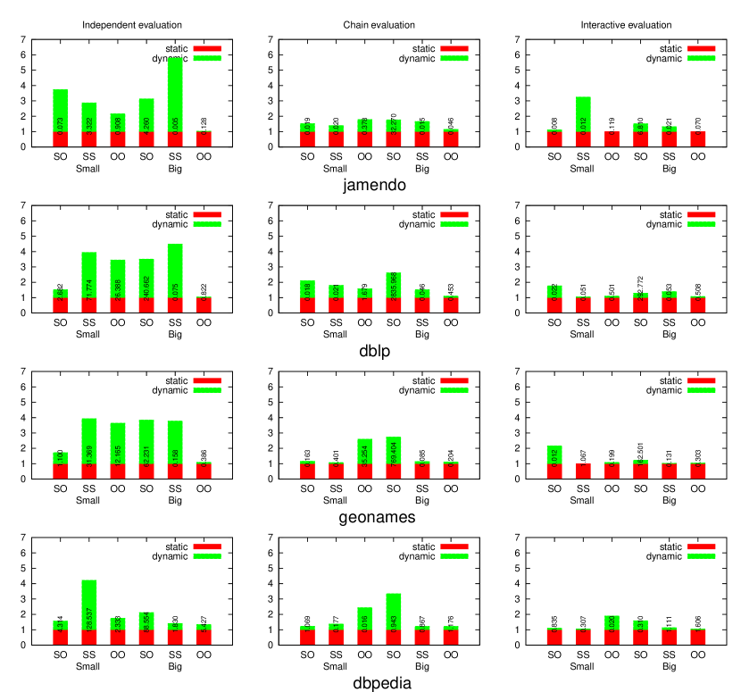
Figure 11: Comparison of static and dynamic query times in join 1 in all the studied datasets and query types. Results are normalized by static query times. Query times of the static representation are shown in ms/query.

Results show that dk²-trees are very competitive with k²-triples in most of the datasets and strategies: independent evaluation (left plots of Figure 11) yields the worst results for dk²-trees, that are 3-4 times slower than k²-triples in most of the query sets, except on the larger dataset dbpedia where our solution is on average less than 2 times slower than static k²-trees. In chain evaluation dk²-trees are less than 2 times slower than a static representation in most of the datasets and query sets. Finally, if we use the interactive evaluation strategy dk²-trees are able to obtain query times very close to static k²-trees in most of the cases.

Averaging the results in all the datasets and query sets for each evaluation strategy, dk²-trees are 3.5 times slower than static k²-trees in the independent evaluation strategy, 2.6 times slower using the chain evaluation strategy and only 27% slower using the interactive evaluation strategy. Even though the results vary significantly between datasets and query sets, the overall results show that dk²-trees are able to support the query operation with a reasonable overhead in space and query times.

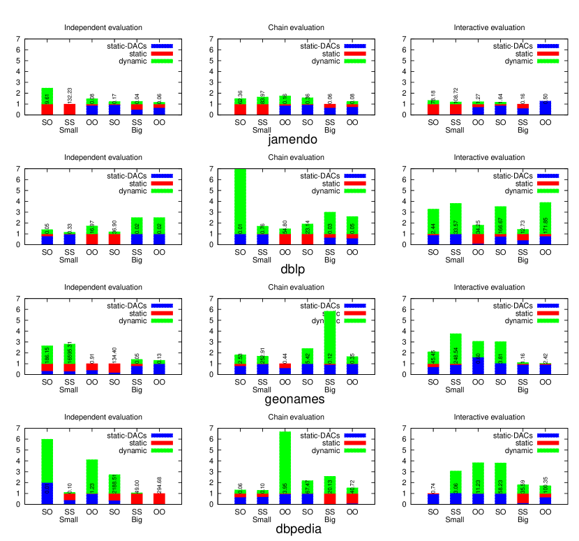
Figure 12: Comparison of static and dynamic query times in join 2 in all the studied datasets and query types. Results are normalized by query times of k²-triples. Query times of the static representation are shown in ms/query.

Join queries with variable predicate

Next we analyze our proposal in join operations with variable predicates. We compare dk²-trees with static k²-triples and k²-triples⁺ (static-DACs) to answer the join 2 ($(?V,P_{1},O_{1})\bowtie(?V,?P_{2},O_{2})$), that involves a variable predicate.

The results are shown in Figure 12. Bar heights are also normalized by the static query times in these graphs. Again, we obtain diverse results in the comparison depending on the dataset, the evaluation strategy and the query set. In spite of the varying results, dk²-trees show again an overhead in query time limited by a small factor: our dynamic representation is between 1.5 and 3 times slower than k²-triples.

If we compare dk²-trees with the best static representation, that is now k²-triples⁺, the overhead required by the dynamic representation becomes larger. Notice that in Figure 12 there are some query sets for which the query times of k²-triples⁺ (static-DACs) are so much lower than k²-triples that the result for k²-triples⁺ is not even visible in the plot. This is consistent with the results obtained in triple patterns, where the use of S-P and O-P indexes in k²-triples⁺ resulted in a major improvement. However, in many cases the improvement obtained by k²-triples⁺ is not so significant and dk²-trees are still reasonably close in query times.

7 Conclusions

The compact representation of static binary relations can be useful in many contexts, but in many application areas relations may be subject to frequent changes. We have introduced the dk²-tree, a representation of binary relations with support for update operations. The dk²-tree is an evolution of the k²-tree, an inherently static data structure that obtained great compression and query times in different types of binary relations. Our dynamic representation is able to obtain good compression and query times, relatively close to those of static k²-trees, and provides at the same time support for the most usual update operations: insertion and deletion of pairs in the binary relation, and also changes in the base sets A and B of the relation.

Our experimental evaluation shows that the dk²-tree, even though it has a significant overhead compared with the static representation, is able to obtain results close enough to those of the static representation to be competitive in areas where the original static representation was already efficient. In particular, we demonstrate that our representation obtains compression results close to a static data structure in Web graphs, and we study the overhead required in the representation of RDF graphs. Our representation performs in general at the same order of magnitude than static k²-trees in this domain, where state-of-the-art alternatives are orders of magnitude larger or slower. Additionally, in many operations and datasets the overhead required by our representation becomes small enough (around 20% space or time overhead in different cases) to be a good representation even in a context of dynamic binary relations with low rate of changes.

References

- [1] N. R. Brisaboa, G. de Bernardo, G. Navarro, Compressed dynamic binary relations, in: Proc. Data Compression Conference (DCC), 2012, pp. 52–61.
- [2] D. J. Abadi, A. Marcus, S. R. Madden, K. Hollenbach, Scalable Semantic Web data management using vertical partitioning, in: Proc. 33rd International Conference on Very Large Data Bases (VLDB), 2007, pp. 411–422.
- [3] J. Barbay, F. Claude, G. Navarro, Compact rich-functional binary relation representations, in: Proc. 9th Latin American Theoretical Informatics Symposium (LATIN), 2010, pp. 170–183.
- [4] P. Boldi, S. Vigna, The WebGraph Framework I: Compression techniques, in: Proc. 12th International World Wide Web Conference (WWW), ACM Press, 2003, pp. 595–601.
- [5] N. R. Brisaboa, S. Ladra, G. Navarro, k2-Trees for compact Web graph representation, in: Proc. 16th International Symposium on String Processing and Information Retrieval (SPIRE), 2009, pp. 18–30.
- [6] F. Claude, S. Ladra, Practical representations for web and social graphs, in: Proc. 20th ACM Conference on Information and Knowledge Management (CIKM), 2011, pp. 1185–1190.
- [7] S. Álvarez-García, N. R. Brisaboa, J. D. Fernández, M. A. Martínez-Prieto, Compressed k2-Triples for full-in-memory RDF engines, in: Proc. 17th Americas Conference on Information Systems (AMCIS), 2011.
- [8] G. Navarro, Compact Data Structures – A practical approach, Cambridge University Press, 2016, iSBN 978-1-107-15238-0. 570 pages.
- [9] T. Käfer, A. Abdelrahman, J. Umbrich, P. O’Byrne, A. Hogan, Observing Linked Data Dynamics, in: Proc. 12th International Semantic Web Conference (ISWC), 2013, pp. 213–227.
- [10] G. Jacobson, Succinct static data structures, Ph.D. thesis, Carnegie Mellon University, Pittsburgh, PA, USA (1989).
- [11] G. Navarro, V. Mäkinen, Compressed full-text indexes, ACM Computing Surveys 39 (1) (2007) art. 2.
- [12] D. Clark, Compact pat trees, Ph.D. thesis, University of Waterloo, Ontario, Canadá (1996).
- [13] J. I. Munro, Tables, in: Proc. 16th Conference of Foundations of Software Technology and Theoretical Computer Science (FSTTCS), 1996, pp. 37–42.
- [14] R. Pagh, Low redundancy in static dictionaries with o(1) worst case lookup time, in: Proc. 26th International Colloquium on Automata, Languages and Programming (ICALP), 1999, pp. 595–604.
- [15] R. Raman, V. Raman, S. Rao, Succinct indexable dictionaries with applications to encoding -ary trees and multisets, in: Proc. 13th ACM-SIAM Symposium on Discrete Algorithms (SODA), 2002, pp. 233–242.
- [16] D. Okanohara, K. Sadakane, Practical entropy-compressed rank/select dictionary, in: Proc. 9th Workshop on Algorithm Engineering and Experiments (ALENEX), 2007.
- [17] K. Sadakane, New text indexing functionalities of the compressed suffix arrays, Journal of Algorithms 48 (2) (2003) 294–313.
- [18] R. Grossi, A. Gupta, J. S. Vitter, When indexing equals compression: experiments with compressing suffix arrays and applications, in: Proc. 15th ACM-SIAM Symposium on Discrete Algorithms (SODA), 2004, pp. 636–645.
- [19] D. K. Blandford, G. E. Blelloch, Compact representations of ordered sets, in: Proc. 15th ACM-SIAM Symposium on Discrete Algorithms (SODA), 2004, pp. 11–19.
- [20] A. Gupta, W.-K. Hon, R. Shah, J. S. Vitter, Compressed data structures: Dictionaries and data-aware measures, in: Proc. 16th Data Compression Conference (DCC), 2006, pp. 213–222.
- [21] V. Mäkinen, G. Navarro, Rank and select revisited and extended, Theoretical Computer Science 387 (3) (2007) 332–347.
- [22] N. R. Brisaboa, E. L. Iglesias, G. Navarro, J. R. Paramá, An efficient compression code for text databases, in: Proc. 25th European Conference on IR Research (ECIR), 2003, pp. 468–481.
- [23] N. R. Brisaboa, A. Fariña, G. Navarro, J. R. Paramá, Lightweight natural language text compression, Information Retrieval 10 (1) (2007) 1–33.
- [24] E. Silva de Moura, G. Navarro, N. Ziviani, R. Baeza-Yates, Fast and flexible word searching on compressed text, ACM Transactions on Information Systems 18 (2) (2000) 113–139.
- [25] D. Huffman, A method for the construction of minimum-redundancy codes, Proceedings of the Institute of Radio Engineers 40 (9) (1952) 1098–1101.
- [26] N. R. Brisaboa, A. Fariña, G. Navarro, J. R. Paramá, Efficiently decodable and searchable natural language adaptive compression, in: Proc. 28th ACM SIGIR Conference on Research and Development in Information Retrieval, 2005, pp. 234–241.
- [27] H. Samet, The quadtree and related hierarchical data structures, ACM Comput. Surv. 16 (2) (1984) 187–260.
- [28] N. R. Brisaboa, S. Ladra, G. Navarro, Compact representation of Web graphs with extended functionality, Information Systems 39 (2014) 152 – 174.
- [29] S. Ladra, Algorithms and compressed data structures for information retrieval, Ph.D. thesis, University of A Coruña (2011).
- [30] N. R. Brisaboa, A. Fariña, G. Navarro, J. Paramá, Lightweight natural language text compression, Information Retrieval 10 (2007) 1–33.
- [31] N. R. Brisaboa, S. Ladra, G. Navarro, Directly addressable variable-length codes, in: Proc. 16th International Symposium on String Processing and Information Retrieval (SPIRE), 2009, pp. 122–130.
- [32] R. Raman, V. Raman, S. S. Rao, Succinct dynamic data structures, in: Proc. 7th International Workshop on Algorithms and Data Structures (WADS), 2001, pp. 426–437.
- [33] N. R. Brisaboa, A. Fariña, G. Navarro, J. Paramá, Dynamic lightweight text compression, ACM Transactions on Information Systems (TOIS) 28 (3) (2010) 10:1–10:32.
- [34] P. Boldi, B. Codenotti, M. Santini, S. Vigna, UbiCrawler: A scalable fully distributed web crawler, Software: Practice and Experience (SPE) 34 (8) (2004) 711–726.
- [35] F. Manola, E. Miller, RDF Primer, W3C Recomm., 2004, www.w3.org/TR/rdf-primer/.
- [36] S. Harris, A. Seaborne, SPARQL 1.1 Query Language, W3C Recomm., 2013, http://www.w3.org/TR/sparql11-query/.
- [37] D. J. Abadi, A. Marcus, S. R. Madden, K. Hollenbach, Sw-store: a vertically partitioned DBMS for Semantic Web data management, The International Journal on Very Large Data Bases 18 (2) (2009) 385–406.
- [38] L. Sidirourgos, R. Goncalves, M. Kersten, N. Nes, S. Manegold, Column-store support for RDF data management: not all swans are white, Proc. VLDB Endowment 1 (2) (2008) 1553–1563.
- [39] T. Neumann, G. Weikum, The RDF-3X engine for scalable management of RDF data, The VLDB Journal 19 (1) (2010) 91–113.
- [40] J. D. Fernández, M. A. Martínez-Prieto, C. Gutiérrez, A. Polleres, M. Arias, Binary RDF representation for publication and exchange (HDT), Web Semantics: Science, Services and Agents on the World Wide Web 19 (2013) 22 – 41.
- [41] J. Urbani, J. Maassen, N. Drost, F. Seinstra, H. Bal, Scalable RDF data compression with MapReduce, Concurrency and Computation: Practice and Experience 25 (1).
- [42] J. Urbani, S. Dutta, S. Gurajada, G. Weikum, KOGNAC: efficient encoding of large knowledge graphs, CoRR abs/1604.04795, http://arxiv.org/abs/1604.04795.
- [43] T. Neumann, G. Weikum, x-rdf-3x: Fast querying, high update rates, and consistency for rdf databases, Proc. VLDB Endowment 3 (1-2) (2010) 256–263.
- [44] S. Álvarez-García, N. R. Brisaboa, J. D. Fernández, M. A. Martínez-Prieto, G. Navarro, Compressed vertical partitioning for efficient RDF management, Knowledge and Information Systems 44 (2) (2015) 439–474.
- [45] M. A. Martínez-Prieto, J. D. Fernández, R. Cánovas, Compression of RDF dictionaries, in: Proc. 27th Annual ACM Symposium on Applied Computing (SAC), 2012, pp. 340–347.