Efficient Enumeration of Induced Matchings in a Graph without Cycles with Length Four

Abstract

We address the induced matching enumeration problem. An edge set $M$ is an induced matching of a graph $G=(V,E)$. The enumeration of matchings are widely studied in literature, but the induced matching has not been paid much attention. A straightforward algorithm takes $O\left(\left|V\right|\right)$ time for each solution, that is coming from the time to generate a subproblem. We investigated local structures that enables us to generate subproblems in short time, and proved that the time complexity will be $O\left(1\right)$ if the input graph is $C_{4}$-free. A $C_{4}$-free graph is a graph any whose subgraph is not a cycle of length four. Finally, we show the fixed parameter tractability of counting induced matchings for graphs with bounded tree-width and planar graphs.

1 Introduction

An enumeration problem is to output all solutions to a given problem without duplication. Enumeration problems and their algorithms have been continuously studied in literature, and recently the studies have got more active from the expansion of the applications, such as data mining, network analysis and computational proofs in mathematics. According to the increase of the activity, several problems that solved in the past were revisited such as paths, cycles, and trees, and several structures began to be studied [7, 9, 20, 21]. In this paper, we also revisit an old fashioned problem of enumerating matchings, but consider its induced version that has not been paid attention much.

The efficiency of enumeration algorithm is often evaluated by output-polynomiality [22]. An algorithm is said to be output-polynomial time if its total running time is bounded by $poly(N,M)$, where $N$ is the input size, $M$ is the output size and $poly(N,M)$ is a polynomial function on $N$ and $M$. The delay of an enumeration algorithm is the maximum computation time between the output solution and the next solution and time after the last solution until the termination of the algorithm. An algorithm is polynomial delay if its delay is bounded by polynomial in $N$. In particular, we say an algorithm is said to runs in $O(poly(N))$ time for each if the algorithm runs in time linear in $Mpoly(N)$.

In this paper, we consider the enumeration problem for induced matchings in the given graph (abbreviated as EIM). An induced matching of a graph is an edge set such that the endpoints of any two edges in the set are not adjacent to each other, i.e., the graph induced by the endpoints of the edge set forms a matching. Uno [21] showed that matchings can be enumerated in a general graph in constant amortized time by using amortization technique, called Push out, to distribute the cost of each iteration to many descendants. We can also consider a straightforward binary partition algorithm (branch and bound algorithm) for induced matching enumeration that runs in $O\left(\Delta^{2}\right)$ time per solution, where $\Delta$ is the maximum degree in an input graph. The structure of the recursion is quite different from the ordinal matching enumeration, thus a direct application of the technique described in  [21] does not work. The push out technique and the other amortization require some conditions, but it is not easy to develop algorithms satisfying the conditions. The existence of more efficient algorithms is still open.

In this kind of low-degree polynomial time enumeration algorithm, the most time consuming part is often typically the generation of the child problems. Particularly, we spend much time when the local structure of the problem is complicated around the pivot vertex or edge, that is to be fixed or to be removed from the problem. If the structure is simple, the child problem generation can be done in short time. For example, if the graph is a tree, there is no cycle around a vertex, thus we do not have to think about unification of multiple edges when we shrink an edge. In this paper, we consider $C_{4}$-free graphs, and propose an algorithm runs in constant time for each, where $C_{4}$-free graphs are graphs that have no cycles of length equal to four. In an ordinal binary partition algorithm for induced matching enumeration, we choose an edge $e$ and enumerate induced matchings including $e$. This is done by enumerating all induced matching included the graph obtained by removing $e$, edges adjacent to $e$, and edges adjacent to edges adjacent to $e$. This takes $O\left(\Delta^{2}\right)$ time and this is the bottle neck of the algorithm. We investigated the $C_{4}$-free graphs, and could find that the structural property of $C_{4}$-free graphs makes the process of generating the subproblems light. We introduced new way of branching the problem, so that in each iteration we select a vertex $v$ with the maximum degree, and partition the problem into $\Delta$ subproblems. The property together with this branching method lighten the computation of subproblems, and the computation time of an iteration is bounded by the number of its descendants. This enables us to use amortization analysis, and can obtain the result.

The organization of the paper is as follows. We show in Sec. 3 that induced matchings are enumerable in constant amortized time per solution for $C_{4}$-free graphs. In Sec. 4, we show that counting all induced matchings can be solvable in FPT linear time for graphs with bounded degree, bounded tree-width, and planar graphs by using the results of [11, 1]. These results seem to show for the first time the complexities of counting and enumeration problems for induced matchings.

Table 1: Summary of our results and related work. This table shows the complexity of path, cycle, matching, and induced matching for each problems. In each cell, we list the complexities of ordinary problem first and parameterized problems next, where the parameter $k$ is included in input in all non-parameterized problems (*), the problem is in FPT for graphs with bounded degree, bounded tree-width, girth at least $6$, line graphs, and planar graphs (^∗∗), the counting problem for $k$-induced matchings is FPT linear for graphs with bounded degree, bounded tree-width, and planar graphs parameterized with an implicit parameter determined by the class (^∗∗∗), the complexity of an enumeration problem shows its amortized complexity per solution.

	decision problem	counting problem	enumeration problem
$k$-path	NP-complete [12]∗	#P-complete [24]∗	Polynomial [18]∗
	FPT [8]	#W[1]-complete [10]
$k$-cycle	NP-complete [12]∗	#P-complete [24]∗	Polynomial [9]∗
	FPT [6]	#W[1]-complete [10]
$k$-matching	P [7]∗	#P-complete [23]∗	$O\left(1\right)$ [21]∗
		#W[1]-complete [4]
$k$-induced matching	NP-complete [19]∗	Unknown	$O\left(1\right)$ for boudned- degree [Ours]∗
	W[1]-complete [16] FPT∗∗ [16]	FPT linear∗∗∗ for bounded tree-width and planar [Ours]	$O\left(1\right)$ for $C_{4}$-free [Ours]∗

1.1 Related works

In Table 1, we show the summary of related work and our results on decision, counting, and enumeration problems for small subgraphs in a graph. The decision problem for matching (maximum matching, MM) has been extensively studied for more than 50 years [7, 14]. The decision problem can be solved in polynomial time for matchings (See [7, 14]), while the problem (MIM) for induced matchings is known to be NP-complete [19]. The latter is still NP-hard for graphs with bounded degree, bipartite graphs, $C_{4}$-free, line graphs, and planar graphs [3, 2, 15]. MIM can be solved in polynomial time for restricted graph classes: interval, chordal, weakly chordal, circular-arc, trapezoid, and co-comparability graphs [2, 13].

In general, counting of matchings is computational hard. In particular, the counting of matchings is #P-complete (Valiant [24]), while it is #W[1]-complete parameterized with the size $k$ of a matching in a bipartite graph (Curticapean and Marx [4]). For enumeration, Uno [21] showed that matchings can be enumerated in constant amortized time per solution. To the best of our knowledge, there are almost no known results for counting and enumeration of induced matchings.

In this paper, we study the complexity of enumeration problems for graphs without cycles of length $4$. Since any graph with girth at least $5$ has no $C_{4}$, our algorithm also works for such graphs with large girth, where the girth of a graph is the length of a shortest cycle in the graph. Recently, there are a few results showing an interesting interplay between induced matchings and graphs with large girth as follows. Raman and Saurabh [17] demonstrated that several fixed parameter intractable problems, such as dominating sets, fall in FPT when input graphs have large girth. As a most closely related result, Moser and Sikdar [16] show that the $W[1]$-hard decision problem for induced matchings becomes in FPT for graphs with bounded degree and with girth $6$ or more.

2 Preliminary

In this paper, for disjoint set $A$ and $B$, we define disjoint union of $A$ and $B$ by $A\sqcup B$. If it is clearly understood, we denote $V(G)=V$ and $E(G)=E$.

Let $G=(V,E)$ be an undirected graph with vertex set $V$ and edge set $E\subseteq V\times V$. In this paper, we assume that graphs have no self-loops or parallel edges. An edge $e$ with vertex $u$ and $v$ is denoted by $e=\{u,v\}$. Two vertices $u,v\in V$ are adjacent if there is an edge $\{u,v\}$ in $E$. We say $u$ is a neighbor of $v$ if $u\in N_{G}(v)$. Similarly, two edges $e,f\in E$ are adjacent if $e$ and $f$ share the same vertex. Let $N_{G}(u)$ be the set of neighbors of $u$ in $G$ and $N_{G}[u]=N_{G}(u)\cup\{u\}$ be the set of closed neighbor of $u$. Let $d_{G}(u)=\left|N_{G}(u)\right|$ be the degree of $u$ in $G$. $\Delta(G)=\max_{x\in V}d(x)$ denotes the maximum degree of $G$. For any vertex subset $V^{\prime}\subseteq V$, we say $G[V^{\prime}]=(V^{\prime},E[V^{\prime}])$ an induced subgraph, where $E[V^{\prime}]=\{\{u,v\}\in E(G)\mid u,v\in V^{\prime}\}$. Since $G[V^{\prime}]$ is uniquely determined by $V^{\prime}$, we identify $V^{\prime}$ with $G[V^{\prime}]$. We denote by $G\setminus\{e\}=(V,E\setminus\{e\})$ and $G\setminus\{v\}=G[V\setminus\{v\}]$. For simplicity, we denote by $v\in G$ and $e\in G$ if $v\in V$ and $e\in E$, respectively.

An alternating sequence $\pi=(v_{1},e_{1},v_{2},\dots,v_{k-1},e_{k},v_{k})$ of vertices and edges is a path if each edge and vertex in $\pi$ appears at most once. We also call $\pi$ an $v_{0}$-$v_{n}$ path. Then, An alternating sequence $C=(v_{1},e_{1},v_{2},\dots,v_{k-1},e_{k},v_{k})$ of vertices and edges is a cycle if $(v_{1},e_{1},v_{2},\dots,v_{k-1})$ is a $v_{0}$-$v_{k-1}$ path and $v_{k}=v_{1}$. The length of a path and a cycle is defined by the number of its edges. Let $G$ be $C_{k}$-free graph if $G$ has no cycle with length $k$ as a subgraph. For example, if $G$ has no $4$-cycles then $G$ is a $C_{4}$-free graph.

For any vertices $u,v\in V$, the distance between $u$ and $v$ is defined by the length of a shortest $u$-$v$ path. The distance between edge $e$ and $f$ is defined by the length of a shortest path, i.e., $dist_{G}(e,f)=\min\{dist_{G}(u,v)\mid u\in e,v\in f\}$. Similarly, the distance between vertex $v$ and edge $e$ is defined by $dist_{G}(v,e)=\min\{dist_{G}(u,v)\mid u\in e\}$.

A matching in a graph $G=(V,E)$ is an edge subset $M\subseteq E$ of $G$, if any pair of edges in $M$ does not share their endpoints. An induced matching in a graph $G=(V,E)$ is a matching $M\subseteq E$ whose vertex set induces $M$ itself. In other words, an edge set $M$ is an induced matching if and only if $dist_{G}(e,e^{\prime})\geq 2$ for any distinct edges $e,e^{\prime}\in M$, i.e., there is no edge $f$ in $G$ connecting $e$ and $e^{\prime}$. In figure 1, we show an example of an induced matching.

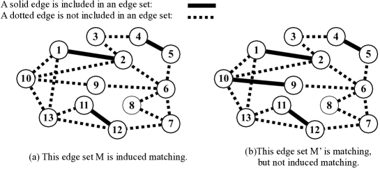
Figure 1: An edge set $M$ in (a) is an induced matching, because all distinct two edges $e,f\in M$ hold $dist_{G}(e,f)\geq 2$. An edge set $M^{\prime}$ in (b) is not an induced matching, because edge $e=\{9,10\}$ and $f=\{1,2\}$ do not hold $dist_{G}(e,f)\geq 2$.

Now, we define the induced matching enumeration problem as follows;

Problem 1 (The induced matching enumeration problem).

Enumerate all induced matching in a given graph $G$ without duplicates.

3 Enumeration of Induced Matchings for $C_{4}$-free Graphs

3.1 Binary partition

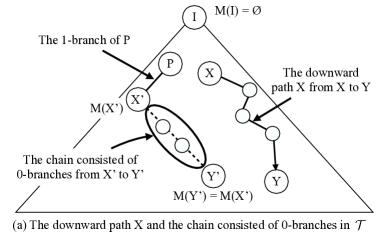
Figure 2: The solid line from $X$ to $Y$ represents a downward path. Consequently, $X\preceq Y$ holds. The dotted line represents a chain consisting of $0$-branches. $X^{\prime}$ is a top of the chain since $X^{\prime}$ is a $1$-child of $P$. $Y^{\prime}$ is a bottom of the chain since $Y^{\prime}$ does not have a child.

A binary partition method is an algorithm which enumerates all solutions by dividing a search space into two disjoint search spaces recursively. We call a dividing step an iteration. Let $G$, $\mathcal{M}(G)$, and $I$ be an input graph, the set of solutions for $G$, and an iteration of the algorithm, respectively. Let $\mathcal{S}(I)$ be the set of solutions included in a search space of $I$. In the initial state, $\mathcal{S}(I)=\mathcal{M}(G)$ holds. At the initial iteration, the algorithm selects an edge $e$ in $G$ such that $e$ satisfies $\left|\mathcal{S}_{0}(I)\right|\geq 1$ and $\left|\mathcal{S}_{1}(I)\right|\geq 1$ where $S_{0}(I)=\{M\in S(I)\mid e\notin M\}$ and $S_{1}(I)=\{M\in S(I)\mid e\in M\}$. Note that $\mathcal{S}(I)=\mathcal{S}_{0}(I)\sqcup\mathcal{S}_{1}(I)$ holds. $\mathcal{A}$ recursively applies this procedure until all edges are selected.

Next, we introduce a binary enumeration tree $\mathcal{T}(\mathcal{I})=\mathcal{T}=(\mathcal{V},\mathcal{E})$, for an input $\mathcal{I}$. Here, $\mathcal{V}$ is the set of iterations of $\mathcal{A}$ for $\mathcal{I}$ and $\mathcal{E}$ is a subset of $\mathcal{V}\times\mathcal{V}$. For any iteration $X$, we define the edge set $E_{X}$ as follows: $E_{X}=\bigcap_{M\in\mathcal{S}(X)}M$. For any iterations $X$ and $Y$, $Y$ is a child of $X$ if $E_{Y}\subset E_{X}$ and $\left|E_{X}\setminus E_{Y}\right|=1$ hold. We call $X$ is the parent of $Y$. For any iteration $X$, we define iterations $X.1$ and $X.0$ with the set of solutions $\mathcal{S}_{1}(X)$ and $\mathcal{S}_{0}(X)$, respectively. That is, $X.1$ and $X.0$ are the children of $X$. In particular, $X.1$ is the $1$-child of $X$, and $X.0$ is the $0$-child of $X$. In addition, we call edges $e=\{X,X.0\}$ and $f=\{X,X.1\}$ in $\mathcal{E}$ a $0$-branch and a $1$-branch, respectively. In the binary enumeration tree $\mathcal{T}$ for $\mathcal{I}$, we call an iteration with children an internal iteration, and an iteration without children a leaf iteration. Moreover, an iteration $X$ is the root iteration if there is no iteration that has $X$ as a child, that is, $X$ is the first iteration called by $\mathcal{A}$. For the simplicity, we call the binary enumeration tree the enumeration tree.

For any iterations $X$ and $Y$, a downward path (or an upward path) from $X$ to $Y$ in $\mathcal{T}$ is a sequence of iterations $\mathcal{L}=(X=X_{0},\dots,X_{k}=Y)$, where for each $i=1,\dots,k$, $X_{k}$ is a child (or the parent) of $X_{k-1}$. The length of $\mathcal{L}$ is defined as $k-1$. For any iterations $X$ and $Y$, if there is a downward path $\mathcal{L}$ from $X$ to $Y$, then $X$ is an ancestor of $Y$ and $Y$ is a descendant of $X$. $X\preceq Y$ if $X$ is an ancestor of $Y$. For any iteration $Y$, the set $\{X\mid X\preceq Y\}$ is a chain[5] of $Y$. When iterations $X$ and $Y$ belong to a same chain, $X$ and $Y$ are comparable. In a chain $\mathcal{L}$, we call an iteration $X$ is the minimum element in $\mathcal{L}$ and the maximum element in $\mathcal{L}$ if $X$ is the head of $\mathcal{L}$ and is the tail of $\mathcal{L}$, respectively. In Figure 2, We show an example of a downward path and a chain in the enumeration tree $\mathcal{T}$.

3.2 Algorithm for $C_{4}$-free graphs

1 Procedure EIM ($G=(V,E)$)

2       RecEIM $(\emptyset,G)$ ;

3      

4Procedure RecEIM $(M,G)$

5       if $E(G)=\emptyset$ then

6             Output $M$;

7             return ;

8            

9      The vertex $v$ has the maximum degree in $G$;

       RecEIM $(M,G\setminus\{v\})$;

        //$0$-child

10       $G^{\prime}\leftarrow G\setminus N[v]$;

11       for $e\in D_{v}(0)$ do

             RecEIM $(M\cup\{e\},G^{\prime}\setminus Sect_{e}(2))$;

              //$i$-child

12            

13      Restore edges in $D_{v}(0)\cup D_{v}(1)$;

14       return ;

15      

Algorithm 1 The algorithm enumerating all induced matchings in $C_{4}$-free graphs in constant amortized time.

In what follows, suppose that an input graph is a $C_{4}$-free graph. We show the algorithm EIM in Algorithm 1. For any iteration $X$ of RecEIM, let $M(X)$, $G(X)$ and $S(X)$ be the current induced matching as solution, a graph, and the set of vertices that are selected in the ancestor iterations of $X$ as the pivot used to partition the problem, respectively. RecEIM outputs $M(X)$ as a solution if no edge can be added to $M(X)$ from $G(X)$ and quits $X$. RecEIM skips this step and execute the following steps if there is an edge that can be added to $M(X)$.

An edge $e$ in $G$ is a safe edge if $e$ satisfies the following condition: For any edge $f\in M(X)$, $dist(e,f)\geq 2$. $e$ is a conflict edge otherwise. Let $G(X)=G[V\setminus(N(V(M(X)))\cup S(X))]$. That is, $G(X)$ is a graph removed all conflicting edges with $M(X)$ and $S(X)$ from $G$. RecEIM firstly selects the vertex $v$ with the maximum degree. We call such a vertex $v$ a pivot on $X$. Next, RecEIM divides a solution set $\mathcal{S}$ into $d(v)+1$ disjoint sets $\mathcal{S}_{0},\dots,\mathcal{S}_{\left|d(v)\right|}$. Let $e_{i}$ be the $i$th edge incident to $v$ for $i\in\{1,\dots,d_{G(X)}(v)\}$. $\mathcal{S}_{i}\subseteq\mathcal{S}$ is the set of solutions including $e_{i}$, and $\mathcal{S}_{0}=\mathcal{S}\setminus\bigcup_{i=1,\dots,d_{G(X)}(v)}\mathcal{S}_{i}$ is the set of solutions not including edges adjacent to $v$. $X.i$ denotes the $i$th child iteration of $X$ that receives $M(M(X)\cup\{e_{i}\})$. Also, we call $X.0$ type-$0$ child and $X.i$ type-$1$ child for $i\neq 0$. We call the branch from $X$ to the type-$0$ child the $0$-branch and a branch from $X$ to type-$1$ child a $1$-branch. Let $\mathcal{T}$ be an enumeration tree made by EIM. Note that $\mathcal{T}$ is not a binary tree but a multi-way tree. In Figure 3, we show an example of $\mathcal{T}$. A proof of the next lemma is shown in Appendix A.

Lemma 1.

Let $X$ and $Y$ be any iterations. If $X\preceq Y$ then $M(X)\subseteq M(Y)$ and $E(G(X))\supseteq E(G(Y))$ hold.

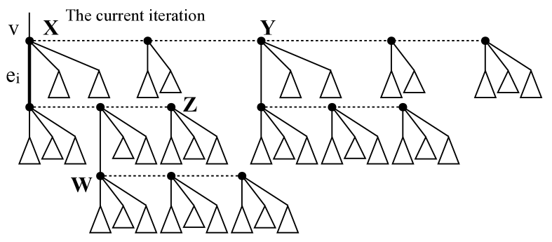
Figure 3:

3.3 Correctness of the algorithm

For any iteration $X$ on $\mathcal{T}$, it is redundant to process safe and conflict edges independently among siblings of the same parent. To avoid this, we simultaneously process these edges by using following concentric structures around the pivot on $X$. Let $k\in\{0,1,2\}$ and $\ell\in\{0,1,2\}$. We define the concentric structure $D_{v}(k,\ell)$ as follows:

$$D_{v}(k,\ell)=\{\{x,y\}\in E(G(X))\mid dist_{G(X)}(x,v)=k,dist_{G(X)}(y,v)=\ell\}.$$ (1)

$D_{v}(k)$ denotes $D_{v}(k,k)\sqcup D_{v}(k,k+1)$. We call an edge $e\in D_{v}(k,\ell)$ a $k$-$\ell$ edge of $v$ and an edge $e\in D_{v}(k)$ a $k$-$*$ edge of $v$. Figure 4 (a) shows an example of $0$-$1$ edges, $1$-$*$ edges, and $2$-$*$ edges. The distance between two vertices is defined by the length of shortest path in not $G$ but $G(X)$. The next lemma implies that $M(X)\cup\{e\}$ is an induced matching in $G$ for any edge $e\in D_{v}(0)$. A proof of the next lemma is shown in Appendix A.

Lemma 2.

Let $G$ be an input graph, $X$ be any iteration in the algorithm EIM in Algorithm 1, and $e$ be any edge in $D_{v}(0)$. Then, $M(X)\cup\{e\}$ is an induced matching in $G$.

Since EIM outputs a solution in a leaf iteration and $M(X)$ is induced matching for each iteration $X\in\mathcal{T}$, the following corollary holds from Lemma 2.

Corollary 3.

The algorithm EIM in Algorithm 1 outputs only induced matchings.

Next, we consider a method for obtaining $G(X.i)$. For any $0$-$1$ edge $e_{i}=\{v,u_{i}\}$ of a pivot $v$, we define $Sect_{e_{i}}(k)$ as follows:

$$Sect_{e_{i}}(k)=\{f\in D_{v}(k)\mid dist_{G(X)}(v,f)=k,dist_{G(X)}(e_{i},f)=k-1\}.$$ (2)

We show an example of $Sect_{e_{i}}(k)$ in Figure 4. Proofs of the following two lemmas are shown in Appendix A.

Lemma 4.

Let $X$ be an iteration in the algorithm EIM in Algorithm 1. Then, $G(X.0)=G(X)\setminus\{v\}$ holds.

Lemma 5.

Let $X$ be any iteration in the algorithm EIM in Algorithm 1 and $i$ be positive integer. Then, $G(X.i)=G(X)\setminus(D_{v}(0)\cup D_{v}(1)\cup Sect_{e_{i}}(2))$ holds.

Lemma 4 and Lemma 5 imply that EIM correctly compute $G(X.i)$ in $X$.

Lemma 6.

The algorithm EIM in Algorithm 1 outputs solutions without duplication.

Proof.

Let $X$ and $Y$ be two distinct leaf iterations. We proceed by contradiction. Suppose that $M(X)=M(Y)$. From the assumption, $X$ and $Y$ are incomparable. Hence, without loss of generality the lowest common ancestor of $X$ and $Y$ always exists. Let $Z$ be the lowest common ancestor of $X$ and $Y$. We consider the following two cases. (1) Suppose that both $X$ and $Y$ are descendants of the type-$0$ child $Z.0$ of $Z$. This contradicts that $Z$ is the lowest common ancestor of $X$ and $Y$. (2) Suppose that at least one of $X$ and $Y$ is a descendant of a type-$1$ child of $Z$. Without loss of generality, $X$ is a descendant of the $i$th child $Z.i$ of $Z$. If $W$ is $Z.j$ or is any descendant of $Z.j$ where $j\neq i$, then $M(W)$ does not include $e_{i}$ and this contradicts $M(X)=M(Y)$. Hence, the statement holds. ∎

Lemma 7.

The algorithm EIM in Algorithm 1 outputs all solutions in $\mathcal{M}$.

Proof.

Let $\mathcal{T}$ be an enumeration tree, $X$ be any iteration on $\mathcal{T}$, and $v$ be the pivot on $X$. From Lemma 4 and Lemma 5, EIM correctly divides a solution set $\mathcal{S}(X)$ in $X$ into $\mathcal{S}_{0}(X),\dots,\mathcal{S}_{d(v)}(X)$. If $\left|\mathcal{S}(X)\right|=1$, then EIM outputs $\mathcal{S}(X)$. Hence, EIM outputs all solutions in $\mathcal{M}$. ∎

From corollary 3, Lemma 6, and, Lemma 7, the next theorem holds.

Theorem 8.

The algorithm EIM in Algorithm 1 enumerates all solutions without duplication.

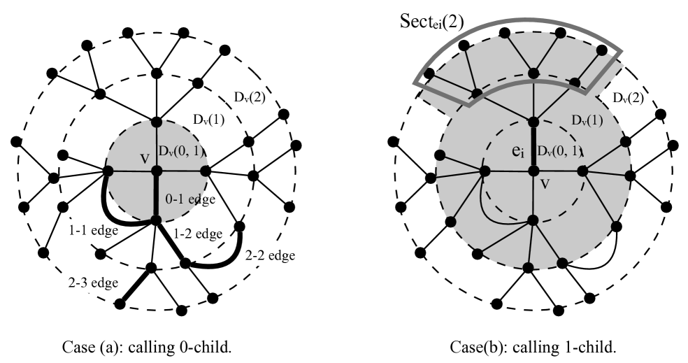
Figure 4: An example of dividing edges by the pivot $v$ in the graph $G$. In case (a), the shaded area indicates the area of edges to be removed when calling type-$0$ child. In case (b), the shaded area indicates the area of edges to be removed when calling type-$1$ child. The area surrounded by the solid line represent $Sect_{e_{i}}(2)$

3.4 Amortized analysis of the time complexity

If the degree of the pivot on $X$ is less than three, then EIM obviously runs in the constant amortized time per solution since the number of steps in each iteration $X$ is constant. Thus, we assume the degree of pivot is at least three.

We first consider the data structure $\mathcal{L}ist(G(X))$ to efficiently extract the set of vertices whose degree is $k$ when we are given $k$. We define $\mathcal{L}ist(G(X))$ as follows: $\mathcal{L}ist(G(X))=\{L_{0},\dots,L_{\Delta(G(X))}\}$, where for any $0\leq i\leq\Delta(G(X))$, $L_{i}=\{v\in V(G)\mid d_{G(X)}(v)=i\}$. The lists in $\mathcal{L}ist(G(X))$ are implemented by doubly-linked lists, and we denote $x\in\mathcal{L}ist(G(X))$ if $\mathcal{L}ist(G(X))$ includes $x$. For any input graph $G$, we can compute $\mathcal{L}ist(G)$ in $O\left(\left|V(G)\right|\right)$ time by using bucket sort. We can implement $\mathcal{L}ist(G(X))$ such that extracting any vertex from $\mathcal{L}ist(G(X))$ can be done in constant time. By using $\mathcal{L}ist(G(X))$, we can see the following lemma. The proof of Lemma 9 in Appendix A.

Lemma 9.

Let $X$ be any iteration in $\mathcal{T}$. Then, we can find the pivot in constant time by using $\mathcal{L}ist(G(X))$.

Next, we define the edge set $D^{\leq}_{v}(2)$ as follows: $D^{\leq}_{v}(2)=D_{v}(0)\cup D_{v}(1)\cup D_{v}(2)$, i.e. $D^{\leq}_{v}(2)$ is the edge set consisting of all edges whose distance is less than two from $v$.

Lemma 10.

Let $G$ be a $C_{4}$-free graph, $v$ be the pivot on an iteration $X$, and, $u$ be a vertex satisfying $dist_{G}(u,v)=2$. Then, the number of edges whose endpoint is $u$ in the set of $1$-$2$ edges of $v$ is exactly one.

Proof.

We proof by contradiction. Let $f_{1}=\{u,w_{1}\}$ and $f_{2}=\{u,w_{2}\}$ be two distinct $1$-$2$ edges whose end point is $u$. We assume $w_{1}\neq w_{2}$. Since $f_{1}$ and $f_{2}$ are $1$-$2$ edges and $dist_{G}(u,v)=2$, $dist_{G}(v,w_{1})=dist_{G}(v,w_{2})=1$ holds. Thus, there exist two edges $e_{1}=\{v,w_{1}\}$ and $e_{2}=\{v,w_{2}\}$. Hence, there is a cycle $(v,e_{1},w_{1},f_{1},u,f_{2},w_{2},e_{2},v)$ in $G$. This contradicts that $G$ is a $C_{4}$-free graph. Hence, the statement holds. ∎

Lemma 11.

Let $G$ be a $C_{4}$-free graph and $v$ be the pivot on an iteration. Then, the following inequality holds: $\sum_{e\in D_{v}(0)}\left|Sect_{e}(2)\right|\leq 2\left|D_{v}(2)\right|$.

Proof.

We show that $\bigcup_{e\in D_{v}(0)}Sect_{e}(2)=D_{v}(2)$. Let $f=\{x,y\}$ be an edge in $Sect_{e}(2)$. By definition, $f\in D_{v}(2)$ holds. Without loss of generality, we can assume that $dist_{G}(x,v)=2$. Since $dist_{G}(x,v)=2$, there is a vertex $w$ satisfying $dist_{G}(x,w)=dist_{G}(w,v)=1$. By definition, $f$ belongs to $Sect_{\{w,v\}}(2)$. Hence, $\bigcup_{e\in D_{v}(0)}Sect_{e}(2)=D_{v}(2)$ holds.

Next, we assume that for any $2$-$*$ edge $f\in D_{v}(2)$, $f$ belongs to the following three sets; $Sect_{e_{1}}(2)$, $Sect_{e_{2}}(2)$, and $Sect_{e_{3}}(2)$ , where $e_{1},e_{2},e_{3}\in D_{v}(0)$. Then, by the definition of $Sect_{e_{i}}(2)$, $dist_{G}(e_{i},f)=1$ holds for $i\in\{1,2,3\}$. Hence, there is some $g_{i}=\{x_{i},y_{i}\}$ satisfying $x_{i}\in e_{i}$ and $y_{i}\in f$. By the definition of $e_{i}$, $dist_{G}(v,x_{i})=1$ and $dist_{G}(v,y_{i})=2$ hold. This implies that $g_{i}$ is a $1$-$2$ edge that shares the end point with $f$. By the pigeonhole principle, one of the end points of $f$ has at least two $1$-$2$ edges. This contradicts with Lemma 10, hence the statement holds. ∎

In the remaining of this section, we show that EIM enumerates all solutions in constant amortized time per solution. To show the complexity, we show that the ratio between the number of $1$-child iterations and $0$-child iterations is constant. If the statement holds, then the number of iterations on $\mathcal{T}$ is linear in the number of leaf iterations of $\mathcal{T}$. Let $X$ be any iteration in $\mathcal{T}$ and $v$ be the pivot on $X$. Suppose that $e=\{x,y\}$ is any edge in $\in D^{\leq}_{v}(2)$ and $f=\{v,x\}$. We denote by $C(X,e)$ a descendant iteration of $X$ such that $Y=C(X,e)$ is the top of the chain including $X$ and receives $M(Y)$ defined as follows.

1. If $e$ is a $0$-$1$ edge, then $M(Y)=M(X)\cup\{e\}$.

2. If $e$ is a $1$-$1$ edge, then $M(Y)=M(X)\cup\{f\}$.

3. If $e$ is a $1$-$2$ edge and $Sect_{f}(2)=\emptyset$, then $M(Y)=M(X)\cup\{e\}$.

4. If $e$ is a $1$-$2$ edge and $Sect_{f}(2)\neq\emptyset$, then $M(Y)=M(X)\cup\{f^{\prime},g\}$, where $f^{\prime}\in D_{v}(0)$ and $g\in Sect_{f}(2)$ such that $f^{\prime}\neq f$ and $dist_{G}(f^{\prime},g)=2$.

5. If $e$ is $2$-$*$ edge, then $M(Y)=M(X)\cup\{e,h\}$, where $h$ is an edge such that $h$ is adjacent to $v$ and $dist_{G}(e,h)=2$.

We call $C(X,e)$ the corresponding iteration to $X$ w.r.t $e$. The next lemma shows that $C(X,e)$ satisfying the above conditions always exists.

Lemma 12.

For any iteration $X$ and $e\in D^{\leq}_{v}(2)$, there always exists the corresponding iteration $C(X,e)$ to $X$ w.r.t $e$.

Proof.

Let $e=(x,y)$. From Lemma 7, to proof the lemma, all we have to do is show that $M(C(X,e))$ is a solution. If (1) or (3.a) holds, then $M(C(X,e))$ is obviously an induced matching since $e\in D^{\leq}_{v}(2)$. Next, we consider condition (2). There are two edges $\{v,x\}=f$ and $\{y,v\}$ since $e$ is a $1$-$1$ edge. Since $f\in D^{\leq}_{v}(2)$, $M(C(X,e))$ is a solution. Next, we consider condition (3.b). Let $f=\{v,x\}$. Since $e$ is a $1$-$2$ edge, such edge $f$ always exists. Let $g$ be any edge in $Sect_{f}(2)$. From Lemma 10, at least one of the end points of $g$ connects exactly one $1$-$2$ edge. Hence, there is an edge $f^{\prime}\neq f$ that is adjacent to $v$ and satisfies $dist_{G}(f^{\prime},g)=2$ since the degree of $v$ is at least three. Moreover, $\{f^{\prime},g\}$ is an induced matching since $dist_{G}(f^{\prime},g)=2$. Hence, $M(C(X,e))$ is an induced matching. Finally, we consider condition (4). Since $d_{G}(v)\geq 3$, there exists an edge $h$ that is adjacent to $v$ and satisfies $dist_{G}(e,h)$. Hence, $M(C(X,e))$ is an induced matching. ∎

In the following lemmas, for any iteration $X$, we show the number of pairs of an iteration and an edge whose corresponding iteration is $X$ is constant.

Lemma 13.

If a graph $G$ is $C_{4}$-free, then the number of $1$-$1$ edges adjacent to $0$-$1$ edges is at most one.

Proof.

We show the lemma by contradiction. Suppose there are two distinct $1$-$1$ edges $f=\{u,w\}$ and $g=\{u,x\}$ that are adjacent to a $0$-$1$ edge $e$. By the definition of a $1$-$1$ edge, $\{u,w,x\}\subseteq N(v)$. Hence, there exist two distinct edges $f^{\prime}=\{v,w\}$ and $g^{\prime}=\{v,x\}$. However, this implies that there exist a $4$-cycle $(v,f^{\prime},w,f,u,g,x,g^{\prime},v)$. This contradicts that $G$ is $C_{4}$-free. Hence, the statement holds. ∎

For the proofs of the next lemmas, see Appendix A.

Lemma 14.

Let $X$ and $e$ be a pair of an iteration on $\mathcal{T}$ and an edge in $D_{v}^{\leq}(2)$ satisfying condition (3.a), and $Y$ be any iteration on $\mathcal{L}$ from $X$ to $C(X,e)$ such that $Y$ satisfies $C(Y,e)=C(X,e)$. Then, the number of such $Y$ is at most two.

Lemma 15.

Let $X$ be any iteration in $\mathcal{T}$. Then, the number of pairs an iteration $Y$ and an edge $e$ satisfying $C(Y,e)=X$ is at most six.

From Lemma 13, Lemma 14, and Lemma 15, for any iteration $X\in\mathcal{T}$, the number of pairs of an iteration $Y$ and an edge $e$ such that $C(Y,e)=X$ is constant. Next, the following lemmas show that total computation time in EIM is $O\left(\left|\mathcal{T}\right|\right)$ time. Let $F(X)$ be $\bigcap_{i=0,\dots,\Delta(G(X))}E(G(X.i))$. That is, $F(X)$ is the set of edges that are shared by all child iterations of $X$.

Lemma 16.

Let $v$ be the pivot on an iteration $X$ in $\mathcal{T}$. Then, $E(G(X))\setminus F(X)=D^{\leq}_{v}(2)$.

Proof.

Let $\{e_{1},\dots,e_{d_{G(X)}(v)}\}$ be the set of edges that are adjacent to $v$. We show $F(X)=E(G(X))\setminus D^{\leq}_{v}(2)$. Firstly, we show $F(X)\subseteq E(G(X))\setminus D^{\leq}_{v}(2)$. For any $i=0,\dots,d_{G(X)}(v)$, $M(G(X.i))$ includes $e_{i}=\{v,u_{i}\}$ by definition. Hence, $F(X)$ does not include conflicting edges of $e_{i}$. In addition, each edge $f\in F(X)$ satisfies $dist_{G(X)}(f,v)\geq 2$ and $dist_{G(X)}(f,u_{i})\geq 2$. Therefore, $f$ is not included in $D^{\leq}_{v}(2)$. Secondly, we show $F(X)\supseteq E(G(X))\setminus D^{\leq}_{v}(2)$. Let $g$ be any edge in $E(G(X))\setminus D^{\leq}_{v}(2)$. By definition, $dist_{G(X)}(g,e_{i})\geq 2$ holds for any $e_{i}$. Therefore, $g\in F(X)$ since $g\in E(G(X.i))$. Now, $D^{\leq}_{v}(2)\subseteq E(G(X))$ and $F(X)\cap D^{\leq}_{v}(2)=\emptyset$. Hence, the statement holds. ∎

Lemma 17.

$\sum_{X\in V(\mathcal{T})}\left|E(G(X))\setminus F(X)\right|$ is bounded by $O\left(\left|\mathcal{T}\right|\right)$.

Proof.

Let $X$ be any iteration and $v$ be the pivot on $X$. The number of iterations $Y=C(X,e)$ is at most $\left|D^{\leq}_{v}(2)\right|$, where $e$ is an edge in $D^{\leq}_{v}(2)$. Hence, the number of all corresponding iterations is equal to $\sum_{X\in V(\mathcal{T})}\left|E(G(X))\setminus F(X)\right|$ since $E(G(X))\setminus F(X)=D^{\leq}_{v}(2)$ from Lemma 16 together with that a pair of an internal iteration $X$ and an edge $e\in D^{\leq}_{v}(2)$ corresponds to exactly one iteration $C(X,e)$. Next, we consider the number of all corresponding iterations. The number of pairs of an iteration $Y$ and an edge $e$ such that $C(Y,e)=X$ is at most constant from Lemma 15. Since the number of internal iteration is $\left|\mathcal{T}\right|$, the number of all corresponding iterations is bounded by $O\left(\left|\mathcal{T}\right|\right)$, Hence, the statement holds. ∎

Theorem 18.

The algorithm EIM in Algorithm 1 enumerates all induced matchings in constant amortized time per solution in a $C_{4}$-free graph $G$ after $O\left(\left|V\right|+\left|E\right|\right)$ preprocessing time.

Proof.

The correctness of EIM is obvious from Lemma 8. Next, we consider the time complexity of EIM. Let $X$ be an iteration of EIM. In the preprocessing phase, EIM constructs $\mathcal{L}ist(G)$ in $O\left(\left|V\right|+\left|E\right|\right)$ time by using bucket sort. Next, we consider the total time for deleting edges in an input graph. Each edge is deleted at most twice from Lemma 10 in each iteration. Moreover, from Lemma 17, the total number of deleted edges is $O\left(\left|\mathcal{T}\right|\right)$ in EIM. Hence, the total time of edge deletion is $O\left(\left|\mathcal{T}\right|\right)$ time since each edge can be removed in constant time from the input graph. Next, we consider the total time of the updating $\mathcal{L}ist(G(X))$. When EIM removes an edge $e=\{u,v\}$ from $X$, EIM moves $u\in L_{i}$ to $L_{i-1}$ and $v\in L_{j}$ to $L_{j-1}$. Since it can be done in constant time, the time complexity of EIM is $O\left(\left|\mathcal{T}\right|\right)$. In addition, every iteration $X$ in $\mathcal{T}$ has a child at least two. Hence, the number of solutions is $\Omega(\left|\mathcal{T}\right|)$. Therefore, EIM runs in $O\left(\left|\mathcal{T}\right|/\left|\mathcal{T}\right|\right)=O\left(1\right)$ time per solution. ∎

4 Counting of Induced Matchings for Other Graph Classes

To complement the result of Sec. 3, in this section, we present some fixed-parameter tractability results on counting the number of induced matchings in terms of descriptive complexity theory [10]. See Appendix B for omitted definitions and proofs. Recently, Frick [11] introduced the notion of locally tree-decomposability by generalizing the tree decomposition. He showed the fact that the classes of graphs of bounded degree, of bounded tree-width, and planar graphs are locally tree-decomposable [11].

Proposition 19 (Frick [11]).

Let $\mathcal{C}$ be any class of locally tree-decomposable structures. For any structure $\mathcal{A}\in\mathcal{C}$, a counting problem $\Pi$ definable in FO can be solved in linear time in $||\mathcal{A}||$, where $\mathcal{A}$ is given with its underlying nice tree cover $\mathcal{T}$ associated with $r,\ell,g$.

For any $k\geq 0$, a $k$-induced matching is an induced matching $M\subseteq E$ with $|M|=k$. From the above fact and Proposition 31, we show the next theorem.

Theorem 20.

For any class $\mathcal{G}$ of graphs of bounded degree, graphs of bounded tree-width, or planar graphs and any $k\geq 0$, the counting problem of $k$-induced matchings in an input graph $G$ in $\mathcal{G}$ can be solved in linear time in $||G||$.

In the proof, we built a FO-formula $\phi$ describing that an edge subset is a $k$-induced matching. Hence, the counting problem of $k$-induced matchings belongs to FPT when parameterized with some constants determined by $k$, $\phi$, and $\mathcal{G}$.

5 Conclusion

In this paper, we presented an efficient algorithm for enumerating all induced matchings in constant amortized time for $C_{4}$-free graphs. Generalization of this result to other graph classes is an interesting future work. Investigating the other class of induced subgraphs such as induced paths is also interesting. We also have interests in the independent set enumeration in the square of line graphs[3] and also counting problems of these structures.

Acknowledgements

This research was supported by Grant-in-Aid for Scientific Research(A) Number 16H01743.

Appendix A Appendix (Proof of some lemmas)

In this appendix, we show proofs of Lemma 1, Lemma 2, Lemma 4, Lemma 5, and Lemma 9.

Lemma 21.

Let $X$ and $Y$ be any iterations. If $X\preceq Y$ then $M(X)\subseteq M(Y)$ and $E(G(X))\supseteq E(G(Y))$ hold. (A proof of Lemma 1. )

Proof.

There is a downward path $\mathcal{L}$ from $X$ to $Y$ since $X\preceq Y$. It is obvious that EIM does not remove any edge in $M(X)$ from $M(X^{\prime})$ in $X^{\prime}\in\mathcal{L}$. On the other hands, EIM does not add any edge to $E(G(X))$ to $E(G(X^{\prime}))$ in $X^{\prime}\in\mathcal{L}$. ∎

Lemma 22.

Let $G$ be an input graph, $X$ be any iteration in the alglrithm EIM in Algorithm 1, and $e$ be any edge in $D_{v}(0)$. Then, $M(X)\cup\{e\}$ is an induced matching in $G$. (A proof of Lemma 2. )

Proof.

We proof by contradiction. Assume that there is a conflicting edge $f\in M(X)$ with $e$. From Lemma 1, there is an iteration $Y\preceq X$ such that $f$ is added to $M(Y)$. Since $f$ conflict with $e$, either (1) $e$ is adjacent to $f$ or (2) $e$ is not adjacent to $f$ and there is an edge $g$ in $G(Y)$ that is adjacent to both $e$ and $f$. We consider case (1). By the definition of $G(Y)$, if EIM adds $f$ to $M(Y)$ in $Y$, edges adjacent to $f$ are not in $G(W)$, for any descendant iteration $W$ of $Y$. This contradicts the assumption. Next, we consider case (2). If $g\in G(Y)$ holds, then $dist_{G(Y)}(e,g)=1$. This implies that for any descendant iteration $W$ of $Y$, $e\notin G(W)$. On the other hands, if $g\notin G(Y)$, then $G(Y)$ is not induced subgraph since $e,f\in G(Y)$ and $g\notin G(Y)$. This also contradicts the assumption. Hence the statement holds. ∎

Lemma 23.

Let $X$ be an iteration in the algorithm EIM in Algorithm 1. Then, $G(X.0)=G(X)\setminus\{v\}$ holds. (A proof of Lemma 4. )

Proof.

Since $M(X)=M(X.0)$, there is no edge in $G(X.0)$ such that one of its endpoint is $v$. Thus, the statement holds. ∎

Lemma 24.

Let $X$ be any iteration in the algorithm EIM in Algorithm 1 and $i$ be positive integer. Then, $G(X.i)=G(X)\setminus(D_{v}(0)\cup D_{v}(1)\cup Sect_{e_{i}}(2))$ holds. (A proof of Lemma 5. )

Proof.

For any edge $f$ in $G$, we show that the following cases are equivalent: (1) $f$ is conflicting edge of $e$ and (2) $f$ belongs to $D_{v}(0)\cup D_{v}(1)\cup Sect_{e_{i}}(2)$. Let $e_{i}=\{v,v_{i}\}$ and $f=\{u,w\}$. Without loss of generality, we can assume that $dist_{G}(u,v)\leq dist_{G}(w,v)$. If $f\notin D_{v}(0)\cup D_{v}(1)\cup Sect_{e_{i}}(2)$, then $1<dist_{G}(u,v)\leq dist_{G}(w,v)$ and $1<dist_{G}(u,v_{1})\leq dist_{G}(w,v_{1})$ hold. Hence, $f$ does not conflict with $e_{i}$. On the other hands, if $f\notin D_{v}(0)\cup D_{v}(1)\cup Sect_{e_{i}}(2)$ then $f$ obviously conflicts with $e_{i}$. Hence, the statement holds. ∎

Lemma 25.

Let $X$ be any iteration in $\mathcal{T}$. Then, we can find the pivot in constant time by using $\mathcal{L}ist(G(X))$. (A proof of Lemma 9. )

Proof.

It is obvious that $\bigsqcup_{L_{i}\in\mathcal{L}ist(G(X))}=V(G)$ holds. $i_{*}=\mathop{\rm arg~{}max}\limits_{i\in\{0,\dots,\Delta(G(X))\}}(L_{i}\neq\emptyset)$, that is, $L_{i_{*}}$ is the non empty list with the maximum index in $\mathcal{L}ist(G(X))$. Now, the pivot on $X$ is in $L_{i_{*}}$ since $\Delta(G(X))=i_{*}$. Hence, EIM can obtain $v$ in constant time by extracting a vertex from the tail of $L_{i_{*}}$. ∎

Lemma 26.

Let $X$ and $e$ be a pair of an iteration on $\mathcal{T}$ and an edge in $D_{v}^{\leq}(2)$ satisfying condition (3.a), and $Y$ be any iteration on $\mathcal{L}$ from $X$ to $C(X,e)$ such that $Y$ satisfies $C(Y,e)=C(X,e)$. Then, the number of such $Y$ is at most two. (A proof of Lemma 14. )

Proof.

We first show that $\mathcal{L}$ consists of $0$-branches except the end of $\mathcal{L}$. By the definition of $C(X,e)$, the end of $\mathcal{L}$ is a $1$-branch since $C(X,e)$ is the top of a chain. Next, $\mathcal{L}$ includes exactly one $1$-branch since $M(C(X,e))=M(X)\cup\{e\}$. Hence, $\mathcal{L}$ consists of only $0$-branch other than the end of $\mathcal{L}$.

By using the above observation, we proof by contradiction. Suppose that there exists three distinct iterations $Y_{1}$, $Y_{2}$, and $Y_{3}$ such that they satisfy condition (3.a) and $C(X,e)=C(Y_{1},e)=C(Y_{2},e)=C(Y_{3},e)$. Thus, for any $i=1,2,3$, $e$ is a $1$-$2$ edge of $v_{i}$ that is the pivot of $Y_{i}$. Let $e=\{x,y\}$ and $f_{i}$ be an edge such that $f_{i}$ shares the end point with $e$ and $f_{i}$ is adjacent to $v_{i}$. Without loss of generality, we can assume $f_{1}=\{x,v_{1}\}$ and $Y_{1}\preceq Y_{2}$, $Y_{1}\preceq Y_{3}$. For $j=2,3$, if $G(Y_{j})$ has the edge $f_{j}=\{y,v_{j}\}$, then this contradict with $Sect_{f_{i}}(2)=\emptyset$. Hence, $v_{j}$ is a neighbor of $x$. In $Y_{1}$, the number of $1$-$1$ edges adjacent to $f_{1}$ is at most one from Lemma 13. Hence, at least one of $f_{2}$ and $f_{3}$ is a $1$-$2$ edge. Without loss of generality, we can assume that $f_{2}$ is a $1$-$2$ edge. Since $Sect_{f_{1}}(2)=\emptyset$, $D_{G(Y_{1})}(v_{3})=1$. In addition, in $Y_{3}$, $d_{G(Y_{3})}(x)\geq 2$ since $x$ is adjacent to $y$ and $v_{3}$. However, this contradicts with $d_{G(Y_{3})}(v_{3})\geq d_{G(Y_{3})}(x)$. Hence, the statement holds. ∎

Lemma 27.

Let $X$ be any iteration in $\mathcal{T}$. Then, the number of pairs an iteration $Y$ and an edge $e$ satisfying $C(Y,e)=X$ is at most six. (A proof of Lemma 15. )

Proof.

Let $\mathcal{L}$ be the path from the root iteration $I$ on $\mathcal{T}$ to $X$ and $X^{\prime}$ be the parent iteration of $X$. Without loss of generality, we can assume that $X$ is the top of a chain by the definition of $C(Y,e)$. Let $X^{\prime\prime}$ be the parent of the top of a chain including $X^{\prime}$ and $\mathcal{L}^{\prime}$ be the path from $X^{\prime\prime}$ to $X^{\prime}$. By the definition of $C(Y,e)$, $Y$ satisfying $C(Y,e)=X$ exists only on $\mathcal{L}^{\prime}$. If $Y$ is $X^{\prime}$, then the number of edges $e^{\prime}$ satisfying $C(Y,e^{\prime})=X$ is at most two by conditions (1) and (2). If $Y$ is $X^{\prime\prime}$, then the number of edges $e^{\prime}$ satisfying $C(Y,e^{\prime})=X$ is at most two by conditions(3.b) and (4). If $Y$ is not $X^{\prime}$ and $X^{\prime\prime}$, then the number of $Y$ satisfying $C(Y,e)=X$ is at most two from Lemma 14. Hence, the statement holds. ∎

Appendix B Appendix (The descriptive parameterized complexity of counting problems)

In this section, we will give the proof of Theorem 20 in Sec. 4. See literatures [10] There are some generic fixed-parameter tractability results for counting problems formulated in terms of descriptive complexity theory [10]. In 1991, Arnborg and Seese showed that the counting problems definable in monadic second-order logic (MSO) can be solved in linear time when the input structures have bounded tree-width [10]. By extending these results, Frick [11] showed that the counting problems definable in first-order logic (FO) can be solved in linear time on locally tree-decomposable classes of structures.

Formally, their result is summarized as follows. A parameterized counting problem is formulated as a problem of, given an instance $I$ and a parameterization $k\geq 0$, a parameterization of $I$, returning a number $F(I)\geq 0$. We say that a counting problem parameterized with $k$ belongs to FPT if there exist some computable function $f$ and constant $c>0$ such that the problem can be solved in $O(f(k)\,n^{c})$ time, where $n$ is the input size [10].

We introduce the language of first-order logic (FO) as follows [10]. Let $\tau$ be the vocabulary of graphs. For a graph $G=(V,E)$, we assume that the corresponding FO-structure $\mathcal{A}=(A,\dots)$ includes the domain $A:=V\cup E$ for vertices and edges, and the incident relation $\textit{IND}\subseteq E\times V\times V$ defined later. We also assume that the vocabulary $\tau$ for graphs includes the ternary relation IND such that $\textit{IND}(e,x,y)$ $\iff$ an edge $e$ has end points $x$ and $y$. The set $FO[\tau]$ of first-order formulas is built up from countably many sorted first-order variables $x,y,x_{1},\dots$ for vertices and $e,f,e_{1},\dots$ for edges, the predicate symbols IND for incidencet relation, $=$ for equality, and $P_{1},P_{2},\dots\in\tau$, connectives $\lor,\land,\neg,\to$, and quantifiers $\exists x,\forall x$ ranging over indivisuals. We assume the standard semantics of FO-formulas [11].

A decision problem $\Pi$ is definable in FO on vocabulary $\tau$for a class $\mathcal{C}$ of structures if and only if there exists a FO-formula $\phi(\bar{x})\in FO[\tau]$ with some $m$-vector of free variables $\bar{x}=(x_{1},\dots,x_{m})$ such that for all structure $\mathcal{A}\in\mathcal{C}$, the answer of $\Pi$ is yes on $\mathcal{A}$ $\iff$ there exists some $m$-tuple $\bar{a}=(a_{1},\dots,a_{m})\in A^{m}$ such that $\mathcal{A}\models\phi(\bar{a})$ holds. Similarly, we introduce the FO-definability of counting problems as follows.

Definition 28 ([11, 10]).

A counting problem $\Pi$ is definable in FO if there exists a FO-formula $\phi(\bar{x})\in FO[\tau]$ with some $\bar{x}=(x_{1},\dots,x_{m})$ such that the answer (the number of solutions in $\Pi$) is given by the number of $\bar{a}\in A^{m}$ such that $\mathcal{A}\models\phi(\bar{a})$.

Extending the notion of tree-decomposition [10], Frick [11] gave a sufficient condition, called locally tree-decomposability, so that a counting problems definable in the first-order logic (FO) belongs to FPT. Let $\tau$ be a vocabulary and $\mathcal{A}$ a $\tau$-structure with domain $A$. The Gaifman graph of $\mathcal{A}$ is the graph $\mathcal{G}(\mathcal{A})=(A,F)$, where the vertex set is $A$, and for every $a,b\in A$, $(a,b)\in F$ $\iff$ $a$ and $b$ appear in the same tuple of some relation in $\mathcal{A}$. We denote by $d^{\mathcal{A}}(a,b)$ the distance between $a$ and $b$ in $\mathcal{G}(\mathcal{A})$. For any $r\geq 1$ and element $a\in A$, we define the $r$-neighborhood of $a$ by the set $N^{\mathcal{A}}_{r}(a):=\{b\in A\mid d^{\mathcal{A}}(a,b)\leq r\}$. For any set $X\subseteq A$, we define $N^{\mathcal{A}}_{r}(X):=\bigcup_{a\in X}N^{\mathcal{A}}_{r}(a)$. Let $\mathcal{A}$ be a structure with domain $A$. Let $r,\ell\geq 1$ be any integers and $g:N\to N$ be any function. A nice $(r,\ell,g)$-tree cover of a structure $\mathcal{A}$ is a class $\mathcal{T}$ of subsets of $A$ such that:

1. For any $a\in A$, there exists some $U\in\mathcal{T}$ such that $N^{\mathcal{A}}_{r}(a)\subseteq U$.

2. For any $U\in\mathcal{T}$, there are less than $\ell$ sets $V\in\mathcal{T}$ such that $U\cap V\not=\emptyset$.

3. For all $U_{1},\dots,U_{q}\in\mathcal{T}$ and $q\geq 1$, the tree-width of the induced structure $\langle U_{1}\cup\dots\cup U_{q}\rangle^{\mathcal{A}}$ is $g(q)$ or less.

Definition 29 (Frick [11]).

A class $\mathcal{C}$ of structures is locally tree-decomposable if there is a linear time algorithm that, given structure $\mathcal{A}\in\mathcal{C}$ and $r\geq 1$, computes a nice $(r,\ell,g)$-cover of $\mathcal{A}$ for suitable $\ell=\ell(r)$ and $g=g_{r}$ depending only on $r$.

In the above definition, the parameter $r$ corresponds to the radius of predicates in Gaifman’s Theorem on the locality of FO-formulas [10].

Lemma 30 (Frick [11]).

The classes of graphs of bounded degree, of bounded tree-width, and planar graphs are locally tree-decomposable.

In the followings, we denote by $||G||=m+n$ the size of an input graph $G$.

Proposition 31 (Frick [11]).

Let $\mathcal{C}$ be any class of locally tree-decomposable structures. For any structure $\mathcal{A}\in\mathcal{C}$, a counting problem $\Pi$ definable in FO can be solved in linear time in $||\mathcal{A}||$, where $\mathcal{A}$ is given with its underlying nice $(r,\ell,g)$-tree cover $\mathcal{T}$ associated with $r,\ell,g$.

From the proof of Proposition 31 in [11], we can see that the running time of the algorithm to solve the the counting problem is $O(f(k)n^{c})$ for some function $f$ and constant $c$, where the parameter $k$ is determined by on $r,\ell,g$, the nice $(r,\ell,g)$-tree cover $\mathcal{T}$, and the size $||\phi||$ of the formula $\phi$. Note that $f$ is even not elementary in general [11].

For any $k\geq 0$, a $k$-induced matching in a graph $G=(V,E)$ is an induced matching $M\subseteq E$ with $|M|=k$. Now, we show the main results of this section.

Theorem 32.

For any class $\mathcal{G}$ of graphs of bounded degree, graphs of bounded tree-width, or planar graphs and any $k\geq 0$, the counting problem of $k$-induced matchings in an input graph $G$ in $\mathcal{G}$ can be solved in linear time in $||G||$. (A proof of Theorem 20. )

Proof.

To prove the theorem, it is sufficient to give a FO-formula $\phi(e_{1},\dots,e_{k})$ such that $G\models\phi(e_{1},\dots,e_{k})$ $\iff$ the set $M=\{e_{1},\dots,e_{k}\}$ is an induced matching in $G$. We give auxiliary predicates as follows. First, the predicate

$$\textit{DISJ}(e_{1},\dots,e_{k}) \equiv \bigwedge_{1\leq i<j\leq k}\neg(e_{i}=e_{j})$$

states that edges $e_{1},\dots,e_{k}$ are mutually distinct. Secondly, the predicate

$$\textit{CONN}(e,f,g) \equiv \exists x_{1},\exists x_{2},\exists y_{1},\exists y_{2},\exists z_{1},\exists z_{2}\;$$

$$\left\{\begin{array}[]{l}\textit{IND}(e,x_{1},x_{2})\land\textit{IND}(f,y_{1},y_{2})\land\\ \left[\begin{array}[]{l}(\textit{IND}(g,z_{1},z_{2})\land\;\bigvee_{i,j\in\{1,2\}}(x_{i}=z_{1})\land(y_{j}=z_{2})\;)\\ \lor(x_{1}=y_{1})\lor(x_{2}=y_{2})\end{array}\right]\end{array}\right\}.$$

states that given edges $e$ and $f$ are connected by another given edge $g$. Using CONN, we then define the predicate

$$\textit{SAFE}(e_{1},\dots,e_{k}) \equiv \bigwedge_{1\leq i<j\leq k}\neg\left\{\begin{array}[]{c}\exists g\,\textit{CONN}(e_{i},e_{j},g)\end{array}\right\}$$

which states that there is no edge connecting any pair of distinct edges in $\{e_{1},\dots,e_{k}\}$. Combining these predicates, we build the desired predicate

$$\phi(e_{1},\dots,e_{k}) \equiv \textit{DISJ}(e_{1},\dots,e_{k})\land\textit{SAFE}(e_{1},\dots,e_{k})$$

Hence, it follows from Lemma 30 and Proposition 31 that for any $G=(V,E)$, we can compute the number $N_{k}$ of $k$-tuples $\bar{e}=(e_{1},\dots,e_{k})\in E^{k}$ with $G\models\phi(\bar{e})$ in linear time in $||G||=m+n$. Since there are exactly $k!$ permutations of $\{e_{1},\dots,e_{k}\}$, we can obtain the number of $k$-induced matchings in $G$ as $N_{k}$ devided by $k!$. ∎

From the proof of the above theorem, we see that the counting problem of $k$-induced matchings belongs to FPT when parameterized with $k$ and some constants determined by the nice local tree decomposition for an input class $\mathcal{G}$. It is not hard to see that the formula $\phi$ in the proof can be written in the form $\phi(\bar{e})\equiv\forall\bar{x}\,\psi(\bar{e},\bar{x})$ for a quantifier-free FO-formula $\psi$. Thus, it is in FO-$\Pi_{1}$.

References

- [1] S. Arnborg, J. Lagergren, and D. Seese. Easy problems for tree-decomposable graphs. Journal of Algorithms, 12(2):308–340, 1991.
- [2] A. Brandstädt and C. T. Hoàng. Maximum induced matchings for chordal graphs in linear time. Algorithmica, 52(4):440–447, 2008.
- [3] K. Cameron. Induced matchings. Discrete Appl. Math., 24(1-3):97–102, 1989.
- [4] R. Curticapean and D. Marx. Complexity of counting subgraphs: Only the boundedness of the vertex-cover number counts. In Proc. FOCS 2014, pages 130–139. IEEE, 2014.
- [5] R. Diestel. Graph Theory. Grad. Texts in Math. Springer-Verlag, 4th edition, 2010.
- [6] R. G. Downey and M. R. Fellows. Parameterized complexity. Springer Science & Business Media, 2012.
- [7] J. Edmonds. Paths, trees, and flowers. Canad. J. Math., 17:449–467, 1965.
- [8] M. R. Fellows and M. A. Langston. On search decision and the efficiency of polynomial-time algorithms. In Proc. STOC 1989, pages 501–512. ACM, 1989.
- [9] R. A. Ferreira, R. Grossi, and R. Rizzi. Output-sensitive listing of bounded-size trees in undirected graphs. In Proc. ESA 2011, volume 6942 of LNCS, pages 275–286. Springer, 2011.
- [10] J. Flum and M. Grohe. Parameterized Complexity Theory. Springer, 2006. pages 493.
- [11] M. Frick. Generalized model-checking over locally tree-decomposable classes. Theory of Computing Systems, 37(1):157–191, 2004.
- [12] M. R. Garey and D. S. Johnson. Computers and Intractability; A Guide to the Theory of NP-Completeness. W. H. Freeman & Co., New York, NY, USA, 1990.
- [13] M. C. Golumbic and M. Lewenstein. New results on induced matchings. Discrete Appl. Math., 101(1):157–165, 2000.
- [14] J. E. Hopcroft and R. M. Karp. An algorithm for maximum matchings in bipartite graphs. SIAM J. Comput., 2(4):225–231, 1973.
- [15] V. V. Lozin. On maximum induced matchings in bipartite graphs. Inf.Process.Lett., 81(1):7–11, 2002.
- [16] H. Moser and S. Sikdar. The parameterized complexity of the induced matching problem. Discrete Applied Mathematics, 157(4):715–727, 2009.
- [17] V. Raman and S. Saurabh. Short cycles make w-hard problems hard: Fpt algorithms for w-hard problems in graphs with no short cycles. Algorithmica, 52(2):203–225, 2008.
- [18] R. C. Read and R. E. Tarjan. Bounds on backtrack algorithms for listing cycles, paths, and spanning trees. Networks, 3(5):237–252, 1975.
- [19] L. J. Stockmeyer and V. V. Vazirani. NP-completeness of some generalizations of the maximum matching problem. Inf. Process. Lett., 15(1):14–19, 1982.
- [20] R. E. Tarjan and R. C. Read. Bounds on backtrack algorithms for listing cycles, paths and spanning trees. Networks, 5:237–252, 1975.
- [21] T. Uno. Constant time enumeration by amortization. In Proc. WADS 2015, volume 9214 of LNCS, pages 593–605. Springer, 2015.
- [22] T. Uno. Amortized analysis on enumeration algorithms. In Encyclopedia of Algorithms, pages 72–76. 2016.
- [23] L. G. Valiant. The complexity of computing the permanent. Theor. Comput. Sci., 8(2):189–201, 1979.
- [24] L. G. Valiant. The complexity of enumeration and reliability problems. SIAM Journal on Computing, 8(3):410–421, 1979.