A collocation method for numerical solution of Telegraph equation

Abstract

In this paper, B-spline collocation method is developed for the solution of one-dimensional hyperbolic telegraph equation. The convergence of the method is proved. Also the method is applied on some test examples, and the numerical results have been compared with the analytical solutions. The $L_{\infty}$,$L_{2}$ and Root-Mean-Square errors (RMS) in the solutions show the efficiency of the method computationally.

Department of Mathematics, University of Mohaghegh Ardabili, 56199-11367 Ardabil, Iran.

Keywords: B-spline; Telegraph equation; Collocation method; Convergence.

1 Introduction

Hyperbolic partial differential equations are commonly used in signal analysis for transmission and propagation of electrical signals [1] and also has applications in other fields [2, 3]. In the present paper, a collocation approach based on quintic B-spline functions is utilized for the numerical solution of the one-dimensional hyperbolic telegraph equation. In recent years, many different methods have been used to estimate the solution of the one-dimensional hyperbolic telegraph equation; see, for example, [4-9]. Consider the second-order linear hyperbolic partial differential equation in one-space dimension:

$$\frac{\partial^{2}u}{\partial t^{2}}+2\alpha{\frac{\partial u}{\partial t}}+{\beta^{2}}u={\frac{\partial^{2}u}{\partial x^{2}}}+f(x,t)\ ,\ {a\leq x\leq b}\ ,\ {t\geq 0},$$ (1.1)

with the initial conditions

$$u(x,0)=f_{0}(x),$$ (1.2)

$${\frac{\partial u}{\partial t}}(x,0)=f_{1}(x),$$ (1.3)

and boundary conditions

$$u(a,t)=g_{0}(t),u(b,t)=g_{1}(t),$$ (1.4)

$$\frac{\partial u}{\partial x}(a,t)=g_{2}(t),\frac{\partial u}{\partial x}(b,t)=g_{3}(t),$$ (1.5)

where $\ \alpha$ and $\ \beta$ are constants.
The balance of this paper is organized as follows. In Section 2, the quintic B-spline collocation method for the numerical solution of the one-dimensional hyperbolic telegraph equation is described. In Section 3 we derive convergence of the B-spline collocation method. In Section 4, the results of numerical experiments are presented. A summary is given at the end of the paper in Section 5.

2 Quintic B-spline collocation method

The interval $[a,b]$ is partitioned into a mesh of uniform length $h:=\frac{b-a}{N}$ by the knots $x_{i},i=0,1,\ldots,N$ such that $x_{i}:=x_{0}+ih$ and $a=x_{0}<x_{1}<x_{2}<\ldots<x_{N-1}<x_{N}=b$. To solve the equation (1.1) by collocation method with quintic B-splines as basis functions, we define the approximation $U^{n}(x)$ as following

$$U^{n}(x)=\sum_{i=-2}^{N+2}{c^{n}_{i}B_{i}(x)}.$$ (2.1)

where $U^{n}(x)$ is a shape function that approximates $u(x,t_{n})$ for the time level $t_{n}=nk$ where $k$ is a time step size. For each time level $t_{n}$, the set $\{c^{n}_{-2},c^{n}_{-1},\ldots$ $,c^{n}_{N+1},c^{n}_{N+2}\}$ are unknown real coefficients, which are to be found, and the $B_{i}(x)$ are the quintic B-spline functions defined by [10, 11]

$$B_{i}(x)=\frac{1}{h^{5}}\left\{\begin{array}[]{ll}(x-x_{i-3})^{5},&x\in[x_{i-3},x_{i-2}),\\ (x-x_{i-3})^{5}-6(x-x_{i-2})^{5},&x\in[x_{i-2},x_{i-1}),\\ (x-x_{i-3})^{5}-6(x-x_{i-2})^{5}+15(x-x_{i-1})^{5},&x\in[x_{i-1},x_{i}),\\ (x_{i+3}-x)^{5}-6(x_{i+2}-x)^{5}+15(x_{i+1}-x)^{5},&x\in[x_{i},x_{i+1}),\\ (x_{i+3}-x)^{5}-6(x_{i+2}-x)^{5},&x\in[x_{i+1},x_{i+2}),\\ (x_{i+3}-x)^{5},&x\in[x_{i+2},x_{i+3}),\\ \end{array}\right.$$ (2.2)

where $B_{-2},B_{-1},B_{0},B_{1},\ldots,B_{N+1},B_{N+2}$ form a basis over the region $a\leq x\leq b$. The values of $B_{i}(x)$ and its derivatives may be tabulated as in Table 1. Using approximate function (2.1) and Table 1, we have

$$u(x_{i},t_{n})\approx U^{n}_{i}=c^{n}_{i-2}+26c^{n}_{i-1}+66c^{n}_{i}+26c^{n}_{i+1}+c^{n}_{i+2},$$ (2.3)

$$\frac{\partial u}{\partial x}(x_{i},t_{n})\approx\big{(}U^{\prime}\big{)}^{n}_{i}=\frac{1}{h}(-5c^{n}_{i-2}-50c^{n}_{i-1}+50c^{n}_{i+1}+5c^{n}_{i+2}),$$ (2.4)

$$\frac{\partial^{2}u}{\partial x^{2}}(x_{i},t_{n})\approx\big{(}U^{\prime\prime}\big{)}^{n}_{i}=\frac{1}{h^{2}}(20c^{n}_{i-2}+40c^{n}_{i-1}-120c^{n}_{i}+40c^{n}_{i+1}+20c^{n}_{i+2}).$$ (2.5)

Table 1: $B_{i}$,$B^{{}^{\prime}}_{i}$ and $B^{{}^{\prime\prime}}_{i}$ at the node points.

$x$	$x_{i-3}$	$x_{i-2}$	$x_{i-1}$	$x_{i}$	$x_{i+1}$	$x_{i+2}$	$x_{i+3}$
$B_{i}(x)$	0	1	26	66	26	1	0
$hB^{\prime}_{i}(x)$	0	5	50	0	-50	-5	0
$h^{2}B^{\prime\prime}_{i}(x)$	0	20	40	-120	40	20	0

To apply the proposed method, discretizing the time derivative in the usual finite difference way, with using following finite difference formulae [12], we can write:

$$\big{(}\frac{\partial^{2}u}{\partial t^{2}}\big{)}^{n}_{i}\approx\frac{u^{n+1}_{i}-2u^{n}_{i}+u^{n-1}_{i}}{\Gamma(k)^{2}},$$ (2.6)

$$\big{(}\frac{\partial u}{\partial t}\big{)}^{n}_{i}\approx\frac{u^{n+1}_{i}-u^{n-1}_{i}}{2\Gamma(k)},$$ (2.7)

$$\big{(}\frac{\partial^{2}u}{\partial x^{2}}\big{)}^{n}_{i}\approx\frac{\big{(}\frac{\partial^{2}u}{\partial x^{2}}\big{)}^{n-1}_{i}+\big{(}\frac{\partial^{2}u}{\partial x^{2}}\big{)}^{n+1}_{i}}{2},$$ (2.8)

where $k$ is a time step size, $\big{(}\frac{\partial^{2}u}{\partial x^{2}}\big{)}^{n}_{i}:=\frac{\partial^{2}u}{\partial x^{2}}(x_{i},t_{n})$, $u^{n}_{i}:=u(x_{i},t_{n})$ and $\Gamma(k)$ is a selected function of $k$ satisfying the following equation

$$\Gamma(k)^{2}=(k)^{2}(1+\mathcal{O}(k)^{j}),\hskip 12.80365ptj=0,1,\ldots.$$ (2.9)

In the numerical computations, we applied the following two possible choices for $\Gamma(k)$ to improve the accuracy: $k$ and $2\sin(\frac{k}{2})$. Hence (1.1) can be written as:

$$\frac{u^{n+1}_{i}-2u^{n}_{i}+u^{n-1}_{i}}{\Gamma(k)^{2}}+2\alpha\frac{u^{n+1}_{i}-u^{n-1}_{i}}{2\Gamma(k)}+\beta^{2}u^{n}_{i}=\frac{\big{(}\frac{\partial^{2}u}{\partial x^{2}}\big{)}^{n-1}_{i}+\big{(}\frac{\partial^{2}u}{\partial x^{2}}\big{)}^{n+1}_{i}}{2}+f(x_{i},t_{n}).$$ (2.10)

Rearranging the terms and simplifying we get

$$vu_{i}^{n+1}+w\big{(}\frac{\partial^{2}u}{\partial x^{2}}\big{)}_{i}^{n+1}=\Phi^{n}(x_{i}),$$ (2.11)

where

$$\Phi^{n}(x_{i}):=\Big{(}2-\big{(}\beta\Gamma(k)\big{)}^{2}\Big{)}u^{n}_{i}+\big{(}\alpha\Gamma(k)-1\big{)}u^{n-1}_{i}+\frac{\Gamma(k)^{2}}{2}\big{(}\frac{\partial^{2}u}{\partial x^{2}}\big{)}^{n-1}_{i}+\Gamma(k)^{2}f(x_{i},t_{n}),$$ (2.12)

$$v:=1+\alpha\Gamma(k),$$ (2.13)

$$w:=-\frac{\Gamma(k)^{2}}{2}.$$ (2.14)

Substituting the approximate solution $U$ for $u$ and putting the values (2.3) and (2.5) in (2.11) yields the following difference equation with the variables $c_{i},i=-2,\ldots,N+2$.

$$vU_{i}^{n+1}+w\big{(}U^{\prime\prime}\big{)}_{i}^{n+1}=$$

$$(v+20\frac{w}{h^{2}})c^{n+1}_{i+2}+(26v+40\frac{w}{h^{2}})c^{n+1}_{i+1}+(66v-120\frac{w}{h^{2}})c^{n+1}_{i}$$

$$+(26v+40\frac{w}{h^{2}})c^{n+1}_{i-1}+(v+20\frac{w}{h^{2}})c^{n+1}_{i-2}=\Psi^{n}_{i},\,\,i=0,\ldots,N,$$ (2.15)

where

$$\Psi^{n}_{i}:=\Big{(}2-\big{(}\beta\Gamma(k)\big{)}^{2}\Big{)}U^{n}_{i}+\big{(}\alpha\Gamma(k)-1\big{)}U^{n-1}_{i}$$

$$+\frac{\Gamma(k)^{2}}{2}\big{(}U^{\prime\prime}\big{)}^{n-1}_{i}+\Gamma(k)^{2}f(x_{i},t_{n}).$$ (2.16)

The system (2) consists of $(N+1)$ linear equations in $(N+5)$ unknowns $\widetilde{C}:=\{c_{-2},c_{-1},...,c_{N+1},c_{N+2}\}$. To obtain a unique solution for $\widetilde{C}$ we must use the boundary conditions. From the boundary conditions we can write

$$c^{n+1}_{-2}+26c^{n+1}_{-1}+66c^{n+1}_{0}+26c^{n+1}_{1}+c^{n+1}_{2}=g_{0}(t_{n+1}),$$ (2.17)

$$c^{n+1}_{N-2}+26c^{n+1}_{N-1}+66c^{n+1}_{N}+26c^{n+1}_{N+1}+c^{n+1}_{N+2}=g_{1}(t_{n+1}),$$ (2.18)

and

$$\frac{1}{h}(-5c^{n+1}_{-2}-50c^{n+1}_{-1}+50c^{n+1}_{1}+5c^{n+1}_{2})=g_{2}(t_{n+1}),$$ (2.19)

$$\frac{1}{h}(-5c^{n+1}_{N-2}-50c^{n+1}_{N-1}+50c^{n+1}_{N+1}+5c^{n+1}_{N+2})=g_{3}(t_{n+1}).$$ (2.20)

By using (2.17)-(2.20), we obtain

$$c^{n+1}_{-1}=-\frac{33}{8}c^{n+1}_{0}-\frac{9}{4}c^{n+1}_{1}-\frac{1}{8}c^{n+1}_{2}+\frac{hg_{2}(t_{n+1})}{80}+\frac{g_{0}(t_{n+1})}{16},$$ (2.21)

$$c^{n+1}_{-2}=\frac{165}{4}c^{n+1}_{0}+\frac{65}{2}c^{n+1}_{1}+\frac{9}{4}c^{n+1}_{2}-\frac{13hg_{2}(t_{n+1})}{40}-\frac{5g_{0}(t_{n+1})}{8},$$ (2.22)

$$c^{n+1}_{N+1}=-\frac{33}{8}c^{n+1}_{N}-\frac{9}{4}c^{n+1}_{N-1}-\frac{1}{8}c^{n+1}_{N-2}-\frac{hg_{3}(t_{n+1})}{80}+\frac{g_{1}(t_{n+1})}{16},$$ (2.23)

$$c^{n+1}_{N+2}=\frac{165}{4}c^{n+1}_{N}+\frac{65}{2}c^{n+1}_{N-1}+\frac{9}{4}c^{n+1}_{N-2}+\frac{13hg_{3}(t_{n+1})}{40}-\frac{5g_{1}(t_{n+1})}{8}.$$ (2.24)

Hence we have the following system consists of $(N+1)$ linear equations in $(N+1)$ unknowns $\{c_{0},c_{1},...,c_{N-1},c_{N}\}$. The B-spline method in matrix form can be written as follows :

$$AC=Q,$$ (2.25)

where

$$\mathbf{A}:=$$

$$\left(\begin{array}[]{cccccccccccc}\acute{c}-\frac{33\acute{b}}{8}+\frac{165\acute{a}}{4}&\frac{65\acute{a}}{2}-\frac{5\acute{b}}{4}&\frac{13\acute{a}}{4}-\frac{\acute{b}}{8}&0&\ldots&0\\ \acute{b}-\frac{33\acute{a}}{8}&\acute{c}-\frac{9\acute{a}}{4}&\acute{b}-\frac{\acute{a}}{8}&a&0&\ldots&0\\ \acute{a}&\acute{b}&\acute{c}&\acute{b}&\acute{a}&\ldots&0\\ \vdots&\ddots&\ddots&\ddots&\ddots&\ddots&\vdots&\\ 0&\ldots&\acute{a}&\acute{b}&\acute{c}&\acute{b}&\acute{a}\\ 0&\ldots&0&\acute{a}&\acute{b}-\frac{33\acute{a}}{8}&\acute{c}-\frac{9\acute{a}}{4}&\acute{b}-\frac{\acute{a}}{8}\\ 0&\ldots&0&0&\acute{c}-\frac{33\acute{b}}{8}+\frac{165\acute{a}}{4}&\frac{65\acute{a}}{2}-\frac{5\acute{b}}{4}&\frac{13\acute{a}}{4}-\frac{\acute{b}}{8}\\ \end{array}\right),$$ (2.33)

$$C:=\Big{(}c^{n+1}_{0},c^{n+1}_{1},\ldots,c^{n+1}_{N-1},c^{n+1}_{N}\Big{)}^{T},$$ (2.34)

and

$$\mathbf{Q}:=\left(\begin{array}[]{cccccccccccc}\Psi^{n}(x_{0})+(-\frac{bh}{80}+\frac{13ah}{40})g_{2}(t_{n+1})+(-\frac{b}{16}+\frac{5a}{8})g_{0}(t_{n+1})\\ \Psi^{n}(x_{1})-\frac{ha}{80}g_{2}(t_{n+1})-\frac{a}{16}g_{0}(t_{n+1})\\ \Psi^{n}(x_{2})\\ \vdots\\ \Psi^{n}(x_{N-2})\\ \Psi^{n}(x_{N-1})+\frac{ha}{80}g_{3}(t_{n+1})-\frac{a}{16}g_{1}(t_{n+1})\\ \Psi^{n}(x_{N})+(\frac{bh}{80}-\frac{13ah}{40})g_{3}(t_{n+1})+(-\frac{b}{16}+\frac{5a}{8})g_{1}(t_{n+1}))\\ \end{array}\right),$$ (2.35)

with

$$\acute{a}:=v+20\frac{w}{h^{2}},$$ (2.36)

$$\acute{b}:=26v+40\frac{w}{h^{2}},$$ (2.37)

$$\acute{c}:=66v-120\frac{w}{h^{2}}.$$ (2.38)

The computer algebra system $Mathematica$-$9$ is used for solving the system (2.25). To start any computation, it is necessary to know the value of $u$ at the nodal points of first time level, that is, at $t=k$. A Taylor series expansion at $t=k$ may be written as

$$u(x,k)=f_{0}(x)+kf_{1}(x)+\frac{k^{2}}{2}\big{(}f(x,0)-\beta^{2}f_{0}(x)-2\alpha f_{1}(x)+\frac{\partial f_{0}(x)}{\partial x}\big{)}+\mathcal{O}(k^{3}).$$ (2.39)

3 Convergence analysis

Theorem 3.1.

Suppose that $u(x,t)$ be the exact solution of (1.1) and $u(x,t)\in\mathcal{C}^{5}[a,b]$ also $|\frac{\partial^{5}u(x,t)}{\partial x^{5}}|\leq L$ and $U(x,t)$ be the numerical approximation by our methods, then we can write

$$\parallel u(x,t)-U(x,t)\parallel_{\infty}=\mathcal{O}(h^{2}+k).$$ (3.1)

Before we prove, we recall following theorem and lemma.

Theorem 3.2.

Suppose that $f(x)\in\mathcal{C}^{5}[a,b]$. Then for the unique quintic spline $S(x)$ associated with $f$, we have

$$\parallel f^{(j)}-S^{(j)}\parallel_{\infty}\leq K_{j}\omega_{5}(h)h^{4-j}\ ,\ j=0,1,2,3.$$ (3.2)

where $\omega_{5}(h)$ denotes the modulus of continuity of $f^{(5)}$ and the coefficients $\lambda_{j}$ are independent of f and h.

Proof.

For the proof see [13]. ∎

Remark 3.3.

By using Theorem 3.2 and definition of the modulus of continuity, we can say that if $|f^{(5)}(x)|\leq L$, we can write (3.2) as

$$\parallel f^{(j)}-S^{(j)}\parallel_{\infty}\leq\lambda_{j}Lh^{4-j}\ ,\ j=0,1,2,3.$$ (3.3)

Lemma 3.4.

For the B-splines $\{B_{-2},\cdots,B_{N+2}\}$ we have the following inequality:

$$|\sum_{i=-2}^{N+2}B_{i}(x)|\leq 186,\ \,\ (a\leq x\leq b).$$ (3.4)

Proof.

From the real analysis we have $|\sum_{i=-2}^{N+2}B_{i}(x)|\leq\sum_{i=-2}^{N+2}|B_{i}(x)|$. If $x=x_{i},$ $i=1,\ldots,N,$ then, we have

$$|\sum_{i=-2}^{N+2}B_{i}(x)|=120\leq 186,$$ (3.5)

and if $x_{i-1}\leq x\leq x_{i}$, then, we can write

$$|\sum_{i=-2}^{N+2}B_{i}(x)| \leq\mid B_{i-3}(x)\mid+\mid B_{i-2}(x)+\mid B_{i-1}(x)\mid+\mid B_{i}(x)\mid\mid$$

$$+\mid B_{i+1}(x)\mid+\mid B_{i+2}(x)\mid\leq 1+26+66+66+26+1\leq 186$$

∎

Now we prove theorem 3.1.

Proof.

Suppose that $\varepsilon_{i}=u(t_{i})-U^{i}$ be the local truncation error for (2.10) at the $i$th. By using the truncation error, we can write

$$\mid\varepsilon_{i}\mid\leq\varrho_{i}k^{2}\ ,\ i\geq 2.$$ (3.6)

In addition we have $\mid\varepsilon_{1}\mid\leq\varrho_{1}k^{3}$. To continue we assume that $e_{n+1}$ be the global error in time discretizing process and $\varrho=max\{{\varrho_{1},...,\varrho_{n}}\}$. We can write the following global error estimate at $n+1$ level

$$e_{n+1}=\sum_{i=1}^{n}{\varepsilon_{i}},~{}~{}~{}~{}(k\leq T/n),$$ (3.7)

with the help of (3.6)-(3.7), we can write

$$\mid e_{n+1}\mid=\mid\sum^{n}_{i=1}\varepsilon_{i}\mid\leq n\varrho k^{2}\leq n\varrho\frac{T}{n}k=\rho k,$$ (3.8)

where $\rho=\varrho T.$
Now at the $(n+1)$th time step we assume that $u(x)$ be the exact solution of (2.11) and $U(x)=\sum_{i=-2}^{N+2}c_{i}B_{i}(x)$ be the B-spline approximation to $u(x)$. Also we assume that $S^{*}(x)=\sum_{i=-2}^{N+2}c^{*}_{i}B_{i}(x)$ be the unique spline interpolate to the exact solution. In order to derive a bound for $\parallel u(x)-U(x)\parallel_{\infty}$, we need to estimate the $\parallel u(x)-S^{*}(x)\parallel_{\infty}$ and $\parallel S^{*}(x)-U(x)\parallel_{\infty}$. Now we substituting $S^{*}(x)$ in (2.11) the we get the following result

$$AC^{*}=Q^{*},$$ (3.9)

With considering (2.25) and (3.9), we get

$$A(C^{*}-C)=(Q^{*}-Q).$$ (3.10)

From (2), we can writte

$$|\Psi^{*}_{i}-\Psi_{i}|\leq v\mid S^{*}(x_{i})-U(x_{i})\mid+w\mid S^{*^{\prime\prime}}(x_{i})-U^{{}^{\prime\prime}}(x_{i})\mid.$$ (3.11)

By using (3.11) and Theorem 3.2, we can write

$$\parallel Q^{*}-Q\parallel_{\infty}\leq M_{1}h^{2},$$ (3.12)

where $M_{1}=v\lambda_{0}Lh^{2}+w\lambda_{2}L$. In this step from (3.10), we can write

$$(C^{*}-C)=A^{-1}(Q^{*}-Q).$$ (3.13)

By taking the infinity norm from (3.13) and applying (3.12), we get

$$\parallel C^{*}-C\parallel_{\infty}\leq\parallel A^{-1}\parallel_{\infty}\parallel Q^{*}-Q\parallel_{\infty}\leq M_{1}h^{2}\parallel A^{-1}\parallel_{\infty}.$$ (3.14)

By using the theory of matrices, we can write

$$\sum_{i=1}^{N+1}a^{-1}_{ki}\eta_{i}=1,$$ (3.15)

where $a^{-1}_{ki}$ are the elements of $A^{-1}$ and $\eta_{i}$ $(1\leq i\leq N+1)$ is the summation of the $i$th row of the matrix A. As a result we can write

$$\|A^{-1}\|_{\infty}=\sum_{i=1}^{N+1}|a^{-1}_{ki}|\leq\frac{1}{\min_{1\leq i\leq N}\eta_{i}}\leq\frac{1}{\Lambda},$$ (3.16)

where $\Lambda$ is is constant. Following result is obtained by substituting (3.16) into (3.14), we get

$$\parallel C^{*}-C\parallel_{\infty}\leq\frac{M_{1}h^{2}}{\Lambda}\leq M_{2}h^{2},$$ (3.17)

where $M_{2}=\frac{M_{1}}{\Lambda}$ is constant. Considering the B-spline collocation approximation and the computed spline approximation, we can write:

$$S^{*}(x)-U(x)=\sum_{i=-2}^{N+2}(c^{*}_{i}-c_{i})B_{i}(x),$$ (3.18)

taking norm from (3.18) and by using (3.17) and lemma 3.4, we obtain

$$\parallel S^{*}(x)-U(x)\parallel_{\infty}=\parallel\sum_{i=-2}^{N+2}(c^{*}_{i}-c_{i})B_{i}(x)\parallel_{\infty}\leq\big{|}\sum_{i=-2}^{N+2}B_{i}(x)\big{|}\parallel C^{*}-C\parallel_{\infty}\leq 186M_{2}h^{2}.$$ (3.19)

Also from Theorem 3.2 we can write

$$\parallel u-S^{*}(x)\parallel_{\infty}\leq\lambda_{0}Lh^{4},$$ (3.20)

and therefore with helping (3.19) and (3.20) we get

$$\parallel u-U(x)\parallel_{\infty}\leq\varpi h^{2},$$ (3.21)

where $\varpi=\lambda_{0}Lh^{2}+186M_{2}.$ ∎

4 Numerical examples

In order to illustrate the performance of the quintic B-spline collocation method in solving the One-dimensional hyperbolic telegraph equation and justify the accuracy and efficiency of the present method, we consider the following examples. To show the efficiency of the present method for our problem in comparison with the exact solution, we report the RMS error, $L_{\infty}$ and $L_{2}$ using formulae

$$RMS=\frac{(\sum^{N}_{i=1}|u(x_{i},t)-U_{n}(x_{i})|^{2})^{\frac{1}{2}}}{N^{\frac{1}{2}}},$$

$$L_{\infty}=\max_{i}|U_{n}(x_{i})-u(x_{i},t)|,\,L_{2}=h|\sum^{N}_{i=1}(u(x_{i},t)-U_{n}(x_{i})|^{2},$$

where $U(x,t)$ denotes numerical solution and $u(x,t)$ denotes analytical solution. Example 1. Consider the hyperbolic telegraph equation (1.1) with $\alpha=\pi,\beta=\pi$, in the interval $[0,1]$. In this case we have $f(x,t)=\pi^{2}\sin(\pi x)(\sin(\pi t)+2\cos(\pi t))$. The analytical solution given by $u(x,t)=\sin(\pi t)\sin(\pi x)$. The boundary conditions and the initial conditions are taken from the exact solution. Table 2 shows the absolute error between the analytical solution and the numerical solution at different points for $t=0.5$. Table 3 shows the $L_{2}$ errors at different partitions. The graph of the solution is given in Figure 1 . Also, Figure 2 shows that the solution obtained by our method is close to the exact solution

Table 2: A comparison of absolute errors of Example 1 at different points with $h=1/100,k=1/200$.

Method	present method		method in [14]
$x$	$\Gamma:2sin(\frac{k}{2})$	$\Gamma:k$	$\eta=\frac{1}{60},\gamma=\frac{1}{2}$ grid
0.2	3.23677$\times 10^{-5}$	3.26277$\times 10^{-5}$	5.858898718658607$\times 10^{-1}$
0.4	5.32737$\times 10^{-5}$	5.32737$\times 10^{-5}$	9.479897263432836$\times 10^{-1}$
0.6	5.32737$\times 10^{-5}$	5.32737$\times 10^{-5}$	9.479897263432840$\times 10^{-1}$
0.8	5.32737$\times 10^{-5}$	3.26277$\times 10^{-5}$	5.858898718658610$\times 10^{-1}$

Table 3: A comparison of $L_{2}$ errors of Example 1 at different partitions.

Partitions	N=100,k=0.01		N=400,k=0.001
$Time$	$\Gamma:2sin(\frac{k}{2})$	$\Gamma:k$	$\Gamma:2sin(\frac{k}{2})$	$\Gamma:k$
0.5	1.5799$\times 10^{-5}$	1.58168$\times 10^{-5}$	1.57942$\times 10^{-7}$	7.91938$\times 10^{-8}$
1	6.94858$\times 10^{-6}$	6.61076$\times 10^{-6}$	6.94312$\times 10^{-8}$	3.33013$\times 10^{-8}$
1.5	1.50368$\times 10^{-5}$	1.51490$\times 10^{-5}$	1.50334$\times 10^{-7}$	7.57557$\times 10^{-8}$
2	7.25141$\times 10^{-6}$	6.89868$\times 10^{-6}$	7.24547$\times 10^{-8}$	3.4743$\times 10^{-8}$

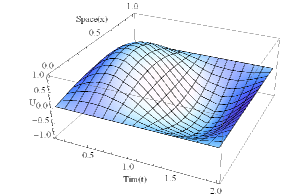
Figure 1: The graph of the solution for Example 1 with $\Gamma(k)=k,N=200$ and k=0.01.

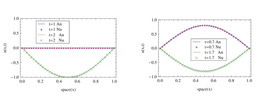
Figure 2: Comparisons between numerical and analytical solutions with $\Gamma(k)=k$ (left) and $\Gamma(k)=2sin(k/2)$ (right) for Example 1 at different times with $N=200,k=0.01$.

Example 2. We consider the hyperbolic telegraph equation (1.1) with $f(x,t)=(3-4\alpha+\beta^{2})\exp(-2t)\sinh(x)$ and the analytical solution $u(x,t)=\exp(-2t)\sinh(x)$ , in the interval $[0,1]$. The boundary conditions and the initial conditions are taken from the exact solution. Tables 4 and 5 give a comparison between the $L_{\infty}$ errors found by our method and the method in [7]. Also Table 5 shows $RMS$ and $L_{2}$ errors. Figure 3, shows absolute error for different values of time with $N=200,k=0.001$.

Table 4: A comparison of $L_{\infty}$ errors of Example 2 for $\alpha=20$, $\beta=10$ at different time and $N=21,k=0.01$.

Method	present method		method in [7]
$Time$	$\Gamma:2sin(\frac{k}{2})$	$\Gamma:k$	Uniform Grid	Nonuniform grid
0.5	2.73131$\times 10^{-6}$	2.59359$\times 10^{-6}$	2.25640$\times 10^{-4}$	2.22066$\times 10^{-4}$
1	1.5714$\times 10^{-6}$	1.48998$\times 10^{-6}$	5.75205$\times 10^{-3}$	1.41294$\times 10^{-4}$
1.5	7.01914$\times 10^{-7}$	6.65254$\times 10^{-7}$	2.43143$\times 10^{-2}$	6.93111$\times 10^{-5}$
2	2.8573$\times 10^{-7}$	2.70754$\times 10^{-7}$	—————–	2.27829$\times 10^{-5}$

Table 5: A comparison of $L_{\infty}$ errors of Example 2 for $\alpha=20$, $\beta=10$ at different time and $N=21,k=0.0001$.

Method	present method		method in [7]
$Time$	$\Gamma:2sin(\frac{k}{2})$	$\Gamma:k$	Uniform Grid	Nonuniform grid
0.5	1.9517$\times 10^{-9}$	1.92002$\times 10^{-9}$	2.23874$\times 10^{-6}$	2.21693$\times 10^{-6}$
1	1.08081$\times 10^{-9}$	1.06278$\times 10^{-9}$	1.72404$\times 10^{-5}$	1.22688$\times 10^{-6}$
1.5	4.75261$\times 10^{-10}$	4.67199$\times 10^{-10}$	4.14630$\times 10^{-3}$	6.73102$\times 10^{-7}$
2	1.91059$\times 10^{-10}$	1.87808$\times 10^{-10}$	—————–	2.66660$\times 10^{-7}$

Table 6: $L_{2}$ and $RMS$ errors of Example 2 for $\alpha=20$, $\beta=10$ at different time and $N=21,k=0.01$.

$\Gamma$	$2sin(\frac{k}{2})$		$k$
$Time$	$L_{2}$	$RMS$	$L_{2}$	$RMS$
0.2	2.36511$\times 10^{-6}$	1.08383$\times 10^{-5}$	2.25651$\times 10^{-6}$	1.03406$\times 10^{-5}$
0.4	2.82003$\times 10^{-6}$	1.2923$\times 10^{-5}$	2.67987$\times 10^{-6}$	1.22807$\times 10^{-5}$
0.8	2.0589$\times 10^{-6}$	9.43506$\times 10^{-6}$	1.95292$\times 10^{-6}$	8.94939$\times 10^{-6}$
1	1.5714$\times 10^{-6}$	7.20105$\times 10^{-6}$	1.48999$\times 10^{-6}$	6.82797$\times 10^{-6}$

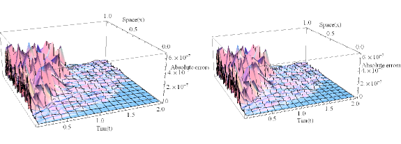
Figure 3: Absolute errors with $\Gamma(k)=k$ (left) and $\Gamma(k)=2sin(k/2)$ (right) for Example 2 with $k=0.001$, $N=200$ and $\alpha=20,\beta=10$.

Example 3. In this example we Consider the hyperbolic telegraph equation (1.1) with $\alpha=10,\beta=5$ in $x\in[0,1]$ and $f(x,t)=-2\alpha\sin(t)\sin(x)+\beta^{2}\cos(t)\cos(x)$. The exact solution for this case is $u(x,t)=\cos(t)\sin(x)$. The boundary conditions and the initial conditions are taken from the exact solution. In order to compare the solutions with [7], we have taken $k=0.001$ and $N=21$. Table 7 gives a comparison between the $L_{\infty}$ error found by our method and by method in [7]. Table 8 shows $L_{2}$ in different partitions. Table 9 shows $RMS$ and $L_{2}$ errors. Figure 4, shows absolute error for different values of time with $N=50,k=0.001$.

Table 7: A comparison of $L_{\infty}$ errors for Example 3 at different time and $N=21,k=0.001$.

Method	present method		method in [7]
$Time$	$\Gamma:2sin(\frac{k}{2})$	$\Gamma:k$	Uniform Grid	Nonuniform grid
0.5	7.59175$\times 10^{-9}$	5.35357$\times 10^{-9}$	1.67216$\times 10^{-5}$	1.28551$\times 10^{-5}$
1	3.5984$\times 10^{-9}$	2.39252$\times 10^{-8}$	4.71302$\times 10^{-4}$	3.20793$\times 10^{-5}$
1.5	1.61922$\times 10^{-8}$	4.2016$\times 10^{-8}$	8.62796$\times 10^{-4}$	5.71454$\times 10^{-5}$
2	2.49884$\times 10^{-8}$	5.20784$\times 10^{-8}$	—————–	6.82827$\times 10^{-5}$

Table 8: A comparison of $L_{2}$ errors of Example 3 at different partitions.

Partitions	N=200,k=0.01		N=400,k=0.001
$Time$	$\Gamma:2sin(\frac{k}{2})$	$\Gamma:k$	$\Gamma:2sin(\frac{k}{2})$	$\Gamma:k$
0.5	3.69769$\times 10^{-8}$	2.46374$\times 10^{-8}$	2.65293$\times 10^{-10}$	1.73258$\times 10^{-10}$
1	1.40829$\times 10^{-8}$	1.16929$\times 10^{-7}$	9.95706$\times 10^{-11}$	8.27160$\times 10^{-10}$
1.5	8.1959$\times 10^{-8}$	2.09527$\times 10^{-7}$	5.80334$\times 10^{-10}$	1.48296$\times 10^{-10}$
2	1.28423$\times 10^{-7}$	2.61864$\times 10^{-7}$	9.09458$\times 10^{-10}$	1.85373$\times 10^{-9}$

Table 9: $L_{2}$ and $RMS$ errors of Example 3 at different time and $N=80,k=0.05$.

$\Gamma$	$2sin(\frac{k}{2})$		$k$
$Time$	$L_{2}$	$RMS$	$L_{2}$	$RMS$
0.5	1.37362$\times 10^{-6}$	1.2286$\times 10^{-5}$	9.94623$\times 10^{-7}$	8.89618$\times 10^{-6}$
1	5.5496$\times 10^{-7}$	4.96372$\times 10^{-6}$	4.61873$\times 10^{-6}$	4.13112$\times 10^{-5}$
1.5	3.22627$\times 10^{-6}$	2.88566$\times 10^{-5}$	8.26127$\times 10^{-6}$	7.38911$\times 10^{-5}$
2	5.05609$\times 10^{-6}$	4.52231$\times 10^{-5}$	1.03189$\times 10^{-5}$	9.22947$\times 10^{-5}$

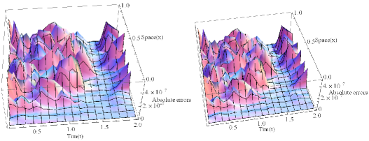
Figure 4: Absolute errors with $\Gamma(k)=k$ (left) and $\Gamma(k)=2sin(k/2)$ (right) for Example 3 with $k=0.001$, $N=50$.

5 Conclusion

The quintic B-spline collocation method is used to solve the one-dimensional hyperbolic telegraph equation with initial and boundary conditions. The convergence analysis of the method is shown. The numerical solutions are compared with the exact solution by finding the RMS ,$L_{2}$ and $L_{\infty}$ errors.The numerical results given in the previous section demonstrate the good accuracy of the scheme proposed in this research.

References

- [1] A. C. Metaxas and R. J. Meredith, Industrial microwave, Heating, Peter Peregrinus, London, 1993.
- [2] J. N. Sharma, Kehar Singh, J. N. Sharma, Partial differential equations for engineers and scientists, second edition, Alpha Science International, 2009.
- [3] G. Roussy and J. A. Pearcy, Foundations and Industrial Applications of Microwaves and Radio Frequency Fields, John Wiley, New York, 1995.
- [4] R.C. Mittal, Rachna Bhatia, A numerical study of two dimensional hyperbolic telegraph equation by modified B-spline differential quadrature method. Appl. Math. Comput 244 (2014) 976-997.
- [5] F. Gao, C. Chi, Unconditionally stable difference schemes for a one-space-dimensional linear hyperbolic equation, Appl. Math. Comput 187 (2007) 1272-1276.
- [6] M. Zarebnia., R. Parvaz, Cubic B-spline collocation method for numerical solution of the one-dimensional hyperbolic telegraph equation, JARSC 4(4) (2012) 46-60.
- [7] R. Jiwari, S. Pandit, R.C. Mittal, A differential quadrature algorithm for solution of the second order one dimensional hyperbolic telegraph equation, IJNS 13 (2012) 259-266.
- [8] H.F. Dinga, Y.X. Zhangb, J.X Caoa, J.H Tianb, A class of difference scheme for solving telegraph equation by new non-polynomial spline methods, Appl. Math. Comput 278 (2012) 4671-4683.
- [9] R.K. Mohanty, M.K. Jain and K. George. On the use of high order difference methods for the system of one space second order nonlinear hyperbolic equations with variable coefficients. J Comput Appl, Math 72(1996)421-431.
- [10] J. Stoer, R. Bulirsch, Introduction to numerical analysis, third edition ,Springer-Verlg, 2002.
- [11] P.M. Prenter, Spline and Variational Methods, Wiley, New York, 1975.
- [12] S.A. Khuri, A. Sayfy, A spline collocation approach for the numerical solution of a generalized nonlinear KleinGordon equation, Appl. Math. Cpmput 216 (2010) 1047-1056.
- [13] G. Pittaluga, L. and Sacripante, Quntic spline interpolation on uniform meshes, Acta. Math. Hung 72 (1996) 4167-175.
- [14] R.K. Mohanty, An unconditionally stable finite difference formula for a linear second order one space dimensional hyperbolic equation with variable coefficients, Appl. Math. Comput 165 (2005) 229-236.