Learning in High-Dimensional Multimedia Data: The State of the Art

Abstract

During the last decade, the deluge of multimedia data has impacted a wide range of research areas, including multimedia retrieval, 3D tracking, database management, data mining, machine learning, social media analysis, medical imaging, and so on. Machine learning is largely involved in multimedia applications of building models for classification and regression tasks etc., and the learning principle consists in designing the models based on the information contained in the multimedia dataset. While many paradigms exist and are widely used in the context of machine learning, most of them suffer from the ‘curse of dimensionality’, which means that some strange phenomena appears when data are represented in a high-dimensional space. Given the high dimensionality and the high complexity of multimedia data, it is important to investigate new machine learning algorithms to facilitate multimedia data analysis. To deal with the impact of high dimensionality, an intuitive way is to reduce the dimensionality. On the other hand, some researchers devoted themselves to designing some effective learning schemes for high-dimensional data. In this survey, we cover feature transformation, feature selection and feature encoding, three approaches fighting the consequences of the curse of dimensionality. Next, we briefly introduce some recent progress of effective learning algorithms. Finally, promising future trends on multimedia learning are envisaged.

1 Introduction

Today, large collections of digital multimedia data are continuously created in different fields and in many application contexts KarpathyCVPR14 ; Feng_2013_ICCV ; ZhuHYSXL13 ; ZhuHSCX12 ; ZhuSS14b . Multimedia finds its applications in various domains including, but not limited to, advertisements, journalism, cultural heritage, animal ecology, Web searching, geographic information systems, ecosystem, surveillance systems, entertainment, medicine, business and social services Choi_2015_CVPR ; DBLP:journals/sigmod/KantorskiMH15 ; DBLP:conf/sigmod/2015 ; GaoSSZS15 ; zhu2015canonical ; zhu2015subspace . The vast amounts of new multimedia data in a large variety of formats (e.g., videos and images) and media modalities (e.g., the combination of, say, text, image, video and sound) are made available worldwide on a daily basis. Moreover, the quantity, complexity, diversity, high dimensionality and multi-modality of these multimedia data are all exponentially growing.

High-dimensional data pose many intrinsic challenges for pattern recognition problems icml11_ngiam ; icml11_yao ; scenecnn_iclr15 ; Gao_2015_CVPR ; DBLP:conf/sigmod/2015 . For example, the curse of dimensionality and the diminishment of specificity in similarities between points in a high dimensional space JMLR:v14:escalante13a ; choi_pami13 ; CVPR14_Khosla . Specifically, the complexity of many existing data mining algorithms is exponential with respect to the number of dimensions. With increasing dimensionality, existing algorithms soon become computationally intractable and therefore inapplicable in many real applications.

An intuitive way is to reduce the number of input variables before a machine learning algorithm can be successfully applied Domingos:2012:FUT:2347736.2347755 ; DBLP:conf/bmvc/ChatfieldLVZ11 ; Wang6751553 ; kantorov2014 . The dimensionality reduction can be made in three different ways to support efficient search and effective storage: 1) feature transformation, which transforms existing high-dimensional features to a new reduced set of features by exploiting the redundancy, noisy or irrelevant of the input data and finding a smaller set of new variables, each being a combination of the input variables, containing basically the same information as the input variables; 2) feature selection, which selects a subset of the existing high-dimensional features by only keeping the most relevant variables from the original dataset; and 3) feature encoding, which encodes the high-dimensional data into a compact code. Alternatively, some machine learning researchers are focusing on the design of efficient machine learning algorithms which can be directly applied to high-dimensional multimedia data.

The organization of the paper is given as follows. Section 2 presents a general framework of learning in high-dimensional multimedia data. Sections 3-5 present some research works on dimensionality reduction, namely feature transformation, feature selection and feature encoding respectively. Section 6 briefly reviews some research efforts on efficient learning schemes for high-dimensional data. Finally, Section 7 provides some promising future trends and concludes this survey.

2 A General Framework for Learning in High-Dimensional Multimedia Data

In this article, we refer to learning in high-dimensional data as: the problem of preprocessing a database of multimedia objects to provide low dimensional data for conventional machine learning algorithms or designing effective machine learning schemes for high dimensional multimedia features.

The general framework of learning in high-dimensional multimedia data is depicted in Fig. 1. Firstly, high-dimensional multimedia features are extracted by using some common feature extraction techniques such as Histogram of Oriented Gradients (HOG), Speeded Up Robust Features (SURF), Local Binary Patterns (LBP), Haar wavelets, and color histograms. After the high-dimensional features are obtained, dimensional reduction techniques are often applied as a data pre-processing step to simplify the data model for computational efficiency and for improving the accuracy of the analysis. The techniques that can be employed for dimension reduction can be partitioned into three categories: 1) feature transformation; 2) feature selection; and 3) feature encoding. The outputs of feature reduction approaches are taken as the inputs for supervised, semi-supervised or unsupervised learning to support multimedia real applications such as multimedia retrieval, multimedia annotation and video tracking Gao_2015_CVPR ; Wang_2015_CVPR ; Shi_2015_CVPR ; Hong_2015_CVPR . Instead of reducing the high-dimensional multimedia data to fit traditional machine learning algorithms, some experts proposed effective learning schemas directly applied to these high-dimensional data to conduct advanced multimedia applicationsNguyen_2015_CVPR ; Papandreou_2015_CVPR ; Zhang_2015_CVPR . In the following sections, we will discuss these techniques in details.

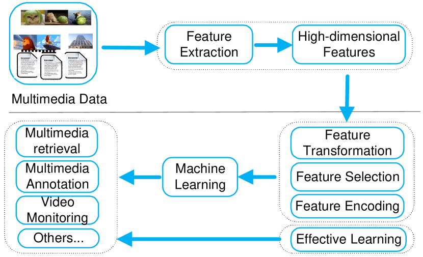
Figure 1: General framework for learning in high-dimensional multimedia data

3 Feature Transformation

Feature transformation is a set of pre-processing techniques that aim to transform the original high-dimensional features to an alternative new set of features (predictor variables), while retaining as much information as possible by dropping less descriptive features from consideration. It has been widely researched in different fields including statistics and machine learning, with applications on object recognition DBLP:conf/eccv/GuptaGAM14 ; DBLP:journals/ijcv/GuptaAGM15 ; ECCV/2012/Ali , data analysis and visualizations Saini:2012:MOM:2393347.2393373 , and many others Maaten2009 ; DBLP:conf/vluds/EngelHH11 .

Following DBLP:conf/vluds/EngelHH11 , feature transformation can be generally formulated as below. Let ${X}\in\mathbb{R}^{m\times n}$, a set of $n$ data points in an $m$-dimensional feature space, and two distance (or dissimilarity) functions, ${d_{m}}:\mathbb{R}^{m}\times\mathbb{R}^{m}\to\mathbb{R}$’ and ${d_{t}:\mathbb{R}^{t}\times\mathbb{R}^{t}\to\mathbb{R}}$’, over the $m$-dimensional data space and the target $’t$-dimensional subspace respectively, with $t\ll m$. A mapping function $\phi$ that maps the $m$-dimensional data points $({x}_{i}\in{X})$ to the $t$-dimensional target points $({y}_{i}\in{Y})$, i.e.,

$$\phi:\mathbb{R}^{m}\to\mathbb{R}^{t},{x}_{i}\to{y}_{i},1\leq i\leq n$$ (1)

is defined s.t. $\phi$ “faithfully” approximates pairwise distance relationships of ${X}$ by those of ${Y}\in\mathbb{R}^{t\times n}$, thereby mapping close (similar) points in data space to equally close points in target space, i.e., $d_{m}({x}_{i},{x}_{j})\approx d_{t}({y}_{i},{y}_{j})$, for $1\leq i,j\leq n$. In particular, an adequate mapping is designed to ensure that remote data points are mapped to remote target points. Since the target space usually has lower degrees of freedom than those required to model distance relationships in the original space, the mapping $\phi$ adheres to an inherent error that is to be minimized by its definition. Thereby, $\phi$ is commonly defined to minimize the least squares error:

$${\varepsilon_{\phi}}\!=\!\sum\nolimits_{{1}\leq i,j\leq n}{{{M}_{i,j}}{{\left({{d_{m}}\left({{\mathbf{x}_{i}},{{x}_{j}}}\right)\!-\!{d_{t}}\left({{{y}_{i}},{{y}_{j}}}\right)}\right)}^{2}}},{M}\!\in\!\mathbb{R}^{n\times n}$$

where ${M}$ is a matrix used to define the weights of certain data relationships or dimensions. Beside pairwise distance relationship preservation, there are also some variants on $\phi$ which are designed to preserve other relationships, such as the nearest neighbors relationship, or to minimize the errors measured by other factors depending on the distance functions used.

Feature transformation can be roughly categorized into linear transformation and non-linear transformation. For linear transformation, an explicit linear transformation function is learned to reduce the dimensionality and increase the robustness and the performance of domain applications. As one of the first dimension reduction techniques discussed in the literature, Principal Components Analysis (PCA) jolliffe2002principal conveys distance relationships of the data by orthogonally projecting it on a linear subspace of target dimensionality. In this specific subspace, the orthogonally projected data has maximal variance. Latent Semantic Analysis (LSA) is a variant on the PCA idea presented in DeerwesterDLFH90 and it has been employed on documents, images, videos and musics He03 . Linear discriminant analysis (LDA) hastie01statisticallearning is a supervised subspace learning method which is based on Fisher Criterion. It aims to find a linear transformation $W\in\mathbb{R}^{d\times m}$ that maps $x_{i}$ in the d-dimensional space to a m-dimensional space, in which the between class scatter is maximized while the within-class scatter is minimized. LDR cunningham2015ldr interprets linear dimensionality reduction in a simple optimization framework as a program with a problem-specific objective over orthogonal or unconstrained matrices. This framework gives insight to some rarely discussed shortcomings of well-known methods and further allows straightforward generalizations and novel variants of classical methods.

Linear transformation would be considered as a shortcoming in many applications and lots of research efforts have been devoted to non-linear feature transformation. Multidimensional Scaling (MDS) LafonL06 , also known as classical MDS, is a well-established approach that uses projection to map high-dimensional points to a linear subspace of lower dimensionality. The technique is often motivated by its goal to preserve pairwise distances in this mapping. As such, MDS defines a faithful approximation as one that captures pairwise distance relationships in an optimal way; more precisely, inner product relations. MDS has proven to be successful in many applications, but it suffers from the fact that it is based on Euclidean distances, and does not take into account the distribution of the neighboring datapoints. Isomap TengLFCS05 is a technique that resolves this problem by attempting to preserve pairwise geodesic (or curvilinear) distances between datapoints. Geodesic distance is the distance between two points measured over the manifold. In Isomap, the geodesic distances between the datapoints $x_{i}\leavevmode\nobreak\ (i\in\{1,2,...,n\})$ are computed by constructing a neighborhood graph $G$, in which every datapoint $x_{i}$ is connected with its $k$ nearest neighbors. The shortest path between two points in the graph forms a good estimate of the geodesic distance between these two points, and can easily be computed using shortest-path algorithms. The low-dimensional representations $y_{i}$ of the datapoints $x_{i}$ in the low-dimensional space $Y$ are computed by applying multidimensional scaling on the resulting distance matrix. In Wichterich:2008:EES:1376616.1376639 , a method designed for Earth Mover’s Distance (EMD) is proposed to increase efficiency in the search process. It incorporates EMD assignment analysis among dimensions to obtain effective reduction. A tight EMD bound in the subspace is established to generate only a small number of candidates for the expensive EMD computations in the original space. Local Linear Embedding (LLE) saul06spectral is a local technique for dimensionality reduction that is similar to Isomap in that it constructs a graph representation of the datapoints. In contrast to Isomap, it attempts to preserve solely local properties of the data. LLE describes the local properties of the manifold around a datapoint $x_{i}$ by writing the datapoint as a linear combination $W_{i}$ (the so-called reconstruction weights) of its k nearest neighbors $x_{ij}$. Hence, LLE fits a hyperplane through the datapoint $x_{i}$ and its nearest neighbors, thereby assuming that the manifold is locally linear. Based on this weighted matrix, the low-dimensional space $Y$ can be computed. Some other non-linear feature transformation methods include kernel PCA 0026002 , Hessian LLE citeulike:905977 , Laplacian Eigenmaps BelkinN03 , LTSA ZhangZ04 and so on.

More recently, deep learning LeeEN07 ; WangHWW14 ; RifaiVMGB11 have achieved great success for dimensionality reduction via the powerful representability of neural networks. A few algorithms that work well for this purpose, beginning with restricted Boltzmann machines (RBMs) hinton2006reducing and autoencoders BengioLPL06 . In GAE WangHWW14 , they extend the traditional autoencoder and propose a dimensionality reduction method by manifold learning, which iteratively explores data relation and use the relation to pursue the manifold structure. In CAE RifaiVMGB11 , they add a well chosen penalty term to the classical reconstruction cost function and achieve results that equal or surpass those attained by other regularized autoencoders as well as denoising auto-encoders VincentLLBM10 on a range of datasets.

4 Feature Selection

Feature selection methods provide us a way of reducing computation time, improving prediction performance, and a better understanding of the data in machine learning He6247966 ; icml2014c2_jawanpuria14 ; cvpr2013bbprbm . The focus of feature selection is to select a subset of variables from the input which can efficiently describe the input data while reducing effects from noise or irrelevant variables and still provide good prediction results GuyonE03 ; icml2013pgbm ; icassp2013deepemotion . It can be broadly classified into two categories: 1) filter methods, which aim to remove irrelevant features from the original high-dimensional features or identify the most relevant subset features for maximally describing the information of the original information; and 2) wrapper methods, which choose a set of relevant features by searching through the feature space and then selecting the candidate feature subsets for supporting the highest predictor performance.

4.1 Filter Methods

Filter methods use variable ranking techniques as the principle criteria for variable selection by ordering Kourosh2008 . The most popular filter strategies for feature selection include Information gain Reunanen03 , Chi-square measure wu2002feature , the Laplacian score (LS) He03 , odds ratio Mladenic98 and its derivatives HeCN05 . Ranking methods are used due to their simplicity and good performance is reported for practical applications. A suitable ranking criterion is used to score the variables and a threshold is used to eliminate variables below the threshold. Ranking methods are filter methods since they are applied before classification to filter out the less relevant variables. A basic property of a good feature is to contain useful information about the different classes in the data. This property can be defined as the feature relevance which provides a measurement of the discrimination power of a feature to different classes Kohavi97wrappersfor . Several publications HeCN05 ; Reunanen03 have presented various definitions and measurements for the relevance of a variable.

Next we look into two representative ranking methods. The input data $[x_{ij},y_{i}]$ consists of $n$ samples $i=1$ to $n$ with $m$ variables $j=1$ to $m$, $x_{i}$ is the $i$th sample and $y_{i}$ is the class label for $x_{i}$.

A widely used criteria is the correlation criteria, which can be defined as:

$$R\left(i\right)={{{\mathop{cov}}\left({{x_{i}},Y}\right)}}/{{\sqrt{{\mathop{var}}\left({{x_{i}}}\right)\times{\mathop{var}}\left(Y\right)}}}$$ (2)

where $x_{i}$ is the $i$-th variable, $Y$ is the output (class labels), $cov()$ is the covariance and $var()$ the variance. Note that correlation ranking can only detect linear dependencies between variable and target.

Information theoretic ranking criteria uses the measure of dependency (mutual information) between two variables. It is based on the observation that if one variable can provide information about the other then they are dependent. We start with Shannons definition for entropy given by:

$$H\left(Y\right)=-\sum\nolimits_{y}{p\left(y\right)\log\left({p\left(y\right)}\right)}$$ (3)

It represents the uncertainty (information content) in the output $Y$. Suppose we observe a variable $X$ then the conditional entropy is given by:

$$H\left({Y|X}\right)=-\sum\nolimits_{x,y}{p\left({x,y}\right)\log\left({p\left({y|x}\right)}\right)}$$ (4)

It implies that by observing a variable X, the uncertainty in the output Y. The decrease in uncertainty is given as:

$$I\left({Y,X}\right)=H\left(Y\right)-H\left({Y|X}\right)$$ (5)

This gives the mutual information between $Y$ and $X$ meaning that if $X$ and $Y$ are independent then mutual information will be zero and greater than zero if they are dependent. The definitions provided above are given for discrete variables and the same can be obtained for continuous variables by replacing the summations with integrations.

Recently, lots of research efforts have be devoted to filter-based feature selection. In JavedBS12 ; RehmanJBS15 the authors develop a ranking criteria based on class densities for binary data. A two stage algorithm utilizing a less expensive filter method to rank the features and an expensive wrapper method to further eliminate irrelevant variables is used. The advantages of feature ranking are that it is computationally light and it avoids overfitting and is proven to work well for certain datasets LazarTMSCMSDBN12 ; GuyonE03 . Filter methods do not rely on learning algorithms which are biased. This is equivalent to changing data to fit the learning algorithm. One of the drawbacks of ranking methods is that the selected subset might not be optimal in that a redundant subset might be obtained. Some ranking methods such as Pearson correlation criteria and MI do not discriminate the variables in terms of the correlation to other variables. The variables in the subset can be highly correlated in that a smaller subset would suffice Chandrashekar201416 . In feature ranking, important features that are less informative on their own but are informative when combined with others could be discarded GuyonE03 . Finding a suitable learning algorithm can also become hard since the underlying learning algorithm is ignored.

4.2 Wrapper Methods

Wrapper methods use the predictor as a black box and the predictor performance as the objective function to evaluate the variable subset. Since evaluating 2N subsets becomes a NP-hard problem, suboptimal subsets are found by employing search algorithms which find a subset heuristically. A number of search algorithms can be used to find a subset of variables which maximizes the objective function. We broadly classify the wrapper methods into Sequential Selection Algorithms (SSA) and Heuristic Search Algorithms (HSA). The SSA start with an empty set and add features until the maximum objective function is obtained, while the HSA evaluate different subsets to optimize the objective function.

For SSA, Two representative methods are Sequential Feature Selection (SFS) and Sequential Floating Forward Selection (SFFS). The SFS algorithm Pudil:1994 starts with an empty set and adds one feature for the first step which gives the highest value for the objective function. Next, the remaining features are added individually to the current subset and the new subset is evaluated. While SFFS Reunanen03 algorithm is more flexible than the naive SFS because it introduces an additional backtracking step. Specifically, the first step of the SFFS is the same as the SFS. Next, the SFFS excludes one feature at a time from the subset obtained in the first step and evaluates the new subsets. If excluding a feature increases the value of the objective function then that feature is removed and goes back to the first step with the new reduced subset or else the algorithm is repeated from the top. This process is repeated until the required number of features are added or the required performance is reached.

For HSA, Genetic Algorithm (GA) Goldberg:1989:GAS:534133 can be used to find a subset of features where in the chromosome bits represent if the feature is included or not. The global maximum for the objective function can be found which gives the best suboptimal subset. Here again the objective function is the predictor performance. The GA parameters and operators can be modified within the general idea of an evolutionary algorithm to suit the data or the application to obtain the best performance or the best search results. Multi-objective GA is used for hand written digit recognition in OliveiraSBS03 .

5 Feature Encoding

Feature encoding methods encode the high-dimensional data into compact codes so that efficient retrieval and effective storing can be conducted.

5.1 Quantization

The general quantization problem can be formulated as $\zeta:{x}\in\mathbb{R}^{m}\longrightarrow\{0,1,...,2^{L}\}$, where $\zeta$ is the function to quantize an $m$-dimensional feature vector $x$ to a value in $\{0,1,...,2^{L}\}$ and $L$ is the number of bits for approximating the $m$-dimensional feature vectors. For the special case of $m$=1 (called scalar quantization), a scalar input is provided, and it implies that a range of scalar quantities are quantized into a single integer (or the same bit-string). For the cases of $m>1$ (called vector quantization), it means that a group of vectors are approximated into the same bit-string.

5.1.1 Scalar Quantization

Scalar quantization takes a real-valued scalar quantity and maps it into one of a finite set of values. The idea of using quantization for high-dimensional indexing to overcome the “dimensionality curse” first appeared in DBLP:conf/vldb/WeberSB98 , where a very simple scalar quantization scheme called Vector-Approximation file (VA-file) is proposed. For each dimension $i$, the VA-file partitions the one-dimensional data range into $2^{L_{i}}$ slices where $L_{i}$ is the number of bits for representing the dimension. Each dimension can then be approximated by $L_{i}$ bits by checking to which slice the value on dimension $i$ belongs (i.e., map the value into one of 0 to $2^{L_{i}}$-1). Given an $m$-dimensional feature vector, a bit-string of length $L=\sum L_{i}$ by concatenating all its dimensions’ bits is used to approximate the original feature vector.

5.1.2 Vector Quantization

Vector quantization works by dividing all the feature vectors into groups (or clusters). It takes a feature vector and then maps it into one of the finite set of groups, where each group is approximated by its centroid point. Depending on the number of groups needed, different numbers of bits $b$ can be determined to encode the group IDs. An example of vector quantization is the $K$-means clustering. Formally, the standard $K$-means clustering is defined as below Lloyd82 .

Given $N$ feature vectors ${X}=\{{x}_{1},\cdots,{{x}}_{n}\}\in\mathbb{R}^{m\times n}$, the $K$-means algorithm partitions the database into $K$ clusters, each of which associates one codeword ${{c}}_{i}\in\mathbb{R}^{m\times 1}$. Let ${{C}}=[{{c}}_{1},\cdots,{{c}}_{K}]\in\mathbb{R}^{m\times K}$ be the corresponding codebook. Then the codebook is learned by minimizing the within-cluster distortion, e.g.,

$$\min\leavevmode\nobreak\ \leavevmode\nobreak\ {\sum_{i}{\|{{x}}_{i}-{{C}}{{v}}_{i}\|_{2}^{2}}}$$ (6)

$$\operatorname{s.t.}\leavevmode\nobreak\ \leavevmode\nobreak\ {{v}}_{i}\in\{0,1\}^{K\times 1},\forall i,\|{{v}}_{i}\|_{1}=1,\forall i$$

where ${{v}}_{i}$ is a $1$-of-$K$ encoding vector (i.e., $K$ dimensions with one $1$ and $(K-1)$ $0$s) to indicate which codeword is used to map ${{x}}_{i}$, and $\|\cdot\|_{1}$ is the $\ell_{1}$ norm.

In vector quantization, vectors are quantized into clusters. Given a query vector, it is firstly mapped into the closest clusters, followed by computing the distances between the query vector and all the feature vectors inside those clusters. For large-scale high-dimensional databases, it is very challenging to determine the value of $K$. When $K$ is too small, coarse quantization is performed, i.e., too many vectors are approximated into the same cluster, leading to many database vectors to be accessed and compared. Although a larger $K$ value results in finer quantization, consequently more clusters need to be accessed to search the closest ones. To maintain high-quality quantization, large $K$ values are usually required. To index a large number of clusters, they can be hierarchically organized in a vocabulary tree which directly defines the vector quantization DBLP:conf/cvpr/NisterS06 . The quantization and the indexing can then be integrated. Naturally, it also inherits the drawbacks of tree structures to a certain degree.

5.1.3 Product Quantization

Scalar quantization quantizes each dimension of the vector and may over-quantize the data since each dimension may require multiple bits. On the contrary, vector quantization quantizes the full-dimensional vectors as a whole and may under-quantize the data since each vector needs a few bits only, independent of the dimensionality. Scalar quantization suffers from scanning relatively large-sized approximations, while vector quantization has the scalablity issue when comparing a large number of clusters. To address these problems, product quantization (PQ) DBLP:journals/pami/JegouDS11 is proposed to perform quantization on subvectors of the original full-dimensional vectors, i.e., an intermediate of scalar quantization and vector quantization.

The key idea of PQ is to split an $m$-dimensional vector into $P$ disjoint subvectors on which quantization is then performed. Assume the $j$-th subvector contains $m_{j}$ dimensions and then $m=\sum_{j=1}^{P}{m_{j}}$. Without loss of generality, $m_{j}$ is set to $m/P$ and $m$ is assumed to be divisible by $P$. For each subvector, $K$-means is performed on all the database vectors to obtain $K$ sub codewords. With $K\times P$ clusters generated from $P$ subvectors, it can have the capacity to represent $K^{P}$ possible clusters on the original $m$-dimensional vector space based on the Cartesian product relationship among subvectors.

Let ${{C}}^{j}\in\mathbb{R}^{m_{j}\times K}$ be the matrix of the $j$-th sub codebook and each column is an $m_{j}$-dimensional sub codeword. As discussed in NorouziF13 ; WangWSXSL15 , PQ can be taken as optimizing the following problem with respect to ${{C}}^{j}$ and ${{v}}_{i}^{j}$, where ${{v}}_{i}^{j}$ is the 1-of-$K$ encoding vector on the $j$-th subvector and the index of $1$ indicates which sub codeword is used to encode the $j$-th subvector for the $i$-th vector ${{x}}_{i}$:

$$\begin{split}\min\leavevmode\nobreak\ \leavevmode\nobreak\ f_{\text{PQ},P,K}=\sum_{i}{\left\|{{x}}_{i}-\begin{bmatrix}{{C}}^{1}{{v}}_{i}^{1}\\ \vdots\\ {{C}}^{P}{{v}}_{i}^{P}\end{bmatrix}\right\|_{2}^{2}}\\ \operatorname{s.t.}\leavevmode\nobreak\ \leavevmode\nobreak\ {{v}}_{i}^{j}\in\{0,1\}^{K\times 1},\forall i,j,\|{{v}}_{i}^{j}\|_{1}=1,\forall i,j.\end{split}$$ (7)

The main advantage of PQ lies in the fact that only a very small number of clusters generated from subvectors are used to approximate the full Euclidean distance. Therefore, the required memory cost is small. To avoid an exhaustive scan on the database codes, an inverted file is also combined to index clusters. Given a query, the inverted file is first accessed to limit the search space, then more accurate Euclidean distances can be computed based on the subvector-to-centroid distances.

5.2 Hashing

Very recently, hashing ZhuHSZ13 ; ZhuZH14 ; ZhuHCCS13 ; song2013effective ; ZouCSZYS15 ; MM15zou ; MM15song ; MM15gao ; ZouLLFYL13 ; ZouFLLYLL13 has attracted enormous attention from different research areas to achieve fast similarity search due to its high efficiency in terms of the storage and computational cost. The basic idea of hashing is to encode a high-dimensional data point (or feature vector) into a binary code (i.e., a bit-string). Different from quantization, for two binary codes in hashing, their Hamming distance in the Hamming space can be directly employed to measure the closeness between two corresponding high-dimensional feature vectors. Compared with distances computed on real-valued high-dimensional feature vectors, the Hamming distance computed on binary codes is far more efficient by using bit operations. The form of hashing can be formulated as below: $\mathbf{y}={\mathcal{H}}({x})\in\{0,1\}^{L},$ where ${{x}}$ is an $m$-dimensional real-valued vector, $\mathbf{y}$ is the corresponding binary code for ${x}$ with $L$ bits, and $\mathcal{H}$ is the hash function family to map ${x}$ into $\mathbf{y}$. Typically, in the hash function family, one hash function is used to generate one bit of the binary code, i.e., $\mathcal{H}({x})=({h}_{1}({x}),\cdots,{h}_{L}({x})).$

The most challenging problem on hashing is how to generate effective hash functions which can perform approximate similarity search as accurately as possible. In other words, hashing functions should preserve the similarity relationship among feature vectors from the original high-dimensional feature space to the mapped Hamming space. According to the characteristics of training data, they can be summarized into unsupervised hashing, supervised hashing, and semi-supervised hashing.

For unsupervised hashing where training data have no labels, many works exploit the low energy spectrum of data neighborhood graphs to obtain the hash codes and hash functions Weiss08 ; DBLP:conf/icml/LiuWKC11 . This group of methods usually requires building a neighborhood graph and computing eigenvalues of this graph Laplacian. An alternative solution is to seek principled linear projections using PCA DBLP:journals/pami/WangKC12 or sparse coding ZhuHCCS13 .

While unsupervised hashing shows promise in retrieving neighbors based on metric distances, e.g., $\ell_{2}$ distance, a variety of practical applications prefer semantically similar neighbors SHCVPR2008 . Therefore, some recent works have also incorporated supervised information to improve the hashing performance. Such supervised information can be customarily expressed as labels of similar (or relevant) and dissimilar (or irrelevant) data pairs when available. Typical supervised hashing methods include Semantic Hashing salakhutdinov2007semantic , Minimal Loss Hashing (MLH) DBLP:conf/icml/NorouziF11 , Linear Discriminant Analysis Hashing (LDAHash) strecha2012ldahash , Kernelized Supervised Hashing (KSH) DBLP:conf/cvpr/LiuWJJC12 , Order Preserving Hashing (OPH) Wangjianfeng13 , etc. Supervised hashing is expected to achieve better result quality than unsupervised hashing, if the supervised information is properly utilized.

One of the main problems with supervised hashing methods is that very noisy or limited training data may easily lead them to be ineffective or over-fitting. To tackle this problem, Semi-Supervised Hashing (SSH) has also been studied DBLP:journals/pami/WangKC12 . SSH aims to minimize the empirical errors on the labeled training data. At the same time, it also maximizes the variance and the independence of different bits on both the labeled data and the unlabeled data. Lai et al.Lai_2015_CVPR proposed a ”one-stage” supervised hashing method via a deep architecture that maps input images to binary codes. The proposed deep architecture uses a triplet ranking loss designed to preserve relative similarities. Semantics Preserving Hashing (SePH) Lin_2015_CVPR method is proposed for cross-view retrieval. It utilizes kernel logistic regression with a sampling strategy as basic hash functions to model the projections from features in each view to the hash codes. Hashing across Euclidean space and Riemannian manifold (HER) is proposed by deriving a unified framework to firstly embed the two spaces into corresponding reproducing kernel Hilbert spaces, and then iteratively optimize the intra- and inter-space Hamming distances in a maxmargin framework to learn the hash functions for the two spaces Lin_2015_CVPR . Table 1 shows the comparative results of some standard hashing methods in precision on the ILSVRC 2012 dataset.

Table 1: Comparative results in precision of Hamming distance on the ILSVRC 2012 datase(10,000 samples are used for training).

Method	64 bits	128 bits
BRE NIPS2009_3667	High	low
SSH DBLP:journals/pami/WangKC12	low	low
ITQ DBLP:journals/pami/GongLGP13	fair	fair
KSH DBLP:conf/cvpr/2012	High	fair
FastHash DBLP:journals/corr/LinSSHS14	High	High
Dataset	Dim	Reference Set
MNIST	784	60K
SIFT10K	128	10K
SIFT1M	128	1M
GIST1M	960	1M
Tiny1M	384	1M
SIFT1B	128	1B

There are also some further developments extended from the standard hashing algorithms: Multiple Feature Hashing (MFH) DBLP:conf/mm/SongYHSH11 learns a group of hash functions to generate binary codes for multiple visual features generated from the same media type, e.g., videos. Cross-Media Hashing Kumar:2011:LHF:2283516.2283623 ; DBLP:conf/sigmod/SongYYHS13 ; DBLP:conf/kdd/ZhenY12 considers different media types of data from heterogeneous data sources (e.g., text documents from Google and images from Facebook) to support cross-media retrieval and jointly feeds them into the same model for efficient hashing. Complementary Hashing XuWLZLY11 employs multiple complementary hash tables to further improve the search quality. It balances the recall and the precision in a more effective way. Weighted Hamming Distance (WHD) zhang2013 has been proposed to rank the binary codes of hashing methods to improve the ranking quality based on the Hamming distance. Moreover, robust hashing with local modes (RHLM) 6714849 for accurate and fast approximate similarity search have been proposed. Specifically, it uses the learned hash functions, and all the database points are then mapped into their binary hash codes and organized into buckets. Data points having the same hash code belong to a single bucket that is identified by the hash code. Given a query data point, approximate similarity search can be efficiently achieved by exploring the buckets, which have similar hash codes to the query hash code. A comparison with the state-of-the art single modality and multiple modalities hash learning methods is shown in Lin_2015_CVPR .

6 Effective Learning Schemes

While dimensional reduction is a possible way to alleviate the effect of high-dimensionality, some effective learning schemes are proposed for online learning and paralleling computing to directly deal with the high-dimensional data.

Online learning Shalev-Shwartz12 is a well established learning paradigm which has both theoretical and practical appeals. The key difference between online learning and batch learning techniques, is that in online learning the mapping is updated after the arrival of every new data point in a scalable fashion, while batch techniques are used when one has access to the entire training dataset at once. Therefore, online learning is able to deal with scalable and high-dimensional data. Online learning has been studied in several research fields including game theory, information theory and machine learning mcmahan2011follow ; BartlettHR07 .

Online learning is performed in a sequence of consecutive rounds, where at round t the learner is given a question, $x_{t}$, taken from an instance domain $X$ , and is required to provide an answer to this question, which we denote by $p_{t}$. After predicting an answer, the correct answer, $y_{t}$, taken from a target domain $Y$, is revealed and the learner suffers a loss, $l(p_{t},y_{t})$, which measures the discrepancy between his answer and the correct one. While in many cases $p_{t}$ is in $Y$, it is sometimes convenient to allow the learner to pick a prediction from a larger set, which we denote by $D$. Many successful algorithms have been developed over the past few years to optimize the online learning problem, and they differ in the choice of loss function and regularization term. A modern view of these algorithms casts the problem as the task of following the regularized leader (FTRL) mcmahan2011follow . Informally, FTRL methods choose the best decision in hindsight at every iteration. Verbatim usage of the FTRL approach fails to achieve low regret, however, adding a proximal term to the past predictions leads to numerous low regret algorithms HazanK10 . The proximal term strongly affects the performance of the learning algorithm. Therefore, adapting the proximal function to the characteristics of the problem at hand is desirable. Online gradient descent BartlettHR07 generalizes this FTRL by deriving a simple reduction from convex functions to linear functions. In DuchiHS10 , the authors present a new family of sub-gradient methods that dynamically incorporate knowledge of the geometry of the data observed in earlier iterations to perform more informative gradient based learning. Mirror descent BartlettHR07 generalizes online gradient descent, and considers the best-experts problem, where on each round we must choose an ‘expert’ from a set whose advice we follow for that round.

The high-dimensional and big data phenomenon is intrinsically related to the paralleling computing. Large companies as Facebook, Yahoo!, Twitter, LinkedIn benefit and contribute working on paralleling computing projects. Big Data infrastructure deals with Hadoop, and other related software as: 1) Apache Hadoop, a software for data-intensive distributed applications, based in the MapReduce programming model and a distributed file system called Hadoop Distributed Filesystem (HDFS). Hadoop allows writing applications that rapidly process large amounts of data in parallel on large clusters of compute nodes. A MapReduce job divides the input dataset into independent subsets that are processed by map tasks in parallel. This step of mapping is then followed by a step of reducing tasks. These reduce tasks use the output of the maps to obtain the final result of the job. 2) Apache S4 NeumeyerRNK10 : platform for processing continuous data streams. S4 is designed specifically for managing data streams. S4 apps are designed combining streams and processing elements in real time.

7 Future Trends and Conclusion

Hign-dimensionality and big data is going to continue growing during the next years, especially with the emergence of deep learning and social media. The data is going to be more diverse, larger, and complex. Therefore, dimension reduction algorithms are still going to be a hot research topic in the near future. On the other hand, effect learning algorithms for first-order optimization, online learning and paralleling computing will be more desired.

We discussed in this paper some insights about the learning in high-dimensional data. We first consider the main challenges for the high-dimensional data and then survey some existing techniques dealing with the problem. Finally, we conclude this paper by providing some possible future trends.

8 Acknowledge

The work of Lianli Gao has been partially supported by NSFC (Grant No.61502080) and by the Fundamental Research Funds for the Central University (Grant No.ZYGX2014J063). The work of Junming Shao has been supported partially by NSFC (Grant No. 61403062, 61433014), and Fundamental Research Funds for the Central Universities (Grant No. ZYGX2014J053).

References

- (1) Peter L. Bartlett, Elad Hazan, and Alexander Rakhlin. Adaptive online gradient descent. In NIPS, 2007.
- (2) Mikhail Belkin and Partha Niyogi. Laplacian eigenmaps for dimensionality reduction and data representation. Neural Computation, 15(6):1373–1396, 2003.
- (3) Yoshua Bengio, Pascal Lamblin, Dan Popovici, and Hugo Larochelle. Greedy layer-wise training of deep networks. In NIPS, pages 153–160, 2006.
- (4) Ali Borji, Ming-Ming Cheng, Huaizu Jiang, and Jia Li. Salient object detection: A benchmark. CoRR, abs/1501.02741, 2015.
- (5) Girish Chandrashekar and Ferat Sahin. A survey on feature selection methods. Computers and Electrical Engineering, 40(1):16–28, 2014.
- (6) Ken Chatfield, Victor S. Lempitsky, Andrea Vedaldi, and Andrew Zisserman. The devil is in the details: an evaluation of recent feature encoding methods. In BMVC, pages 1–12, 2011.
- (7) Sungjoon Choi, Qian-Yi Zhou, and Vladlen Koltun. Robust reconstruction of indoor scenes. In CVPR, June 2015.
- (8) Wongun Choi, Caroline Pantofaru, and Silvio Savarese. A general framework for tracking multiple people from a moving camera. TPAMI, 35(7):1577–1591, 2013.
- (9) J.P. Cunningham and Z. Ghahramani. Linear dimensionality reduction: survey, insights, and generalizations. JMLR, 2015.
- (10) Luiz E. Soares de Oliveira, Robert Sabourin, Flávio Bortolozzi, and Ching Y. Suen. A methodology for feature selection using multiobjective genetic algorithms for handwritten digit string recognition. In IJPRAI, 2003.
- (11) Scott C. Deerwester, Susan T. Dumais, Thomas K. Landauer, George W. Furnas, and Richard A. Harshman. Indexing by latent semantic analysis. JASIS, 41(6):391–407, 1990.
- (12) LJP Van der Maaten, EO Postma, and HJ Van den Herik. Dimensionality reduction: A comparative review. In Technical Report TiCC TR 2009-005, 2009.
- (13) Pedro Domingos. A few useful things to know about machine learning. Commun. ACM, 55(10):78–87, 2012.
- (14) David L. Donoho and Carrie Grimes. Hessian eigenmaps: Locally linear embedding techniques for high-dimensional data. Proceedings of the National Academy of Sciences of the United States of America, 100(10):5591–5596, 2003.
- (15) John C. Duchi, Elad Hazan, and Yoram Singer. Adaptive subgradient methods for online learning and stochastic optimization. JMLR, 12:2121–2159, 2011.
- (16) Daniel Engel, Lars Hüttenberger, and Bernd Hamann. A survey of dimension reduction methods for high-dimensional data analysis and visualization. In VLUDS, pages 135–149, 2011.
- (17) Alberto N. Escalante-B. and Laurenz Wiskott. How to solve classification and regression problems on high-dimensional data with a supervised extension of slow feature analysis. JMLR, 14:3683–3719, 2013.
- (18) Zheyun Feng, Rong Jin, and Anil Jain. Large-scale image annotation by efficient and robust kernel metric learning. In ICCV, December 2013.
- (19) Lianli Gao, Jingkuan Song, Feiping Nie, Yan Yan, Nicu Sebe, and Heng Tao Shen. Optimal graph leaning with partial tags and multiple features for image and video annotation. In CVPR, 2015.
- (20) LianLi Gao, Jingkuan Song, Junming Shao, Xiaofeng Zhu, and Heng Tao Shen. Zero-shot image categorization by image correlation exploration. In ICMR, pages 487–490, 2015.
- (21) Lianli Gao, Jingkuan Song, Fuhao Zou, Dongxiang Zhang, and Jie Shao. Scalable multimedia retrieval by deep learning hashing with relative similarity learning. In ACM Multimedia, 2015.
- (22) David E. Goldberg. Genetic Algorithms in Search, Optimization and Machine Learning. Addison-Wesley Longman Publishing Co., Inc., 1st edition, 1989.
- (23) Yunchao Gong, Svetlana Lazebnik, Albert Gordo, and Florent Perronnin. Iterative quantization: A procrustean approach to learning binary codes for large-scale image retrieval. TPAMI, 35(12):2916–2929, 2013.
- (24) Saurabh Gupta, Pablo Andrés Arbeláez, Ross B. Girshick, and Jitendra Malik. Indoor scene understanding with RGB-D images: Bottom-up segmentation, object detection and semantic segmentation. IJCV, 112(2):133–149, 2015.
- (25) Saurabh Gupta, Ross B. Girshick, Pablo Andrés Arbeláez, and Jitendra Malik. Learning rich features from RGB-D images for object detection and segmentation. In ECCV, pages 345–360, 2014.
- (26) Isabelle Guyon and André Elisseeff. An introduction to variable and feature selection. JMLR, 3:1157–1182, 2003.
- (27) Trevor Hastie, Robert Tibshirani, and Jerome Friedman. The Elements of Statistical Learning. Springer New York Inc., 2001.
- (28) Elad Hazan and Satyen Kale. Extracting certainty from uncertainty: regret bounded by variation in costs. Machine Learning, 80(2-3):165–188, 2010.
- (29) Ran He, Tieniu Tan, Liang Wang, and Wei-Shi Zheng. l2, 1 regularized correntropy for robust feature selection. In CVPR, pages 2504–2511, June 2012.
- (30) Xiaofei He, Deng Cai, and Partha Niyogi. Laplacian score for feature selection. In NIPS, 2005.
- (31) Xiaofei He and Partha Niyogi. Locality preserving projections. In NIPS, 2003.
- (32) Geoffrey E Hinton and Ruslan R Salakhutdinov. Reducing the dimensionality of data with neural networks. Science, 313(5786):504–507, 2006.
- (33) Zhibin Hong, Zhe Chen, Chaohui Wang, Xue Mei, Danil Prokhorov, and Dacheng Tao. Multi-store tracker (muster): A cognitive psychology inspired approach to object tracking. In CVPR, 2015.
- (34) Kashif Javed, Haroon Atique Babri, and Mehreen Saeed. Feature selection based on class-dependent densities for high-dimensional binary data. TKDE, 24(3):465–477, 2012.
- (35) Pratik Jawanpuria, Manik Varma, and Saketha Nath. On p-norm path following in multiple kernel learning for non-linear feature selection. In ICML, pages 118–126, 2014.
- (36) Hervé Jégou, Matthijs Douze, and Cordelia Schmid. Product quantization for nearest neighbor search. TPAMI, 33(1):117–128, 2011.
- (37) Ian Jolliffe. Principal component analysis. Wiley Online Library, 2002.
- (38) V. Kantorov and I. Laptev. Efficient feature extraction, encoding and classification for action recognition. In CVPR, 2014.
- (39) Gustavo Zanini Kantorski, Viviane Pereira Moreira, and Carlos Alberto Heuser. Automatic filling of hidden web forms: A survey. SIGMOD, 44(1):24–35, 2015.
- (40) Andrej Karpathy, George Toderici, Sanketh Shetty, Thomas Leung, Rahul Sukthankar, and Li Fei-Fei. Large-scale video classification with convolutional neural networks. In CVPR, 2014.
- (41) Aditya Khosla, Byoungkwon An, Joseph J. Lim, and Antonio Torralba. Looking beyond the visible scene. In CVPR, 2014.
- (42) Yelin Kim, Honglak Lee, and Emily Mower Provost. Deep learning for robust feature generation in audiovisual emotion recognition. In ICASSP, pages 3687–3691, 2013.
- (43) Ron Kohavi and George H. John. Wrappers for feature subset selection. ARTIFICIAL INTELLIGENCE, 97(1):273–324, 1997.
- (44) Brian Kulis and Trevor Darrell. Learning to hash with binary reconstructive embeddings. In NIPS, 2009.
- (45) Shaishav Kumar and Raghavendra Udupa. Learning hash functions for cross-view similarity search. In IJCAI, pages 1360–1365, 2011.
- (46) Stéphane Lafon and Ann B. Lee. Diffusion maps and coarse-graining: A unified framework for dimensionality reduction, graph partitioning, and data set parameterization. TPAMI, 28(9):1393–1403, 2006.
- (47) Hanjiang Lai, Yan Pan, Ye Liu, and Shuicheng Yan. Simultaneous feature learning and hash coding with deep neural networks. In CVPR, 2015.
- (48) Cosmin Lazar, Jonatan Taminau, Stijn Meganck, David Steenhoff, Alain Coletta, Colin Molter, Virginie de Schaetzen, Robin Duque, Hugues Bersini, and Ann Nowé. A survey on filter techniques for feature selection in gene expression microarray analysis. IEEE/ACM Trans. Comput. Biology Bioinform., 9(4):1106–1119, 2012.
- (49) Honglak Lee, Chaitanya Ekanadham, and Andrew Y. Ng. Sparse deep belief net model for visual area V2. In NIPS, pages 873–880, 2007.
- (50) Guosheng Lin, Chunhua Shen, Qinfeng Shi, Anton van den Hengel, and David Suter. Fast supervised hashing with decision trees for high-dimensional data. CoRR, abs/1404.1561, 2014.
- (51) Zijia Lin, Guiguang Ding, Mingqing Hu, and Jianmin Wang. Semantics-preserving hashing for cross-view retrieval. In CVPR, 2015.
- (52) Wei Liu, Jun Wang, Rongrong Ji, Yu-Gang Jiang, and Shih-Fu Chang. Supervised hashing with kernels. In CVPR, pages 2074–2081, 2012.
- (53) Wei Liu, Jun Wang, Rongrong Ji, Yu-Gang Jiang, and Shih-Fu Chang. Supervised hashing with kernels. In CVPR, 2012.
- (54) Wei Liu, Jun Wang, Sanjiv Kumar, and Shih-Fu Chang. Hashing with graphs. In ICML, pages 1–8, 2011.
- (55) Stuart P. Lloyd. Least squares quantization in pcm. IEEE Transactions on Information Theory, 28(2):129–136, 1982.
- (56) H Brendan McMahan. Follow-the-regularized-leader and mirror descent: Equivalence theorems and l1 regularization. In ICAIS, 2011.
- (57) Roni Mittelman, Honglak Lee, Benjamin Kuipers, and Silvio Savarese. Weakly supervised learning of mid-level features with beta-bernoulli process restricted boltzmann machines. In CVPR, pages 476–483, 2013.
- (58) Dunja Mladenic. Feature subset selection in text-learning. In ECML, 1998.
- (59) Kourosh Neshatian and Mengjie Zhang. Genetic programming and class-wise orthogonal transformation for dimension reduction in classification problems. In EuroGP, pages 242–253, 2008.
- (60) Leonardo Neumeyer, Bruce Robbins, Anish Nair, and Anand Kesari. S4: distributed stream computing platform. In ICDM, 2010.
- (61) Jiquan Ngiam, Aditya Khosla, Mingyu Kim, Juhan Nam, Honglak Lee, and Andrew Y. Ng. Multimodal deep learning. In ICML, 2011.
- (62) Anh Nguyen, Jason Yosinski, and Jeff Clune. Deep neural networks are easily fooled: High confidence predictions for unrecognizable images. In CVPR, 2015.
- (63) David Nistér and Henrik Stewénius. Scalable recognition with a vocabulary tree. In CVPR, pages 2161–2168, 2006.
- (64) Mohammad Norouzi and David J. Fleet. Minimal loss hashing for compact binary codes. In ICML, pages 353–360, 2011.
- (65) Mohammad Norouzi and David J. Fleet. Cartesian k-means. In CVPR, 2013.
- (66) George Papandreou, Iasonas Kokkinos, and Pierre-Andre Savalle. Modeling local and global deformations in deep learning: Epitomic convolution, multiple instance learning, and sliding window detection. In CVPR, 2015.
- (67) P. Pudil, J. Novovičová, and J. Kittler. Floating search methods in feature selection. Pattern Recogn. Lett., 15(11):1119–1125, 1994.
- (68) Abdur Rehman, Kashif Javed, Haroon A. Babri, and Mehreen Saeed. Relative discrimination criterion - A novel feature ranking method for text data. Expert Syst. Appl., 42(7):3670–3681, 2015.
- (69) Juha Reunanen. Overfitting in making comparisons between variable selection methods. JMLR, 3:1371–1382, 2003.
- (70) Salah Rifai, Pascal Vincent, Xavier Muller, Xavier Glorot, and Yoshua Bengio. Contractive auto-encoders: Explicit invariance during feature extraction. In ICML, pages 833–840, 2011.
- (71) Mukesh Kumar Saini, Raghudeep Gadde, Shuicheng Yan, and Wei Tsang Ooi. Movimash: Online mobile video mashup. In ACM Multimedia, pages 139–148, 2012.
- (72) Ruslan Salakhutdinov and Geoffrey E. Hinton. Semantic hashing. Int. J. Approx. Reasoning, 50(7):969–978, 2009.
- (73) Lawrence K Saul, Kilian Q Weinberger, Jihun H Ham, Fei Sha, and Daniel D Lee. Spectral methods for dimensionality reduction. Semisupervised learning, pages 293–308, 2006.
- (74) Timos Sellis, Susan B. Davidson, and Zachary G. Ives, editors. SIGMOD. ACM, 2015.
- (75) Shai Shalev-Shwartz. Online learning and online convex optimization. Foundations and Trends in Machine Learning, 4(2):107–194, 2012.
- (76) John Shawe-Taylor and Nello Cristianini. Kernel Methods for Pattern Analysis. Cambridge University Press, 2004.
- (77) Miaojing Shi, Yannis Avrithis, and Herve Jegou. Early burst detection for memory-efficient image retrieval. In CVPR, 2015.
- (78) Kihyuk Sohn, Guanyu Zhou, Chansoo Lee, and Honglak Lee. Learning and selecting features jointly with point-wise gated Boltzmann machines. In ICML, pages 217–225, 2013.
- (79) Jingkuan Song, Lianli Gao, Yan Yan, Dongxiang Zhang, and Nicu Sebe. Supervised hashing with pseudo labels for scalable multimedia retrieval. In ACM Multimedia, 2015.
- (80) Jingkuan Song, Yang Yang, Yi Yang, Zi Huang, and Heng Tao Shen. Inter-media hashing for large-scale retrieval from heterogeneous data sources. In SIGMOD, pages 785–796, 2013.
- (81) Jingkuan Song, Yi Yang, Zi Huang, Heng Tao Shen, and Richang Hong. Multiple feature hashing for real-time large scale near-duplicate video retrieval. In ACM Multimedia, pages 423–432, 2011.
- (82) Jingkuan Song, Yi Yang, Zi Huang, Heng Tao Shen, and Jiebo Luo. Effective multiple feature hashing for large-scale near-duplicate video retrieval. Multimedia, IEEE Transactions on, 15(8):1997–2008, 2013.
- (83) Jingkuan Song, Yi Yang, Xuelong Li, Zi Huang, and Yang Yang. Robust hashing with local models for approximate similarity search. Cybernetics, IEEE Transactions on, 44(7):1225–1236, 2014.
- (84) Christoph Strecha, Alexander M Bronstein, Michael M Bronstein, and Pascal Fua. Ldahash: Improved matching with smaller descriptors. TPAMI, 34(1):66–78, 2012.
- (85) Li Teng, Hongyu Li, Xuping Fu, Wenbin Chen, and I-Fan Shen. Dimension reduction of microarray data based on local tangent space alignment. In ICCI, pages 154–159, 2005.
- (86) Antonio Torralba, Robert Fergus, and Yair Weiss. Small codes and large image databases for recognition. In CVPR, pages 1–8, 2008.
- (87) Pascal Vincent, Hugo Larochelle, Isabelle Lajoie, Yoshua Bengio, and Pierre-Antoine Manzagol. Stacked denoising autoencoders: Learning useful representations in a deep network with a local denoising criterion. JMLR, 11:3371–3408, 2010.
- (88) Fang Wang, Le Kang, and Yi Li. Sketch-based 3d shape retrieval using convolutional neural networks. In CVPR, 2015.
- (89) Heng Wang and C. Schmid. Action recognition with improved trajectories. In ICCV, pages 3551–3558, 2013.
- (90) Jianfeng Wang, Jingdong Wang, Jingkuan Song, Xin-Shun Xu, Heng Tao Shen, and Shipeng Li. Optimized cartesian k-means. IEEE Trans. Knowl. Data Eng., 27(1):180–192, 2015.
- (91) Jiangfeng Wang, Jingdong Wang, Nemhai Yu, and Shipeng Li. Order preserving hashing for approximate nearest neighbor search. In ACM Multimedia, 2013.
- (92) Jun Wang, Sanjiv Kumar, and Shih-Fu Chang. Semi-supervised hashing for large-scale search. TPAMI, 34(12):2393–2406, 2012.
- (93) Wei Wang, Yan Huang, Yizhou Wang, and Liang Wang. Generalized autoencoder: A neural network framework for dimensionality reduction. In CVPR Workshops, pages 496–503, 2014.
- (94) Roger Weber, Hans-Jörg Schek, and Stephen Blott. A quantitative analysis and performance study for similarity-search methods in high-dimensional spaces. In VLDB, pages 194–205, 1998.
- (95) Yair Weiss, Antonio Torralba, and Robert Fergus. Spectral hashing. In NIPS, pages 1753–1760, 2008.
- (96) Marc Wichterich, Ira Assent, Philipp Kranen, and Thomas Seidl. Efficient emd-based similarity search in multimedia databases via flexible dimensionality reduction. In SIGMOD, pages 199–212, 2008.
- (97) Shaomin Wu and Peter A Flach. Feature selection with labelled and unlabelled data. In ECML/PKDD, pages 156–167, 2002.
- (98) H. Xu, J. Wang, Z. Li, G. Zeng, S. Li, and N. Yu. Complementary hashing for approximate nearest neighbor search. In ICCV, pages 1631–1638, 2011.
- (99) Bangpeng Yao, Aditya Khosla, and Li Fei-Fei. Classifying actions and measuring action similarity by modeling the mutual context of objects and human poses. In ICML, 2011.
- (100) Lei Zhang, Yongdong Zhang, Jinhui Tang, Ke Lu, and Qi Tian. Binary code ranking with weighted hamming distance. In CVPR, 2013.
- (101) Yuting Zhang, Kihyuk Sohn, Ruben Villegas, Gang Pan, and Honglak Lee. Improving object detection with deep convolutional networks via bayesian optimization and structured prediction. In CVPR, 2015.
- (102) Zhenyue Zhang and Hongyuan Zha. Principal manifolds and nonlinear dimensionality reduction via tangent space alignment. SIAM J. Scientific Computing, 26(1):313–338, 2004.
- (103) Yi Zhen and Dit-Yan Yeung. A probabilistic model for multimodal hash function learning. In KDD, pages 940–948, 2012.
- (104) Bolei Zhou, Aditya Khosla, Agata Lapedriza, Aude Oliva, and Antonio Torralba. Object detectors emerge in deep scene cnns. In ICLR, 2015.
- (105) Ke zhou, Yu Liu, Jingkuang Song, Lingyu Yan, Fuhao Zou, and Fumin Shen. Deep self-taught hashing for image retrieval. In ACM Multimedia, 2015.
- (106) Xiaofeng Zhu, Zi Huang, Hong Cheng, Jiangtao Cui, and Heng Tao Shen. Sparse hashing for fast multimedia search. ACM Trans. Inf. Syst., 31(2):9, 2013.
- (107) Xiaofeng Zhu, Zi Huang, Heng Tao Shen, Jian Cheng, and Changsheng Xu. Dimensionality reduction by mixed kernel canonical correlation analysis. Pattern Recognition, 45(8):3003–3016, 2012.
- (108) Xiaofeng Zhu, Zi Huang, Heng Tao Shen, and Xin Zhao. Linear cross-modal hashing for efficient multimedia search. In ACM Multimedia, pages 143–152, 2013.
- (109) Xiaofeng Zhu, Zi Huang, Yang Yang, Heng Tao Shen, Changsheng Xu, and Jiebo Luo. Self-taught dimensionality reduction on the high-dimensional small-sized data. Pattern Recognition, 46(1):215–229, 2013.
- (110) Xiaofeng Zhu, Heung-Il Suk, Seong-Whan Lee, and Dinggang Shen. Canonical feature selection for joint regression and multi-class identification in alzheimer’s disease diagnosis. Brain imaging and behavior, pages 1–11, 2015.
- (111) Xiaofeng Zhu, Heung-Il Suk, Seong-Whan Lee, and Dinggang Shen. Subspace regularized sparse multi-task learning for multi-class neurodegenerative disease identification. IEEE Transactions on Biomedical Engineering, 2015.
- (112) Xiaofeng Zhu, Heung-Il Suk, and Dinggang Shen. Sparse discriminative feature selection for multi-class alzheimer’s disease classification. In MICCAI, pages 157–164, 2014.
- (113) Xiaofeng Zhu, Lei Zhang, and Zi Huang. A sparse embedding and least variance encoding approach to hashing. IEEE Transactions on Image Processing, 23(9):3737–3750, 2014.
- (114) Fuhao Zou, Yunpeng Chen, Jingkuan Song, Ke Zhou, Yang Yang, and Nicu Sebe. Compact image fingerprint via multiple kernel hashing. IEEE Transactions on Multimedia, 17(7):1006–1018, 2015.
- (115) Fuhao Zou, Hui Feng, Hefei Ling, Cong Liu, Lingyu Yan, Ping Li, and Dan Li. Nonnegative sparse coding induced hashing for image copy detection. Neurocomputing, 105:81–89, 2013.
- (116) Fuhao Zou, Cong Liu, Hefei Ling, Hui Feng, Lingyu Yan, and Dan Li. Least square regularized spectral hashing for similarity search. Signal Processing, 93(8):2265–2273, 2013.