First low-frequency Einstein@Home all-sky search for continuous gravitational waves in Advanced LIGO data

Abstract

We report results of a deep all-sky search for periodic gravitational waves from isolated neutron stars in data from the first Advanced LIGO observing run. This search investigates the low frequency range of Advanced LIGO data, between 20 and 100 Hz, much of which was not explored in initial LIGO. The search was made possible by the computing power provided by the volunteers of the Einstein@Home project. We find no significant signal candidate and set the most stringent upper limits to date on the amplitude of gravitational wave signals from the target population, corresponding to a sensitivity depth of $48.7$ [1/$\sqrt{{\textrm{Hz}}}$]. At the frequency of best strain sensitivity, near $100$ Hz, we set 90% confidence upper limits of $1.8\times 10^{-25}$. At the low end of our frequency range, $20$ Hz, we achieve upper limits of $3.9\times 10^{-24}$. At $55$ Hz we can exclude sources with ellipticities greater than $10^{-5}$ within 100 pc of Earth with fiducial value of the principal moment of inertia of $10^{38}\textrm{kg m}^{2}$.

The LIGO Scientific Collaboration and the Virgo Collaboration Full author list given at the end of the article.

I Introduction

In this paper we report the results of a deep all-sky Einstein@Home EaHweb search for continuous, nearly monochromatic gravitational waves (GWs) in data from the first Advanced LIGO observing run (O1). A number of all-sky searches have been carried out on initial LIGO data, S6EHFU ; S6EH ; S6Powerflux ; Aasi:2015rar ; S5GC1HF ; FullS5EH ; FullS5Semicoherent ; S5EH ; EarlyS5Paper ; S5SkyHough ; VSR1TDFstat ; S4IncoherentPaper ; S4EH ; S2FstatPaper , of which S4EH ; S5EH ; FullS5EH ; S6EH ; S6EHFU also ran on Einstein@Home. Einstein@Home is a distributed computing project which uses the idle time of computers volunteered by the general public to search for GWs.

The search presented here covers frequencies from 20 Hz through 100 Hz and frequency derivatives from $-2.65\times 10^{-9}~{}\mathrm{Hz/s}$ through $2.64\times 10^{-10}~{}\mathrm{Hz/s}$. A large portion of this frequency range was not explored in initial LIGO due to lack of sensitivity. By focusing the available computing power on a subset of the detector frequency range, this search achieves higher sensitivity at these low frequencies than would be possible in a search over the full range of LIGO frequencies. In this low-frequency range we establish the most constraining gravitational wave amplitude upper limits to date for the target signal population.

II LIGO interferometers and the data used

The LIGO gravitational wave network consists of two observatories, one in Hanford (WA) and the other in Livingston (LA) separated by a 3000-km baseline LIGO_detector . The first observing run (O1) LIGO_O1 of this network after the upgrade towards the Advanced LIGO configuration TheLIGOScientific:2014jea took place between September 2015 and January 2016. The Advanced LIGO detectors are significantly more sensitive than the initial LIGO detectors. This increase in sensitivity is especially significant in the low-frequency range of 20 Hz through 100 Hz covered by this search: at 100 Hz the O1 Advanced LIGO detectors are about a factor 5 more sensitive than the Initial LIGO detectors during their last run (S6 LIGO:2012aa ), and this factor becomes $\approx$ 20 at 50 Hz. For this reason all-sky searches did not include frequencies below 50 Hz on initial LIGO data.

Since interferometers sporadically fall out of operation (“lose lock”) due to environmental or instrumental disturbances or for scheduled maintenance periods, the data set is not contiguous and each detector has a duty factor of about 50%. To remove the effects of instrumental and environmental spectral disturbances from the analysis, the data in frequency bins known to contain such disturbances have been substituted with Gaussian noise with the same average power as that in the neighbouring and undisturbed bands. This is the same procedure as used in S6EH . These bands are identified in the Appendix.

III The Search

The search described in this paper targets nearly monochromatic gravitational wave signals as described for example by Eqs. 1-4 of S5EH . Various emission mechanisms could generate such a signal, as reviewed in Section IIA of S2FstatPaper . In interpreting our results we will consider a spinning compact object with a fixed, non-axisymmetric $\ell=m=2$ mass quadrupole, described by an equatorial ellipticity $\epsilon$.

We perform a stack-slide type of search using the GCT (Global correlation transform) method PletschAllen ; Pletsch:2008 ; Pletsch:2010 . In a stack-slide search the data is partitioned in segments, and each segment is searched with a matched-filter method cutler . The results from these coherent searches are combined by summing the detection statistic values from the different segments, one per segment ($\mathcal{F}_{i}$), and this determines the value of the core detection statistic:

$$\overline{\mathcal{F}}:={1\over{N_{\mathrm{seg}}}}\sum_{i=1}^{{N_{\mathrm{seg}}}}\mathcal{F}_{i}.$$ (1)

The “stacking” part of the procedure is the summing and the “sliding” (in parameter space) refers to the fact that the $\mathcal{F}_{i}$ that are summed do not all come from the same template.

Summing the detection statistic values is not the only way to combine the results from the coherent searches, see for instance S6Powerflux ; HoughMethods2004 ; FH_2 . Independently of the way that this is done, this type of search is usually referred to as a “semi-coherent search”. Important variables for this type of search are: the coherent time baseline of the segments $T_{\textrm{\mbox{\tiny{coh}}}}$, the number of segments used ${N_{\mathrm{seg}}}$, the total time spanned by the data $T_{\textrm{\mbox{\tiny{obs}}}}$, the grids in parameter space and the detection statistic used to rank the parameter space cells. For a stack-slide search in Gaussian noise, ${N_{\mathrm{seg}}}\times 2\overline{\mathcal{F}}$ follows a chi-squared distribution with $4{N_{\mathrm{seg}}}$ degrees of freedom, $\chi^{2}_{4{N_{\mathrm{seg}}}}$. These parameters are summarised in Table 1. The grids in frequency and spindown are each described by a single parameter, the grid spacing, which is constant over the search range. The same frequency grid spacings are used for the coherent searches over the segments and for the incoherent summing. The spindown spacing for the incoherent summing, $\delta{\dot{f}}$, is finer than that used for the coherent searches, $\delta{\dot{f_{c}}}$, by a factor $\gamma$. The notation used here is consistent with that used in previous observational papers S6EHFU ; S6EH .

The sky grid is approximately uniform on the celestial sphere projected on the ecliptic plane. The tiling is an hexagonal covering of the unit circle with hexagons’ edge length $d$:

$$d(m_{\text{sky}})={1\over f}{{\sqrt{m_{\text{sky}}}}\over{\pi\tau_{E}}},$$ (2)

with $\tau_{E}\simeq 0.021$ s being half of the light travel time across the Earth and $m_{\text{sky}}$ a constant which controls the resolution of the sky grid. The sky-grids are constant over 5 Hz bands and the spacings are the ones associated through Eq. 2 to the highest frequency in each 5 Hz. The resulting number of templates used to search 50 mHz bands as a function of frequency is shown in Fig. 1.

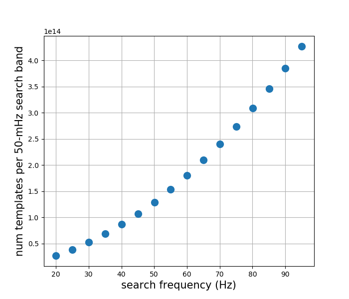
Figure 1: Number of searched templates in 50 mHz band as a function of frequency. The sky resolution increases with frequency causing the variation in the number of templates. $N_{f}\times N_{\dot{f}}\sim 1.3\times 10^{9}$, where $N_{f}$ and $N_{\dot{f}}$ are the number of $f$ and $\dot{f}$ templates searched in 50 mHz bands. The total number of templates searched between 20 and 100 Hz is $3\times 10^{17}$.

Parameter	Value
$T_{\textrm{\mbox{\tiny{coh}}}}$	210 hr
$T_{\textrm{\mbox{\tiny{ref}}}}$	1132729647.5 GPS s
${N_{\mathrm{seg}}}$	12
$\delta f$	$8.3\times 10^{-7}$ Hz
$\delta{\dot{f_{c}}}$	$1.3\times 10^{-11}$ Hz/s
$\gamma$	100
$m_{\text{sky}}$	$1\!\times\!10^{-3}$

Table 1: Search parameters rounded to the first decimal figure. $T_{\textrm{\mbox{\tiny{ref}}}}$ is the reference time that defines the frequency and frequency derivative values.

This search leverages the computing power of the Einstein@Home project, which is built upon the BOINC (Berkeley Open Infrastructure for Network Computing) architecture Boinc1 ; Boinc2 ; Boinc3 : a system that exploits the idle time on volunteer computers to solve scientific problems that require large amounts of computer power. The search is split into work-units (WUs) sized to keep the average Einstein@Home volunteer computer busy for about 8 CPU-hours. Each WU performs $1.5\times 10^{11}$  semi-coherent searches, one for each of the templates in $50$ mHz band, the entire spindown range and 118 points in the sky. Out of the semicoherent detection statistic values computed for the $1.5\times 10^{11}$  templates, it returns to the Einstein@Home server only the highest 10000 values. A total of 1.9 million WUs are necessary to cover the entire parameter space. The total number of templates searched is $3\times 10^{17}$.

III.1 The ranking statistic

Two detection statistics are used in the search: ${\hat{\beta}}_{{{\mathrm{{S}}}/{\mathrm{{G}}{\mathrm{{L}}}{\mathrm{t{L}}}}}}$ and $2\overline{\mathcal{F}}$. ${\hat{\beta}}_{{{\mathrm{{S}}}/{\mathrm{{G}}{\mathrm{{L}}}{\mathrm{t{L}}}}}}$ is the ranking statistic which defines the top-candidate-list; it is a line- and transient-robust statistic that tests the signal hypothesis against a noise model which, in addition to Gaussian noise, also includes single-detector continuous or transient spectral lines. Since the distribution of ${\hat{\beta}}_{{{\mathrm{{S}}}/{\mathrm{{G}}{\mathrm{{L}}}{\mathrm{t{L}}}}}}$ is not known in closed form even in Gaussian noise, when assessing the significance of a candidate against Gaussian noise, we use the average $2\mathcal{F}$ statistic over the segments, $2\overline{\mathcal{F}}$ cutler , see Eq. 1. This is in essence, at every template point, the log-likelihood of having a signal with the shape given by the template versus having Gaussian noise.

Built from the multi- and single-detector $\widehat{\mathcal{F}}$-statistics, ${\hat{\beta}}_{{{\mathrm{{S}}}/{\mathrm{{G}}{\mathrm{{L}}}{\mathrm{t{L}}}}}}$ is the log₁₀ of $\hat{B}_{{{\mathrm{{S}}}/{\mathrm{{G}}{\mathrm{{L}}}{\mathrm{t{L}}}}}}$, the full definition of which is given by Eq. (23) of Keitel:2016 . This statistic depends on a few tuning parameters that we describe in the remainder of the paragraph for the reader interested in the technical details: A transition-scale parameter $\widehat{\mathcal{F}}_{*}^{(0)}$ is used to tune the behaviour of the ${\hat{\beta}}_{{{\mathrm{{S}}}/{\mathrm{{G}}{\mathrm{{L}}}{\mathrm{t{L}}}}}}$ statistic to match the performance of the standard average $2\overline{\mathcal{F}}$ statistic in Gaussian noise while still statistically outperforming it in the presence of continuous or transient single-detector spectral disturbances. Based on injection studies of fake signals in Gaussian-noise data, we set an average $2\overline{\mathcal{F}}$ transition scale of $\widehat{\mathcal{F}}_{*}^{(0)}=65.826$. According to Eq. 67 of Keitel:2013 , with ${N_{\mathrm{seg}}}=12$ this $2\overline{\mathcal{F}}$ value corresponds to a Gaussian false-alarm probability of $10^{-9}$. Furthermore, we assume equal-odds priors between the various noise hypotheses (“L” for line, “G” for Gaussian, “tL” for transient-line).

III.2 Identification of undisturbed bands

Even after the removal of disturbed data caused by spectral artefacts of known origin, the statistical properties of the results are not uniform across the search band. In what follows we concentrate on the subset of the signal-frequency bands having reasonably uniform statistical properties, or containing features that are not immediately identifiable as detector artefacts. This comprises the large majority of the search parameter space.

Our classification of “clean” vs. “disturbed” bands has no pretence of being strictly rigorous, because strict rigour here is neither useful nor practical. The classification serves the practical purpose of discarding from the analysis regions in parameter space with evident disturbances and must not dismiss detectable real signals. The classification is carried out in two steps: an automated identification of undisturbed bands and a visual inspection of the remaining bands.

An automatic procedure, described in Section IIF of S6EHCasA , identifies as undisturbed the 50-mHz bands whose maximum density of outliers in the $f-\dot{f}$ plane and average $2\overline{\mathcal{F}}$ are well within the bulk distribution of the values for these quantities in the neighbouring frequency bands. This procedure identifies $1233$ of the $1600$ 50-mHz bands as undisturbed. The remaining $367$ bands are marked as potentially disturbed, and in need of visual inspection.

A scientist performs the visual inspection by looking at various distributions of the ${\hat{\beta}}_{{{\mathrm{{S}}}/{\mathrm{{G}}{\mathrm{{L}}}{\mathrm{t{L}}}}}}$ statistic over the entire sky and spindown parameter space in the $367$ potentially disturbed 50-mHz bands. She ranks each band with an integer score 0,1,2 ranging from “undisturbed” (0) to “disturbed” (2) . A band is considered “undisturbed” if the distribution of detection statistic values does not show a visible trend affecting a large portion of the $f-\dot{f}$ plane. A band is considered “mildly disturbed” if there are outliers in the band that are localised in a small region of the $f-\dot{f}$ plane. A band is considered “disturbed” if there are outliers that are not well localised in the $f-\dot{f}$ plane.

Fig. 2 shows the ${\hat{\beta}}_{{{\mathrm{{S}}}/{\mathrm{{G}}{\mathrm{{L}}}{\mathrm{t{L}}}}}}$ for each type of band. Fig. 3 shows the ${\hat{\beta}}_{{{\mathrm{{S}}}/{\mathrm{{G}}{\mathrm{{L}}}{\mathrm{t{L}}}}}}$ for a band that harbours a fake signal injected in the data to verify the detection pipelines. In the latter case, the detection statistic is elevated in a small region around the signal parameters.

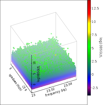
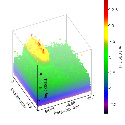
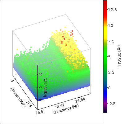
Figure 2: On the vertical axis and color-coded is the ${\hat{\beta}}_{{{\mathrm{{S}}}/{\mathrm{{G}}{\mathrm{{L}}}{\mathrm{t{L}}}}}}$ in three 50-mHz bands. The top band was marked as “undisturbed”. The middle band is an example of a “mildly disturbed band”. The bottom band is an example of a “disturbed band”.

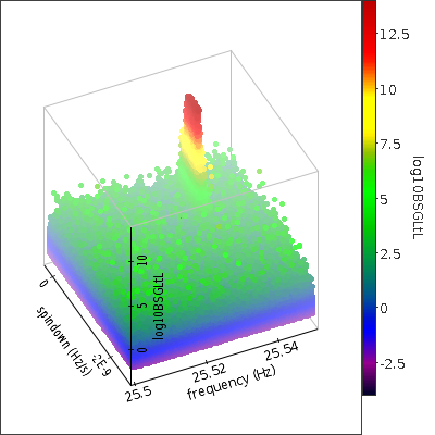
Figure 3: This is an example of an “undisturbed band” but containing a fake signal. On the z-axis and color-coded is the ${\hat{\beta}}_{{{\mathrm{{S}}}/{\mathrm{{G}}{\mathrm{{L}}}{\mathrm{t{L}}}}}}$.

Based on this visual inspection, 1% of the bands between 20 and 100 Hz are marked as “disturbed” and excluded from the current analysis. A further 6% of the bands are marked as “mildly disturbed”. These bands contain features that can not be classified as detector disturbances without further study, therefore these are included in the analysis.

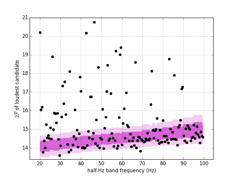
Figure 4: Highest $2\overline{\mathcal{F}}$ value (also referred to as the $2\overline{\mathcal{F}}$ of the loudest candidate) in every half-Hz band as a function of band frequency. Since the number of templates increases with frequency, so does the highest $2\overline{\mathcal{F}}$. The highest expected $2\overline{\mathcal{F}}\pm 1\sigma(2\sigma)$ over $N_{\text{trials}}$ independent trials is indicated by the darker (faded) band. Two half-mHz bands have $2\overline{\mathcal{F}}$ values greater than the axes boundaries. The half-Hz bands beginning at 33.05 Hz and 35.55 Hz have loudest $2\overline{\mathcal{F}}$ values of 159 and 500 respectively, due to features in the 33.3 Hz and 35.75 Hz 50-mHz bands which were marked “mildly disturbed” in the visual inspection.

Fig. 4 shows the highest values of the detection statistic in half-Hz signal-frequency bands compared to the expectations. The set of candidates from which the highest detection statistic values are picked, does not include the 50-mHz signal-frequency bands that stem entirely from fake data, from the cleaning procedure, or that were marked as disturbed. Two 50-mHz bands that contained a hardware injection Biwer:2016oyg were also excluded, as the high amplitude of the injected signal caused it to dominate the list of candidates recovered in those bands. In this paper we refer to the candidates with the highest value of the detection statistic as the loudest candidates.

The highest expected value from Gaussian noise over $N_{\text{trials}}$ independent trials of $2\overline{\mathcal{F}}$ is determined by numerical integration of the probability density function given, for example, by Eq. 7 of GalacticCenterSearch . Fitting to the distribution of the highest $2\overline{\mathcal{F}}$ values suggests that $N_{\text{trials}}\simeq\,N_{\text{templ}}$, with $N_{\text{templ}}$ being the number of templates searched.

The p-value for the highest $2\overline{\mathcal{F}}$ measured in any half-Hz band searched with $N_{\text{trials}}$ independent trials is obtained by integrating the expected noise distribution ($\chi^{2}_{4{N_{\mathrm{seg}}}}$ given in Section III) between the observed value and infinity, as done in Eq. 6 of GalacticCenterSearch . The distribution of these p-values is shown in Fig. 5 and it is not consistent with what we expect from Gaussian noise across the measured range. Therefore, we can not exclude the presence of a signal in this data based on this distribution alone, as was done in S6EH .

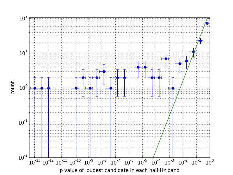
Figure 5: Distribution of p-values, with binomial uncertainties, for the highest detection statistic values measured in half-Hz bands (circles) and expected from pure Gaussian noise (line). We note that the measured p-values for the highest $2\overline{\mathcal{F}}$ in the 33.05 Hz and 35.55 Hz bands are not shown because they are outside of the x-axis boundaries.

IV Hierarchical follow Up

Since the significance of candidates is not consistent with what we expect from Gaussian noise only, we must investigate “significant” candidates to determine if they are produced by a signal or by a detector disturbance. This is done using a hierarchical approach similar to what was used for the hierarchical follow-up of sub-threshold candidates from the Einstein@Home S6 all-sky search S6EHFU .

At each stage of the hierarchical follow-up a semi-coherent search is performed, the top ranking candidates are marked and then searched in the next stage. If the data harbours a real signal, the significance of the recovered candidate will increase with respect to the significance that it had in the previous stage. On the other hand, if the candidate is not produced by a continuous-wave signal, the significance is not expected to increase consistently over the successive stages.

The hierarchical approach used in this search consists of four stages. This is the smallest number of stages within which we could achieve a fully-coherent search, given the available computing resources. Directly performing a fully-coherent follow-up of all significant candidates from the all-sky search would have been computationally unfeasible.

	$T_{\mathrm{coh}}$	${N_{\mathrm{seg}}}$	$\delta f$	$\delta{\dot{f_{c}}}$	$\gamma$	$m_{\text{sky}}$
	hr		Hz	Hz/s
Stage 0	210	12	$8.3\!\times\!10^{-7}$	$1.3\!\times\!10^{-11}$	100	$1\!\times\!10^{-3}$
Stage 1	500	5	$6.7\!\times\!10^{-7}$	$2.9\!\times\!10^{-12}$	80	$8\!\times\!10^{-6}$
Stage 2	1260	2	$1.9\!\times\!10^{-7}$	$9.3\!\times\!10^{-13}$	30	$1\!\times\!10^{-6}$
Stage 3	2512	1	$6.7\!\times\!10^{-8}$	$9.3\!\times\!10^{-14}$	1	$4\!\times\!10^{-7}$

Table 2: Search parameters for each stage. The follow-up stages are stages 1, 2 and 3. Also shown are the parameters for stage-0, taken from Table 1.

IV.1 Stage 0

We bundle together candidates from the all-sky search that can be ascribed to the same root cause. This clustering step is a standard step in a multi-stage approach S6EHFU : Both a loud signal and a loud disturbance produce high values of the detection statistic at a number of different template grid points, and it is a waste of compute cycles to follow up each of these independently.

We apply a clustering procedure that associates together multiple candidates close to each other in parameter space, and assigns them the parameters of the loudest among them, the seed. We use a new procedure with respect to S6EHFU that adapts the cluster size to the data and checks for consistency of the cluster volume with what is expected from a signal AvAC . A candidate must have a ${\hat{\beta}}_{{{\mathrm{{S}}}/{\mathrm{{G}}{\mathrm{{L}}}{\mathrm{t{L}}}}}}>5.5$ to be a cluster seed. This threshold is chosen such that only a handful of candidates per 50-mHz would be selected if the data were consistent with Gaussian noise. In this search, there are 15 million candidates with ${\hat{\beta}}_{{{\mathrm{{S}}}/{\mathrm{{G}}{\mathrm{{L}}}{\mathrm{t{L}}}}}}>5.5$. A lower threshold of ${\hat{\beta}}_{{{\mathrm{{S}}}/{\mathrm{{G}}{\mathrm{{L}}}{\mathrm{t{L}}}}}}>4.0$ is applied to candidates that can be included in a cluster. If a cluster has at least two occupants (including the seed), the seed is marked for follow-up. In total, $35963$ seeds are marked for follow up. The ${\hat{\beta}}_{{{\mathrm{{S}}}/{\mathrm{{G}}{\mathrm{{L}}}{\mathrm{t{L}}}}}}$ values of these candidates are shown in Fig. 6 as well as their distribution in frequency.

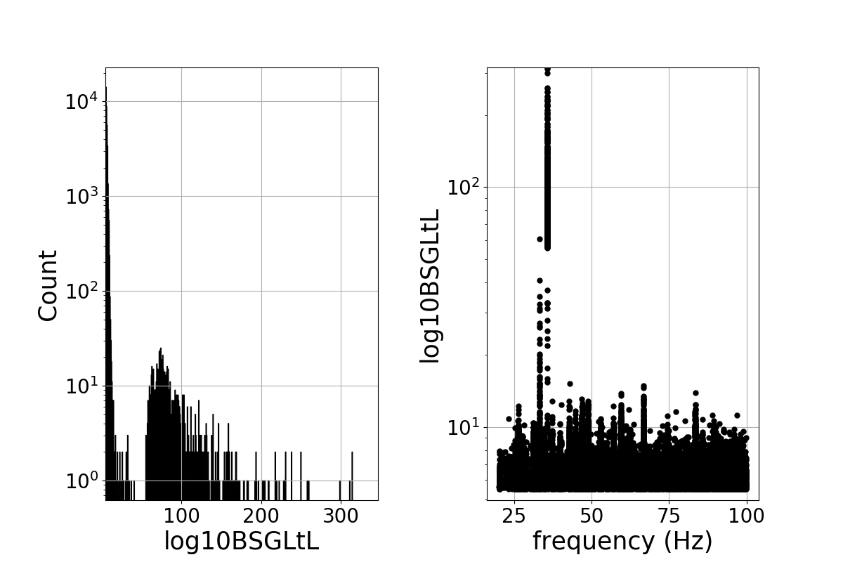
Figure 6: Candidates that are followed-up in stage 1 : the distribution of their detection statistic values ${\hat{\beta}}_{{{\mathrm{{S}}}/{\mathrm{{G}}{\mathrm{{L}}}{\mathrm{t{L}}}}}}$ (left plot) and their distribution as a function of frequency (right plot).

Monte Carlo studies, using simulated signals added into the data, are conducted to determine how far from the signal parameters a signal candidate is recovered. These signals are simulated at a fixed strain amplitude for which most have ${\hat{\beta}}_{{{\mathrm{{S}}}/{\mathrm{{G}}{\mathrm{{L}}}{\mathrm{t{L}}}}}}\gtrapprox 10.0$. We find that $1282$ of $1294$ signal candidates recovered after clustering (99%) are recovered within

$$\begin{cases}\Delta f&=\pm 9.25\times 10^{-5}\,{\textrm{Hz}}\\ \Delta\dot{f}&=\pm 4.25\times 10^{-11}\,{\textrm{Hz/s}}\\ \Delta{\text{sky}}&\simeq 4.5\;{\textrm{sky grid points}}\end{cases}$$ (3)

of the signal parameters. This confidence region defines the parameter space around each candidate which will be searched in the first stage of the hierarchical follow up. For weaker signals the confidence associated with this uncertainty region decreases. For signals close to the threshold used here, namely with ${\hat{\beta}}_{{{\mathrm{{S}}}/{\mathrm{{G}}{\mathrm{{L}}}{\mathrm{t{L}}}}}}$ between 5.5 and 10, the detection confidence only drops by a few percent (see bottom panel of Fig.7 and last row of Table II in AvAC ).

IV.2 Stage 1

In this stage we search a volume of parameter space (Eqs. 3) around each cluster seed. We fix the run time per candidate to be 4 hours on an average CPU of the ATLAS computing cluster ATLAS . This yields an optimal search set-up having a coherent baseline of 500 hours, with 5 segments and the grid spacings shown in Table 2. We use the same ranking statistic as the original search, ${\hat{\beta}}_{{{\mathrm{{S}}}/{\mathrm{{G}}{\mathrm{{L}}}{\mathrm{t{L}}}}}}$, with tunings updated for ${N_{\mathrm{seg}}}=5$.

For the population of simulated signals that passed the previous stage, stage 0, $1268$ of $1282$ (99%) are recovered within the uncertainty region

$$\begin{cases}\Delta f&=\pm 1.76\times 10^{-5}\,{\textrm{Hz}}\\ \Delta\dot{f}&=\pm 9.6\times 10^{-12}\,{\textrm{Hz/s}}\\ \Delta{\text{sky}}&\simeq 0.23~{}\Delta{\text{sky}}^{\text{ Stage-0}}.\end{cases}$$ (4)

From each of the $35963$ follow-up searches we record the most significant candidate in ${\hat{\beta}}_{{{\mathrm{{S}}}/{\mathrm{{G}}{\mathrm{{L}}}{\mathrm{t{L}}}}}}$. The distribution of these is shown in Fig. 7. A threshold at ${\hat{\beta}}_{{{\mathrm{{S}}}/{\mathrm{{G}}{\mathrm{{L}}}{\mathrm{t{L}}}}}}$ = 6.0, derived from Monte Carlo studies, is applied to select the candidates to consider in the next stage. There are $14456$ candidates above this threshold.

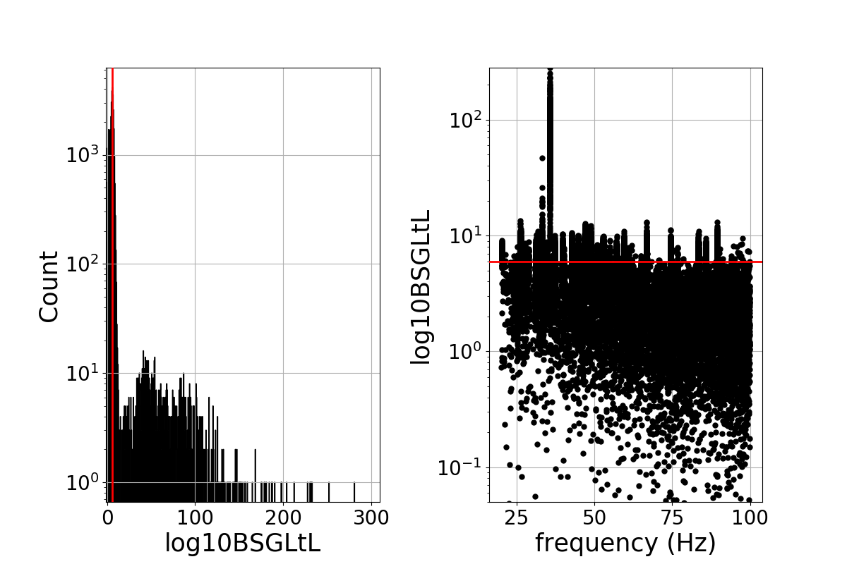
Figure 7: Detection statistic of the loudest candidate from each stage-1 search: the distribution of their detection statistic values ${\hat{\beta}}_{{{\mathrm{{S}}}/{\mathrm{{G}}{\mathrm{{L}}}{\mathrm{t{L}}}}}}$ (left plot) and their distribution as a function of frequency (right plot). 411 candidates have ${\hat{\beta}}_{{{\mathrm{{S}}}/{\mathrm{{G}}{\mathrm{{L}}}{\mathrm{t{L}}}}}}$ values lower than the axes boundaries on the right plot. The red line marks ${\hat{\beta}}_{{{\mathrm{{S}}}/{\mathrm{{G}}{\mathrm{{L}}}{\mathrm{t{L}}}}}}$ = 6.0 which is the threshold at and above which candidates are passed on to stage-2.

IV.3 Stage 2

In this stage we search a volume of parameter space (Eqs. 4) around each candidate from stage-1. We fix the run time per candidate to be 4 hours on an average CPU of the ATLAS computing cluster ATLAS . This yields an optimal search set-up having a coherent baseline of 1260 hours, with 2 segments and the grid spacings shown in Table 2. We use a different ranking statistic from the original search, because with 2 segments the transient line veto is not useful. Instead we use the ranking statistic ${\hat{\beta}}_{{{\mathrm{{S}}}/{\mathrm{{G}}{\mathrm{{L}}}}}}:=\log_{10}\hat{B}_{{{\mathrm{{S}}}/{\mathrm{{G}}{\mathrm{{L}}}}}}$, introduced in Keitel:2013 and previously used in S6EH , with tunings updated for ${N_{\mathrm{seg}}}=2$.

For the population of signals that passed the previous stage, $1265$ of $1268$ ($>99\%$) are recovered within the uncertainty region

$$\begin{cases}\Delta f&=\pm 8.65\times 10^{-6}\,{\textrm{Hz}}\\ \Delta\dot{f}&=\pm 7.8\times 10^{-12}\,{\textrm{Hz/s}}\\ \Delta{\text{sky}}&\simeq 0.81~{}\Delta{\text{sky}}^{\text{ Stage-1}}.\end{cases}$$ (5)

From each of the follow-up searches we record the most significant candidate in ${\hat{\beta}}_{{{\mathrm{{S}}}/{\mathrm{{G}}{\mathrm{{L}}}}}}$. The distribution of these is shown in Fig. 8. A threshold at ${\hat{\beta}}_{{{\mathrm{{S}}}/{\mathrm{{G}}{\mathrm{{L}}}}}}$ = 6.0 is applied to determine what candidates to consider in the next stage. There are $8486$ candidates above threshold.

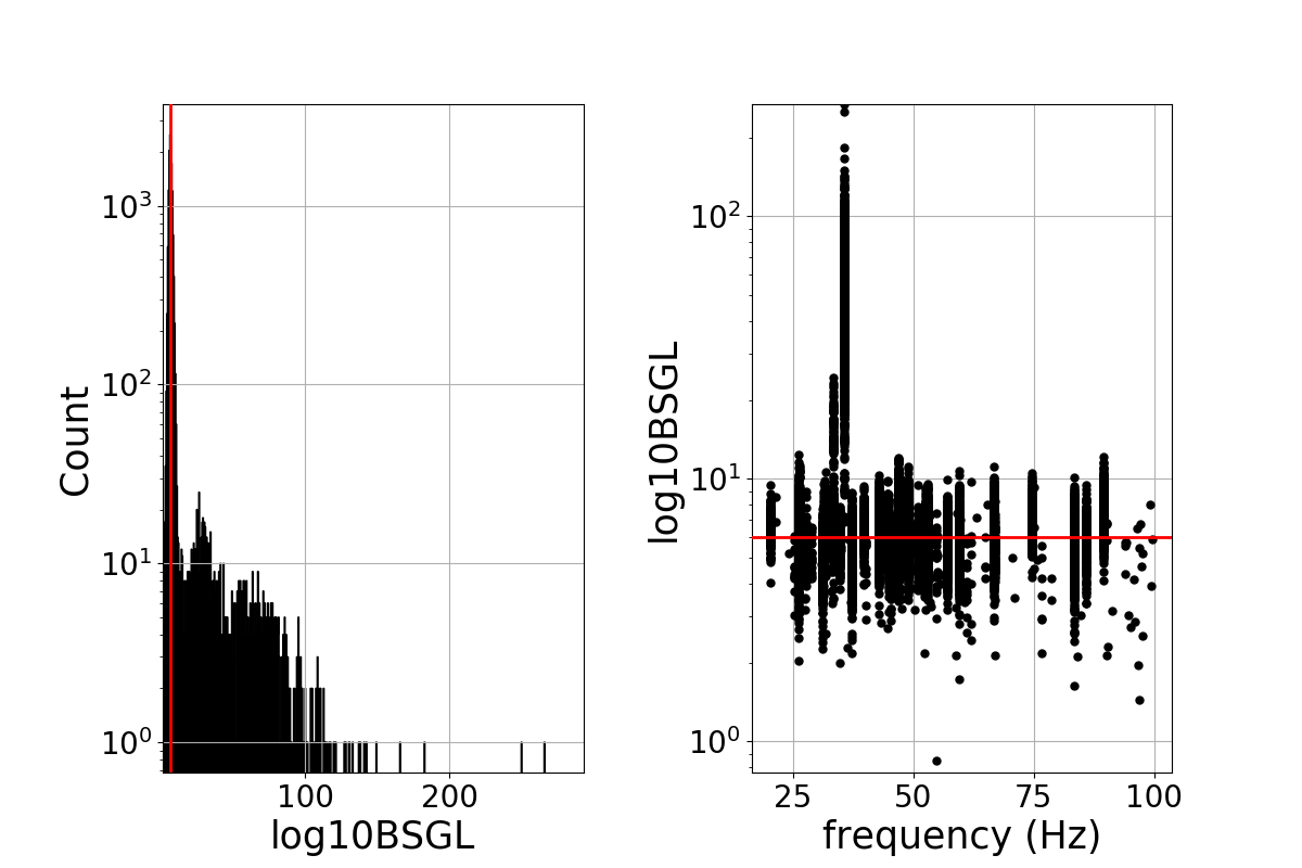
Figure 8: Detection statistic of the loudest candidate from each stage-2 search: the distribution of their detection statistic values ${\hat{\beta}}_{{{\mathrm{{S}}}/{\mathrm{{G}}{\mathrm{{L}}}}}}$ (left plot) and their distribution as a function of frequency (right plot). The red line marks ${\hat{\beta}}_{{{\mathrm{{S}}}/{\mathrm{{G}}{\mathrm{{L}}}}}}$ = 6.0 which is the threshold at and above which candidates are passed on to stage-3.

IV.4 Stage 3

In this stage we search a volume of parameter space (Eqs. 5) around each candidate. We perform a fully coherent search, with a coherent baseline of 2512 hours. The grid spacings are shown in Table 2. We use the same ranking statistic as the previous stage, ${\hat{\beta}}_{{{\mathrm{{S}}}/{\mathrm{{G}}{\mathrm{{L}}}}}}$, with tunings updated for ${N_{\mathrm{seg}}}=1$.

For the population of signals that passed the previous stage, $1265$ of $1265$ ($>99\%$) are recovered within the uncertainty region

$$\begin{cases}\Delta f&=\pm 7.5\times 10^{-6}\,{\textrm{Hz}}\\ \Delta\dot{f}&=\pm 7\times 10^{-12}\,{\textrm{Hz/s}}\\ \Delta{\text{sky}}&\simeq 0.99~{}\Delta{\text{sky}}^{\text{ Stage-2}}.\end{cases}$$ (6)

This uncertainty region assumes candidates are within the uncertainty regions shown in Eqs. 3, 4 and 5 for each of the corresponding follow-up stages. It is possible that a strong candidate which is outside these uncertainty regions would be significant enough to pass through all follow-up stages. In this case the uncertainty on the signal parameters would be larger than the uncertainty region defined in Eq. 6.

From each of the follow-up searches we record the most significant candidate in ${\hat{\beta}}_{{{\mathrm{{S}}}/{\mathrm{{G}}{\mathrm{{L}}}}}}$. The distribution of these is shown in Fig. 9. A threshold at ${\hat{\beta}}_{{{\mathrm{{S}}}/{\mathrm{{G}}{\mathrm{{L}}}}}}$ = 6.0 is applied to determine what candidates require further study. There are $6349$ candidates above threshold. Many candidates appear to be from the same feature at a specific frequency. There are 57 distinct narrow frequency regions at which these $6349$ candidates have been recovered.

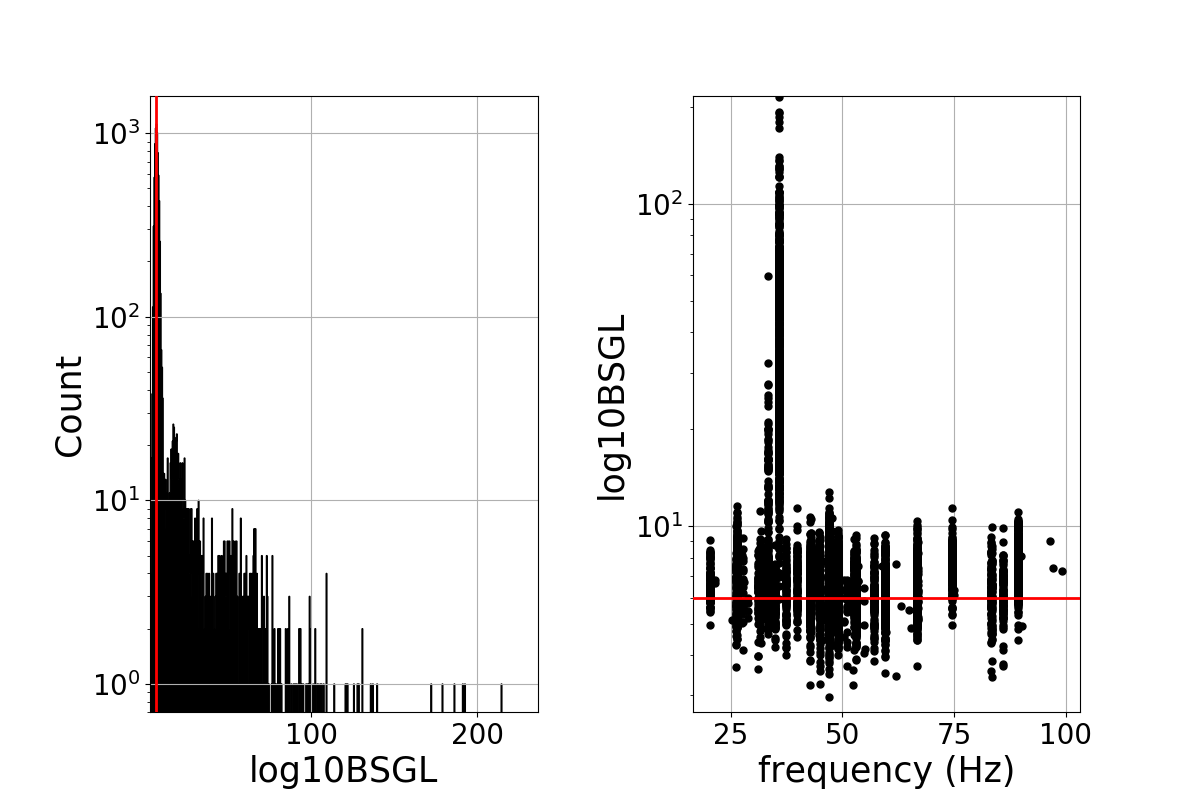
Figure 9: Detection statistic of the loudest candidate from each stage-3 search: the distribution of their detection statistic values ${\hat{\beta}}_{{{\mathrm{{S}}}/{\mathrm{{G}}{\mathrm{{L}}}}}}$ (left plot) and their distribution as a function of frequency (right plot). The red line marks ${\hat{\beta}}_{{{\mathrm{{S}}}/{\mathrm{{G}}{\mathrm{{L}}}}}}$ = 6.0 which is the threshold below which candidates are discarded.

IV.5 Doppler Modulation off veto

We employ a newly developed Doppler modulation off (DM-off) veto DM-off to determine if the surviving candidates are of terrestrial origin. When searching for CW signals, the frequency of the signal template at any point in time is demodulated for the Doppler effect from the motion of the detectors around the earth and around the sun. If this de-modulation is disabled, a candidate of astrophysical origin would not be recovered with the same significance. In contrast, a candidate of terrestrial origin could potentially become more significant. This is the basis of the DM-off veto.

For each candidate, the search range of the DM-off searches includes all detector frequencies that could have contributed to the original candidate, accounting for $\dot{f}$ and Doppler corrections. The $\dot{f}$ range includes the original all-sky search range, and extends into large positive values of $\dot{f}$ to allow for a wider range of detector artefact behaviour.

For a candidate to pass the DM-off veto it must be that its $2\mathcal{F}_{\textrm{DM-off}}\leq 2\mathcal{F}^{\textrm{thr}}_{\textrm{DM-off}}$. The $2\mathcal{F}^{\textrm{thr}}_{\textrm{DM-off}}$ is picked to be safe, i.e. to not veto any signal candidate with $2\mathcal{F}_{\textrm{DM-on}}$ in the range of the candidates under consideration. In particular we find that for candidates with $2\mathcal{F}_{\textrm{DM-on}}<500$, after the third follow-up, $2\mathcal{F}^{\textrm{thr}}_{\textrm{DM-off}}=62$. The threshold increases for candidates with $2\mathcal{F}_{\textrm{DM-on}}>500$, scaling linearly with the candidates $2\mathcal{F}_{\textrm{DM-on}}$ (see Figure 4 of DM-off ).

As described in DM-off , the DM-off search is first run using data from both detectors and a search grid which is ten times coarser in $f$ and $\dot{f}$ than the stage-3 search. $653$ of the $6349$ candidates pass the $2\mathcal{F}^{\textrm{thr}}_{\textrm{DM-off}}$ threshold. These surviving candidates undergo another similar search, except that the search is performed separately on the data from each of the LIGO detectors. $101$ candidates survive, and undergo a final DM-off search stage. This search uses the fine grid parameters of the stage-3 search (Table 2), covers the parameter space which resulted in the largest $2\mathcal{F}_{\textrm{DM-off}}$ from the previous DM-off steps, and is performed using both detectors jointly and each detector separately. For a candidate to survive this stage it has to pass all three stage-3 searches.

Four candidates survive the full DM-off veto. The parameters of the candidates, after the third follow-up, are given in Table 3. The $2\mathcal{F}_{\textrm{DM-off}}$ values are also given in this table.

ID	$f$ [Hz]	$\alpha$ [rad]	$\delta$ [rad]	${\dot{f}}$ [Hz/s]	$2\overline{\mathcal{F}}$	$2\overline{\mathcal{F}}_{\text{H1}}$	$2\overline{\mathcal{F}}_{\text{L1}}$	$2\mathcal{F}_{\textrm{DM-off}}$
$1$	$58.970435900$	$1.87245$	$-0.51971$	$-1.081102\times 10^{-9}$	$81.4$	$48.5$	$33.4$	$55$
$2$	$62.081409292$	$4.98020$	$0.58542$	$-2.326246\times 10^{-9}$	$81.9$	$45.5$	$39.0$	$52$
$3$	$97.197674733$	$5.88374$	$-0.76773$	$2.28614\times 10^{-10}$	$86.5$	$55.0$	$31.8$	$58$
$4$	$99.220728369$	$2.842702$	$-0.469603$	$-2.498113\times 10^{-9}$	$80.2$	$41.4$	$45.8$	$55$

Table 3: Stage-3 follow-up results for each of the 4 candidates that survive the DM-off veto. For illustration purposes in the 7th and 8th column we show the values of the average single-detector detection statistics. Typically, for signals, the single-detector values do not exceed the multi-detector $2\overline{\mathcal{F}}$.

IV.6 Follow-up in LIGO O2 data

If the signal candidates surviving the O1 search are standard continuous-wave signals, i.e. continuous wave signals arising from sources that radiate steadily over many years, they should be present in data from the Advanced LIGO’s second observing run (O2) with the same parameters. We perform a follow-up search using three months of O2 data, collected from November 30 2016 to February 28 2017.

The candidate parameters in Table 3 are translated to the O2 midtime, which is the reference time of the new search. The parameter space covered by the search is determined by the uncertainty on the candidate parameters in Eq. 5. The frequency region is widened to account for the spindown uncertainty. The O2 follow-up covers a frequency range of $\pm 5.15\times 10^{-4}$ Hz around the candidates.

The search parameters of the O2 follow-up are given in Table 4. The expected loudest $2\overline{\mathcal{F}}$ per follow-up search due to Gaussian noise alone, is $52\pm 3$, assuming independent search templates.

If a candidate in Table 3 were due to a signal, the loudest $2\overline{\mathcal{F}}$ expected after the follow-up would be the value given in the second column of Table 5. This expected value is obtained by scaling the $2\overline{\mathcal{F}}$ in Table 3 according to the different duration and the different noise levels between the data set used for the third follow-up and the O2 data set. The expected $2\overline{\mathcal{F}}$ also folds-in a conservative factor of 0.9 due to a different mismatch of the O2 template grid with respect to the template grid used for the third follow-up. Thus the expected $2\overline{\mathcal{F}}$ in Table 5 is a conservative estimate for the minimum $2\overline{\mathcal{F}}$ that we would expect from a signal candidate.

The loudest $2\overline{\mathcal{F}}$ after the follow-up in O2 data is also given in Table 5. The loudest $2\overline{\mathcal{F}}$ recovered for each candidate are $\approx 2\sigma$ below the expected $2\overline{\mathcal{F}}$ for a signal candidate. The recovered $2\overline{\mathcal{F}}$ are consistent with what is expected from Gaussian data. We conclude that it is unlikely that any of the candidates in Table III arises from a long-lived astronomical source of continuous gravitational waves.

Parameter	Value
$T_{\textrm{\mbox{\tiny{coh}}}}$	2160 hrs
$T_{\textrm{\mbox{\tiny{ref}}}}$	1168447494.5 GPS sec
${N_{\mathrm{seg}}}$	1
$\delta f$	$9.0\times 10^{-8}$ Hz
$\delta{\dot{f_{c}}}$	$1.1\times 10^{-13}$ Hz/s
$\gamma$	1
$m_{\text{sky}}$	$4\!\times\!10^{-7}$

Table 4: Search parameters, rounded to the first decimal place, for the follow-up of surviving LIGO O1 candidates in LIGO O2 data. $T_{\textrm{\mbox{\tiny{ref}}}}$ is the reference time that defines the frequency and frequency derivative values.

Candidate	Expected $2\overline{\mathcal{F}}\pm 1\sigma$	Loudest $2\overline{\mathcal{F}}$ recovered
1	$85\pm 18$	$44$
2	$90\pm 19$	$52$
3	$84\pm 18$	$49$
4	$77\pm 17$	$47$

Table 5: Highest $2\overline{\mathcal{F}}$ expected after the follow-up in O2 data, if the candidates were due to a signal, compared with the highest $2\overline{\mathcal{F}}$ recovered from the follow-up. The $2\overline{\mathcal{F}}$ expected in Gaussian noise data is $52\pm 3$.

V Results

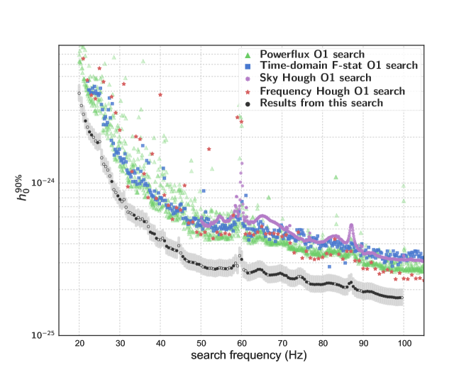
Figure 10: 90% confidence upper limits on the gravitational wave amplitude of continuous gravitational wave signals with frequency in 0.5 Hz bands and with spindown values within the searched range. The lowest set of points (black circles) are the results of this search. The empty circles denote half-Hz bands where the upper limit value does not hold for all frequencies in that interval. A list of the excluded frequencies is given in the Appendix. The lighter grey region around the upper limit points shows the 11% relative difference bracket between upper limits inferred with the procedure described in Section V and upper limits that would have been derived (at great computational expense) with direct measurements in all half-Hz bands. We estimate that less than $\sim 0.5\%$ of the upper limit points would fall outside of this bracket if they were derived with the direct-measurement method in Gaussian noise. For comparison we also plot the most recent upper limits results in this frequency range from O1 data obtained with various search pipelines O1ASMulti . We note that these searches cover a broader frequency and spindown range than the search presented here. All upper limits presented here are population-averaged limits over the full sky and source polarisation.

The search did not reveal any continuous gravitational wave signal in the parameter volume that was searched. We hence set frequentist 90% confidence upper limits on the maximum gravitational wave amplitude consistent with this null result in $0.5$ Hz bands, $h_{0}^{90\%}(f)$. Specifically, $h_{0}^{90\%}(f)$ is the GW amplitude such that 90% of a population of signals with parameter values in our search range would have been detected by our search. We determined the upper limits in bands that were marked as undisturbed in Section III.2. These upper limits may not hold for frequency bands that were marked as mildly disturbed, which we now consider disturbed as they were excluded by the analysis. These bands, as well as bands which were excluded from further analysis, are identified in Appendix A.3.

Since an actual full scale fake-signal injection-and-recovery Monte Carlo for the entire set of follow-ups in every $0.5$ Hz band is prohibitive, in the same spirit as S6EHFU ; S6EHCasA ; S5GC1HF , we perform such a study in a limited set of trial bands. We choose 20 half-Hz bands to measure the upper limits. If these half-Hz bands include 50-mHz bands which were not marked undisturbed, no upper limit injections are made in those 50-mHz bands.

The amplitudes of the fake signals bracket the 90% confidence region typically between 70% and 100%. The $h_{0}$ versus confidence data is fit in this region with a sigmoid of the form

$$C(h_{0})={1\over{1+\exp({{{\textrm{a}}-h_{0}}\over{\textrm{b}}})}}$$ (7)

and the $h_{0}^{90\%}$ value is read-off of this curve. The fitting procedure yields the best-fit a and b values and the covariance matrix. Given the binomial confidence values uncertainties, using the covariance matrix we estimate the $h_{0}^{90\%}$ uncertainty.

For each of these frequency bands we determine the sensitivity depth ${{\mathcal{D}}}^{90\%}$ GalacticCenterMethod of the search corresponding to $h_{0}^{90\%}(f)$:

$${{\mathcal{D}}}^{90\%}:={\sqrt{S_{h}(f)}\over{h_{0}^{90\%}(f)}}~{}~{}[{1/\sqrt{\text{Hz}}}],$$ (8)

where $\sqrt{S_{h}(f)}$ is the noise level of the data as a function of frequency.

As representative of the sensitivity depth of this hierarchical search, we take the average of the measured depths at different frequencies: $48.7~{}[{1/\sqrt{\text{Hz}}}]$. We then determine the 90% upper limits by substituting this value in Eq. 8 for ${{\mathcal{D}}}^{90\%}$.

The upper limit that we get with this procedure, in general yields a different number compared to the upper limit directly measured as done in the twenty test bands. An $11\%$ relative error bracket comprises the range of variation observed on the measured sensitivity depths, including the uncertainties on the single measurements. So we take this as a generous estimate of the range of variability of the upper limit values introduced by the estimation procedure. If the data were Gaussian this bracket would yield a $\sim 0.5\%$ probability of a measured upper limit falling outside of this bracket.

Figure 10 shows these upper limits as a function of frequency. They are also presented in tabular form in the Appendix with the uncertainties indicating the range of variability introduced by the estimation procedure. The associated uncertainties amount to $\sim 20\%$ when also including 10% amplitude calibration uncertainty. The most constraining upper limit in the band 98.5-99 Hz, close to the highest frequency, where the detector is most sensitive, is $1.8\times 10^{-25}$. At the lowest end of the frequency range, at 20 Hz, the upper limit rises to $3.9\times 10^{-24}$.

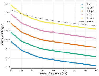
Figure 11: Ellipticity $\epsilon$ of a source at a distance d emitting continuous gravitational waves that would have been detected by this search. The dashed line shows the spin-down ellipticity for the highest magnitude spindown parameter value searched: 2.6 $\times 10^{-9}$ Hz/s. The spin-down ellipticity is the ellipticity necessary for all the lost rotational kinetic energy to be emitted in gravitational waves. If we assume that the observed spin-down is all actual spin-down of the object, then no ellipticities could be possible above the dashed curve. In reality the observed and actual spindown could differ due to radial acceleration of the source. In this case the actual spin-down of the object may even be larger than the apparent one. In this case our search would be sensitive to objects with ellipticities above the dashed line.

In general not all the rotational kinetic energy lost is due to GW emission. Following Ming:2015jla , we define $x$ to be the fraction of the spindown rotational energy emitted in gravitational waves. The star’s ellipticity necessary to sustain such emission is

$$\epsilon(f,x{\dot{f}})=\sqrt{{5c^{5}\over 32\pi^{4}G}{x{|\dot{f}|}\over If^{5}}},$$ (9)

where $c$ is the speed of light, $G$ is the gravitational constant, $f$ is the GW frequency and $I$ the principal moment of inertia of the star. Correspondingly, $x{\dot{f}}$ is the spindown rate that accounts for the emission of GWs and this is why we refer to it as the GW spindown. The gravitational wave amplitude $h_{0}$ at the detector coming from a GW source like that of Eq. 9, at a distance $D$ from Earth is

$$h_{0}(f,x\dot{f},D)={1\over D}\sqrt{{5GI\over 2c^{3}}{x{|\dot{f}|}\over f}}.$$ (10)

Based on this last equation, we can use the GW amplitude upper limits to bound the minimum distance for compact objects emitting continuous gravitational waves under different assumptions on the object’s ellipticity (i.e. gravitational wave spindown). This is shown in Fig. 11. Above 55 Hz we can exclude sources with ellipticities larger than $10^{-5}$ within 100 pc of Earth. Rough estimates are that there should be of order $10^{4}$ neutron stars within this volume.

VI Conclusions

This search concentrates the computing power of Einstein@Home in a relatively small frequency range at low frequencies where all-sky searches are significantly “cheaper” than at higher frequencies. For this reason, the initial search could be set-up with a very long coherent observation time of 210 hours and this yields a record sensitivity depth of 48.7 [1/$\sqrt{\textrm{Hz}}$].

The O1 data set in the low frequency range investigated with this search is significantly more polluted by coherent spectral artefacts than most of the data sets from the Initial-LIGO science runs. Because of this, even a relatively high threshold on the detection statistic of the first search yields tens of thousands of candidates, rather than just $O(100)$. We follow each of them up through a hierarchy of three further stages at the end of which $O(7000)$ survive. After the application of a newly developed Doppler-modulation-off veto, 4 survive. These are finally followed up with a fully coherent search using three months of O2 data, which produces results completely consistent with Gaussian noise and falls short of the predictions under the signal hypothesis. We hence proceed to set upper limits on the intrinsic GW amplitude $h_{0}$. The hierarchical follow-up procedure presented here has also been used to follow-up outliers from other all-sky searches in O1 data with various search pipelines O1ASMulti .

The smallest value of the GW amplitude upper limit is $1.8\times 10^{-25}$ in the band 98.5-99 Hz. Fig. 10 shows the upper limit values as a function of search frequency. Our upper limits are the tightest ever placed for this population of signals, and are a factor 1.5-2 smaller than the most recent upper limits O1ASMulti . We note that O1ASMulti presents results from four different all-sky search pipelines covering a broader frequency and spindown range than the one explored here. The coherent time-baseline for all these pipelines is significantly shorter than the 210 hours used by the very first stage of this search. This limits the sensitivity of those searches but it makes them more robust to deviations in the signal waveform from the target waveform, with respect this search.

Translating the upper limits on the GW amplitude in upper limits on the ellipticity of the GW source, we find that for frequencies above 55 Hz our results exclude isolated compact objects with ellipticities of $10^{-5}{\sqrt{10^{38}\textrm{kg\,m}^{2}/I}}$ (corresponding to GW spindowns between $10^{-14}$ Hz/s and $10^{-13}$ Hz/s) or higher, within 100 pc of Earth.

VII Acknowledgments

The authors gratefully acknowledge the support of the United States National Science Foundation (NSF) for the construction and operation of the LIGO Laboratory and Advanced LIGO as well as the Science and Technology Facilities Council (STFC) of the United Kingdom, the Max-Planck-Society (MPS), and the State of Niedersachsen/Germany for support of the construction of Advanced LIGO and construction and operation of the GEO600 detector. Additional support for Advanced LIGO was provided by the Australian Research Council. The authors gratefully acknowledge the Italian Istituto Nazionale di Fisica Nucleare (INFN), the French Centre National de la Recherche Scientifique (CNRS) and the Foundation for Fundamental Research on Matter supported by the Netherlands Organisation for Scientific Research, for the construction and operation of the Virgo detector and the creation and support of the EGO consortium. The authors also gratefully acknowledge research support from these agencies as well as by the Council of Scientific and Industrial Research of India, Department of Science and Technology, India, Science & Engineering Research Board (SERB), India, Ministry of Human Resource Development, India, the Spanish Ministerio de Economía y Competitividad, the Vicepresidència i Conselleria d’Innovació, Recerca i Turisme and the Conselleria d’Educació i Universitat del Govern de les Illes Balears, the National Science Centre of Poland, the European Commission, the Royal Society, the Scottish Funding Council, the Scottish Universities Physics Alliance, the Hungarian Scientific Research Fund (OTKA), the Lyon Institute of Origins (LIO), the National Research Foundation of Korea, Industry Canada and the Province of Ontario through the Ministry of Economic Development and Innovation, the Natural Science and Engineering Research Council Canada, Canadian Institute for Advanced Research, the Brazilian Ministry of Science, Technology, and Innovation, International Center for Theoretical Physics South American Institute for Fundamental Research (ICTP-SAIFR), Russian Foundation for Basic Research, the Leverhulme Trust, the Research Corporation, Ministry of Science and Technology (MOST), Taiwan and the Kavli Foundation. The authors gratefully acknowledge the support of the NSF, STFC, MPS, INFN, CNRS and the State of Niedersachsen/Germany for provision of computational resources.

The authors also gratefully acknowledge the support of the many thousands of Einstein@Home volunteers, without whom this search would not have been possible.

This document has been assigned LIGO Laboratory document number LIGO-P1700127.

Appendix A Tabular data

A.1 Upper limit values

Table 6: First frequency of each half-Hz signal frequency band in which we set upper limits and upper limit value for that band. The uncertainties correspond to the 11% relative difference bracket discussed in Section V

$f$ (Hz)	$h_{0}^{90\%}\times 10^{25}$		$f$ (Hz)	$h_{0}^{90\%}\times 10^{25}$		$f$ (Hz)	$h_{0}^{90\%}\times 10^{25}$		$f$ (Hz)	$h_{0}^{90\%}\times 10^{25}$
20.00	38.8 $\pm$ 4.9		20.55	32.2 $\pm$ 4.1		21.05	28.2 $\pm$ 3.6		21.55	25.5 $\pm$ 3.3
22.05	23.3 $\pm$ 3.0		22.55	21.6 $\pm$ 2.8		23.05	20.7 $\pm$ 2.6		23.55	19.9 $\pm$ 2.5
24.05	18.9 $\pm$ 2.4		24.55	18.4 $\pm$ 2.3		25.05	18.7 $\pm$ 2.4		25.55	14.6 $\pm$ 1.9
26.05	13.3 $\pm$ 1.7		26.55	12.8 $\pm$ 1.6		27.05	12.2 $\pm$ 1.6		27.55	11.1 $\pm$ 1.4
28.05	10.2 $\pm$ 1.3		28.55	9.0 $\pm$ 1.2		29.05	8.7 $\pm$ 1.1		29.55	8.2 $\pm$ 1.0
30.05	7.8 $\pm$ 1.0		30.55	7.6 $\pm$ 1.0		31.05	7.8 $\pm$ 1.0		31.55	6.9 $\pm$ 0.9
32.05	6.5 $\pm$ 0.8		32.55	6.4 $\pm$ 0.8		33.05	6.3 $\pm$ 0.8		33.55	6.2 $\pm$ 0.8
34.05	5.8 $\pm$ 0.7		34.55	5.9 $\pm$ 0.8		35.05	5.8 $\pm$ 0.7		35.55	5.8 $\pm$ 0.7
36.05	5.6 $\pm$ 0.7		36.55	5.6 $\pm$ 0.7		37.05	5.2 $\pm$ 0.7		37.55	4.8 $\pm$ 0.6
38.05	4.7 $\pm$ 0.6		38.55	4.6 $\pm$ 0.6		39.05	4.3 $\pm$ 0.6		39.55	4.3 $\pm$ 0.5
40.05	4.2 $\pm$ 0.5		40.55	4.3 $\pm$ 0.6		41.05	4.2 $\pm$ 0.5		41.55	3.9 $\pm$ 0.5
42.05	3.8 $\pm$ 0.5		42.55	3.7 $\pm$ 0.5		43.05	3.7 $\pm$ 0.5		43.55	3.6 $\pm$ 0.5
44.05	3.6 $\pm$ 0.5		44.55	3.9 $\pm$ 0.5		45.05	3.5 $\pm$ 0.4		45.55	3.3 $\pm$ 0.4
46.05	3.2 $\pm$ 0.4		46.55	3.1 $\pm$ 0.4		47.05	3.0 $\pm$ 0.4		47.55	3.0 $\pm$ 0.4
48.05	3.0 $\pm$ 0.4		48.55	3.0 $\pm$ 0.4		49.05	2.9 $\pm$ 0.4		49.55	2.9 $\pm$ 0.4
50.05	2.9 $\pm$ 0.4		50.55	2.8 $\pm$ 0.4		51.05	2.8 $\pm$ 0.4		51.55	2.8 $\pm$ 0.4
52.05	2.8 $\pm$ 0.4		52.55	2.8 $\pm$ 0.4		53.05	2.7 $\pm$ 0.3		53.55	2.7 $\pm$ 0.3
54.05	2.7 $\pm$ 0.3		54.55	2.8 $\pm$ 0.4		55.05	2.8 $\pm$ 0.4		55.55	2.7 $\pm$ 0.3
56.05	2.7 $\pm$ 0.3		56.55	2.7 $\pm$ 0.3		57.05	2.8 $\pm$ 0.4		57.55	2.8 $\pm$ 0.4
58.05	2.9 $\pm$ 0.4		58.55	3.0 $\pm$ 0.4		59.05	2.9 $\pm$ 0.4		59.55	3.3 $\pm$ 0.4
60.05	3.2 $\pm$ 0.4		60.55	2.7 $\pm$ 0.3		61.05	2.7 $\pm$ 0.3		61.55	2.6 $\pm$ 0.3
62.05	2.6 $\pm$ 0.3		62.55	2.6 $\pm$ 0.3		63.05	2.6 $\pm$ 0.3		63.55	2.7 $\pm$ 0.3
64.05	2.7 $\pm$ 0.3		64.55	2.7 $\pm$ 0.3		65.05	2.7 $\pm$ 0.3		65.55	2.6 $\pm$ 0.3
66.05	2.5 $\pm$ 0.3		66.55	2.5 $\pm$ 0.3		67.05	2.5 $\pm$ 0.3		67.55	2.5 $\pm$ 0.3
68.05	2.5 $\pm$ 0.3		68.55	2.5 $\pm$ 0.3		69.05	2.5 $\pm$ 0.3		69.55	2.6 $\pm$ 0.3
70.05	2.5 $\pm$ 0.3		70.55	2.5 $\pm$ 0.3		71.05	2.5 $\pm$ 0.3		71.55	2.4 $\pm$ 0.3
72.05	2.4 $\pm$ 0.3		72.55	2.4 $\pm$ 0.3		73.05	2.4 $\pm$ 0.3		73.55	2.4 $\pm$ 0.3
74.05	2.4 $\pm$ 0.3		74.55	2.4 $\pm$ 0.3		75.05	2.4 $\pm$ 0.3		75.55	2.3 $\pm$ 0.3
76.05	2.2 $\pm$ 0.3		76.55	2.2 $\pm$ 0.3		77.05	2.2 $\pm$ 0.3		77.55	2.2 $\pm$ 0.3
78.05	2.2 $\pm$ 0.3		78.55	2.2 $\pm$ 0.3		79.05	2.2 $\pm$ 0.3		79.55	2.2 $\pm$ 0.3
80.05	2.2 $\pm$ 0.3		80.55	2.2 $\pm$ 0.3		81.05	2.2 $\pm$ 0.3		81.55	2.2 $\pm$ 0.3
82.05	2.2 $\pm$ 0.3		82.55	2.2 $\pm$ 0.3		83.05	2.2 $\pm$ 0.3		83.55	2.2 $\pm$ 0.3
84.05	2.1 $\pm$ 0.3		84.55	2.1 $\pm$ 0.3		85.05	2.1 $\pm$ 0.3		85.55	2.1 $\pm$ 0.3
86.05	2.1 $\pm$ 0.3		86.55	2.2 $\pm$ 0.3		87.05	2.2 $\pm$ 0.3		87.55	2.1 $\pm$ 0.3
88.05	2.0 $\pm$ 0.3		88.55	2.0 $\pm$ 0.3		89.05	2.0 $\pm$ 0.3		89.55	2.0 $\pm$ 0.2
90.05	1.9 $\pm$ 0.2		90.55	1.9 $\pm$ 0.2		91.05	2.0 $\pm$ 0.2		91.55	1.9 $\pm$ 0.2
92.05	1.9 $\pm$ 0.2		92.55	1.9 $\pm$ 0.2		93.05	1.9 $\pm$ 0.2		93.55	1.9 $\pm$ 0.2
94.05	1.8 $\pm$ 0.2		94.55	1.8 $\pm$ 0.2		95.05	1.8 $\pm$ 0.2		95.55	1.8 $\pm$ 0.2
96.05	1.8 $\pm$ 0.2		96.55	1.8 $\pm$ 0.2		97.05	1.8 $\pm$ 0.2		97.55	1.8 $\pm$ 0.2
98.05	1.8 $\pm$ 0.2		98.55	1.8 $\pm$ 0.2		99.05	1.8 $\pm$ 0.2		99.55	1.8 $\pm$ 0.2
.

A.2 Cleaned-out frequency bins

Table 7: Instrumental lines identified and “cleaned” before the Einstein@Home runs. The different columns represent: (I) the central frequency of the instrumental line; (II) Low-Frequency-Side (LFS) of the knockout band; (III) High-Frequency-Side (HFS) of the knockout band; (IV) the interferometer in which the instrumental lines were identified.

$f_{\mathrm{L}}$ (Hz)	LFS (Hz)	HFS (Hz)	IFO
19.9995	0.001	0.001	L
20.0	0.001	0.001	H
20.24999	0.001	0.001	H
20.25014	0.001	0.001	L
20.5	0.001	0.001	H
20.5	0.001	0.001	L
20.7163	0.002	0.002	L
20.73	0.002	0.002	L
20.74121875	0.001	0.001	H
20.7423125	0.001	0.001	H
20.9995	0.001	0.001	L
21.0	0.001	0.001	H
21.24998	0.001	0.001	H
21.25011	0.001	0.001	L
21.3575	0.001	0.001	L
21.3842	0.001	0.001	L
21.41043	0.001	0.001	L
21.41043	0.001	0.001	L
21.4374	0.001	0.001	L
21.4639	0.001	0.001	L
21.499987	0.001	0.001	L
21.5	0.001	0.001	H
21.7028	0.002	0.002	L
21.7165	0.002	0.002	L
21.7344	0.001	0.001	L
21.9995	0.001	0.001	L
22.0	0.001	0.001	H
22.24997	0.001	0.001	H
22.25008	0.001	0.001	L
22.499974	0.001	0.001	L
22.5	0.001	0.001	H
22.6893	0.002	0.002	L
22.7	0.0005	0.0005	L
22.703	0.002	0.002	L
22.72233	0.001	0.001	L
22.815340625	0.001	0.001	H
22.81654375	0.001	0.001	H
22.9995	0.001	0.001	L
23.0	0.001	0.001	H
23.24996	0.001	0.001	H
23.25005	0.001	0.001	L
23.3039	0.001	0.001	L
23.3306	0.001	0.001	L
23.35683	0.001	0.001	L
23.35683	0.001	0.001	L
23.3838	0.001	0.001	L
23.4103	0.001	0.001	L
23.499961	0.001	0.001	L
23.5	0.001	0.001	H
23.6758	0.002	0.002	L
23.6895	0.002	0.002	L
23.71026	0.001	0.001	L
23.97079	0.0016	0.0008	L
23.9995	0.001	0.001	L
24.0	0.0005	0.0005	H
24.0	0.001	0.001	H
24.24995	0.001	0.001	H
24.25002	0.001	0.001	L
24.499948	0.001	0.001	L
24.5	0.001	0.001	H
24.6623	0.002	0.002	L
24.676	0.002	0.002	L
24.69819	0.001	0.001	L
24.8894625	0.001	0.001	H
24.890775	0.001	0.001	H
24.9995	0.001	0.001	L
25.0	0.001	0.001	H
25.24994	0.001	0.001	H
25.24999	0.001	0.001	L
25.2503	0.001	0.001	L
25.277	0.001	0.001	L
25.30323	0.001	0.001	L
25.30323	0.001	0.001	L
25.3302	0.001	0.001	L
25.3567	0.001	0.001	L
25.499935	0.001	0.001	L
25.5	0.001	0.001	H
25.6	0.0005	0.0005	L
25.6488	0.002	0.002	L
25.6625	0.002	0.002	L
25.68612	0.001	0.001	L
25.9995	0.001	0.001	L
26.0	0.001	0.001	H
26.24993	0.001	0.001	H
26.24996	0.001	0.001	L
26.499922	0.001	0.001	L
26.5	0.001	0.001	H
26.6353	0.002	0.002	L
26.649	0.002	0.002	L
26.67405	0.001	0.001	L
26.963584375	0.001	0.001	H
26.96500625	0.001	0.001	H
26.9995	0.001	0.001	L
27.0	0.001	0.001	H
27.1967	0.001	0.001	L
27.2234	0.001	0.001	L
27.24963	0.001	0.001	L
27.24963	0.001	0.001	L
27.24992	0.001	0.001	H
27.24993	0.001	0.001	L
27.2766	0.001	0.001	L
27.3031	0.001	0.001	L
27.499909	0.001	0.001	L
27.5	0.001	0.001	H
27.6218	0.002	0.002	L
27.6355	0.002	0.002	L
27.66198	0.001	0.001	L
27.9995	0.001	0.001	L
28.0	0.001	0.001	H
28.2499	0.001	0.001	L
28.24991	0.001	0.001	H
28.499896	0.001	0.001	L
28.5	0.001	0.001	H
28.5	0.0005	0.0005	L
28.6083	0.002	0.002	L
28.622	0.002	0.002	L
28.64991	0.001	0.001	L
28.9995	0.001	0.001	L
29.0	0.001	0.001	H
29.03770625	0.001	0.001	H
29.0392375	0.001	0.001	H
29.1431	0.001	0.001	L
29.1698	0.001	0.001	L
29.19603	0.001	0.001	L
29.19603	0.001	0.001	L
29.223	0.001	0.001	L
29.2495	0.001	0.001	L
29.24987	0.001	0.001	L
29.2499	0.001	0.001	H
29.2767	0.001	0.001	L
29.3031	0.001	0.001	L
29.499883	0.001	0.001	L
29.5	0.001	0.001	H
29.5948	0.002	0.002	L
29.6085	0.002	0.002	L
29.63784	0.001	0.001	L
29.9995	0.001	0.001	L
30.0	0.001	0.001	H
30.24984	0.001	0.001	L
30.24989	0.001	0.001	H
30.49987	0.001	0.001	L
30.5	0.001	0.001	H
30.5813	0.002	0.002	L
30.595	0.002	0.002	L
30.62577	0.001	0.001	L
30.943	0.001	0.001	H
30.9738	0.001	0.001	H
30.9995	0.001	0.001	L
31.0	0.001	0.001	H
31.0895	0.001	0.001	L
31.111828125	0.001	0.001	H
31.11346875	0.001	0.001	H
31.1162	0.001	0.001	L
31.14243	0.001	0.001	L
31.14243	0.001	0.001	L
31.1694	0.001	0.001	L
31.1959	0.001	0.001	L
31.2231	0.001	0.001	L
31.2495	0.001	0.001	L
31.24981	0.001	0.001	L
31.24988	0.001	0.001	H
31.4	0.0005	0.0005	L
31.4127	0.003	0.003	H
31.4149	0.003	0.003	H
31.499857	0.001	0.001	L
31.5	0.001	0.001	H
31.5678	0.002	0.002	L
31.5815	0.002	0.002	L
31.6137	0.001	0.001	L
31.94116	0.001	0.001	H
31.973	0.001	0.001	H
31.9995	0.001	0.001	L
32.0	0.0005	0.0005	H
32.0	0.001	0.001	H
32.24978	0.001	0.001	L
32.24987	0.001	0.001	H
32.499844	0.001	0.001	L
32.5	0.001	0.001	H
33.7	0.01556	0.01556	L
33.8	0.0005	0.0005	L
34.3	0.0005	0.0005	L
34.7	0.02778	0.02778	H
34.7	0.13	0.13	L
35.3	0.02778	0.02778	H
35.3	0.13	0.13	L
35.706385	0.003055	0.003055	L
35.7095265	0.01222	0.01222	H
35.9	0.10222	0.10222	H
35.958055	0.009165	0.009165	L
36.7	0.10722	0.10722	H
36.7	0.0005	0.0005	L
37.3	0.01	0.01	H
38.955	0.001	0.001	L
38.9674	0.001	0.001	H
38.9815	0.001	0.001	L
38.9995	0.001	0.001	L
39.0	0.001	0.001	H
39.0087	0.001	0.001	L
39.0351	0.001	0.001	L
39.24957	0.001	0.001	L
39.2498	0.001	0.001	H
39.408315625	0.001	0.001	H
39.41039375	0.001	0.001	H
39.4598	0.002	0.002	L
39.4735	0.002	0.002	L
39.499753	0.001	0.001	L
39.5	0.001	0.001	H
39.51714	0.001	0.001	L
39.6	0.0005	0.0005	L
39.92644	0.001	0.001	H
39.9666	0.001	0.001	H
39.9995	0.001	0.001	L
40.0	0.0005	0.0005	H
40.0	0.001	0.001	H
40.24954	0.001	0.001	L
40.24979	0.001	0.001	H
40.4463	0.002	0.002	L
40.46	0.002	0.002	L
40.49974	0.001	0.001	L
40.5	0.001	0.001	H
40.50507	0.001	0.001	L
40.8215	0.001	0.001	L
40.8482	0.001	0.001	L
40.87443	0.001	0.001	L
40.87443	0.001	0.001	L
40.9014	0.001	0.001	L
40.9246	0.001	0.001	H
40.9279	0.001	0.001	L
40.9551	0.001	0.001	L
40.9658	0.001	0.001	H
40.9815	0.001	0.001	L
40.9995	0.001	0.001	L
41.0	0.001	0.001	H
41.24951	0.001	0.001	L
41.24978	0.001	0.001	H
41.4328	0.002	0.002	L
41.4465	0.002	0.002	L
41.4824375	0.001	0.001	H
41.484625	0.001	0.001	H
41.493	0.001	0.001	L
41.499727	0.001	0.001	L
41.5	0.001	0.001	H
41.92276	0.001	0.001	H
41.965	0.001	0.001	H
41.9995	0.001	0.001	L
42.0	0.001	0.001	H
42.24948	0.001	0.001	L
42.24977	0.001	0.001	H
42.4193	0.002	0.002	L
42.433	0.002	0.002	L
42.48093	0.001	0.001	L
42.499714	0.001	0.001	L
42.5	0.001	0.001	H
42.5	0.0005	0.0005	L
42.7679	0.001	0.001	L
42.7946	0.001	0.001	L
42.82083	0.001	0.001	L
42.82083	0.001	0.001	L
42.8478	0.001	0.001	L
42.8743	0.001	0.001	L
42.9015	0.001	0.001	L
42.92092	0.001	0.001	H
42.9279	0.001	0.001	L
42.9642	0.001	0.001	H
42.9995	0.001	0.001	L
43.0	0.001	0.001	H
43.24945	0.001	0.001	L
43.24976	0.001	0.001	H
43.4058	0.002	0.002	L
43.4195	0.002	0.002	L
43.46886	0.001	0.001	L
43.499701	0.001	0.001	L
43.5	0.001	0.001	H
43.556559375	0.001	0.001	H
43.55885625	0.001	0.001	H
43.91908	0.001	0.001	H
43.9634	0.001	0.001	H
43.9995	0.001	0.001	L
44.0	0.001	0.001	H
44.24942	0.001	0.001	L
44.24975	0.001	0.001	H
44.3923	0.002	0.002	L
44.406	0.002	0.002	L
44.45679	0.001	0.001	L
44.499688	0.001	0.001	L
44.5	0.001	0.001	H
44.7143	0.001	0.001	L
44.741	0.001	0.001	L
44.76723	0.001	0.001	L
44.76723	0.001	0.001	L
44.7942	0.001	0.001	L
44.8207	0.001	0.001	L
44.8479	0.001	0.001	L
44.8743	0.001	0.001	L
44.91724	0.001	0.001	H
44.9626	0.001	0.001	H
44.9995	0.001	0.001	L
45.0	0.001	0.001	H
45.24939	0.001	0.001	L
45.24974	0.001	0.001	H
45.3788	0.002	0.002	L
45.3925	0.002	0.002	L
45.4	0.0005	0.0005	L
45.44472	0.001	0.001	L
45.499675	0.001	0.001	L
45.5	0.001	0.001	H
45.63068125	0.001	0.001	H
45.6330875	0.001	0.001	H
45.9	0.0005	0.0005	L
45.9154	0.001	0.001	H
45.9618	0.001	0.001	H
45.9995	0.001	0.001	L
46.0	0.001	0.001	H
46.24936	0.001	0.001	L
46.24973	0.001	0.001	H
46.3653	0.002	0.002	L
46.379	0.002	0.002	L
46.43265	0.001	0.001	L
46.499662	0.001	0.001	L
46.5	0.001	0.001	H
46.6607	0.001	0.001	L
46.6874	0.001	0.001	L
46.71363	0.001	0.001	L
46.71363	0.001	0.001	L
46.7406	0.001	0.001	L
46.7671	0.001	0.001	L
46.7943	0.001	0.001	L
46.8207	0.001	0.001	L
46.91356	0.001	0.001	H
46.961	0.001	0.001	H
46.9995	0.001	0.001	L
47.0	0.001	0.001	H
47.24933	0.001	0.001	L
47.24972	0.001	0.001	H
47.3518	0.002	0.002	L
47.3655	0.002	0.002	L
47.42058	0.001	0.001	L
47.499649	0.001	0.001	L
47.5	0.001	0.001	H
47.704803125	0.001	0.001	H
47.70731875	0.001	0.001	H
47.8	0.0005	0.0005	L
47.91172	0.001	0.001	H
47.94158	0.0032	0.0016	L
47.9602	0.001	0.001	H
47.9995	0.001	0.001	L
48.0	0.0005	0.0005	H
48.0	0.001	0.001	H
48.2493	0.001	0.001	L
48.24971	0.001	0.001	H
48.3	0.0005	0.0005	L
48.3383	0.002	0.002	L
48.352	0.002	0.002	L
48.40851	0.001	0.001	L
48.499636	0.001	0.001	L
48.5	0.001	0.001	H
48.6071	0.001	0.001	L
48.6338	0.001	0.001	L
48.66003	0.001	0.001	L
48.66003	0.001	0.001	L
48.687	0.001	0.001	L
48.7135	0.001	0.001	L
48.7407	0.001	0.001	L
48.7671	0.001	0.001	L
48.90988	0.001	0.001	H
48.9594	0.001	0.001	H
48.9995	0.001	0.001	L
49.0	0.001	0.001	H
49.24927	0.001	0.001	L
49.2497	0.001	0.001	H
49.3248	0.002	0.002	L
49.3385	0.002	0.002	L
49.499623	0.001	0.001	L
49.5	0.001	0.001	H
49.778925	0.001	0.001	H
49.78155	0.001	0.001	H
49.90804	0.001	0.001	H
49.9995	0.001	0.001	L
50.0	0.001	0.001	H
50.24924	0.001	0.001	L
50.3113	0.002	0.002	L
50.325	0.002	0.002	L
50.49961	0.001	0.001	L
50.5	0.001	0.001	H
50.5535	0.001	0.001	L
50.5802	0.001	0.001	L
50.60643	0.001	0.001	L
50.60643	0.001	0.001	L
50.6334	0.001	0.001	L
50.6599	0.001	0.001	L
50.6871	0.001	0.001	L
50.7135	0.001	0.001	L
50.9062	0.001	0.001	H
51.0	0.001	0.001	H
51.2	0.0005	0.0005	L
51.24921	0.001	0.001	L
51.2978	0.002	0.002	L
51.3115	0.002	0.002	L
51.499597	0.001	0.001	L
51.5	0.001	0.001	H
51.853046875	0.001	0.001	H
51.85578125	0.001	0.001	H
51.90436	0.001	0.001	H
52.0	0.001	0.001	H
52.24918	0.001	0.001	L
52.2843	0.002	0.002	L
52.298	0.002	0.002	L
52.499584	0.001	0.001	L
52.4999	0.001	0.001	L
52.5	0.001	0.001	H
52.5266	0.001	0.001	L
52.55283	0.001	0.001	L
52.55283	0.001	0.001	L
52.5798	0.001	0.001	L
52.6063	0.001	0.001	L
52.6335	0.001	0.001	L
52.6599	0.001	0.001	L
52.90252	0.001	0.001	H
53.0	0.001	0.001	H
53.24915	0.001	0.001	L
53.2708	0.002	0.002	L
53.2845	0.002	0.002	L
53.499571	0.001	0.001	L
53.5	0.001	0.001	H
53.90068	0.001	0.001	H
53.92716875	0.001	0.001	H
53.9300125	0.001	0.001	H
54.0	0.001	0.001	H
54.1	0.0005	0.0005	L
54.2573	0.002	0.002	L
54.271	0.002	0.002	L
54.4463	0.001	0.001	L
54.473	0.001	0.001	L
54.49923	0.001	0.001	L
54.49923	0.001	0.001	L
54.499558	0.001	0.001	L
54.5	0.001	0.001	H
54.5262	0.001	0.001	L
54.5527	0.001	0.001	L
54.5799	0.001	0.001	L
54.6063	0.001	0.001	L
54.89884	0.001	0.001	H
55.0	0.001	0.001	H
55.2438	0.002	0.002	L
55.2575	0.002	0.002	L
55.499545	0.001	0.001	L
55.5	0.001	0.001	H
55.897	0.001	0.001	H
56.0	0.0005	0.0005	H
56.0	0.001	0.001	H
56.001290625	0.001	0.001	H
56.00424375	0.001	0.001	H
56.3927	0.001	0.001	L
56.4194	0.001	0.001	L
56.44563	0.001	0.001	L
56.44563	0.001	0.001	L
56.4726	0.001	0.001	L
56.4991	0.001	0.001	L
56.499532	0.001	0.001	L
56.5	0.001	0.001	H
56.5	0.0005	0.0005	L
56.5263	0.001	0.001	L
56.5527	0.001	0.001	L
56.89516	0.001	0.001	H
57.0	0.001	0.001	H
57.0	0.0005	0.0005	L
57.499519	0.001	0.001	L
57.5	0.001	0.001	H
57.89332	0.001	0.001	H
58.0	0.001	0.001	H
58.0754125	0.001	0.001	H
58.078475	0.001	0.001	H
58.3391	0.001	0.001	L
58.3658	0.001	0.001	L
58.39203	0.001	0.001	L
58.39203	0.001	0.001	L
58.419	0.001	0.001	L
58.4455	0.001	0.001	L
58.499506	0.001	0.001	L
58.5	0.001	0.001	H
58.89148	0.001	0.001	H
59.0	0.001	0.001	H
59.499493	0.001	0.001	L
59.5	0.001	0.001	H
59.88964	0.001	0.001	H
59.926975	0.004	0.002	L
60.0	0.001	0.001	H
60.0	0.06	0.06	H
60.0	0.06	0.06	L
60.149534375	0.001	0.001	H
60.15270625	0.001	0.001	H
60.2855	0.001	0.001	L
60.3122	0.001	0.001	L
60.33843	0.001	0.001	L
60.33843	0.001	0.001	L
60.3654	0.001	0.001	L
60.3919	0.001	0.001	L
60.49948	0.001	0.001	L
60.5	0.001	0.001	H
60.8878	0.001	0.001	H
61.0	0.001	0.001	H
61.499467	0.001	0.001	L
61.5	0.001	0.001	H
62.0	0.001	0.001	H
62.22365625	0.001	0.001	H
62.2269375	0.001	0.001	H
62.28483	0.001	0.001	L
62.28483	0.001	0.001	L
62.3	0.0005	0.0005	L
62.499454	0.001	0.001	L
62.5	0.001	0.001	H
62.8	0.0005	0.0005	L
62.8254	0.003	0.003	H
62.8298	0.003	0.003	H
63.0	0.001	0.001	H
63.499441	0.001	0.001	L
63.5	0.001	0.001	H
64.0	0.0005	0.0005	H
64.0	0.001	0.001	H
64.297778125	0.001	0.001	H
64.30116875	0.001	0.001	H
64.499428	0.001	0.001	L
64.5	0.001	0.001	H
65.0	0.001	0.001	H
65.2	0.0005	0.0005	L
65.499415	0.001	0.001	L
65.5	0.001	0.001	H
65.7	0.0005	0.0005	L
66.0	0.001	0.001	H
66.3719	0.001	0.001	H
66.3754	0.001	0.001	H
66.499402	0.001	0.001	L
66.5	0.001	0.001	H
66.665	0.001	0.001	L
67.0	0.001	0.001	H
67.499389	0.001	0.001	L
67.5	0.001	0.001	H
67.6	0.0005	0.0005	L
68.0	0.001	0.001	H
68.1	0.0005	0.0005	L
68.499376	0.001	0.001	L
68.5	0.001	0.001	H
68.6	0.0005	0.0005	L
69.0	0.001	0.001	H
69.499363	0.001	0.001	L
69.5	0.001	0.001	H
70.0	0.001	0.001	H
70.49935	0.001	0.001	L
70.5	0.001	0.001	H
71.0	0.001	0.001	H
71.0	0.0005	0.0005	L
71.499337	0.001	0.001	L
71.5	0.001	0.001	H
71.5	0.0005	0.0005	L
71.91237	0.0048	0.0024	L
72.0	0.0005	0.0005	H
72.0	0.001	0.001	H
72.499324	0.001	0.001	L
72.5	0.001	0.001	H
73.0	0.001	0.001	H
73.499311	0.001	0.001	L
73.5	0.001	0.001	H
73.9	0.0005	0.0005	L
74.0	0.001	0.001	H
74.4	0.0005	0.0005	L
74.5	0.001	0.001	H
75.0	0.001	0.001	H
75.5	0.001	0.001	H
76.0	0.001	0.001	H
76.3	0.0005	0.0005	L
76.3235	0.001	0.001	H
76.3235	0.001	0.001	H
76.411925	0.001	0.001	H
76.5	0.001	0.001	H
76.50035	0.001	0.001	H
76.588775	0.001	0.001	H
76.6772	0.001	0.001	H
76.75	0.001	0.001	L
76.765625	0.001	0.001	H
76.8	0.0005	0.0005	L
76.85405	0.001	0.001	H
76.942475	0.001	0.001	H
77.0	0.001	0.001	H
77.0309	0.001	0.001	H
77.119325	0.001	0.001	H
77.20775	0.001	0.001	H
77.296175	0.001	0.001	H
77.3	0.0005	0.0005	L
77.3846	0.001	0.001	H
77.473025	0.001	0.001	H
77.5	0.001	0.001	H
77.56145	0.001	0.001	H
77.749975	0.001	0.001	L
78.0	0.001	0.001	H
78.5	0.001	0.001	H
78.74995	0.001	0.001	L
79.0	0.001	0.001	H
79.2	0.0005	0.0005	L
79.5	0.001	0.001	H
79.7	0.0005	0.0005	L
79.749925	0.001	0.001	L
80.0	0.0005	0.0005	H
80.0	0.001	0.001	H
80.5	0.001	0.001	H
80.7499	0.001	0.001	L
81.0	0.001	0.001	H
81.5	0.001	0.001	H
81.749875	0.001	0.001	L
82.0	0.001	0.001	H
82.1	0.0005	0.0005	L
82.5	0.001	0.001	H
82.6	0.0005	0.0005	L
82.74985	0.001	0.001	L
83.0	0.001	0.001	H
83.5	0.001	0.001	H
83.749825	0.001	0.001	L
83.897765	0.0056	0.0028	L
84.0	0.001	0.001	H
84.5	0.001	0.001	H
84.7498	0.001	0.001	L
85.0	0.001	0.001	H
85.0	0.0005	0.0005	L
85.5	0.001	0.001	H
85.5	0.0005	0.0005	L
85.749775	0.001	0.001	L
86.0	0.001	0.001	H
86.5	0.001	0.001	H
86.74975	0.001	0.001	L
87.0	0.001	0.001	H
87.5	0.001	0.001	H
87.749725	0.001	0.001	L
87.9	0.0005	0.0005	L
88.0	0.0005	0.0005	H
88.0	0.001	0.001	H
88.4	0.0005	0.0005	L
88.5	0.001	0.001	H
88.7497	0.001	0.001	L
89.0	0.001	0.001	H
89.5	0.001	0.001	H
89.749675	0.001	0.001	L
90.0	0.001	0.001	H
90.3	0.0005	0.0005	L
90.5	0.001	0.001	H
90.74965	0.001	0.001	L
90.8	0.0005	0.0005	L
91.0	0.001	0.001	H
91.3	0.0005	0.0005	L
91.5	0.001	0.001	H
91.749625	0.001	0.001	L
92.0	0.001	0.001	H
92.5	0.001	0.001	H
92.7496	0.001	0.001	L
93.0	0.001	0.001	H
93.5	0.001	0.001	H
93.7	0.0005	0.0005	L
93.749575	0.001	0.001	L
94.0	0.001	0.001	H
94.2	0.0005	0.0005	L
94.2381	0.003	0.003	H
94.2447	0.003	0.003	H
94.5	0.001	0.001	H
94.74955	0.001	0.001	L
95.0	0.001	0.001	H
95.5	0.001	0.001	H
95.749525	0.001	0.001	L
95.88316	0.0064	0.0032	L
96.0	0.0005	0.0005	H
96.0	0.001	0.001	H
96.5	0.001	0.001	H
96.6	0.0005	0.0005	L
96.7495	0.001	0.001	L
97.0	0.001	0.001	H
97.1	0.0005	0.0005	L
97.5	0.001	0.001	H
97.749475	0.001	0.001	L
98.0	0.001	0.001	H
98.5	0.001	0.001	H
98.74945	0.001	0.001	L
99.0	0.001	0.001	H
99.0	0.0005	0.0005	L
99.5	0.001	0.001	H
99.5	0.0005	0.0005	L
99.749425	0.001	0.001	L
99.9989	0.001	0.001	H
100.0	0.001	0.001	H

A.3 50-mHz signal-frequency bands where the upper limit value does not hold

Table 8: 50-mHz search-frequency bands that are excluded from the results. Bands are excluded from the results if they were identified as disturbed based on visual inspection (D), if they were identified as mildly disturbed based on visual inspection then excluded later in the analysys (M), if they contained a hardware injection (I) or where the results were produced from entirely fake data as detailed in Table I (C). Bands labelled D, C or I are excluded from the analysis.

start	band	start	band	start	band	start	band
band	type	band	type	band	type	band	type
20.40	M	20.90	D	20.80	M	21.45	M
22.40	D	23.90	M	24.45	D	24.20	M
25.25	M	25.60	M	26.05	M	26.90	M
27.50	D	27.45	M	27.85	D	27.55	M
28.55	D	28.90	M	29.15	D	30.60	D
30.85	M	31.10	M	31.40	I	31.75	M
32.35	M	32.90	M	33.05	M	34.80	M
34.60	C	34.65	C	34.70	C	34.75	C
35.20	C	35.25	C	35.30	C	35.35	C
35.70	M	35.80	C	35.85	C	35.90	C
35.95	C	36.60	M	36.60	C	36.65	C
36.70	C	36.75	C	37.25	M	39.75	M
40.20	M	40.85	D	42.80	M	43.65	M
44.70	D	44.65	M	45.30	D	45.35	M
46.90	M	47.65	M	48.95	M	50.25	M
51.00	M	52.30	M	52.60	M	52.80	I
53.05	M	54.70	M	55.05	M	55.60	M
56.80	D	57.10	M	58.95	M	59.50	M
59.55	M	59.95	C	60.00	C	61.00	M
61.05	M	62.45	D	62.05	M	66.65	M
74.50	D	74.45	M	75.00	M	76.60	D
76.65	M	83.30	M	85.80	M	89.40	D
89.35	M	90.00	M	99.95	D

Authors

References

- (1)
- (2) https://www.einsteinathome.org/
- (3) M. A. Papa et al. “Hierarchical follow-up of sub-threshold candidates of an all-sky Einstein@Home search for continuous gravitational waves on LIGO sixth science run data”, Phys. Rev. D 94, 122006 (2016).
- (4) B. P. Abbott et al. [The LIGO Scientific and the Virgo Collaborations], “Results of the deepest all-sky survey for continuous gravitational waves on LIGO S6 data running on the Einstein@Home volunteer distributed computing project”, Phys. Rev. D 94, 102002 (2016).
- (5) B. P. Abbott et al. [The LIGO Scientific and VIRGO Collaborations], “Comprehensive All-sky Search for Periodic Gravitational Waves in the Sixth Science Run LIGO Data,”, Phys. Rev. D 94, 042002 (2016).
- (6) A. Singh et al. “Results of an all-sky high-frequency Einstein@Home search for continuous gravitational waves in LIGO 5th Science Run” , Phys. Rev. D 94, 064061 (2016).
- (7) J. Aasi et al. [LIGO Scientific and VIRGO Collaborations], “First low frequency all-sky search for continuous gravitational wave signals,” Phys. Rev. D 93, 042007 (2016)
- (8) B. P. Abbott et al. (LIGO Scientific Collaboration), “Einstein@Home all-sky search for periodic gravitational waves in LIGO S5 data”, Phys. Rev. D 87, 042001 (2013).
- (9) B. P. Abbott et al. (LIGO Scientific Collaboration and VIRGO Collaboration), “All-sky Search for Periodic Gravitational Waves in the Full S5 Data”, Phys. Rev. D 85, 022001 (2012)
- (10) B. P. Abbott et al. (LIGO Scientific Collaboration), “Einstein@Home search for periodic gravitational waves in early S5 LIGO data”, Phys. Rev. D 80, 042003 (2009).
- (11) B. P. Abbott et al. (LIGO Scientific Collaboration), “All-sky LIGO Search for Periodic Gravitational Waves in the Early S5 Data”, Phys. Rev. Lett. 102, 111102 (2009).
- (12) J. Aasi et al. (LIGO Scientific Collaboration and Virgo Collaboration), “Application of a Hough search for continuous gravitational waves on data from the 5th LIGO science run”, Class. Quantum Grav. 31, 085014 (2014).
- (13) J. Aasi et al. (LIGO Scientific Collaboration and Virgo Collaboration), “Implementation of an -statistic all-sky search for continuous gravitational waves in Virgo VSR1 data”, Class. Quantum Grav. 31, 165014 (2014)
- (14) B. P. Abbott et al. (LIGO Scientific Collaboration), “All-sky search for periodic gravitational waves in LIGO S4 data”, Phys. Rev. D 77, 022001 (2008).
- (15) B. P. Abbott et al. (LIGO Scientific Collaboration), “Einstein@Home search for periodic gravitational waves in LIGO S4 data”, Phys. Rev. D 79, 022001 (2009).
- (16) B. Abbott et al. (LIGO Scientific Collaboration), “Searches for periodic gravitational waves from unknown isolated sources and Scorpius X-1: Results from the second LIGO science run”, Phys. Rev. D 76, 082001 (2007).
- (17) LIGO Scientific Collaboration, “LIGO: The Laser Interferometer Gravitational-Wave Observatory” Rep. Prog. Phys. 72(2009) 076901
- (18) B. Abbott et al. (LIGO Scientific Collaboration), “GW150914: The Advanced LIGO Detectors in the Era of First Discoveries”, Phys. Rev. Lett. 116, 131103 (2016).
- (19) J. Aasi et al. (LIGO Scientific Collaboration), “Advanced LIGO,” Class. Quant. Grav. 32, 074001 (2015) doi:10.1088/0264-9381/32/7/074001
- (20) J. Abadie et al. (LIGO Scientific Collaboration and Virgo Collaboration), “Sensitivity Achieved by the LIGO and Virgo Gravitational Wave Detectors during LIGO’s Sixth and Virgo’s Second and Third Science Runs,”
- (21) H. J. Pletsch, B. Allen, “Exploiting Large-Scale Correlations to Detect Continuous Gravitational Waves” Phys. Rev. Lett. 103, 181102 (2009)
- (22) H. J. Pletsch, “Parameter-space correlations of the optimal statistic for continuous gravitational-wave detection,” Phys. Rev. D 78, 102005 (2008)
- (23) H. J. Pletsch, “Parameter-space metric of semicoherent searches for continuous gravitational waves,” Phys. Rev. D 82, 042002 (2010)
- (24) C. Cutler, B. F. Schutz, “The generalized -statistic: multiple detectors and multiple gravitational wave pulsars”, Phys. Rev. D 72, 063006 (2005)
- (25) B. Krishnan, A. M. Sintes, M. A. Papa, B. F. Schutz, S. Frasca and C. Palomba, “The Hough transform search for continuous gravitational waves,” Phys. Rev. D 70, 082001 (2004) doi:10.1103/PhysRevD.70.082001
- (26) P. Astone, A. Colla, S. D’Antonio, S. Frasca, and C. Palomba, “Method for all-sky searches of continuous gravitational wave signals using the frequency-Hough transform”, Phys. Rev. D 90, 042002 (2014)
- (27) http://boinc.berkeley.edu/
- (28) D. P. Anderson, “BOINC: A System for Public-Resource Computing and Storage” Proceedings of the Fifth IEEE/ACM International Workshop on Grid Computing (GRID04), pp. 4-10 (2004)
- (29) D. P. Anderson, C. Christensen, and B. Allen, “Designing a Runtime System for Volunteer Computing” Proceedings of the 2006 ACM/IEEE conference on Supercomputing, pp.126-136 (2006)
- (30) D. Keitel, “Robust semicoherent searches for continuous gravitational waves with noise and signal models including hours to days long transients”, Phys. Rev. D 93, 084024 (2016)
- (31) D. Keitel, R. Prix, M. A. Papa, P. Leaci and M. Siddiqi, “Search for continuous gravitational waves: Improving robustness versus instrumental artifacts,” Phys. Rev. D 89, 064023 (2014)
- (32) S. J. Zhu et al. “An Einstein@Home search for continuous gravitational waves from Cassiopeia A”, Phys. Rev. D 94, 082008 (2016)
- (33) C. Biwer et al., “Validating gravitational-wave detections: The Advanced LIGO hardware injection system,” Phys. Rev. D 95, 062002 (2017)
- (34) J. Aasi et al. [LIGO Scientific and VIRGO Collaborations], “Directed search for continuous gravitational waves from the Galactic center,” Phys. Rev. D 88, 102002 (2013)
- (35) A. Singh, M. A. Papa, H.-B. Eggenstein, and S. Walsh, “An adaptive clustering procedure for continuous gravitational wave searches”, arXiv:1707.02676 [gr-qc], submitted to PRD.
- (36) http://www.aei.mpg.de/24838/02 Computing and ATLAS
- (37) S. J. Zhu, M. A. Papa, and S. Walsh, “A new veto for searches for continuous gravitational waves in LIGO data”, https://dcc.ligo.org/LIGO-P1700114to be submitted to PRD.
- (38) J. Aasi et al. [LIGO Scientific and VIRGO Collaborations], “First low frequency all-sky search for continuous gravitational wave signals”, Phys. Rev. D 93 042007 (2016)
- (39) J. Ming, B. Krishnan, M. A. Papa, C. Aulbert and H. Fehrmann, “Optimal directed searches for continuous gravitational waves,” Phys. Rev. D 93, 064011 (2016)
- (40) B. Behnke, M. A. Papa and R. Prix, “Postprocessing methods used in the search for continuous gravitational-wave signals from the Galactic Center,” Phys. Rev. D 91, 064007 (2015) doi:10.1103/PhysRevD.91.064007
- (41) J. Aasi et al. [LIGO Scientific and VIRGO Collaborations], “All-sky Search for Periodic Gravitational Waves in the O1 LIGO Data”, arXiv:1707.02667 [gr-qc]